Quantifying and mitigating the effect of snapshot interval in light-cone Epoch of Reionization 21-cm simulations

Abstract

The Epoch of Reionization (EoR) neutral Hydrogen (H I) 21-cm signal evolves significantly along the line-of-sight (LoS) due to the light-cone (LC) effect. It is important to accurately incorporate this in simulations in order to correctly interpret the signal. 21-cm LC simulations are typically produced by stitching together slices from a finite number $(N_{\rm RS})$ of “reionization snapshot”, each corresponding to a different stage of reionization. In this paper, we have quantified the errors in the 21-cm LC simulation due to the finite value of $N_{\rm RS}$. We show that this can introduce large discontinuities $(>200\%)$ at the stitching boundaries when $N_{\rm RS}$ is small $(=2,4)$ and the mean neutral fraction jumps by $\delta\bar{x}_{\rm HI}=0.2,0.1$ respectively at the stitching boundaries. This drops to $17\%$ for $N_{\rm RS}=13$ where $\delta\bar{x}_{\rm HI}=0.02$. We present and also validate a method for mitigating this error by increasing $N_{\rm RS}$ without a proportional increase in the computational costs which are mainly incurred in generating the dark matter and halo density fields. Our method generates these fields only at a few redshifts, and interpolates them to generate reionization snapshots at closely spaced redshifts. We use this to generate 21-cm LC simulations with $N_{\rm RS}=26,51,101$ and $201$, and show that the errors go down as $N_{\rm RS}^{-1}$.

1 Introduction

The evolutionary history of the Universe is marked by several phase transitions, among which the Epoch of Reionization (EoR) is one of the most important and highly unexplored eras. This transition, when the neutral hydrogen (H I) undergoes ionization, is seeded by the formation of the bound structures which host the first stars and galaxies. Our current understanding of the EoR is based on some indirect observations. Observations of the quasar absorption spectra show a rapid increase in the Ly-$\alpha$ and Ly-$\beta$ effective optical depth near $z\sim 6$ [1, 2, 3, 4, 5, 6, 7, 8, 9, 10]. This indicates a complete ionization of the IGM ($\bar{x}_{\rm HI}\sim 10^{-5}-10^{-4}$) by $z\sim 6$ [11]. Another constraint on the EoR is imposed by the measurement of Thomson scattering optical depth $\tau_{\rm Th}$ of the Cosmic Microwave Background (CMB) photons. The latest measurement of $\tau_{\rm Th}$ by [12] suggests $\sim 10\%$ ionization at $z\sim 10$. Ly$\alpha$ emitters (LAEs) at high redshifts provide another indirect probe to study the EoR [13, 14, 15, 16]. Although the Ly$\alpha$ clustering does not evolve much in the redshift range $z\sim 6$ to 8, a decrease in the Ly$\alpha$ luminosity function is observed [17, 18]. This implies a patchy and considerably neutral IGM at $z\geq 7$ and a $60-80\%$ ionized IGM by $z\sim 7$ [19, 20, 21, 22]. All these indirect pieces of evidence jointly constrain the reionization within $6\leq z\leq 12$ [23, 24, 25, 26, 27, 28].

Observation of the redshifted 21-cm signal arising due to the hyperfine transition in the ground state of H I is the most promising direct probe of the EoR (see e.g. [29, 30]). Therefore, a considerable amount of effort is underway all over the globe to detect the EoR 21-cm signal either by measuring the mean signal over the entire sky i.e. global signal [31, 32, 33] or by statistically measuring the fluctuations in signal on different length-scales using radio interferometric experiments, e.g. GMRT [34, 35, 36], LOFAR [37, 38], PAPER [39, 40, 41], MWA [42, 43, 44]. However, the system noise and foregrounds together put significant challenges to these efforts. The 21-cm signal is very weak with respect to the system noise (see e.g. [45, 46]) and the foregrounds are 4 – 5 orders of magnitude larger than the expected signal (see e.g. [47, 35]). However, the next generation telescopes, HERA [48, 49], SKA [50, 51], are expected to have much higher sensitivity and will be able to detect the fluctuations in the EoR 21-cm signal.

The redshifted 21-cm signal allows us to map the three dimensional (3D) H I distribution where the frequency (or redshift) corresponds to the line-of-sight (LoS) direction. However, the observer can only see the universe through the backward light-cone (LC) where the look-back time increases with distance along the LoS direction, and the mean neutral fraction as well as the statistical properties of the H I 21-cm signal both evolve along the LoS. This is known as the LC effect, and this has a significant impact on the EoR 21-cm signal. The LC effect was first addressed analytically by [52] while modeling the two-point correlation function. Later, [53] follow a similar approach to study the same with better accuracy by using large-scale numerical simulations. The impact of the LC effect on the EoR 21-cm 3D spherically averaged power spectrum $P(k)$, which is the primary observable of the next generation radio interferometers, was first examined by [54, 55]. The point to note is that the LC effect should be correctly incorporated, knowing its accuracy to model the signal and to also elucidate the observation.

Redshift space distortion (RSD) is another important line-of-sight (LoS) effect that arises due to the peculiar velocities of H I. The RSD introduces line-of-sight anisotropies in the redshifted 21-cm signal [56]. While substantial effort has been invested to accurately include RSD in the EoR 21-cm simulations [57, 58, 59], the issue of properly incorporating this in the LC simulations was first addressed by [60].

The LC effect breaks the statistical homogeneity (or ergodicity) along the LoS direction. The 3D power spectrum $P(k)$, which assumes the signal to be ergodic, provides a biased estimate of the 2-point statistics of the EoR 21-cm signal [61]. This restricts the utility of $P(k)$ to quantify the LC 21-cm signal. In contrast, the Multi-frequency Angular Power Spectrum (hereafter MAPS) ${\mathcal{C}}_{\ell}(\nu_{1},\nu_{2})$ [62] does not assume the 21-cm signal to be ergodic along the LoS direction. [60] have analyzed simulations to demonstrate that MAPS is able to successfully quantify the non-ergodic component of the EoR 21-cm signal which is missed by the 3D power spectrum $P(k)$.

To simulate the LC EoR 21-cm signal the total LoS extent ($L$) is divided into a discrete number ($N_{\rm RS}$) of intervals ($\Delta r_{i}$) each corresponding to a different look-back time $t_{i}$ ($i=1,...,N_{\rm RS}$). One proceeds by simulating the evolution of the H I distribution in a cubic box of dimension $L$. This is used to produce snapshots of the H I distribution, both position and velocity, corresponding to the time instances $t_{i}$. We refer to each such coeval simulation as a reionization snapshot (RS), and $N_{\rm RS}$ (introduced earlier) denotes the number of reionization snapshots used for the LC simulation. Finally, slices from the reionization snapshots are stitched together along the LoS to produce the LC 21-cm signal. While [60] have presented a method to accurately incorporate RSD and the LC effect, hitherto there has been no discussion as to the number of snapshots $N_{\rm RS}$ that need to be used, and the choice has been ad hoc. In the present work, for the first time, we analyze and quantify the error in the LC 21-cm signal due to the choice of $N_{\rm RS}$. We address the question “What is the smallest $N_{\rm RS}$ for which we can achieve the desired accuracy (say $5\%$) in modeling the LC effect?” Along the way, we also present a new method for speeding up the LC simulations while retaining accuracy.

This paper is structured as follows: In Section 2 we briefly discuss the process of generating reionization snapshots. In Section 2.1 we explain how these are stitched together to form a 21-cm LC simulation. We present the statistical tools used for our study in Section 3 and we discuss the effect of a finite number of snapshots in the LC simulation in Section 4. We introduce a new method to substantially reduce the error without incurring much computational burden in section 5. We conclude and summarise our results in Section 6.

This paper has used Plank+WP best-fitting values of the cosmological parameters $h=0.6704$, $\Omega_{\rm m0}=0.3183$, $\Omega_{\Lambda 0}=0.6817$, $\Omega_{\rm b0}h^{2}=0.022032$, $\sigma_{8}=0.8347$ and $n_{\rm s}=0.9619$ [12].

2 Simulating the EoR 21-cm Signal

We first discuss the process of generating the coeval reionization snapshots. This comprises three major steps. In the first step, we generate the dark matter density field at the desired redshifts using a particle mesh (PM) $N$-body code [63, 64]. We have considered a comoving volume of [286.72 Mpc]³ and the force is calculated using a 4096³ mesh with 70 kpc grid spacing. The dark matter particle distribution is generated using 2048³ particles which corresponds to a mass resolution of $1.09\times 10^{8}\,{\rm M}_{\odot}$. In the second step, we identify the collapsed objects in the dark matter particle distribution using a Friends-of-Friend (FoF) halo finder [64, 65]. The linking length for the FoF algorithm is set to be 0.2 times the mean inter-particle distance. A group of particles is considered a halo if it consists of a minimum of 10 particles. This sets the minimum mass for a halo at $1.09\times 10^{9}\,{\rm M}_{\odot}$. The first two steps outlined above provide us with a set of “cosmology snapshots (CS)”, one at each desired redshift. Each cosmology snapshot consists of the dark matter particle positions, peculiar velocities and a halo catalogue.

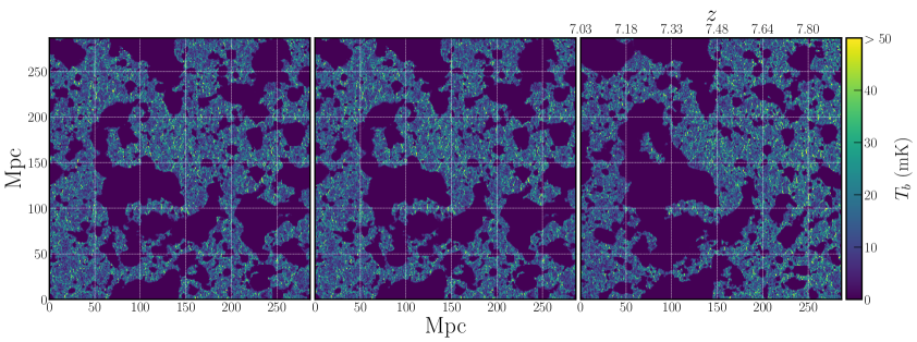
Figure 1: The brightness temperature maps $T_{b}$ for the reionization snapshot without sampling (left), reionization snapshot with sampling (middle) and light-cone simulation using $N_{\rm RS}=26$ (right). All three simulations are centred at $z=7.458$.

In the third step, we generate the reionization snapshots (RS) using a semi-numerical reionization code (see e.g. [25, 60]). This closely follows the excursion-set formalism of [67], and employs the homogeneous recombination scheme as used in [68]. Our reionization model assumes that the hydrogen follows the underlying dark matter distribution, and the ionizing sources are hosted in the dark matter halos whose masses exceed a minimum halo mass $M_{\rm min}$. Further, the number of ionizing photons emitted by a source is assumed to be directly proportional to the mass of its host halo with a proportionality constant $N_{\rm ion}$. In addition to $M_{\rm min}$ and $N_{\rm ion}$, our reionization simulations have a third free parameter, namely the mean free path of the ionizing photon $R_{\rm mfp}$ (see e.g. [25, 69] for a detailed description of the parameters). Setting different values of these parameters creates different reionization histories. For the present work, we have used the parameter values $N_{\rm ion}=23.21$, $R_{\rm mfp}=20$ Mpc and $M_{\rm min}=1.09\times 10^{9}\,{\rm M}_{\odot}$, which results in a complete reionization by $z\sim 6$ and a 50% ionization by $z\sim 8$ (see e.g. figure 1 of [25]). This reionization history is consistent with [70].

Each reionization snapshot consists of a 3D H I density field represented on a grid. Note that this grid is $8$ times coarser than that for force calculation in the $N$-body simulations. To calculate the 21-cm signal in redshift space, we represent the simulated H I density field using H I particles (see e.g. [59]) whose positions and peculiar velocities are the same as the particles in the $N$-body simulation. The neutral hydrogen fractions $x_{H~{}{\scriptsize I}}$  from eight adjacent grid points are interpolated in each particle position to calculate their H I masses. We have further randomly sampled the $N$-body particle distribution to bring down the number of H I particles by a factor of eight, which substantially cuts down the computation time and memory requirement. We have checked that this sampling affects the final power spectrum $P(k)$ only at the largest $k$ values $(k\sim 4\,{\rm Mpc}^{-1})$ where there is a $\sim 20\%$ decrement, and the change is less than $1\%$ for $k\leq 2\,{\rm Mpc}^{-1}$. The left and middle panels of Figure 1 show the 21-cm brightness temperature map for a reionization snapshot at $z=7.458$ without and with the particle sampling respectively. We notice that the two images are practically indistinguishable.

2.1 Simulating the Lightcone 21-cm Signal

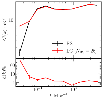
Figure 2: The top panel shows the spherically averaged 21-cm power spectrum and its 1$\sigma$ error bars for reionization snapshot and LC(26) simulation. The bottom panel shows the percentage difference ${\rm d}(k)=\left(\left|\Delta^{2}_{\rm LC}-\Delta^{2}_{\rm RS}\right|/{\Delta^{2}_{\rm RS}}\right)\times 100\%$. The error bars are estimated assuming Gaussian statistics.

Before accounting for the H I peculiar velocity, the near ($n$) and far ($f$) ends of the simulated LC EoR 21-cm signal respectively correspond to the frequencies (redshifts) $\nu_{n}=176.8$ MHz ($z_{n}=7.03$) and $\nu_{f}=159.2$ MHz ($z_{f}=7.92$). This extends from $r_{n}=8842.53$ Mpc to $r_{f}=9129.25$ Mpc (comoving) along the LoS, which exactly matches the extent of $N$-body simulation. Following [60], we have divided the radial extent $r_{f}$ to $r_{n}$ into $N_{\rm RS}$ intervals, each of comoving extent $\Delta r_{i}$. Each of these intervals corresponds to a different look back time $t_{i}$ or equivalently redshift $z_{i}$ with $i=1,2,3,...,N_{\rm RS}$. Here $N_{\rm RS}$ denotes the total number of reionization snapshots in our LC simulation, and we have a different snapshot for each $z_{i}$. Each interval $\Delta r_{i}$ is populated using H I particles drawn from a different snapshot. The comoving positions ${\bm{r}}$ of the H I particles in the entire LC simulation were used to calculate the 21-cm brightness temperature ${T_{\rm b}}(\hat{\bm{n}},\nu)$ as a function of the observed frequency $\nu$ and the LoS direction $\hat{\bm{n}}$. In addition to the cosmological expansion, the observed frequency also includes a component arising from the H I peculiar velocity. Note that the inclusion of the peculiar velocity results in some of the H I particles having frequency values beyond the boundaries of the LC box. This causes a lowering of the H I particle density near the boundaries. We calculate the frequency interval that is affected by this particle reduction, and exclude slices of this size from both the nearest and farthest sides of the LC box. After accounting for the RSD, the final LC box extends from $\nu_{f}=159.3$ MHz to $\nu_{n}=176.6$ MHz and has a central frequency of $\nu_{c}=167.94$ MHz, which corresponds to a redshift $z_{c}=7.458$; however, we do not expect this to be a large effect. Finally, we use the flat-sky approximation to map the simulated 21-cm brightness temperature distribution to a 3D $({\bm{\theta}},\nu)$ rectangular grid.

The right panel of Figure 1 shows the brightness temperature distribution for the LC simulation (using $N_{\rm RS}=26$). Comparing this with the reionization snapshots (left and middle panels), we can identify the same ionized bubbles in all the maps. However, we see that the bubble sizes are different. Considering the LC simulation, the bubble sizes evolve along the LoS direction ($x$ direction) and they are smaller at high $z$ and the sizes increase as reionization proceeds (low $z$). This clearly illustrates the fact that the EoR LC 21-cm signal is not statistically homogeneous along the LoS direction.

3 Statistical analysis

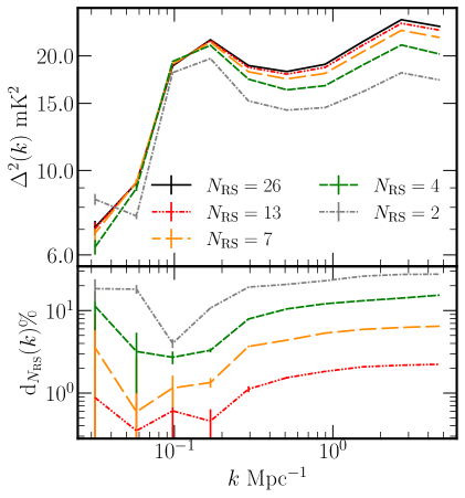
Figure 3: Top panel shows spherically averaged 21-cm 3D power spectrum for LC simulations using $N_{\rm RS}=$ 26, 13, 7, 4 and 2. The bottom panel shows the percentage difference ${\rm d}_{N_{\rm RS}}(k)$ (eq. 4.1).

3.1 The 3D power spectrum

The spherically averaged 3D power spectrum $P(k)$ can be used to quantify the two-point statistics of the LC EoR 21-cm signal. The 21-cm brightness temperature distribution ${T_{\rm b}}(\hat{\bm{n}},\nu)$ can be expressed as a function of the observing frequency $\nu$ and the angle in the plane of the sky ${\bm{\theta}}$. We map the $({\bm{\theta}},\nu)$ coordinate to $(\bm{r}_{\perp},r_{\parallel})$ which are the comoving displacements from the center of the simulation box respectively perpendicular and parallel to the LoS. Here we have used $\bm{r}_{\perp}=r_{c}{\bm{\theta}}$ and $r_{\parallel}=r^{\prime}_{c}(\nu-\nu_{c})$ where $r_{c}$ and $r^{\prime}_{c}=\frac{dr}{d\nu}|_{r_{c}}$ are both evaluated at $z_{c}$ which corresponds to $\nu_{c}$ the central frequency of the simulation. The result of this approximation is a spatially uniform rectangular grid where we can directly use 3D FFT to calculate $\tilde{T}_{b}(\bm{k})$ from ${T_{\rm b}}(\bm{r}_{\perp},r_{\parallel})$. This approximation costs less than 2% error in grid positions.

The dimensionless spherically averaged 21-cm power spectrum $\Delta^{2}(k)=k^{3}P(k)/2\pi^{2}$ is shown in Figure 2 for the LC simulation and reionization snapshot both at central redshift $z_{c}$. We see that the LC effect significantly enhances $\Delta^{2}(k)$ at large scales. The LC and RS power spectra differ by $365\%$ at the smallest $k$ bin $k=0.03$ Mpc^-1. By definition, $P(k)$ estimates the two-point statistics averaged over all three directions. It is also important to note that LC 21-cm signal ${T_{\rm b}}(\bm{\theta},\nu)$ is not statistically homogeneous (ergodic) and evolves significantly along the line-of-sight direction (Figure 1). In this case, the Fourier modes are not very optimal basis sets. The Fourier transform also imposes periodicity on the signal which cannot be justified along the LoS in the presence of the LC effect. Due to this, the power spectrum fails to quantify the entire two-point statistics of the signal and gives a biased/incomplete estimate [61, 60].

3.2 The Multi-frequency Angular Power Spectrum

In contrast to the 3D power spectrum, the Multi-frequency Angular Power Spectrum (MAPS) ${\mathcal{C}}_{\ell}(\nu_{1},\nu_{2})$ quantifies the entire second-order statistical information in the EoR 21-cm signal in the presence of LC effect (see e.g. [60, 71]). The $\bm{\theta}$ dependence of ${T_{\rm b}}(\bm{\theta},\nu)$ can be decomposed into 2D Fourier modes. The 2D Fourier transform of ${T_{\rm b}}(\bm{\theta},\nu)$ is $\tilde{T}_{\rm b}(\bm{U},\nu)$. Subsequently, the MAPS is defined as

$${\mathcal{C}}_{\ell}(\nu_{1},\nu_{2})={\mathcal{C}}_{\rm 2\pi U}(\nu_{1},\nu_{2})=\frac{1}{\Omega}\left<\tilde{T}_{\rm b}(\bm{U},\nu_{1})\tilde{T}_{\rm b}(-\bm{U},\nu_{2})\right>$$ (3.1)

where, $\bm{U}$ is the Fourier conjugate of $\bm{\theta}$ with $|\bm{U}|=\ell/2\pi$. Here, $\Omega$ is the solid angle subtended by the simulation sky at the observer point. The only assumption here is that the EoR 21-cm signal is statistically homogeneous and isotropic along different directions on the sky plane. However, no such intrinsic assumption is made along the LoS direction $\nu$.

The $\ell$ range corresponds to our LC simulations span from $\ell_{\rm min}=2\pi/\theta_{\rm max}=200$ to $\ell_{\rm max}=2\pi/\theta_{\rm min}=51215$. We divided this range into 10 equally spaced logarithmic bins. We calculated the average ${\mathcal{C}}_{\ell}(\nu_{1},\nu_{2})$ in each of these bins. For our analysis, we have chosen four $\ell$ bins, $\ell=493,1479,4484\>\text{and}\>13624$ to show our results. These $\ell$ bins correspond to large scale, two intermediate scales and small scale, respectively.

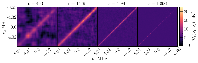
Figure 4: This shows dimensionless MAPS ${\mathcal{D}}_{\ell}(\nu_{1},\nu_{2})$ for the LC(26). MAPS for other LC($N_{\rm RS}$) with $N_{\rm RS}<26$ looks very similar, hence not shown here explicitly.

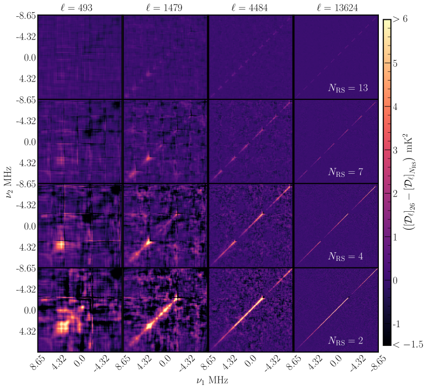
Figure 5: The difference in dimensionless MAPS ${\mathcal{D}}_{\ell}(\nu_{1},\nu_{2})$ for LC simulations using different $N_{\rm RS}<26$ with respect to LC(26) simulation: $\left[{\mathcal{D}}_{\ell}\right]_{26}-\left[{\mathcal{D}}_{\ell}\right]_{N_{\rm RS}}$.

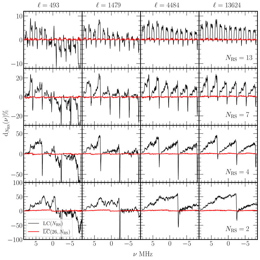
Figure 6: The percentage difference of the diagonal elements of MAPS ${\mathcal{D}}_{\ell}(\nu,\nu)$ for different LC simulations with respect to LC(26) ${\rm d}_{N_{\rm RS}}(\nu)$ (eq. 4.2). The results are shown both for before (black) and after (red) mitigation.

4 Effects of snapshot intervals

We quantify the error in the LC simulation due to the finite $N_{\rm RS}$ in terms of the spherically averaged 3D power spectrum $P(k)$ and the MAPS ${\mathcal{C}}_{\ell}(\nu_{1},\nu_{2})$. We have considered LC simulation with $N_{\rm RS}=$ 26, 13, 7, 4 and 2, and we refer to these as LC$(N_{\rm RS})$ i.e. LC(26), …, LC(2), respectively. Note that the number of cosmology snapshots ($N_{\rm CS}$) is exactly equal to the number of reionization snapshots ($N_{\rm RS}$) for all the LC simulations discussed till now, and it is not necessary to explicitly refer to $N_{\rm CS}$ in the current discussion. Further, we have used LC(26) as the reference LC simulation to compare other LC$(N_{\rm RS})$. All the LC simulations are of the same sizes and span the same $z$ range mentioned in Section 2.1.

We first discuss the results for the 3D power spectrum. The upper panel of Figure 3 shows the dimensionless 21-cm power spectrum $\Delta^{2}(k)$ for LC simulations with different values of $N_{\rm RS}$. The effects of using different $N_{\rm RS}$ are significant at both the large and the small scales. We see that for all values of $k$ the value of $\Delta^{2}(k)$ decreases as $N_{\rm RS}$ is reduced. Conversely, the power spectrum approaches its “true value” as $N_{\rm RS}$ is increased. We also notice that the values of $\Delta^{2}(k)$ appear to have converged by $N_{\rm RS}=26$ as we find only a small increment in $\Delta^{2}(k)$ as $N_{\rm RS}$ is increased from $13$ to $26$. The error bars corresponding to cosmic variance are shown in the figure. The bottom panel of Figure 3 shows the percentage difference in $\Delta^{2}(k)$ for different LC$(N_{\rm RS})$ relative to LC(26)

$${\rm d}_{N_{\rm RS}}(k)=\frac{\left|\Delta^{2}_{26}(k)-\Delta^{2}_{N_{\rm RS}}(k)\right|}{{\Delta^{2}_{26}(k)}}\times 100\%.$$ (4.1)

The overall value of ${\rm d}_{N_{\rm RS}}(k)$ at all $k$ bins increases as we decrease $N_{\rm RS}$. The value of ${\rm d}_{2}$ is $\sim 18\%$ at small $k$ bins and $\sim 27.6\%$ at the largest $k$ bin, whereas the value of ${\rm d}_{13}$ is $<1\%$ for small $k$ bins and $\sim 2.2\%$ at the largest $k$ bin. The average of ${\rm d}_{N_{\rm RS}}$ for all $k$ values are $19\%$, $9\%$, $3\%$ and $1\%$ for LC(2), LC(4), LC(7) and LC(13) respectively. Although the value of the 3D power spectrum changes with $N_{\rm RS}$, it does not provide any insight into what exactly causes this difference. This is because $P(k)$ is spherically averaged over all directions, whereas the use of different $N_{\rm RS}$ introduces discontinuities only along the LoS direction as we will explore next.

Figure 4 shows the dimensionless MAPS ${\mathcal{D}}_{\ell}(\nu_{1},\nu_{2})=\ell(\ell+1){\mathcal{C}}_{\ell}(\nu_{1},\nu_{2})/2\pi$ for the LC(26) simulation. For the convenience of plotting, we have shifted the origin of the frequency scale to $\nu_{c}$ (i.e. $\nu\rightarrow\nu-\nu_{c}$) throughout. As noted in several earlier works (e.g. [62, 72]), we see that the signal is largely localized in the vicinity of the diagonal elements $\nu_{1}=\nu_{2}$. The signal falls off rapidly away from the diagonal, and it has a very small value ${\mathcal{D}}_{\ell}(\nu_{1},\nu_{2})\approx 0$ for large frequency separations $\Delta\nu=\mid\nu_{1}-\nu_{2}\mid$. We also notice that this fall-off with increasing $\Delta\nu$ occurs faster for larger $\ell$ (e.g. [73]). For $\ell=493$ the value of ${\mathcal{D}}_{\ell}$ falls close to zero for $\Delta\nu\sim 4$ MHz, whereas this is $\Delta\nu\sim 0.25$ MHz for $\ell=13624$. The figures showing ${\mathcal{D}}_{\ell}(\nu_{1},\nu_{2})$ for smaller values of $N_{\rm RS}$ are very similar, and it is very difficult to visually distinguish these from $N_{\rm RS}=26$ and we have not explicitly shown them here. However, it is possible to visualize these differences by considering $\left([{\mathcal{D}}_{\ell}(\nu_{1},\nu_{2})]_{26}-[{\mathcal{D}}_{\ell}(\nu_{1},\nu_{2})]_{N_{\rm RS}}\right)$ shown in Figure 5. We see that the differences are visible for all the $\ell$ values, and these increase as $N_{\rm RS}$ is reduced. Further, the differences appear to follow a systematic pattern mostly close to the diagonal $\nu_{1}=\nu_{2}$, where the MAPS signal peaks. These are particularly prominent close to the “stitching boundaries” which correspond to the locations where we have joined two adjacent reionization snapshots.

To further illustrate the discontinuities due to the limited $N_{\rm RS}$, we focus on the diagonal elements of MAPS i.e. ${\mathcal{D}}_{\ell}(\nu,\nu)$. In Figure 6, we show

$${\rm d}_{N_{\rm RS}}(\nu)=\frac{\left[{\mathcal{D}}_{\ell}(\nu,\nu)\right]_{26}-\left[{\mathcal{D}}_{\ell}(\nu,\nu)\right]_{N_{\rm RS}}}{\left[{\mathcal{D}}_{\ell}(\nu,\nu)\right]_{26}}\times 100\%\,,$$ (4.2)

which quantifies the percentage difference of ${\mathcal{D}}_{\ell}(\nu,\nu)$ for LC($N_{\rm RS}$) relative to LC(26). Considering the black lines in Figure 6, as expected we find $N_{\rm RS}-1$ number of sharp discontinuities in ${\rm d}_{N_{\rm RS}}(\nu)$, one corresponding to each stitching boundary between two adjacent reionization snapshots. The peak values of ${\rm d}_{N_{\rm RS}}(\nu)$ are listed in Table 1 for the $N_{\rm RS}$ and $\ell$ values for which the results are shown in Figure 6. Considering $N_{\rm RS}=2$, we find ${\rm d}_{N_{\rm RS}}(\nu)\approx-241\%$ at the stitching boundary for the smallest $\ell$ bin. The magnitude of the discontinuity goes down, but it is still quite large ($\mid{\rm d}_{N_{\rm RS}}(\nu)\mid>50\%$) for the larger $\ell$ bins. Considering $N_{\rm RS}=4$, we see that the magnitude of the discontinuities is comparable to those for $N_{\rm RS}=2$. However, considering the mean $\mid{\rm d}_{N_{\rm RS}}(\nu)\mid$ (shown within $(...)$ in Table 1), we see that this decreases when $N_{\rm RS}$ is increased from $2$ to $4$. For example, the mean $\mid{\rm d}_{N_{\rm RS}}(\nu)\mid$ drops from $22.8\%$ to $16.1\%$ at the smallest $\ell$ bins when $N_{\rm RS}$ is increased from $2$ to $4$. Considering $N_{\rm RS}=7$ and $13$, we see that the peak ${\rm d}_{N_{\rm RS}}(\nu)$ and the mean $\mid{\rm d}_{N_{\rm RS}}(\nu)\mid$ both go down as $N_{\rm RS}$ is increased. We find a peak ${\rm d}_{N_{\rm RS}}(\nu)\approx-17\%$ and mean $\mid{\rm d}_{N_{\rm RS}}(\nu)\mid\approx 2.4\%$ at the smallest $\ell$ bin for $N_{\rm RS}=13$. The peak ${\rm d}_{N_{\rm RS}}(\nu)$ and the mean $\mid{\rm d}_{N_{\rm RS}}(\nu)\mid$ have values of $\sim 8\%$ and $\sim 2\%$ respectively at the larger $\ell$ bins for $N_{\rm RS}=13$.

We recollect that the aim here is to quantify the errors due to the finite number of reionization snapshots $N_{\rm RS}$ in the LC simulation. Ideally, we should compare the results for a finite LC($N_{\rm RS}$) with those from a continuum LC, unfortunately, the latter is not available. Here we have used LC(26) as a proxy for the continuum LC, and we use ${\rm d}_{N_{\rm RS}}(\nu)$ to quantify the error due to a limited number of $N_{\rm RS}$. We see that the error due to a finite $N_{\rm RS}$ is mainly seen as a sharp discontinuity at the stitching boundary between two adjacent reionization snapshots. The amplitude (peak ${\rm d}_{N_{\rm RS}}(\nu)$) of this discontinuity can be rather large, and it is typically found to be an order of magnitude larger than the average error which we have quantified using the mean $\mid{\rm d}_{N_{\rm RS}}(\nu)\mid$ (Table 1). It is interesting to note that the errors in the spherical power spectrum $\Delta^{2}(k)$ (Figure 3), which by definition is averaged over all directions, are comparable to the average errors in ${\mathcal{D}}_{\ell}(\nu,\nu)$. The fact that the spherical power spectrum is oblivious to the discontinuities at the stitching boundaries reiterates its limitations to fully capture the statistics of the LC simulations.

5 Mitigating the error

As discussed in Section 4, the error in the process of generating the LC 21-cm signal can be large due to the limited number $N_{\rm RS}$ of reionization snapshots. Here we propose a computationally economical method to mitigate this error by generating a large number of reionization snapshots at closely spaced time intervals. The computationally expensive cosmology snapshots, however, are only generated at large time intervals and interpolated assuming a linear cosmological evolution.

Table 1: Considering LC(26) as the reference, this lists the maximum (mean absolute) percentage difference (eq. 4.2) of ${\mathcal{D}}_{\ell}(\nu,\nu)$ for A. LC($N_{\rm RS}$) with $N_{\rm RS}=N_{\rm CS}$ ; and B. $\overline{\rm LC}(26,N_{\rm CS})$.

	$N_{\rm RS}\mid\ell$	493	1479	4484	13624
	13	-17.1 (2.39)	8.44 (1.56)	8.34 (2.23)	8.60 (2.56)
A.	7	-65.9 (6.80)	-27.1 (4.73)	23.5 (6.78)	23.8 (7.44)
	4	-268 (16.2)	-117 (10.2)	-76.2 (15.4)	46.3 (16.7)
	2	-241 (22.8)	-121 (18.1)	62.3 (26.5)	61.3 (28.8)
	13	1.12 (0.18)	0.89 (0.19)	0.80 (0.15)	0.82 (0.11)
	7	-1.65 (0.46)	-1.42 (0.33)	-1.24 (0.21)	1.43 (0.47)
B.	4	-2.87 (0.66)	-1.87 (0.52)	2.10 (0.40)	2.57 (0.81)
	2	4.74 (1.45)	4.32 (1.56)	4.51 (1.61)	3.76 (1.56)

We consider a situation where we have $N_{\rm CS}$ cosmology snapshots i.e. coeval boxes after the first two steps of the simulation process described in Section 2. As mentioned earlier, we have the dark matter particle positions, peculiar velocities and halo catalogue for each of the $N_{\rm CS}$ cosmology snapshots which correspond to redshifts $z_{i}$ with $i=1,2...,N_{\rm CS}$. Note that this is the most computationally expensive step in our simulation process, and it is advantageous to keep the value of $N_{\rm CS}$ as small as possible. The straight-forward way ahead, as discussed earlier, is to implement the third step of Section 2 and generate $N_{\rm RS}$ reionization snapshots, one for each cosmology snapshot ($N_{\rm RS}=N_{\rm CS}$). We finally stitch these together to generate LC($N_{\rm RS}$) using the methodology presented in Section 2.1. However, as already seen, we have large discontinuities (errors) in the LC simulation for small values of $N_{\rm RS}$ (Section 4).

We now present a new procedure which also starts from the same $N_{\rm CS}$ cosmology snapshots at $z_{i}$ with $i=1,2...,N_{\rm CS}$, as mentioned in the previous paragraph. However, instead of straightaway proceeding to step 3 of Section 2, we first grid the dark matter density and the halo mass density fields, and linearly interpolate these (in redshift) at $m$ redshift values between every successive pair $z_{i}$ and $z_{i+1}$. This gives us the dark matter density (also the H density) and halo mass density fields at a total of $N_{\rm CS}^{{}^{\prime}}=[N_{\rm CS}+m\times(N_{\rm CS}-1)]$ intermediate redshifts in place of the original $N_{\rm CS}$. We now implement step 3 of Section 2 to generate $N_{\rm RS}=N_{\rm CS}^{{}^{\prime}}$ reionization snapshots, which we stitch together to produce a 21-cm LC simulation. We refer to this new LC simulation as the "interpolated LC simulation" and denote this using $\overline{\rm LC}(N_{\rm RS},N_{\rm CS})$. The excursion set formalism which is used to generate the reionization snapshots, and stitching the adjacent 21-cm slices are not computationally expensive steps. It is computationally inexpensive to implement a large value of $m$ (and $N_{\rm RS}$), provided $N_{\rm CS}$ is small. Note that we also need the dark matter particle positions and peculiar velocities at the $m$ intermediate $z$ values, here we have used the values from $z_{i}$. However, we have checked that using $z_{i+1}$ also gives similar results.

We first validate the new procedure, and test how well the interpolated LC simulations $\overline{\rm LC}(N_{\rm RS},N_{\rm CS})$ match the original LC simulation LC($N_{\rm RS}$). As earlier, we consider LC(26) as the reference and compare $\overline{\rm LC}(26,13)$ against the reference. Both LC(26) and $\overline{\rm LC}(26,13)$ have been constructed from 26 reionization snapshots. However, they differ because for LC(26) every reionization snapshot also corresponds to a different cosmology snapshot, whereas we have used only $N_{\rm CS}=13$ cosmology snapshots for $\overline{\rm LC}(26,13)$ where the other 13 intermediate reionization snapshots were generated by interpolating the H and halo density fields. We have similarly also generated $\overline{\rm LC}(26,N_{\rm CS})$ for $N_{\rm CS}=2,4$ and $7$. The red lines in Figure 6 show the percentage error (eq. 4.2) in ${\mathcal{D}}_{\ell}(\nu,\nu)$ for $\overline{\rm LC}(26,N_{\rm CS})$ with respect to LC(26). We see that the errors have been considerably reduced, and these are now very close to zero. The peak error and the mean absolute error are both listed in Table 1. The improvement achieved through the interpolated simulations is quite evident for all values of $N_{\rm CS}$. The magnitude of the peak errors is $<2\%$ for $N_{\rm CS}=13,7$ while this is $<3\%$ for $N_{\rm CS}=4$. Considering the extreme case where $N_{\rm CS}=2$, we see that the magnitude of the peak error is $<5\%$ for the interpolated LC simulations as against $\sim 200\%$ for LC(2) where we do not interpolate. Note that the computational requirement for $\overline{\rm LC}(26,2)$ is approximately sixteen times smaller than that for LC$(26)$, whereas the differences are less than $5\%$ at maximum and $<2\%$ on average. It is quite evident that interpolated LC simulations are very close to the LC simulations provided we have the same number of reionization snapshots. The interpolation, however, allows us to significantly cut down the computational costs, and this provides a very economical and efficient technique to generate LC simulations.

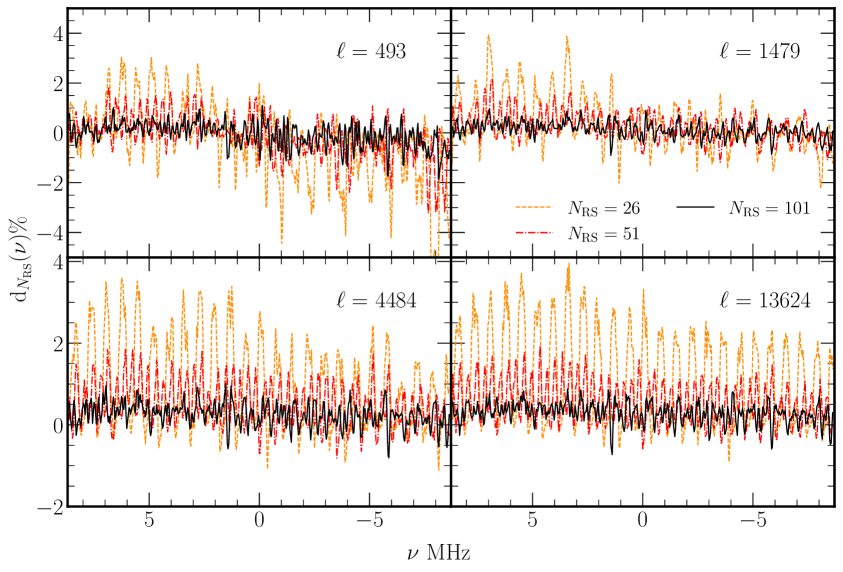
Figure 7: The percentage error in ${\mathcal{D}}_{\ell}(\nu,\nu)$ for LC simulations with $N_{\rm RS}\geq 26$. Here ${\rm d}_{N_{\rm RS}}(\nu)$ (eq. 4.2) is the percentage error of LC($N_{\rm RS}$) relative to the LC simulation with the next higher value of $N_{\rm RS}$.

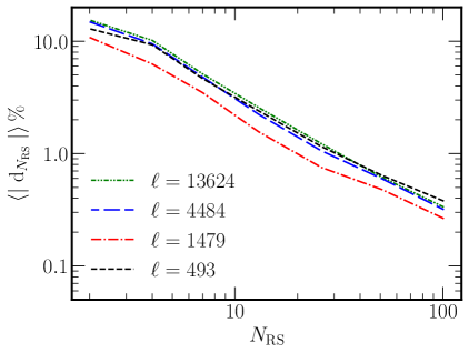
Figure 8: The mean absolute percentage error $\left<\mid{\rm d}_{N_{\rm RS}}\mid\right>$ in ${\mathcal{D}}_{\ell}(\nu,\nu)$ for LC$(N_{\rm RS})$ as a function of $N_{\rm RS}$ for different $\ell$ values.

We now use the new procedure described above to generate interpolated LC simulations using all the $N_{\rm CS}=26$ available cosmology snapshots. We have considered $m=1,3$ and $7$ which provides us with interpolated LC simulations $\overline{\rm LC}(N_{\rm RS},26)$ with $N_{\rm RS}=51,101$ and $201$ respectively. We expect these to match the corresponding LC simulations to within a few percent (possibly better than $1\%$) accuracies, and for the subsequent discussion, we drop the distinction and refer to these three interpolated LC simulations as LC(51), LC(101) and LC(201) respectively. We now effectively have LC($N_{\rm RS})$ with $N_{\rm RS}=[2,4,7,13,26,51,101,201]$, and we use ${\rm d}_{N_{\rm RS}}(\nu)$ to quantify the percentage difference in ${\mathcal{D}}_{\ell}(\nu,\nu)$ between any two LC simulations with successive $N_{\rm RS}$ values. For example, ${\rm d}_{26}(\nu)$ is the percentage difference of $N_{\rm RS}=26$ relative to $N_{\rm RS}=51$. Considering ${\rm d}_{26}(\nu)$ shown in Figure 7, we see that we still have the discontinuities at the stitching boundaries, but the amplitude has come down considerably ($<4\%$ everywhere barring one point where it is $\sim-7\%$) as compared to the much larger values seen in Figure 6. Considering even larger values of $N_{\rm RS}$, we see that the amplitude of the discontinuities drops further to $\sim 2\%$ and $1\%$ for ${\rm d}_{51}(\nu)$ and ${\rm d}_{101}(\nu)$ respectively.

We next consider $\langle\mid{\rm d}_{N_{\rm RS}}\mid\rangle$ which is the mean absolute ${\rm d}_{N_{\rm RS}}(\nu)$ (averaged over $\nu$) for a fixed $\ell$ and $N_{\rm RS}$. This provides an overall quantitative picture of the errors in the LC simulation due to the discrete number of reionization snapshots. Figure 8 shows $\langle\mid{\rm d}_{N_{\rm RS}}\mid\rangle$ as a function of $N_{\rm RS}$ for different values of $\ell$. For all values of $\ell$, we find the approximate scaling $\langle\mid{\rm d}_{N_{\rm RS}}\mid\rangle\propto N_{\rm RS}^{-1}$. Note that for the smallest $\ell$ bin, the scaling holds only if we discard the two smallest $N_{\rm RS}$ values. The average absolute percentage error in $\Delta^{2}(k)$ (Figure 9) also shows a similar $\approx N_{\rm RS}^{-1}$ scaling for the three largest $k$ bins, however, the smaller $k$ bins show a steeper scaling (in the range $-2.5$ to $-1.5$).

6 Summary and Conclusions.

During EoR, the mean neutral hydrogen fraction $\bar{x}_{\rm HI}$ evolves significantly along the LoS direction due to the LC effect. It is essential to properly incorporate this in simulations of the EoR 21-cm signal. The LC 21-cm signal is typically simulated by stitching together a finite number ($N_{\rm RS}$) of reionization snapshots, each corresponding to a different epoch. In this paper, we have quantified the errors due to the finite value of $N_{\rm RS}$. The simulations here span $286.7$ covering Mpc, which correspond to the redshift range $z=7.917$ to $7.032$ where $\bar{x}_{\rm HI}$ evolves from $0.477$ to $0.157$. We use the diagonal elements of the dimensionless MAPS ${\mathcal{D}}_{\ell}(\nu,\nu)$ to quantify the error. We find that the main effect is to introduce discontinuities in the simulated 21-cm signal at the stitching boundaries between two adjacent snapshots. Considering the extreme case with $N_{\rm RS}=2$ we find a peak error of $-241\%$ at the stitching boundary where $\bar{x}_{\rm HI}$ jumps by $0.2$. In this case, the mean absolute error is $\sim 23\%$, which is approximately an order of magnitude smaller. Considering LC$(13)$ we see that the maximum jump in $\bar{x}_{\rm HI}$ at the stitching boundaries is $0.02$, which is an order of magnitude lower compared to $N_{\rm RS}=2$. In this case, the peak error drops to $-17.1\%$ and the mean absolute error is $\sim 3\%$. We observe that the error decreases as we increase $N_{\rm RS}$ whereby abrupt changes in $\bar{x}_{\rm HI}$ at the stitching boundaries become more gradual. However, the difficulty arises in that it is computationally expensive to increase the number of snapshots that go into the 21-cm LC simulation.

Analyzing the computational costs, the major expense goes into the first two steps (Section 2) where we simulate the cosmology snapshot which jointly refers to the dark matter particle positions, peculiar velocities and halo catalogue. It is relatively inexpensive to apply the excursion set formalism (the third step in Section 2) on a cosmology snapshot to generate the reionization snapshot. Typically we use $N_{\rm CS}=N_{\rm RS}$ where $N_{\rm CS}$ is the number of cosmology snapshots i.e. we generate a separate cosmology snapshot for each reionization snapshot that we wish to simulate. The limitation for increasing the accuracy of 21-cm LC simulations comes from the computationally expensive cosmology snapshots which limit the value of $N_{\rm RS}$.

In this paper we introduce a technique to increase $N_{\rm RS}$ keeping $N_{\rm CS}$ fixed. The underlying idea is to generate $N_{\rm CS}$ cosmology snapshots at a few well separated redshifts, and then interpolate the gridded dark matter and halo fields to several ($N_{\rm RS}$) closely spaced intermediate redshifts for which we simulate reionization snapshots. The resulting interpolated LC simulation which has $N_{\rm RS}>N_{\rm CS}$ allows us to reduce both, the discontinuities at the stitching boundaries as well as the overall mean absolute error without incurring a significant increase in the computational expenses. Considering a fixed $N_{\rm RS}=26$, we demonstrate (Figure 6) that the interpolated LC simulations which have $N_{\rm CS}<N_{\rm RS}$ closely match the LC simulation which has $N_{\rm CS}=N_{\rm RS}$. In fact, considering the extreme case with $N_{\rm CS}=2$ we find that this matches the results for $N_{\rm CS}=26$ with better than $5\%$ accuracy (Table 1). This effectively validates our interpolated LC simulations which have $N_{\rm CS}<N_{\rm RS}$ as a good proxy for the computationally more expensive LC simulations which have $N_{\rm CS}=N_{\rm RS}$. Proceeding further, we fix $N_{\rm CS}=26$ for which we consider interpolated LC simulations with $N_{\rm RS}=51,101$ and $201$. Comparing the results for $N_{\rm RS}=101$ with those for $201$ (Figure 7), we see that the relative differences are less than $\sim 1\%$ which indicates a high level of convergence for the LC simulation. We expect a very small improvement ($<1\%$) if $N_{\rm RS}$ is increased any further. We have also studied how the mean absolute error $\left<\mid{\rm d}_{N_{\rm RS}}\mid\right>$ for the LC simulation changes if $N_{\rm RS}$ is varied. We find that this shows a scaling $\left<\mid{\rm d}_{N_{\rm RS}}\mid\right>\propto N_{\rm RS}^{-1}$ (Figure 8) for all the $\ell$ bins considered here. Similar behaviour is also observed at large $k$ for the 3D spherical power spectrum (Figure 9).

In conclusion, it is important to accurately incorporate the LC effect in simulations of the EoR 21-cm signal. This is particularly relevant in order to correctly interpret the signal when it is detected. Here we have quantified the errors in the 21-cm LC simulations due to the finite number of snapshots. We have shown how these errors can be controlled by increasing the number of snapshots, and we have also demonstrated a technique to achieve this within limited computational expenses. Most earlier predictions of the EoR 21-cm LC signal have used a limited number of snapshots. Further, the number of statistically independent realizations also have been limited. In future works, we plan to use the technique developed here to perform accurate 21-cm LC simulations for a variety of reionization models. We propose to use multiple realizations to analyze the statistics of the expected 21-cm signal and make predictions for ongoing and future EoR experiments.

Appendix A Errors in 3D power spectrum

Figure 9 shows $\langle\mid{\rm d}_{N_{\rm RS}}\mid\rangle$ the mean absolute percentage error in $\Delta^{2}(k)$ for 21 cm LC simulations with different $N_{\rm RS}$. We find that this scales as $\langle\mid{\rm d}_{N_{\rm RS}}\mid\rangle\propto N_{\rm RS}^{-1}$ for the three larger $k$ bins. However, the scaling is steeper with exponent $-2.31$ and $-1.84$ for the smallest and the second smallest $k$ bins respectively. Notice that this is different from the behaviour in Figure 8 where we have a $-1$ scaling for all the $\ell$ bins.

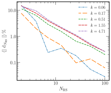
Figure 9: The mean absolute percentage error in $\Delta^{2}(k)$ versus $N_{\rm RS}$ for different $k$ bins.

References

- [1] R.H. Becker, X. Fan, R.L. White, M.A. Strauss, V.K. Narayanan, R.H. Lupton et al., Evidence for reionization at z 6: Detection of a gunn-peterson trough in az= 6.28 quasar, The Astronomical Journal 122 (2001) 2850.
- [2] G.D. Becker, J.S. Bolton, P. Madau, M. Pettini, E.V. Ryan-Weber and B.P. Venemans, Evidence of patchy hydrogen reionization from an extreme ly trough below redshift six, Monthly Notices of the Royal Astronomical Society 447 (2015) 3402.
- [3] X. Fan, V.K. Narayanan, M.A. Strauss, R.L. White, R.H. Becker, L. Pentericci et al., Evolution of the ionizing background and the epoch of reionization from the spectra of z 6 quasars, The Astronomical Journal 123 (2002) 1247.
- [4] X. Fan, M.A. Strauss, R.H. Becker, R.L. White, J.E. Gunn, G.R. Knapp et al., Constraining the evolution of the ionizing background and the epoch of reionization with z 6 quasars. ii. a sample of 19 quasars, The Astronomical Journal 132 (2006) 117.
- [5] S. Gallerani, T.R. Choudhury and A. Ferrara, Constraining the reionization history with qso absorption spectra, Monthly Notices of the Royal Astronomical Society 370 (2006) 1401.
- [6] S.E. Bosman, X. Fan, L. Jiang, S. Reed, Y. Matsuoka, G. Becker et al., New constraints on lyman- opacity with a sample of 62 quasarsat , Monthly Notices of the Royal Astronomical Society 479 (2018) 1055.
- [7] S.E. Bosman, D. , F.B. Davies and A.-C. Eilers, A comparison of quasar emission reconstruction techniques for lyman and lyman transmission, Monthly Notices of the Royal Astronomical Society 503 (2021) 2077.
- [8] A.-C. Eilers, F.B. Davies and J.F. Hennawi, The opacity of the intergalactic medium measured along quasar sightlines at , The Astrophysical Journal 864 (2018) 53.
- [9] A.-C. Eilers, J.F. Hennawi, F.B. Davies and J. Oorbe, Anomaly in the opacity of the post-reionization intergalactic medium in the ly and ly forest, The Astrophysical Journal 881 (2019) 23.
- [10] J. Yang, F. Wang, X. Fan, J.F. Hennawi, F.B. Davies, M. Yue et al., Measurements of the intergalactic medium optical depth and transmission spikes using a new quasar sample, The Astrophysical Journal 904 (2020) 26.
- [11] I.D. McGreer, A. Mesinger and V. D’Odorico, Model-independent evidence in favour of an end to reionization by , MNRAS 447 (2014) 499.
- [12] Planck Collaboration, N. Aghanim, Y. Akrami, M. Ashdown, J. Aumont, C. Baccigalupi et al., Planck 2018 results. VI. Cosmological parameters, Astronomy & Astrophysics 641 (2020) A6 [1807.06209].
- [13] S. Malhotra and J.E. Rhoads, Luminosity functions of ly emitters at redshifts and : Evidence against reionization at , The Astrophysical Journal 617 (2004) L5.
- [14] E. Hu, L. Cowie, A. Barger, P. Capak, Y. Kakazu and L. Trouille, An atlas of z= 5.7 and z= 6.5 ly emitters, The Astrophysical Journal 725 (2010) 394.
- [15] N. Kashikawa, K. Shimasaku, Y. Matsuda, E. Egami, L. Jiang, T. Nagao et al., Completing the census of ly emitters at the reionization epoch, The Astrophysical Journal 734 (2011) 119.
- [16] H. Jensen, P. Laursen, G. Mellema, I.T. Iliev, J. Sommer-Larsen and P.R. Shapiro, On the use of ly emitters as probes of reionization, Monthly Notices of the Royal Astronomical Society 428 (2013) 1366.
- [17] H. Jensen, M. Hayes, I. Iliev, P. Laursen, G. Mellema and E. Zackrisson, Studying reionization with the next generation of ly emitter surveys, Monthly Notices of the Royal Astronomical Society 444 (2014) 2114.
- [18] S. Santos, D. Sobral and J. Matthee, The ly luminosity function at z= 5.7–6.6 and the steep drop of the faint end: implications for reionization, Monthly Notices of the Royal Astronomical Society 463 (2016) 1678.
- [19] M. Ouchi, K. Shimasaku, H. Furusawa, T. Saito, M. Yoshida, M. Akiyama et al., Statistics of 207 ly emitters at a redshift near 7: Constraints on reionization and galaxy formation models, The Astrophysical Journal 723 (2010) 869.
- [20] A. Faisst, P. Capak, C.M. Carollo, C. Scarlata and N. Scoville, Spectroscopic observation of ly emitters at z 7.7 and implications on re-ionization, The Astrophysical Journal 788 (2014) 87.
- [21] A. Konno, M. Ouchi, Y. Ono, K. Shimasaku, T. Shibuya, H. Furusawa et al., Accelerated evolution of the ly luminosity function at revealed by the subaru ultra-deep survey for ly emitters at , The Astrophysical Journal 797 (2014) 16.
- [22] K. Ota, M. Iye, N. Kashikawa, A. Konno, F. Nakata, T. Totani et al., A new constraint on reionization from the evolution of the ly luminosity function at z 6–7 probed by a deep census of z= 7.0 ly emitter candidates to 0.3 l, The Astrophysical Journal 844 (2017) 85.
- [23] B.E. Robertson, S.R. Furlanetto, E. Schneider, S. Charlot, R.S. Ellis, D.P. Stark et al., New constraints on cosmic reionization from the 2012 hubble ultra deep field campaign, The Astrophysical Journal 768 (2013) 71.
- [24] B.E. Robertson, R.S. Ellis, S.R. Furlanetto and J.S. Dunlop, Cosmic reionization and early star-forming galaxies: A joint analysis of new constraints from planck and the hubble space telescope, The Astrophysical Journal Letters 802 (2015) L19.
- [25] R. Mondal, S. Bharadwaj and S. Majumdar, Statistics of the epoch of reionization (EoR) 21-cm signal - II. The evolution of the power-spectrum error-covariance, MNRAS 464 (2017) 2992 [1606.03874].
- [26] S. Mitra, T.R. Choudhury and A. Ferrara, Cosmic reionization after planck ii: contribution from quasars, Monthly Notices of the Royal Astronomical Society 473 (2017) 1416.
- [27] S. Mitra, T.R. Choudhury and B. Ratra, First study of reionization in the planck 2015 normalized closed cdm inflation model, Monthly Notices of the Royal Astronomical Society 479 (2018) 4566.
- [28] W.-M. Dai, Y.-Z. Ma, Z.-K. Guo and R.-G. Cai, Constraining the reionization history with cmb and spectroscopic observations, Physical Review D 99 (2019) 043524.
- [29] S.R. Furlanetto, S. Peng Oh and F.H. Briggs, Cosmology at low frequencies: The 21cm transition and the high-redshift universe, Physics Reports 433 (2006) 181.
- [30] J.R. Pritchard and A. Loeb, 21 cm cosmology in the 21st century, Reports on Progress in Physics 75 (2012) 086901.
- [31] J.D. Bowman, A.E. Rogers and J.N. Hewitt, Toward empirical constraints on the global redshifted 21 cm brightness temperature during the epoch of reionization, The Astrophysical Journal 676 (2008) 1.
- [32] J.D. Bowman, A.E. Rogers, R.A. Monsalve, T.J. Mozdzen and N. Mahesh, An absorption profile centred at 78 megahertz in the sky-averaged spectrum, Nature 555 (2018) 67.
- [33] S. Singh, R. Subrahmanyan, N.U. Shankar, M.S. Rao, B. Girish, A. Raghunathan et al., Saras 2: a spectral radiometer for probing cosmic dawn and the epoch of reionization through detection of the global 21-cm signal, Experimental Astronomy 45 (2018) 269.
- [34] G. Swarup, S. Ananthakrishnan, V.K. Kapahi, A.P. Rao, C.R. Subrahmanya and V.K. KulkarniCurrent Science 60 (1991) 95.
- [35] A. Ghosh, J. Prasad, S. Bharadwaj, S.S. Ali and J.N. Chengalur, Characterizing foreground for redshifted 21 cm radiation: 150 mhz giant metrewave radio telescope observations, Monthly Notices of the Royal Astronomical Society 426 (2012) 3295.
- [36] G. Paciga, J.G. Albert, K. Bandura, T.-C. Chang, Y. Gupta, C. Hirata et al., A simulation-calibrated limit on the Hi power spectrum from the GMRT Epoch of Reionization experiment, Monthly Notices of the Royal Astronomical Society 433 (2013) 639 [https://academic.oup.com/mnras/article-pdf/433/1/639/18722461/stt753.pdf].
- [37] M.P. van Haarlem, M.W. Wise, A. Gunst, G. Heald, J.P. McKean, J.W. Hessels et al., Lofar: The low-frequency array, Astronomy & astrophysics 556 (2013) A2.
- [38] S. Yatawatta, A. De Bruyn, M.A. Brentjens, P. Labropoulos, V. Pandey, S. Kazemi et al., Initial deep lofar observations of epoch of reionization windows-i. the north celestial pole, Astronomy & Astrophysics 550 (2013) A136.
- [39] A.R. Parsons, A. Liu, J.E. Aguirre, Z.S. Ali, R.F. Bradley, C.L. Carilli et al., New limits on 21 cm epoch of reionization from paper-32 consistent with an x-ray heated intergalactic medium at z= 7.7, The Astrophysical Journal 788 (2014) 106.
- [40] Z.S. Ali, A.R. Parsons, H. Zheng, J.C. Pober, A. Liu, J.E. Aguirre et al., 64 constraints on reionization: the 21 cm power spectrum at z= 8.4, The Astrophysical Journal 809 (2015) 61.
- [41] D.C. Jacobs, J.C. Pober, A.R. Parsons, J.E. Aguirre, Z.S. Ali, J. Bowman et al., Multiredshift limits on the 21 cm power spectrum from paper, The Astrophysical Journal 801 (2015) 51.
- [42] J.D. Bowman, I. Cairns, D.L. Kaplan, T. Murphy, D. Oberoi, L. Staveley-Smith et al., Science with the murchison widefield array, Publications of the Astronomical Society of Australia 30 (2013) .
- [43] S.J. Tingay, R. Goeke, J.D. Bowman, D. Emrich, S.M. Ord, D.A. Mitchell et al., The murchison widefield array: The square kilometre array precursor at low radio frequencies, Publications of the Astronomical Society of Australia 30 (2013) .
- [44] J.S. Dillon, A. Liu, C.L. Williams, J.N. Hewitt, M. Tegmark, E.H. Morgan et al., Overcoming real-world obstacles in 21 cm power spectrum estimation: A method demonstration and results from early murchison widefield array data, Physical Review D 89 (2014) 023002.
- [45] M.F. Morales, Power spectrum sensitivity and the design of epoch of reionization observatories, The Astrophysical Journal 619 (2005) 678.
- [46] M. McQuinn, O. Zahn, M. Zaldarriaga, L. Hernquist and S.R. Furlanetto, Cosmological parameter estimation using 21 cm radiation from the epoch of reionization, The Astrophysical Journal 653 (2006) 815.
- [47] S.S. Ali, S. Bharadwaj and J.N. Chengalur, Foregrounds for redshifted 21-cm studies of reionization: Giant meter wave radio telescope 153-mhz observations, Monthly Notices of the Royal Astronomical Society 385 (2008) 2166.
- [48] S. Furlanetto, A. Lidz, A. Loeb, M. McQuinn, J. Pritchard, P. Shapiro et al., Cosmology from the highly-redshifted 21 cm line, arXiv preprint arXiv:0902.3259 (2009) .
- [49] D.R. DeBoer, A.R. Parsons, J.E. Aguirre, P. Alexander, Z.S. Ali, A.P. Beardsley et al., Hydrogen epoch of reionization array (hera), Publications of the Astronomical Society of the Pacific 129 (2017) 045001.
- [50] G. Mellema, L.V. Koopmans, F.A. Abdalla, G. Bernardi, B. Ciardi, S. Daiboo et al., Reionization and the cosmic dawn with the square kilometre array, Experimental Astronomy 36 (2013) 235.
- [51] L.e.a. Koopmans, Advancing astrophysics with the square kilometre array (aaska14), .
- [52] R. Barkana and A. Loeb, Light-cone anisotropy in 21-cm fluctuations during the epoch of reionization, Monthly Notices of the Royal Astronomical Society: Letters 372 (2006) L43.
- [53] K. Zawada, B. Semelin, P. Vonlanthen, S. Baek and Y. Revaz, Light-cone anisotropy in the 21 cm signal from the epoch of reionization, Monthly Notices of the Royal Astronomical Society 439 (2014) 1615.
- [54] K.K. Datta, G. Mellema, Y. Mao, I.T. Iliev, P.R. Shapiro and K. Ahn, Light-cone effect on the reionization 21-cm power spectrum, Monthly Notices of the Royal Astronomical Society 424 (2012) 1877.
- [55] K.K. Datta, H. Jensen, S. Majumdar, G. Mellema, I.T. Iliev, Y. Mao et al., Light cone effect on the reionization 21-cm signal–ii. evolution, anisotropies and observational implications, Monthly Notices of the Royal Astronomical Society 442 (2014) 1491.
- [56] S. Bharadwaj and S.S. Ali, The cosmic microwave background radiation fluctuations from h i perturbations prior to reionization, Monthly Notices of the Royal Astronomical Society 352 (2004) 142.
- [57] Y. Mao, P.R. Shapiro, G. Mellema, I.T. Iliev, J. Koda and K. Ahn, Redshift-space distortion of the 21-cm background from the epoch of reionization–i. methodology re-examined, Monthly Notices of the Royal Astronomical Society 422 (2012) 926.
- [58] H. Jensen, K.K. Datta, G. Mellema, E. Chapman, F.B. Abdalla, I.T. Iliev et al., Probing reionization with lofar using 21-cm redshift space distortions, Monthly Notices of the Royal Astronomical Society 435 (2013) 460.
- [59] S. Majumdar, S. Bharadwaj and T.R. Choudhury, The effect of peculiar velocities on the epoch of reionization 21-cm signal, Monthly Notices of the Royal Astronomical Society 434 (2013) 1978.
- [60] R. Mondal, S. Bharadwaj and K.K. Datta, Towards simulating and quantifying the light-cone EoR 21-cm signal, MNRAS 474 (2018) 1390 [1706.09449].
- [61] C.M. Trott, Exploring the evolution of reionization using a wavelet transform and the light cone effect, Monthly Notices of the Royal Astronomical Society 461 (2016) 126.
- [62] K.K. Datta, T.R. Choudhury and S. Bharadwaj, The multifrequency angular power spectrum of the epoch of reionization 21-cm signal, Monthly Notices of the Royal Astronomical Society 378 (2007) 119.
- [63] S. Bharadwaj and P.S. Srikant, Hi fluctuations at large redshifts: Iii—simulating the signal expected at gmrt, Journal of Astrophysics and Astronomy 25 (2004) 67.
- [64] R. Mondal, S. Bharadwaj, S. Majumdar, A. Bera and A. Acharyya, The effect of non-Gaussianity on error predictions for the Epoch of Reionization (EoR) 21-cm power spectrum., MNRAS 449 (2015) L41 [1409.4420].
- [65] R. Mondal, S. Bharadwaj and S. Majumdar, Statistics of the epoch of reionization 21-cm signal - I. Power spectrum error-covariance, MNRAS 456 (2016) 1936 [1508.00896].
- [66] R.K. Sheth and G. Tormen, An excursion set model of hierarchical clustering: ellipsoidal collapse and the moving barrier, Monthly Notices of the Royal Astronomical Society 329 (2002) 61.
- [67] S.R. Furlanetto, M. Zaldarriaga and L. Hernquist, The growth of h ii regions during reionization, The Astrophysical Journal 613 (2004) 1.
- [68] T.R. Choudhury, M.G. Haehnelt and J. Regan, Inside-out or outside-in: the topology of reionization in the photon-starved regime suggested by ly forest data, Monthly Notices of the Royal Astronomical Society 394 (2009) 960.
- [69] A.K. Shaw, S. Bharadwaj and R. Mondal, The impact of non-Gaussianity on the Epoch of Reionization parameter forecast using 21-cm power-spectrum measurements, MNRAS 498 (2020) 1480 [2005.06535].
- [70] F.B. Davies, J.F. Hennawi, E. Bañados, Z. Lukić, R. Decarli, X. Fan et al., Quantitative constraints on the reionization history from the igm damping wing signature in two quasars at z> 7, The Astrophysical Journal 864 (2018) 142.
- [71] R. Mondal, G. Mellema, S.G. Murray and B. Greig, The multifrequency angular power spectrum in parameter studies of the cosmic 21-cm signal, MNRAS 514 (2022) L31 [2203.11095].
- [72] R. Mondal, S. Bharadwaj, I.T. Iliev, K.K. Datta, S. Majumdar, A.K. Shaw et al., A method to determine the evolution history of the mean neutral Hydrogen fraction, MNRAS 483 (2019) L109 [1810.06273].
- [73] R. Mondal, A.K. Shaw, I.T. Iliev, S. Bharadwaj, K.K. Datta, S. Majumdar et al., Predictions for measuring the 21-cm multifrequency angular power spectrum using SKA-Low, MNRAS 494 (2020) 4043 [1910.05196].