Tidal Forcing on the Sun and the 11-year Solar Activity Cycle

1 Introduction

The hypothesis that a possible tidal forcing on the Sun is explicitly related to the modulations of the solar-activity cycle has gained increasing attention in the solar–geophysical science community (e.g. Scafetta, 2012, 2023; Stefani et al., 2016; Stefani, Giesecke, and Weier, 2019; Stefani, Stepanov, and Weier, 2021; Courtillot, Lopes, and Le Mouël, 2021; Charbonneau, 2022; Nataf, 2022, 2023; Horstmann et al., 2023). Specifically, the works proposing physical mechanisms of the planets co-regulating the Sun’s magnetic activity via tidal forcing have in common that V-E-J configurations would provide a fundamental periodicity of $\approx 11.0$ years able to synchronize solar dynamo functioning with these planetary configurations. Particularly Stefani and co-authors (cited works) have shown that solar helicity oscillations ($\alpha$-mechanism) may be excited with a periodic forcing of 11.07 years, like the one focused here. Although the physics and origins of the solar cycle are not entirely clear, there are advanced enough models (especially for $\alpha$-$\Omega$ dynamos, i.e. a dynamo that works with helicity and large-scale differential rotation of the magnetized fluids of the Sun) that handle instabilities in the tachocline connected to external parametric forcings.

The evidence behind the usage of V-E-J configurations as a stable tidal forcing in this problem includes several estimates and concepts: a) the original calculations by Wood (1972), with an obtained period of 11.08 years; b) an idea based on “planetary resonances” (e.g. Scafetta, 2012; Stefani, Stepanov, and Weier, 2021) with a proposed period of 11.07 years; c) the empirical determinations of V-E-J quasi-alignments (Okhlopkov, 2013) with periodicities ranging from 3.2 years to a main periodicity of $\approx$ 22 years, which implies a “half spring tidal period” of $\approx$ 11 years, etc. However, classical spectral analysis applied to approximations of the tide-generating potential on the Sun did not find any periodicity related to the $\approx 11.0$ years period (Okal and Anderson, 1975; Nataf, 2022).

Venus, Earth, and Jupiter are supposed to be conspicuous or important tidal producers but this is not a sufficient condition for raising a “combined” stable periodic forcing on the Sun. Dynamical astronomy has a long tradition of considering harmonic perturbations with arguments based on combinations of planetary orbital frequencies, $n_{i}$, of the form $k_{1}n_{1}+k_{2}n_{2}+\dots$, where $k_{i}$ are integer multipliers. Are these combinations of planetary orbital frequencies always physically significant? The answer rests on the development of a forcing function that depends on physical and orbital planetary properties. For example, when analyzing the Sun’s barycentric motion using the VSOP87 theory (Bretagnon and Francou, 1988), the expansion by Kudryavtsev and Kudryavtseva (2009) or the EPM2017H ephemeris (Cionco and Pavlov, 2018), it is interesting to note that there are several periodicities around 11.07 years; for example, $2\,n_{5}-3\,n_{6}+2\,n_{7}$ of 11.042 years period; $n_{5}+\,n_{8}$, 11.065 years; $3\,n_{5}-2\,n_{6}-8\,n_{7}$, 11.136 years; $2\,n_{5}-3\,n_{6}+3\,n_{7}-2\,n_{8}$, 11.704 years; etc., but all of these arguments are driven by giant planets (sub-indexes 5 – 8 are assigned to planets from Jupiter to Neptune), they do not involve Venus or Earth. Although these orbital solutions were not obtained to describe tidal effects, such earlier results have already hinted that a term associated directly with V-E-J configurations seems to be not significant for the Sun’s dynamics.

Taking into account all the reasoning put forward in the preceding paragraphs, we conclude that the involvement of V-E-J configurations as a tidal forcing on the Sun is still uncertain. In order to help to resolve this controversy, we propose to develop the STGP in terms of harmonic series. Indeed, at present there are no standard harmonic expansions of the STGP where the terms caused by the gravitational attraction of different planets (or combinations of them) are clearly separated and identified and which allow one to precisely estimate the absolute values of tidal forces acting on elements of the Sun and the sources of these gravitational forces. Therefore, there is a real need for an accurate development of the STGP basing on advanced expansion techniques and modern planetary ephemerides, openly available to the scientific community.

2 Development of the STGP in Terms of Harmonic Series

The expression for the STGP [$V(t)$] at an arbitrary point $M$ on the Sun at an epoch $t$ is similar to that used in the developments of the tide-generating potential of Earth and other terrestrial planets (Kudryavtsev, 2004, 2007a, 2008)

$$V(t)=\sum_{j=1}^{8}\mu_{j}\sum_{n=1}^{n_{\rm{max}}}\frac{r^{n}}{r_{j}^{n+1}(t)}P_{n}\left(\cos\psi_{j}(t)\right),$$ (1)

where $r$ is the heliocentric distance of $M$; $\mu_{j}=G\,m_{j}$ is the gravitational parameter of the $j^{th}$ attracting body of mass $m_{j}$, $G$ is the gravitational constant; $r_{j}(t)$ is the heliocentric distance of planet $j$; $\psi_{j}(t)$ is an angle between $M$ and planet $j$ as seen from the Sun’s center (Figure 1); $P_{n}$ are the Legendre polynomials of degree $n$. In our formulation, we considered the effect of all eight major planets on the STGP, so that sub-index $j=1$ stands for Mercury, 2 – for Venus, 3 – for the Earth–Moon barycenter (EMB), 4 – for Mars, 5 – for Jupiter, 6 – for Saturn, 7 – for Uranus, and 8 – for Neptune. Additionally we considered the separate effects of positions and masses of the Moon and Earth on the STGP, but the difference between the total effect originated from these two bodies and that from the EMB (as a single “body”) was proven to be negligible within the accuracy of the final series. Variable $n_{{\rm{max}}}$ defines the maximum degree of the development (to be determined experimentally during the expansion procedure).

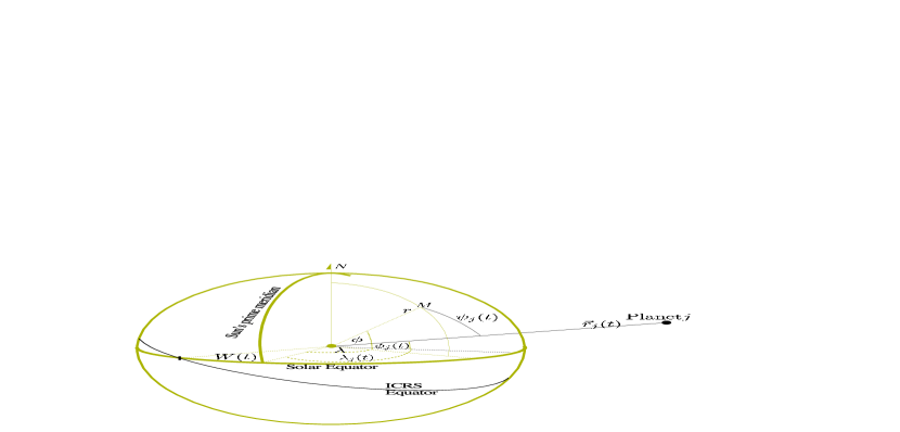
Figure 1.: Coordinate system where the STGP was developed (described in Section 2). The Sun’s North Pole is marked with $N$.

By using the Legendre addition theorem one can represent Equation 1 in the following form

$$V(t) = \sum_{n=1}^{n_{{\rm{max}}}}\left(\frac{r}{\rm{R_{\odot}}}\right)^{n}\sum_{m=0}^{n}{\bar{P}}_{nm}(\sin\phi)$$ (2)

$$\times \sum_{j=1}^{8}\Phi_{{nm}_{j}}\left(\lambda,\mu_{j},r_{j}(t),\phi_{j}(t),\lambda_{j}(t),W(t)\right),$$

where $\phi$ and $\lambda$ are the heliographic latitude and longitude of $M$, respectively; $\rm{R_{\odot}}$ is the Sun’s equatorial radius equal to 696 000 km; ${\bar{P}}_{nm}$ are the normalized associated Legendre functions of degree $n$ and order $m$ related to the non-normalized ones [$P_{nm}$] as

$${\bar{P}}_{nm}=\sqrt{\frac{\delta_{m}(2n+1)(n-m)!}{(n+m)!}}\,P_{nm};\,\delta_{m}=\left\{\begin{array}[]{l}1,\quad{\rm if}\>m=0\\ 2,\quad{\rm if}\>m\neq 0,\end{array}\right.$$ (5)

and $\Phi_{{nm}_{j}}$ is a function which includes all data related to the $j^{\rm{th}}$ attracting planet: $\mu_{j}$, $r_{j}(t)$, the heliographic latitude $\phi_{j}(t)$ and the heliographic longitude $\lambda_{j}(t)$; $W(t)$ is the Sun’s axial rotation angle reckoned along the equatorial plane of the Sun from the ascending node of this plane on the Equator of the International Celestial Reference System (ICRS) to the Sun’s prime meridian (Archinal et al., 2018). The explicit view of $\Phi_{{nm}_{j}}$-functions can be found in Kudryavtsev (2004, 2007a).

Let us denote

$$\Phi_{nm}(t)\equiv\sum_{j}^{8}\Phi_{{nm}_{j}}\left(\lambda,\mu_{j},r_{j}(t),\phi_{j}(t),\lambda_{j}(t),W(t)\right).$$ (6)

Then the task of representing the STGP by harmonic series amounts to the development of $\Phi_{nm}(t)$-functions into such series, e.g. with help of a spectral-analysis method. In order to initiate the development we first calculated and tabulated the values of $\Phi_{nm}(t)$-functions over a long time interval. As the source of planetary heliocentric coordinates we used the latest JPL’s long-term numerical ephemeris DE-441 (Park et al., 2021). The length of the development interval was about 30,000 years (the maximum time interval covered by the DE-441 ephemeris) and a sampling step of one day was chosen. We employ such a long time interval in order to have a possibility to look for and identify the expansion terms of large periods in the STGP and better separate terms of close-by frequencies. In particular, the use of a 30,000 years time interval should allow us to unambiguously separate and identify several terms with periods close to $\approx$ 11 years like those mentioned in Section 1.

At the second step, these tabulated values were processed using a modification of the spectral analysis method by Kudryavtsev (2004, 2007b). A key feature of the modified method is that it permits the development of a tabulated function to a harmonic series where both amplitudes and frequencies of the series’ terms are not constants but high-degree polynomials of time. This feature is important when the development of the STGP over a few thousand years and more is done. Over such a long time interval neither planetary motion frequencies nor amplitudes of planetary orbital perturbations can be considered as constants, but they are slowly changing variables with time (e.g. Bretagnon and Francou, 1988; Simon et al., 1994). As a consequence, the development of any function of planetary coordinates (including Equations 2 and 6) to harmonic series carries a similar temporal dependency. However, the standard Fourier transform usually indeed assumes constant frequencies and gives constant amplitudes of the expansion terms. So that application or adoption of this classical method to development of functions of planetary coordinates over thousands and tens of thousands of years can lead to significant deterioration of the expansion accuracy. As a result, over such long time intervals, the harmonic series for the STGP, where the amplitudes and arguments of each term are time polynomials, have an explicit advantage. They are essentially more compact and accurate than those that could be obtained with use of the classical Fourier transform.

Another feature of the employed method is that it directly finds the terms amplitudes at arguments which are linear combinations of mean orbital longitudes of the major planets. This allows us to explicitly identify the source of any significant peak in the STGP spectrum. More details about the development procedure as well as the accuracy of the method achieved for various planetary applications can be found in Kudryavtsev (2004, 2007b, 2016, 2017) and Cionco, Kudryavtsev, and Soon (2021).

Finally, we obtain the harmonic series for $\Phi_{nm}(t)$ of the form

$$\Phi_{nm}(t)=\sum_{i=1}^{i_{{\rm{max}}}(n,m)}\left[C_{{nm}_{i}}(t)\cos A_{{nm}_{i}}(t)+S_{{nm}_{i}}(t)\sin A_{{nm}_{i}}(t)\right],$$ (7)

with

$$C_{{nm}_{i}}(t) = {\rm C0}_{{nm}_{i}}+{\rm C1}_{{nm}_{i}}\,t+{\rm C2}_{{nm}_{i}}\,t^{2}+{\rm C3}_{{nm}_{i}}\,t^{3},$$

$$S_{{nm}_{i}}(t) = {\rm S0}_{{nm}_{i}}+{\rm S1}_{{nm}_{i}}\,t+{\rm S2}_{{nm}_{i}}\,t^{2}+{\rm S3}_{{nm}_{i}}\,t^{3},$$ (8)

${\rm C0}_{{nm}_{i}},\dots,{\rm C3}_{{nm}_{i}}$, and ${\rm S0}_{{nm}_{i}},\dots,{\rm S3}_{{nm}_{i}}$ are some derived constants; the time $t$ is reckoned in Julian centuries from the epoch J2000.0, that is, at the date of Julian day JD, $t=(\rm{JD}-2451545.0)/36525$; the arguments $A_{{nm}_{i}}(t)$ are defined as

$$A_{{nm}_{i}}(t)=m\left[W(t)+\lambda\right]+\sum_{j=1}^{8}k_{ij}l_{j}(t),$$ (9)

where $k_{ij}$ are some obtained sets of integer multipliers; $l_{j}(t)$ is a temporal polynomial expression for the mean orbital longitude of planet $j$ $(j=1,2,\dots,8)$ as given by Simon et al. (1994). In particular, the mean orbital longitudes of Jupiter and Saturn are represented by time polynomials of the sixth degree, and similar variables of other six planets are third-degree polynomials of time.

When analyzing the effect of a single planet or a linear combination of orbital longitudes of several of them on the STGP the following maximum ranges of integer multipliers $k_{ij}$ in Equation 9 were used:

• from -20 to +20 when we estimated the effect of one or a combination of two planets on the STGP;

• from -10 to +10 when the effect of three planets was evaluated.

The analysis of the final series representing our development of the STGP reveals that it is sufficient to restrict the maximum number of involved planets to three. In total we checked for about 200,000 reasonable combinations of integer multipliers $k_{ij}$. Among them the effects of around 4000 V-E-J configurations on the STGP were analyzed. Then for every argument given by Equation 9 the amplitudes $C_{{nm}_{i}}(t)$, $S_{{nm}_{i}}(t)$ in form of Equation 8 by the modified spectral analysis method (Kudryavtsev, 2004, 2007b) were determined.

Let us note that the tidal forces acting on a solar element $M(r,\,\phi,\,\lambda)$ can be straightforwardly obtained by using the same set of amplitudes $C_{{nm}_{i}}(t)$, $S_{{nm}_{i}}(t)$ and arguments $A_{{nm}_{i}}(t)$. The radial [${F}_{r}$], latitudinal [${F}_{\phi}$], and longitudinal [${F}_{\lambda}$] tidal forces (per unit of mass) at point $M$ are

$${F}_{r} = \frac{\partial V(t)}{\partial r},$$

$${F}_{\phi} = \frac{1}{r}\,\frac{\partial V(t)}{\partial\phi},$$

$${F}_{\lambda} = \frac{1}{r\cos\phi}\,\frac{\partial V(t)}{\partial\lambda},$$ (10)

where distance $r$ is positive in the direction from the Sun’s center; latitude $\phi$ is reckoned from the solar equatorial plane being positive to the North; and longitude $\lambda$ is counted from the solar prime meridian to the East (Figure 1). By substituting Equation 2 and Equation 7 to the Equations 10, one obtains

$${F}_{r} = \frac{1}{r}\sum_{n=1}^{n_{{\rm{max}}}}n\,\left(\frac{r}{\rm{R_{\odot}}}\right)^{n}\sum_{m=0}^{n}{\bar{P}}_{nm}(\sin\phi)$$

$$\times \sum_{i=1}^{i_{{\rm{max}}}(n,m)}\left[C_{{nm}_{i}}(t)\cos A_{{nm}_{i}}(t)+S_{{nm}_{i}}(t)\sin A_{{nm}_{i}}(t)\right],$$

$${F}_{\phi} = \frac{1}{r}\sum_{n=1}^{n_{{\rm{max}}}}\left(\frac{r}{\rm{R_{\odot}}}\right)^{n}\sum_{m=0}^{n}\frac{{\partial\bar{P}}_{nm}(\sin\phi)}{\partial\phi}$$

$$\times \sum_{i=1}^{i_{{\rm{max}}}(n,m)}\left[C_{{nm}_{i}}(t)\cos A_{{nm}_{i}}(t)+S_{{nm}_{i}}(t)\sin A_{{nm}_{i}}(t)\right],$$

$${F}_{\lambda} = \frac{1}{r\cos\phi}\sum_{n=1}^{n_{{\rm{max}}}}\left(\frac{r}{\rm{R_{\odot}}}\right)^{n}\sum_{m=0}^{n}m\,{\bar{P}}_{nm}(\sin\phi)$$ (11)

$$\times \sum_{i=1}^{i_{{\rm{max}}}(n,m)}\left[-C_{{nm}_{i}}(t)\sin A_{{nm}_{i}}(t)+S_{{nm}_{i}}(t)\cos A_{{nm}_{i}}(t)\right].$$

The derivatives of the associated Legendre functions can be easily evaluated using recursive formulas (e.g. Abramowitz and Stegun, 1970).

3 Results and Discussion

An accurate development of the STGP in terms of harmonic series in the form given by Equations 2 – 9 is presented, and a corresponding tidal catalog is released at sai.msu.ru/neb/ksm/tgp_sun/STGP.zip. The calculations show that the magnitude of the STGP given by Equations 1 and 2 can reach values on the order of $10^{-1}\,{\rm m}^{2}{\rm s}^{-2}$. As a consequence, the truncation threshold for the amplitudes of the terms to be included in the final STGP series was chosen to be as small as $1\times 10^{-7}{\rm m}^{2}{\rm s}^{-2}$. Then, all tidal signal above that limit is considered significant and also identifiable, that is, attributable to a specific linear combination of planetary orbital frequencies. The maximum degree of the development $n_{{\rm{max}}}$ that leads to terms of such minimum amplitudes was found to be equal to 4. Table 1 presents the number of terms obtained for every value of degree $n$ and order $m$ of the development. In total, the STGP catalog includes 713 harmonic terms.

Table 1.: Number of terms in the STGP development of degree $n$ and order $m$.

$n$	$m$
	0	1	2	3	4
2	104	155	304
3	17	30	31	36
4	4	7	8	7	10

In order to make sure that no significant term of the STGP development is missed we made the following tests. For every degree $n$ and order $m$ we calculated the “residuals function” defined as the differences between the original tabulated values of $\Phi_{nm}(t)$-functions and the representation of these values by the obtained STGP series in form of Equation 7. Then we defined a large set of frequencies corresponding to periods ranging from 0 to, e.g., several thousand years (the upper limit was a free parameter) with a small period step of $1\times 10^{-4}$ year. Finally, we made the Fourier transform of the “residuals function” at every frequency from that set and found the amplitude of the corresponding term. If the term amplitude exceeded the chosen truncation threshold we tried to identify a combination of the planetary orbital frequencies that has the same or very close period and add it to our development of the STGP. In this way we could eventually make sure that all significant terms are captured by our STGP series.

Table 2 gives the number of terms in the STGP development which include the orbital longitudes of the various number of planets in the terms arguments. When the number of involved planets is zero it means that the corresponding term is purely associated with the solar rotation or it is a constant.

Table 2.: The number of planets used in calculation of arguments of the STGP terms.

Number of planets	Number of terms
0	8
1	307
2	313
3	85

Table 3 shows how many times the orbital longitude of every planet is used in the calculation of arguments of the STGP terms.

Table 3.: Usage of orbital longitudes of planets in arguments of the STGP terms.

Planet	Number of times
Mercury	157
Venus	115
EMB	100
Mars	45
Jupiter	334
Saturn	283
Uranus	134
Neptune	20

A selection of the STGP’s terms and associated quantities is presented in Table 4. The amplitude [$Q$] and period [$T$] of every term are calculated at the J2000.0 epoch:

$$Q=\sqrt{{\rm C0^{2}}_{{nm}_{i}}+{\rm S0^{2}}_{{nm}_{i}}},$$ (12)

$$T=\frac{2\,\pi}{\dot{A}_{{nm}_{i}}(t)}$$ (13)

where $\dot{A}_{{nm}_{i}}(t)=m\,\dot{W}(t)+\sum_{j=1}^{8}k_{ij}\dot{l}_{j}(t)$. The values of $T$- and $Q$-parameters at another epoch can be obtained from the complete polynomial expressions for $C_{{nm}_{i}}$-,$S_{{nm}_{i}}$-coefficients and the terms arguments available in the on-line version of the STGP catalog (STGP.zip file). The exact calculation procedure and all necessary polynomial expressions for the terms arguments and other involved variables are given in the ReadMe file included in the STGP.zip archive. When all integer multipliers $k_{ij}$ are equal to zero, it means that the corresponding term is either a constant or its period $T$ is due to the Sun’s rotation only (e.g. terms with ranks 282 and 613). Table 4 includes all the terms with a period between 10 years and 12 years which we identify as the 11-year spectral band; in addition, the most important terms (i.e. with the largest $Q$-values) involving Venus, Earth, or Jupiter are reported. The terms are given in the decreasing order of their periods.

Table 4.: Selected terms of the STGP harmonic development ranked by decreasing period. Amplitudes [$Q$] and periods [$T$] are given at the epoch J2000.0. Periods are given in years or days (if marked by an asterisk as a superscript).

Rank	$n$	$m$	Planets Involved	$T$ [yr, d*]	$Q$ [$\times 10^{-10}$ m2s-2]
4	2	0	$l_{5}-7l_{7}$	1010.1953	$0.1516\times 10^{5}$
5	2	0	$-2l_{5}+5l_{6}$	883.2639	$0.2465\times 10^{5}$
6	2	0	$l_{8}$	164.7701	$0.2123\times 10^{4}$
7	2	0	$-l_{3}+12l_{5}$	85.8175	$0.1420\times 10^{4}$
10	2	0	$l_{5}-2l_{6}$	60.9469	$0.6607\times 10^{5}$
19	2	0	$2l_{6}-2l_{7}$	22.6801	$0.1523\times 10^{4}$
20	2	0	$l_{5}-l_{6}$	19.8589	$0.1446\times 10^{6}$
21	2	0	$-l_{5}+4l_{6}$	19.4222	$0.1861\times 10^{4}$
27	2	0	$2l_{5}-5l_{6}+7l_{7}$	12.1683	$0.6876\times 10^{4}$
28	2	0	$3l_{5}-5l_{6}$	12.0235	$0.2836\times 10^{6}$
29	2	0	$7l_{7}$	12.0029	$0.3874\times 10^{5}$
30	2	0	$l_{1}-4l_{3}-2l_{6}$	11.8774	$0.4073\times 10^{4}$
31	2	0	$l_{5}$	11.8620	$0.4179\times 10^{8}$
32	3	0	$l_{5}$	11.8620	$0.6946\times 10^{5}$
33	2	0	$3l_{5}-6l_{6}+3l_{7}$	11.7746	$0.1448\times 10^{4}$
34	2	0	$2l_{5}-7l_{7}$	11.7243	$0.3271\times 10^{5}$
35	2	0	$-l_{5}+5l_{6}$	11.7048	$0.9212\times 10^{5}$
36	2	0	$4l_{5}-7l_{6}$	10.0423	$0.6635\times 10^{4}$
37	2	0	$2l_{5}-2l_{6}$	9.9294	$0.4675\times 10^{6}$
40	2	0	$-l_{2}+2l_{3}-8l_{6}$	9.7192	$0.1013\times 10^{4}$
49	2	0	$l_{1}-4l_{3}$	6.5751	$0.8065\times 10^{5}$
76	2	0	$l_{2}-l_{3}$	1.5987	$0.2203\times 10^{4}$
80	2	0	$l_{3}$	1.0000	$0.6374\times 10^{7}$
83	2	0	$2l_{2}-2l_{3}$	291.9607*	$0.2469\times 10^{5}$
84	2	0	$4l_{2}-5l_{3}$	243.1650*	$0.3184\times 10^{4}$
85	2	0	$l_{2}-l_{5}$	236.9919*	$0.5996\times 10^{4}$
87	2	0	$l_{2}$	224.7008*	$0.5607\times 10^{7}$
92	2	0	$3l_{2}-3l_{3}$	194.6405*	$0.1491\times 10^{5}$
107	2	0	$2l_{2}-2l_{5}$	118.4960*	$0.2507\times 10^{4}$
282	2	1	$0$	25.3800*	$0.1210\times 10^{9}$
300	2	1	$l_{5}$	25.2322*	$0.3882\times 10^{7}$
359	2	2	$-2l_{1}$	17.8358*	$0.1903\times 10^{9}$
406	2	2	$-2l_{2}$	14.3059*	$0.4799\times 10^{9}$
430	2	2	$-2l_{3}$	13.6376*	$0.2242\times 10^{9}$
544	2	2	$-2l_{5}$	12.7648*	$0.4967\times 10^{9}$
555	2	2	$l_{2}-2l_{3}+7l_{6}$	12.7506*	$0.1862\times 10^{5}$
613	2	2	$0$	12.6900*	$0.5515\times 10^{7}$

Although the obtained tidal periods range from $\approx$ 1000 years to 1 week, we do not find any $\approx$ 11.0 years period. The V-E-J configurations do not produce any significant tidal term at this or other periods. No term with an $\approx 22.0$ years period is found either. The 11-year spectral band is dominated by Jupiter’s orbital motion (terms with rank 31 and 32), followed by a combined term originated from both Jupiter and Saturn motions (rank 35). No term due to Venus is found in the 11-year spectral band: the term arisen from the argument $-l_{2}+2l_{3}-8l_{6}$ (rank 40) with a period of 9.7192 years is the closest one. The planet that contributes the most to the STGP in three-planets configurations, along with Venus and Earth, is Saturn (e.g. rank 40, 555). Mercury is involved in several periods larger than 1 year (i.e. larger than its orbital period), and especially in the 11-year spectral band (rank 30).

In general, the more planets constitute the argument of an STGP term, the less should be the term’s amplitude and its effect on solar tides. To show this, let us note that the main form of the tide-generating potential on the planet’s (or Sun’s) surface coincides with the form of the disturbing function acting on a planet’s satellite from other attracting planets (see, e.g., Musen, Bailie, and Upton, 1961; Kaula, 1962), if we assume the height of the satellite above the planetary surface is equal (just formally) to zero. Analytic representation of the satellite motion reveals arguments which can simultaneously include orbital frequencies of two or three (or more) planets. It happens when we calculate the satellite orbital perturbations of the second or third (or higher) order, respectively. However, it is well known that amplitudes of higher-order terms are in general much less than those of lower-order terms (if there are no resonant arguments). Then, it is expected that an STGP term with an argument including orbital frequencies of three planets (such us Venus, Earth, and Jupiter) should also have an essentially weaker effect on the STGP and solar tides than terms of about the same frequency but originating from motions of one or two planets.

4 Conclusions

Various V-E-J configurations do not produce any significant term in the STGP harmonic development. An $\approx 11.0$ years tidal period with a direct physical relevance to the 11-year-like solar-activity cycle is highly improbable. We can conclude that a combined effect of three (and more) planets should have a much weaker effect on the STGP than the effect of one or two planets.

The solar barycentric movement was already studied by using current methods of celestial mechanics, both analytically (Bretagnon and Francou, 1988) and numerically (Kudryavtsev and Kudryavtseva, 2009; Cionco and Pavlov, 2018). Now we complete the study of solar barycentric dynamics with the standard development of the STGP in terms of harmonic series, offering a general solution for calculating the tidal forcing on the Sun. We present this research tool to the scientific community interested in these topics and propose an a priori evaluation of the tidal effect of the major planets on the Sun to avoid confusions about the relevance of various periodic terms or even spurious forcings.

Funding

This research received no specific grant from any funding agency.

Data Availability

The full output (713 terms) of the STGP catalog is available at
sai.msu.ru/neb/ksm/tgp_sun/STGP.zip

Declarations

Conflict of interest

The authors declare that they have no conflicts of interest.

References

- Abramowitz and Stegun (1970) Abramowitz, M., Stegun, I.A.: 1970, Handbook of Mathematical Functions: with Formulas, Graphs, and Mathematical Tables, National Bureau of Standards. ISBN 0486612724; 9780486612720.
- Archinal et al. (2018) Archinal, B.A., Acton, C.H., A’Hearn, M.F., Conrad, A., Consolmagno, G.J., Duxbury, T., Hestroffer, D., Hilton, J.L., Kirk, R.L., Klioner, S.A., McCarthy, D., Meech, K., Oberst, J., Ping, J., Seidelmann, P.K., Tholen, D.J., Thomas, P.C., Williams, I.P.: 2018, Report of the IAU Working Group on Cartographic Coordinates and Rotational Elements: 2015. Celest. Mech. Dyn. Astron. 130, 22. DOI.
- Bretagnon and Francou (1988) Bretagnon, P., Francou, G.: 1988, Planetary theories in rectangular and spherical variables-VSOP 87 solutions. A&A 202, 309.
- Charbonneau (2022) Charbonneau, P.: 2022, External Forcing of the Solar Dynamo. Front. Astron. Space Sci. 9, 853676. DOI.
- Cionco and Pavlov (2018) Cionco, R.G., Pavlov, D.A.: 2018, Solar barycentric dynamics from a new solar-planetary ephemeris. A&A 615, A153. DOI.
- Cionco, Kudryavtsev, and Soon (2021) Cionco, R.G., Kudryavtsev, S.M., Soon, W.W.-H.: 2021, Possible Origin of Some Periodicities Detected in Solar-Terrestrial Studies: Earth’s Orbital Movements. Earth Space Sci. 8, e2021EA001805. DOI.
- Courtillot, Lopes, and Le Mouël (2021) Courtillot, V., Lopes, F., Le Mouël, J.: 2021, On the Prediction of Solar Cycles. Sol. Phys. 296, 1. DOI.
- Horstmann et al. (2023) Horstmann, G.M., Mamatsashvili, G., Giesecke, A., Zaqarashvili, T.V., Stefani, F.: 2023, Tidally Forced Planetary Waves in the Tachocline of Solar-like Stars. Astrophys. J. 944, 48. DOI.
- Kaula (1962) Kaula, W.M.: 1962, Development of the lunar and solar disturbing functions for a close satellite. AJ 67, 300. DOI. ADS.
- Kudryavtsev (2004) Kudryavtsev, S.M.: 2004, Improved harmonic development of the Earth tide-generating potential. J. Geodesy 77, 829. DOI.
- Kudryavtsev (2007a) Kudryavtsev, S.M.: 2007a, Applications of the KSM03 harmonic development of the tidal potential. In: Tregoning, P., Rizos, C. (eds.) Dynamic Planet. Internat. Assoc. Geodesy Symp. 130, Springer, 511. DOI.
- Kudryavtsev (2007b) Kudryavtsev, S.M.: 2007b, Long-term harmonic development of lunar ephemeris. A&A 471, 1069. DOI.
- Kudryavtsev (2008) Kudryavtsev, S.M.: 2008, Harmonic development of tide-generating potential of terrestrial planets. Celest. Mech. Dyn. Astron. 101, 337. DOI.
- Kudryavtsev (2016) Kudryavtsev, S.M.: 2016, Analytical series representing DE431 ephemerides of terrestrial planets. MNRAS 456, 4015. DOI.
- Kudryavtsev (2017) Kudryavtsev, S.M.: 2017, Analytical series representing the DE431 ephemerides of the outer planets. MNRAS 466, 2675. DOI.
- Kudryavtsev and Kudryavtseva (2009) Kudryavtsev, S.M., Kudryavtseva, N.S.: 2009, Accurate analytical representation of Pluto modern ephemeris. Celest. Mech. Dyn. Astron. 105, 353. DOI. ADS.
- Musen, Bailie, and Upton (1961) Musen, P., Bailie, A., Upton, E.: 1961, Development of the lunar and solar perturbations in the motion of an artificial satellite. Technical Report D-494, NASA, Washington, DC.
- Nataf (2022) Nataf, H.-C.: 2022, Tidally Synchronized Solar Dynamo: A Rebuttal. Sol. Phys. 297, 107. DOI. ADS.
- Nataf (2023) Nataf, H.-C.: 2023, Response to Comment on “Tidally Synchronized Solar Dynamo: A Rebuttal”. Sol. Phys. 298, 33. DOI.
- Okal and Anderson (1975) Okal, E., Anderson, D.L.: 1975, On the planetary theory of sunspots. Nature 253, 511. DOI. ADS.
- Okhlopkov (2013) Okhlopkov, V.P.: 2013, Cycles of solar activity and the configurations of the planets. J. Phys.: CS-409, 012199. DOI.
- Park et al. (2021) Park, R.S., Folkner, W.M., Williams, J.G., Boggs, D.H.: 2021, The JPL Planetary and Lunar Ephemerides DE440 and DE441. AJ 161, 105. DOI.
- Scafetta (2012) Scafetta, N.: 2012, Does the Sun work as a nuclear fusion amplifier of planetary tidal forcing A proposal for a physical mechanism based on the mass-luminosity relation. J. Atmos. Solar-Terr. Phys. 81-82, 27. DOI.
- Scafetta (2023) Scafetta, N.: 2023, Comment on “Tidally Synchronized Solar Dynamo: A Rebuttal”. Sol. Phys. 298, 24. DOI.
- Simon et al. (1994) Simon, J.-L., Bretagnon, P., Chapront, J., Chapront-Touze, M., Francou, G., Laskar, J.: 1994, Numerical expressions for precession formulae and mean elements for the Moon and the planets. A&A 282, 663.
- Stefani, Giesecke, and Weier (2019) Stefani, F., Giesecke, A., Weier, T.: 2019, A model of a tidally synchronized solar dynamo. Sol. Phys. 294, 60. DOI.
- Stefani, Stepanov, and Weier (2021) Stefani, F., Stepanov, R., Weier, T.: 2021, Shaken and stirred: when Bond meets Suess–de Vries and Gnevyshev–Ohl. Sol. Phys. 296, 1. DOI.
- Stefani et al. (2016) Stefani, F., Giesecke, A., Weber, N., Weier, T.: 2016, Synchronized helicity oscillations: a link between planetary tides and the solar cycle? Sol. Phys. 291, 2197. DOI.
- Wood (1972) Wood, K.D.: 1972, Physical sciences: sunspots and planets. Nature 240, 91. DOI.