Abstract

In this work, we tentatively assign the $Y(4500)$ as the $[uc]_{\tilde{A}}[\overline{uc}]_{V}+[uc]_{V}[\overline{uc}]_{\tilde{A}}+[dc]_{\tilde{A}}[\overline{dc}]_{V}+[dc]_{V}[\overline{dc}]_{\tilde{A}}$ tetraquark state with the quantum numbers $J^{PC}=1^{--}$, and study the three-body strong decay $Y(4500)\to D^{*-}D^{*0}\pi^{+}$ with the light-cone QCD sum rules. It is the first time to use the light-cone QCD sum rules to calculate the four-hadron coupling constants, the approach can be extended to study other three-body strong decays directly and diagnose the $X$, $Y$ and $Z$ states.

PACS number: 12.39.Mk, 12.38.Lg

Key words: Tetraquark state, QCD sum rules

1 Introduction

In last two decays, several vector charmonium-like states have been observed, they cannot be accommodated comfortably in the traditional charmonia, we have to introduce additional quark or gluon degrees of freedom in assignments [1]. For example, the $Y(4260)$ observed in the $J/\psi\pi^{+}\pi^{-}$ invariant mass spectrum by the BaBar collaboration [2], the $Y(4220)$ and $Y(4390)$ ($Y(4320)$) observed in the $h_{c}\pi^{+}\pi^{-}$ ($J/\psi\pi^{+}\pi^{-}$) invariant mass spectrum by the BESIII collaboration [3, 4], and the $Y(4360)$ and $Y(4660)$ ($Y(4630)$) observed in the $\psi^{\prime}\pi^{+}\pi^{-}$ ($\Lambda_{c}^{+}\bar{\Lambda}_{c}^{-}$) invariant mass spectrum by the Belle collaboration [5, 6, 7] are excellent candidates for the vector tetraquark states.

In 2022, the BESIII collaboration explored the $e^{+}e^{-}\to K^{+}K^{-}J/\psi$ cross sections at center-of-mass energies from 4.127 to 4.600 GeV based on $15.6\,\rm{fb}^{-1}$ data, and observed two resonant structures, one is consistent with the established $Y(4230)$; the other was observed for the first time with a significance larger than $8\sigma$ and denoted as $Y(4500)$, its Breit-Wigner mass and width are $4484.7\pm 13.3\pm 24.1\,\rm{MeV}$ and $111.1\pm 30.1\pm 15.2\,\rm{MeV}$, respectively [8].

Recently, the BESIII collaboration explored the Born cross sections of the process $e^{+}e^{-}\to D^{*-}D^{*0}\pi^{+}$ at center-of-mass energies from 4.189 to 4.951 GeV using the data samples corresponding to an integrated luminosity of $17.9\,\rm{fb}^{-1}$ and observed three enhancements, whose masses are $4209.6\pm 4.7\pm 5.9\,\rm{MeV}$, $4469.1\pm 26.2\pm 3.6\,\rm{MeV}$ and $4675.3\pm 29.5\pm 3.5\,\rm{MeV}$, respectively, and widths are $81.6\pm 17.8\pm 9.0\,\rm{MeV}$, $246.3\pm 36.7\pm 9.4\,\rm{MeV}$ and $218.3\pm 72.9\pm 9.3\,\rm{MeV}$, respectively. The first and third resonances are consistent with the $Y(4230)$ and $Y(4660)$ states, respectively, while the second resonance is compatible with the $Y(4500)$ [9].

In fact, analogous decays were already observed in the process $e^{+}e^{-}\to Y\to\pi^{+}D^{0}D^{*-}$ for the center-of-mass energies from 4.05 to 4.60 GeV by the BESIII collaboration in 2018, and the two enhancements $Y$ lie around 4.23 and 4.40 GeV, respectively [10].

In the scenario of tetraquark states, the calculations based on the QCD sum rules have given several reasonable assignments of the $Y$ states [11, 12, 13, 14, 15, 16, 17, 18, 19, 20, 21, 22]. For example, in Ref.[22], we take the scalar, pseudoscalar, axialvector, vector and tensor (anti)diquarks to construct vector and tensor four-quark currents without introducing explicit P-waves, and explore the mass spectrum of the vector hidden-charm tetraquark states via the QCD sum rules in a comprehensive way. At the energy about $4.5\,\rm{GeV}$, we obtain three hidden-charm tetraquark states with the $J^{PC}=1^{--}$, the tetraquark states with the symbolic structures $[uc]_{\tilde{V}}[\overline{dc}]_{A}-[uc]_{A}[\overline{dc}]_{\tilde{V}}$, $[uc]_{\tilde{A}}[\overline{dc}]_{V}+[uc]_{V}[\overline{dc}]_{\tilde{A}}$ and $[uc]_{S}[\overline{dc}]_{\tilde{V}}-[uc]_{\tilde{V}}[\overline{dc}]_{S}$ have the masses $4.53\pm 0.07\,\rm{GeV}$, $4.48\pm 0.08\,\rm{GeV}$ and $4.50\pm 0.09\,\rm{GeV}$, respectively [22]. Thus we have three candidates for the $Y(4500)$, the best assignment of the symbolic structure is $[uc]_{\tilde{A}}[\overline{dc}]_{V}+[uc]_{V}[\overline{dc}]_{\tilde{A}}=Y(4500)$ comparing with the BESIII experimental data $M_{Y(4500)}=4469.1\pm 26.2\pm 3.6\,\rm{MeV}$ [9], where we have taken the isospin limit, the tetraquark states with the valence quark structures,

$$\bar{c}c\bar{d}u,\,\,\bar{c}c\bar{u}d,\,\,\bar{c}c\frac{\bar{u}u-\bar{d}d}{\sqrt{2}},\,\,\bar{c}c\frac{\bar{u}u+\bar{d}d}{\sqrt{2}}\,,$$ (1)

have degenerated masses and pole residues. As there exist three four-quark currents with the $J^{PC}=1^{--}$, which couple potentially to the vector hidden-charm tetraquark states with almost degenerated masses [22], we can also tentatively say that there only exists one vector tetraquark state with three different Fock components $[uc]_{\tilde{V}}[\overline{dc}]_{A}-[uc]_{A}[\overline{dc}]_{\tilde{V}}$, $[uc]_{\tilde{A}}[\overline{dc}]_{V}+[uc]_{V}[\overline{dc}]_{\tilde{A}}$ and $[uc]_{S}[\overline{dc}]_{\tilde{V}}-[uc]_{\tilde{V}}[\overline{dc}]_{S}$, we can choose either Fock component (in other words, current) to explore the hadronic properties. At the first step, we choose the optimal current corresponding to the optimal Fock component $[uc]_{\tilde{A}}[\overline{dc}]_{V}+[uc]_{V}[\overline{dc}]_{\tilde{A}}$, i.e. the current $J_{\mu}^{Y}(0)$ in Eq.(2) in the isospin limit. However, we cannot assign a hadron unambiguously with the mass alone, we have to explore the decay width to make more robust assignment. If we want to investigate the three-body strong decays $Y\to J/\psi\pi^{+}\pi^{-}$, $\psi^{\prime}\pi^{+}\pi^{-}$, $J/\psi K^{+}K^{-}$, $h_{c}\pi^{+}\pi^{-}$, $D^{0}D^{*-}\pi^{+}$ and $D^{*-}D^{*0}\pi^{+}$ with the QCD sum rules directly, we have to introduce four-point correlation functions, the hadronic spectral densities are complex enough to destroy the reliability of the calculations.

In this work, we tentatively assign the $Y(4500)$ as the $[uc]_{\tilde{A}}[\overline{uc}]_{V}+[uc]_{V}[\overline{uc}]_{\tilde{A}}+[dc]_{\tilde{A}}[\overline{dc}]_{V}+[dc]_{V}[\overline{dc}]_{\tilde{A}}$ tetraquark state with the $J^{PC}=1^{--}$, and extend our previous works to study the three-body strong decay $Y(4500)\to D^{*-}D^{*0}\pi^{+}$ with the light-cone QCD sum rules, where only three-point correlation function is needed. It is the first time to investigate the three-body strong decays with the light-cone QCD sum rules. In our previous works, we have obtained rigorous quark-hadron duality for the three-point correlation functions, which work very well. There are other procedures in dealing with the three-point QCD sum rules exploring the hadronic coupling constants [30, 31, 32], for detailed discussions about the differences, one can consult Refs.[23, 24].

The article is arranged as follows: we derive the light-cone QCD sum rules for the $YD^{*}\bar{D}^{*}\pi$ coupling constants in section 2; in section 3, we present numerical results and discussions; section 4 is reserved for our conclusion.

2 Light-cone QCD sum rules for the $YD^{*}\bar{D}^{*}\pi$ coupling constants

Firstly, we write down the three-point correlation function $\Pi_{\mu\alpha\beta}(p)$ in the light-cone QCD sum rules,

$$\Pi_{\mu\alpha\beta}(p,q) = i^{2}\int d^{4}xd^{4}y\,e^{-ip\cdot x}e^{-iq\cdot y}\,\langle 0|T\left\{J_{\mu}^{Y}(0)J_{\alpha}^{D^{*+}}(x)J^{\bar{D}^{*0}}_{\beta}(y)\right\}|\pi(r)\rangle\,,$$ (2)

where the currents

$$J_{\mu}^{Y}(0) = \frac{\varepsilon^{ijk}\varepsilon^{imn}}{2}\Big{[}u^{T}_{j}(0)C\sigma_{\mu\nu}\gamma_{5}c_{k}(0)\bar{u}_{m}(0)\gamma_{5}\gamma^{\nu}C\bar{c}^{T}_{n}(0)+u^{T}_{j}(0)C\gamma^{\nu}\gamma_{5}c_{k}(0)\bar{u}_{m}(0)\gamma_{5}\sigma_{\mu\nu}C\bar{c}^{T}_{n}(0)$$

$$+d^{T}_{j}(x)C\sigma_{\mu\nu}\gamma_{5}c_{k}(0)\bar{d}_{m}(0)\gamma_{5}\gamma^{\nu}C\bar{c}^{T}_{n}(0)+d^{T}_{j}(0)C\gamma^{\nu}\gamma_{5}c_{k}(0)\bar{d}_{m}(0)\gamma_{5}\sigma_{\mu\nu}C\bar{c}^{T}_{n}(0)\Big{]}\,,$$

$$J_{\alpha}^{D^{*+}}(y) = \bar{d}(x)\gamma_{\alpha}c(x)\,,$$

$$J_{\beta}^{\bar{D}^{*0}}(x) = \bar{c}(y)\gamma_{\beta}u(y)\,,$$ (3)

interpolate the mesons $Y(4500)$, $\bar{D}^{*}$ and $D^{*}$, respectively [22], the $|\pi(r)\rangle$ is the external $\pi$ state. The physical process is shown explicitly in Fig.1.

In the present work, we take the isospin limit, the current $J_{\mu}^{Y}(x)$ in Eq.(2) and the current $J_{-,\mu}^{\widetilde{A}V}(x)$ chosen in Ref.[22] couple potentially to the vector tetraquark states with the same masses and pole residues, where

$$J_{-,\mu}^{\widetilde{A}V}(x) = \frac{\varepsilon^{ijk}\varepsilon^{imn}}{\sqrt{2}}\Big{[}u^{Tj}(x)C\sigma_{\mu\nu}\gamma_{5}c^{k}(x)\bar{d}^{m}(x)\gamma_{5}\gamma^{\nu}C\bar{c}^{Tn}(x)$$ (4)

$$+u^{Tj}(x)C\gamma^{\nu}\gamma_{5}c^{k}(x)\bar{d}^{m}(x)\gamma_{5}\sigma_{\mu\nu}C\bar{c}^{Tn}(x)\Big{]}\,.$$

Figure 1: The decay $Y(4500)\to\bar{D}^{*}D^{*}\pi^{+}$.

At the hadron side, we insert a complete set of intermediate hadronic states having non-vanishing couplings with the interpolating currents into the three-point correlation function, and isolate the ground state contributions clearly,

$$\Pi_{\mu\alpha\beta}(p,q) = \lambda_{Y}f_{D^{*}}^{2}M_{D^{*}}^{2}\frac{-iG_{\pi}r_{\tau}+iG_{Y}p^{\prime}_{\tau}}{(M_{Y}^{2}-p^{\prime 2})(M_{\bar{D}^{*}}^{2}-p^{2})(M_{D^{*}}^{2}-q^{2})}\varepsilon^{\rho\sigma\lambda\tau}\left(-g_{\mu\rho}+\frac{p^{\prime}_{\mu}p^{\prime}_{\rho}}{p^{\prime 2}}\right)$$ (5)

$$\left(-g_{\alpha\sigma}+\frac{p_{\alpha}p_{\sigma}}{p^{2}}\right)\left(-g_{\lambda\beta}+\frac{q_{\lambda}q_{\beta}}{q^{2}}\right)+\cdots\,,$$

where $p^{\prime}=p+q+r$, the decay constants $\lambda_{Y}$, $f_{D^{*}}$, $f_{\bar{D}^{*}}$ and hadronic coupling constants $G_{\pi}$, $G_{Y}$ are defined by,

$$\langle 0|J_{\mu}^{Y}(0)|Y_{c}(p^{\prime})\rangle = \lambda_{Y}\varepsilon_{\mu}\,\,,$$

$$\langle 0|J_{\alpha}^{D^{*}{\dagger}}(0)|\bar{D}^{*}(p)\rangle = f_{\bar{D}^{*}}M_{\bar{D}^{*}}\xi_{\alpha}\,\,,$$

$$\langle 0|J_{\beta}^{\bar{D}^{*{\dagger}}}(0)|D^{*}(q)\rangle = f_{D^{*}}M_{D^{*}}\zeta_{\beta}\,\,,$$ (6)

$$\langle Y_{c}(p^{\prime})|\bar{D}^{*}(p)D^{*}(q)\pi(r)\rangle = G_{\pi}\varepsilon^{\rho\sigma\lambda\tau}\varepsilon^{*}_{\rho}\xi_{\sigma}\zeta_{\lambda}r_{\tau}-G_{Y}\varepsilon^{\rho\sigma\lambda\tau}\varepsilon^{*}_{\rho}\xi_{\sigma}\zeta_{\lambda}p^{\prime}_{\tau}\,\,,$$ (7)

the $\varepsilon_{\mu}$, $\xi_{\alpha}$ and $\zeta_{\beta}$ are polarization vectors of the $Y(4500)$, $\bar{D}^{*}$ and $D^{*}$, respectively. In the isospin limit, $m_{u}=m_{d}$, $f_{D^{*}}=f_{\bar{D}^{*}}$ and $M_{D^{*}}=M_{\bar{D}^{*}}$.

We multiply Eq.(5) with the tensor $\varepsilon_{\theta\omega}{}^{\alpha\beta}$ and obtain

$$\widetilde{\Pi}_{\mu\theta\omega}(p,q) = \varepsilon_{\theta\omega}{}^{\alpha\beta}\,\Pi_{\mu\alpha\beta}(p,q)$$ (8)

$$= \lambda_{Y}f_{D^{*}}^{2}M_{D^{*}}^{2}\frac{iG_{\pi}\left(g_{\mu\omega}r_{\theta}-g_{\mu\theta}r_{\omega}\right)-iG_{Y}\left(g_{\mu\omega}p^{\prime}_{\theta}-g_{\mu\theta}p^{\prime}_{\omega}\right)}{(M_{Y}^{2}-p^{\prime 2})(M_{\bar{D}^{*}}^{2}-p^{2})(M_{D^{*}}^{2}-q^{2})}+\cdots\,.$$

Again, we take the isospin limit, then $\widetilde{\Pi}_{\mu\theta\omega}(p,q)=\widetilde{\Pi}_{\mu\theta\omega}(q,p)$, such a relation can simplify the calculations at the QCD side greatly, and we write down the relevant components,

$$\widetilde{\Pi}_{\mu\theta\omega}(p,q) = \left[i\Pi_{\pi}(p^{\prime 2},p^{2},q^{2})-i\Pi_{Y}(p^{\prime 2},p^{2},q^{2})\right]\left(g_{\mu\omega}r_{\theta}-g_{\mu\theta}r_{\omega}\right)$$ (9)

$$+i\Pi_{Y}(p^{\prime 2},p^{2},q^{2})\left(g_{\mu\omega}q_{\theta}-g_{\mu\theta}q_{\omega}\right)+\cdots\,,$$

where

$$\Pi_{\pi}(p^{\prime 2},p^{2},q^{2}) = \frac{\lambda_{Y}f_{D^{*}}^{2}M_{D^{*}}^{2}G_{\pi}}{(M_{Y}^{2}-p^{\prime 2})(M_{\bar{D}^{*}}^{2}-p^{2})(M_{D^{*}}^{2}-q^{2})}+\cdots\,,$$

$$\Pi_{Y}(p^{\prime 2},p^{2},q^{2}) = \frac{\lambda_{Y}f_{D^{*}}^{2}M_{D^{*}}^{2}G_{Y}}{(M_{Y}^{2}-p^{\prime 2})(M_{\bar{D}^{*}}^{2}-p^{2})(M_{D^{*}}^{2}-q^{2})}+\cdots\,.$$ (10)

Then we choose the tensor structures $g_{\mu\omega}r_{\theta}-g_{\mu\theta}r_{\omega}$ and $g_{\mu\omega}q_{\theta}-g_{\mu\theta}q_{\omega}$ to study the hadronic coupling constants $G_{\pi}$ and $G_{Y}$, respectively. And we obtain the hadronic spectral densities $\rho_{H}(s^{\prime},s,u)$ through triple dispersion relation,

$$\Pi_{H}(p^{\prime 2},p^{2},q^{2}) = \int_{\Delta_{s}^{\prime 2}}^{\infty}ds^{\prime}\int_{\Delta_{s}^{2}}^{\infty}ds\int_{\Delta_{u}^{2}}^{\infty}du\frac{\rho_{H}(s^{\prime},s,u)}{(s^{\prime}-p^{\prime 2})(s-p^{2})(u-q^{2})}\,,$$ (11)

where the $\Delta_{s}^{\prime 2}$, $\Delta_{s}^{2}$ and $\Delta_{u}^{2}$ are the thresholds, and we add the subscript $H$ to represent the hadron side.

We carry out the operator product expansion up to the vacuum condensates of dimension 5 and neglect the tiny gluon condensate contributions [23, 24],

$$\Pi_{\pi}(p^{2},q^{\prime 2},q^{2}) = f_{\pi}m_{c}\int_{0}^{1}du\varphi_{\pi}(u)\left[\int_{0}^{1}dxx\bar{x}\frac{\Gamma(\epsilon-1)}{2\pi^{2}(p^{2}-\tilde{m}_{c}^{2})^{\epsilon-1}}-\frac{2m_{c}\langle\bar{q}q\rangle}{3(p^{2}-m_{c}^{2})}\right.$$ (12)

$$\left.+\frac{m_{c}^{3}\langle\bar{q}g_{s}\sigma Gq\rangle}{3(p^{2}-m_{c}^{2})^{3}}\right]\frac{1}{(q+ur)^{2}-m_{c}^{2}}$$

$$+\frac{f_{\pi}m_{\pi}^{2}}{m_{u}+m_{d}}\int_{0}^{1}du\varphi_{5}(u)\bar{u}\left[\int_{0}^{1}dxx\bar{x}\frac{\Gamma(\epsilon-1)}{2\pi^{2}(p^{2}-\tilde{m}_{c}^{2})^{\epsilon-1}}-\frac{2m_{c}\langle\bar{q}q\rangle}{3(p^{2}-m_{c}^{2})}\right.$$

$$\left.+\frac{m_{c}^{3}\langle\bar{q}g_{s}\sigma Gq\rangle}{3(p^{2}-m_{c}^{2})^{3}}\right]\frac{1}{(q+ur)^{2}-m_{c}^{2}}$$

$$-\frac{f_{\pi}m_{c}^{2}\langle\bar{q}g_{s}\sigma Gq\rangle}{36}\int_{0}^{1}du\varphi_{\pi}(u)\frac{1}{(p^{2}-m_{c}^{2})((q+ur)^{2}-m_{c}^{2})^{2}}$$

$$+\frac{f_{\pi}m_{\pi}^{2}m_{c}\langle\bar{q}g_{s}\sigma Gq\rangle}{36(m_{u}+m_{d})}\int_{0}^{1}du\varphi_{5}(u)\bar{u}\frac{1}{(p^{2}-m_{c}^{2})((q+ur)^{2}-m_{c}^{2})^{2}}\,,$$

$$\Pi_{Y}(p^{2},q^{\prime 2},q^{2}) = \frac{f_{\pi}m_{\pi}^{2}}{m_{u}+m_{d}}\int_{0}^{1}du\varphi_{5}(u)\left[\int_{0}^{1}dxx\bar{x}\frac{\Gamma(\epsilon-1)}{2\pi^{2}(p^{2}-\tilde{m}_{c}^{2})^{\epsilon-1}}-\frac{2m_{c}\langle\bar{q}q\rangle}{3(p^{2}-m_{c}^{2})}\right.$$ (13)

$$\left.+\frac{m_{c}^{3}\langle\bar{q}g_{s}\sigma Gq\rangle}{3(p^{2}-m_{c}^{2})^{3}}\right]\frac{1}{(q+ur)^{2}-m_{c}^{2}}$$

$$+\frac{f_{\pi}m_{\pi}^{2}m_{c}\langle\bar{q}g_{s}\sigma Gq\rangle}{36(m_{u}+m_{d})}\int_{0}^{1}du\varphi_{5}(u)\frac{1}{(p^{2}-m_{c}^{2})((q+ur)^{2}-m_{c}^{2})^{2}}$$

$$+f_{3\pi}m_{\pi}^{2}\int_{0}^{1}dx\bar{x}\left[\frac{3\Gamma(\epsilon)}{8\pi^{2}(p^{2}-\tilde{m}_{c}^{2})^{\epsilon}}-\frac{p^{2}}{2\pi^{2}(p^{2}-\tilde{m}_{c}^{2})}\right]\frac{1}{q^{2}-m_{c}^{2}}$$

$$-f_{3\pi}m_{\pi}^{2}\int_{0}^{1}dxx\bar{x}\left[\frac{\Gamma(\epsilon-1)}{2\pi^{2}(p^{2}-\tilde{m}_{c}^{2})^{\epsilon-1}}+\frac{p^{2}\Gamma(\epsilon)}{2\pi^{2}(p^{2}-\tilde{m}_{c}^{2})^{\epsilon}}\right]\frac{1}{(q^{2}-m_{c}^{2})^{2}}$$

$$-f_{3\pi}m_{\pi}^{2}\int_{0}^{1}dxx\left[\frac{3\Gamma(\epsilon)}{8\pi^{2}(p^{2}-\tilde{m}_{c}^{2})^{\epsilon}}+\frac{p^{2}}{4\pi^{2}(p^{2}-\tilde{m}_{c}^{2})}\right]\frac{1}{q^{2}-m_{c}^{2}}\,,$$

where $q^{\prime}=q+r$, $\bar{u}=1-u$, $\bar{x}=1-x$, $\tilde{m}_{c}^{2}=\frac{m_{c}^{2}}{x}$, $(q-ur)^{2}-m_{c}^{2}=(1-u)q^{2}+u(q+r)^{2}-u\bar{u}m_{\pi}^{2}-m_{c}^{2}$. And we have used the definitions for the $\pi$ light-cone distribution functions [33],

$$\langle 0|\bar{d}(0)\gamma_{\mu}\gamma_{5}u(x)|\pi(r)\rangle = if_{\pi}r_{\mu}\int_{0}^{1}due^{-iur\cdot x}\varphi_{\pi}(u)+\cdots\,,$$

$$\langle 0|\bar{d}(0)\sigma_{\mu\nu}\gamma_{5}u(x)|\pi(r)\rangle = \frac{i}{6}\frac{f_{\pi}m_{\pi}^{2}}{m_{u}+m_{d}}\left(r_{\mu}x_{\nu}-r_{\nu}x_{\mu}\right)\int_{0}^{1}due^{-iur\cdot x}\varphi_{\sigma}(u)\,,$$

$$\langle 0|\bar{d}(0)i\gamma_{5}u(x)|\pi(r)\rangle = \frac{f_{\pi}m_{\pi}^{2}}{m_{u}+m_{d}}\int_{0}^{1}due^{-iur\cdot x}\varphi_{5}(u)\,,$$ (14)

and the approximation,

$$\langle 0|\bar{d}(x_{1})\sigma_{\mu\nu}\gamma_{5}g_{s}G_{\alpha\beta}(x_{2})u(x_{3})|\pi(r)\rangle = if_{3\pi}\left(r_{\mu}r_{\alpha}g_{\nu\beta}+r_{\nu}r_{\beta}g_{\mu\alpha}-r_{\nu}r_{\alpha}g_{\mu\beta}-r_{\mu}r_{\beta}g_{\nu\alpha}\right)\,,$$ (15)

for the twist-3 quark-gluon light-cone distribution functions. Such terms proportional to $m_{\pi}^{2}$ and their contributions are greatly suppressed [34, 35], the approximation in Eq.(15) works well. However, the terms proportional to $\frac{m_{\pi}^{2}}{m_{u}+m_{d}}$ are Chiral enhanced due to the Gell-Mann-Oakes-Renner relation $\frac{f_{\pi}m_{\pi}^{2}}{m_{u}+m_{d}}=-\frac{2\langle\bar{q}q\rangle}{f_{\pi}}$, and we take account of those contributions fully in Eqs.(12)-(13). In the following, we list out the light-cone distribution functions explicitly,

$$\varphi_{\pi}(u) = 6u\bar{u}\left[1+A_{2}\frac{3}{2}\left(5t^{2}-1\right)+A_{4}\frac{15}{8}\left(21t^{4}-14t^{2}+1\right)\right]\,,$$

$$\varphi_{5}(u) = 1+B_{2}\frac{1}{2}\left(3t^{2}-1\right)+B_{4}\frac{1}{8}\left(35t^{4}-30t^{2}+3\right)\,,$$

$$\varphi_{\sigma}(u) = 6u\bar{u}\left[1+C_{2}\frac{3}{2}\left(5t^{2}-1\right)\right]\,,$$ (16)

where $t=2u-1$, and the coefficients $A_{2}=0.44$, $A_{4}=0.25$, $B_{2}=0.43$, $B_{4}=0.10$, $C_{2}=0.09$, and the decay constant $f_{3\pi}=0.0035\,\rm{GeV}^{2}$ at the energy scale $\mu=1\,\rm{GeV}$ [33, 36]. In the present work, we neglect the twist-4 light-cone distribution functions due to their small contributions. In Fig.2, we draw the lowest order Feynman diagrams as example to illustrate the operator product expansion.

In the soft limit $r_{\mu}\to 0$, $(q+r)^{2}=q^{2}$, we can set $\Pi_{\pi/Y}(p^{2},q^{\prime 2},q^{2})=\Pi_{\pi/Y}(p^{2},q^{2})$, then we obtain the QCD spectral densities $\rho_{QCD}(s,u)$ through double dispersion relation,

$$\Pi^{QCD}_{\pi/Y}(p^{2},q^{2}) = \int_{\Delta_{s}^{2}}^{\infty}ds\int_{\Delta_{u}^{2}}^{\infty}du\frac{\rho_{QCD}(s,u)}{(s-p^{2})(u-q^{2})}\,,$$ (17)

again the $\Delta_{s}^{2}$ and $\Delta_{u}^{2}$ are the thresholds, we add the superscript or subscript $QCD$ to stand for the QCD side.

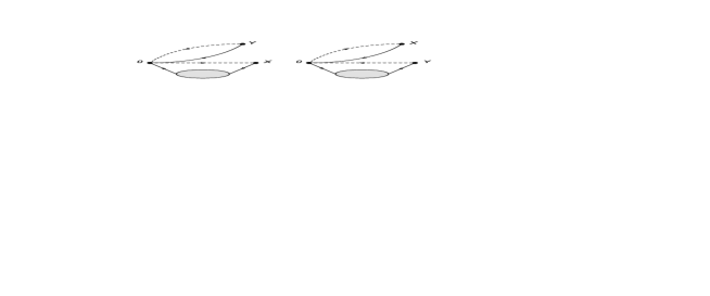
Figure 2: The lowest order Feynman diagrams, where the dashed (solid) lines denote the heavy (light) quark lines, the ovals denote the external $\pi^{+}$ meson.

We match the hadron side with the QCD side bellow the continuum thresholds $s_{0}$ and $u_{0}$ to acquire rigorous quark-hadron duality [23, 24],

$$\int_{\Delta_{s}^{2}}^{s_{0}}ds\int_{\Delta_{u}^{2}}^{u_{0}}du\frac{\rho_{QCD}(s,u)}{(s-p^{2})(u-q^{2})} = \int_{\Delta_{s}^{2}}^{s_{0}}ds\int_{\Delta_{u}^{2}}^{u_{0}}du\left[\int_{\Delta_{s}^{\prime 2}}^{\infty}ds^{\prime}\frac{\rho_{H}(s^{\prime},s,u)}{(s^{\prime}-p^{\prime 2})(s-p^{2})(u-q^{2})}\right]\,,$$ (18)

and we carry out the integral over $ds^{\prime}$ firstly, then

$$\Pi_{H}(p^{\prime 2},p^{2},q^{2}) = \frac{\lambda_{Y}f_{D^{*}}^{2}M_{D^{*}}^{2}G_{\pi/Y}}{(M_{Y}^{2}-p^{\prime 2})(M_{\bar{D}^{*}}^{2}-p^{2})(M_{D^{*}}^{2}-q^{2})}+\int_{s^{\prime}_{0}}^{\infty}ds^{\prime}\frac{\tilde{\rho}_{H}(s^{\prime},M_{\bar{D}^{*}}^{2},M_{D^{*}}^{2})}{(s^{\prime}-p^{\prime 2})(M_{\bar{D}^{*}}^{2}-p^{2})(M_{D^{*}}^{2}-q^{2})}$$ (19)

$$+\cdots\,,$$

$$= \frac{\lambda_{Y}f_{D^{*}}^{2}M_{D^{*}}^{2}G_{\pi/Y}}{(M_{Y}^{2}-p^{\prime 2})(M_{\bar{D}^{*}}^{2}-p^{2})(M_{D^{*}}^{2}-q^{2})}+\frac{C_{\pi/Y}}{(M_{\bar{D}^{*}}^{2}-p^{2})(M_{D^{*}}^{2}-q^{2})}+\cdots\,,$$

where $\rho_{H}(s^{\prime},s,u)=\tilde{\rho}_{H}(s^{\prime},s,u)\delta(s-M_{\bar{D}^{*}}^{2})\delta(u-M_{D^{*}}^{2})$, and we introduce the parameters $C_{\pi/Y}$ to parameterize the contributions concerning the higher resonances and continuum states in the $s^{\prime}$ channel,

$$C_{\pi/Y} = \int_{s^{\prime}_{0}}^{\infty}ds^{\prime}\frac{\tilde{\rho}_{H}(s^{\prime},M_{\bar{D}^{*}}^{2},M_{D^{*}}^{2})}{s^{\prime}-p^{\prime 2}}\,.$$ (20)

As the strong interactions among the ground states $\pi$, $D^{*}$, $\bar{D}^{*}$ and excited $Y^{\prime}$ states are complex, and we have no knowledge about the corresponding four-hadron contact vertex. In practical calculations, we can take the unknown functions $C_{\pi/Y}$ as free parameters and adjust the values to acquire flat platforms for the hadronic coupling constants $G_{\pi/Y}$ with variations of the Borel parameters. Such a method works well in the case of three-hadron contact vertexes [23, 24, 25, 26, 27, 28, 29], and we expect it also works in the present work.

In Eq.(5) and Eq.(8), there exist three poles in the limit $p^{\prime 2}\to M_{Y}^{2}$, $p^{2}\to M_{\bar{D}^{*}}^{2}$ and $q^{2}\to M_{D^{*}}^{2}$. According to the relation $M_{Y}\approx M_{\bar{D}^{*}}+M_{D^{*}}$, we can set $p^{\prime 2}=4q^{2}$ in the correlation functions $\Pi_{H}(p^{\prime 2},p^{2},q^{2})$, and perform double Borel transform in regard to the variables $P^{2}=-p^{2}$ and $Q^{2}=-q^{2}$ respectively, then we set the Borel parameters $T_{1}^{2}=T_{2}^{2}=T^{2}$ to acquire two QCD sum rules,

$$\frac{\lambda_{YD^{*}D^{*}}G_{\pi}}{4\left(\widetilde{M}_{Y}^{2}-M_{D^{*}}^{2}\right)}\left[\exp\left(-\frac{M_{D^{*}}^{2}}{T^{2}}\right)-\exp\left(-\frac{\widetilde{M}_{Y}^{2}}{T^{2}}\right)\right]\exp\left(-\frac{M_{\bar{D}^{*}}^{2}}{T^{2}}\right)+C_{\pi}\exp\left(-\frac{M_{D^{*}}^{2}+M_{\bar{D}^{*}}^{2}}{T^{2}}\right)$$

$$=f_{\pi}m_{c}\int_{m_{c}^{2}}^{s_{0}}ds\int_{0}^{1}du\varphi_{\pi}(u)\left[\frac{1}{2\pi^{2}}\int_{x_{i}}^{1}dxx\bar{x}(s-\tilde{m}_{c}^{2})-\left(\frac{2m_{c}\langle\bar{q}q\rangle}{3}-\frac{m_{c}^{3}\langle\bar{q}g_{s}\sigma Gq\rangle}{6T^{4}}\right)\delta(s-m_{c}^{2})\right]$$

$$\exp\left(-\frac{s+m_{c}^{2}+u\bar{u}m_{\pi}^{2}}{T^{2}}\right)$$

$$+\frac{f_{\pi}m_{\pi}^{2}}{m_{u}+m_{d}}\int_{m_{c}^{2}}^{s_{0}}ds\int_{0}^{1}du\varphi_{5}(u)\bar{u}\left[\frac{1}{2\pi^{2}}\int_{x_{i}}^{1}dxx\bar{x}(s-\tilde{m}_{c}^{2})-\left(\frac{2m_{c}\langle\bar{q}q\rangle}{3}-\frac{m_{c}^{3}\langle\bar{q}g_{s}\sigma Gq\rangle}{6T^{4}}\right)\delta(s-m_{c}^{2})\right]$$

$$\exp\left(-\frac{s+m_{c}^{2}+u\bar{u}m_{\pi}^{2}}{T^{2}}\right)+\frac{f_{\pi}m_{c}^{2}\langle\bar{q}g_{s}\sigma Gq\rangle}{36T^{2}}\int_{0}^{1}du\varphi_{\pi}(u)\exp\left(-\frac{2m_{c}^{2}+u\bar{u}m_{\pi}^{2}}{T^{2}}\right)$$

$$-\frac{f_{\pi}m_{\pi}^{2}m_{c}\langle\bar{q}g_{s}\sigma Gq\rangle}{36(m_{u}+m_{d})T^{2}}\int_{0}^{1}du\varphi_{5}(u)\bar{u}\exp\left(-\frac{2m_{c}^{2}+u\bar{u}m_{\pi}^{2}}{T^{2}}\right)\,,$$ (21)

$$\frac{\lambda_{YD^{*}D^{*}}G_{Y}}{4\left(\widetilde{M}_{Y}^{2}-M_{D^{*}}^{2}\right)}\left[\exp\left(-\frac{M_{D^{*}}^{2}}{T^{2}}\right)-\exp\left(-\frac{\widetilde{M}_{Y}^{2}}{T^{2}}\right)\right]\exp\left(-\frac{M_{\bar{D}^{*}}^{2}}{T^{2}}\right)+C_{Y}\exp\left(-\frac{M_{D^{*}}^{2}+M_{\bar{D}^{*}}^{2}}{T^{2}}\right)$$

$$=\frac{f_{\pi}m_{\pi}^{2}}{m_{u}+m_{d}}\int_{m_{c}^{2}}^{s_{0}}ds\int_{0}^{1}du\varphi_{5}(u)\left[\frac{1}{2\pi^{2}}\int_{x_{i}}^{1}dxx\bar{x}(s-\tilde{m}_{c}^{2})-\left(\frac{2m_{c}\langle\bar{q}q\rangle}{3}-\frac{m_{c}^{3}\langle\bar{q}g_{s}\sigma Gq\rangle}{6T^{4}}\right)\delta(s-m_{c}^{2})\right]$$

$$\exp\left(-\frac{s+m_{c}^{2}+u\bar{u}m_{\pi}^{2}}{T^{2}}\right)-\frac{f_{\pi}m_{\pi}^{2}m_{c}\langle\bar{q}g_{s}\sigma Gq\rangle}{36(m_{u}+m_{d})T^{2}}\int_{0}^{1}du\varphi_{5}(u)\exp\left(-\frac{2m_{c}^{2}+u\bar{u}m_{\pi}^{2}}{T^{2}}\right)$$

$$-\frac{f_{3\pi}m_{\pi}^{2}}{2\pi^{2}}\int_{m_{c}^{2}}^{s_{0}}ds\int_{x_{i}}^{1}dx\bar{x}\left[\frac{3}{4}+s\,\delta(s-\tilde{m}_{c}^{2})\right]\exp\left(-\frac{s+m_{c}^{2}}{T^{2}}\right)$$

$$-\frac{f_{3\pi}m_{\pi}^{2}}{2\pi^{2}T^{2}}\int_{m_{c}^{2}}^{s_{0}}ds\int_{x_{i}}^{1}dxx\bar{x}\,\tilde{m}_{c}^{2}\exp\left(-\frac{s+m_{c}^{2}}{T^{2}}\right)$$

$$+\frac{f_{3\pi}m_{\pi}^{2}}{4\pi^{2}}\int_{m_{c}^{2}}^{s_{0}}ds\int_{x_{i}}^{1}dxx\left[\frac{3}{2}-s\,\delta(s-\tilde{m}_{c}^{2})\right]\exp\left(-\frac{s+m_{c}^{2}}{T^{2}}\right)\,,$$ (22)

where $\lambda_{YD^{*}D^{*}}=\lambda_{Y}f_{D^{*}}^{2}M^{2}_{D^{*}}$, $\widetilde{M}_{Y}^{2}=\frac{M_{Y}^{2}}{4}$ and $x_{i}=\frac{m_{c}^{2}}{s}$. In numerical calculations, we take the $C_{\pi}$ and $C_{Y}$ as free parameters, and search for the best values to acquire stable QCD sum rules.

3 Numerical results and discussions

We take the standard values of the vacuum condensates, $\langle\bar{q}q\rangle=-(0.24\pm 0.01\,\rm{GeV})^{3}$, $\langle\bar{q}g_{s}\sigma Gq\rangle=m_{0}^{2}\langle\bar{q}q\rangle$, $m_{0}^{2}=(0.8\pm 0.1)\,\rm{GeV}^{2}$ at the energy scale $\mu=1\,\rm{GeV}$ [37, 38, 39], and take the $\overline{MS}$ mass $m_{c}(m_{c})=(1.275\pm 0.025)\,\rm{GeV}$ from the Particle Data Group [1]. We set $m_{u}=m_{d}=0$ and take account of the energy-scale dependence of the input parameters,

$$\langle\bar{q}q\rangle(\mu) = \langle\bar{q}q\rangle({\rm 1GeV})\left[\frac{\alpha_{s}({\rm 1GeV})}{\alpha_{s}(\mu)}\right]^{\frac{12}{33-2n_{f}}}\,,$$

$$\langle\bar{q}g_{s}\sigma Gq\rangle(\mu) = \langle\bar{q}g_{s}\sigma Gq\rangle({\rm 1GeV})\left[\frac{\alpha_{s}({\rm 1GeV})}{\alpha_{s}(\mu)}\right]^{\frac{2}{33-2n_{f}}}\,,$$

$$m_{c}(\mu) = m_{c}(m_{c})\left[\frac{\alpha_{s}(\mu)}{\alpha_{s}(m_{c})}\right]^{\frac{12}{33-2n_{f}}}\,,$$

$$\alpha_{s}(\mu) = \frac{1}{b_{0}t}\left[1-\frac{b_{1}}{b_{0}^{2}}\frac{\log t}{t}+\frac{b_{1}^{2}(\log^{2}{t}-\log{t}-1)+b_{0}b_{2}}{b_{0}^{4}t^{2}}\right]\,,$$ (23)

where $t=\log\frac{\mu^{2}}{\Lambda_{QCD}^{2}}$, $b_{0}=\frac{33-2n_{f}}{12\pi}$, $b_{1}=\frac{153-19n_{f}}{24\pi^{2}}$, $b_{2}=\frac{2857-\frac{5033}{9}n_{f}+\frac{325}{27}n_{f}^{2}}{128\pi^{3}}$, $\Lambda_{QCD}=210\,\rm{MeV}$, $292\,\rm{MeV}$ and $332\,\rm{MeV}$ for the flavors $n_{f}=5$, $4$ and $3$, respectively [1, 40], and we choose $n_{f}=4$.

At the hadron side, we take the parameters as $m_{\pi}=0.13957\,\rm{GeV}$, $f_{\pi}=0.130\,\rm{GeV}$ [39], $M_{D^{*}}=2.01\,\rm{GeV}$, $f_{D^{*}}=263\,\rm{MeV}$, $s^{0}_{D^{*}}=6.4\,\rm{GeV}^{2}$ [41], $M_{Y}=4.48\,\rm{GeV}$, $\lambda_{Y}=9.47\times 10^{-2}\,\rm{GeV}^{5}$ [22], and $f_{\pi}m^{2}_{\pi}/(m_{u}+m_{d})=-2\langle\bar{q}q\rangle/f_{\pi}$ from the Gell-Mann-Oakes-Renner relation.

In calculations, we fit the free parameters to be $C_{\pi}=0.00101(T^{2}-3.6\,\rm{GeV}^{2})\,\rm{GeV}^{4}$ and $C_{Y}=0.00089(T^{2}-3.2\,\rm{GeV}^{2})\,\rm{GeV}^{4}$ to acquire uniform flat Borel platforms $T^{2}_{max}-T^{2}_{min}=1\,\rm{GeV}^{2}$ (just like in our previous works [23, 24, 25, 26, 27, 28, 29]), where the max and min represent the maximum and minimum values, respectively. The Borel windows are $T^{2}_{\pi}=(4.6-5.6)\,\rm{GeV}^{2}$ and $T^{2}_{Y}=(4.4-5.4)\,\rm{GeV}^{2}$, where the subscripts $\pi$ and $Y$ represent the corresponding channels, the uncertainties $\delta G_{\pi/Y}$ come from the Borel parameters $T^{2}$ are less than $0.01\,(\rm GeV^{-1})$. In Fig.3, we plot the hadronic coupling constants $G_{\pi}$ and $G_{Y}$ with variations of the Borel parameters. In the Borel windows, there appear very flat platforms indeed, it is reasonable and reliable to extract the $G_{\pi}$ and $G_{Y}$.

If we take the symbol $\xi$ to stand for the input parameters, then the uncertainties $\bar{\xi}\to\bar{\xi}+\delta\xi$ result in the uncertainties $\bar{\lambda}_{Y}\bar{f}_{D^{*}}\bar{f}_{\bar{D}^{*}}\bar{G}_{\pi/Y}\to\bar{\lambda}_{Y}\bar{f}_{D^{*}}\bar{f}_{\bar{D}^{*}}\bar{G}_{\pi/Y}+\delta\,\bar{\lambda}_{Y}\bar{f}_{D^{*}}\bar{f}_{\bar{D}^{*}}\bar{G}_{\pi/Y}$, $\bar{C}_{\pi/Y}\to\bar{C}_{\pi/Y}+\delta C_{\pi/Y}$,

$$\delta\,\bar{\lambda}_{Y}\bar{f}_{D^{*}}\bar{f}_{\bar{D}^{*}}\bar{G}_{\pi/Y} = \bar{\lambda}_{Y}\bar{f}_{D^{*}}\bar{f}_{\bar{D}^{*}}\bar{G}_{\pi/Y}\left(\frac{\delta f_{D^{*}}}{\bar{f}_{D^{*}}}+\frac{\delta f_{\bar{D}^{*}}}{\bar{f}_{\bar{D}^{*}}}+\frac{\delta\lambda_{Y}}{\bar{\lambda}_{Y}}+\frac{\delta G_{\pi/Y}}{\bar{G}_{\pi/Y}}\right)\,,$$ (24)

where the short overline  $\bar{}$  on all the input parameters represents the central values. In calculation, we observe that the uncertainties $\delta C_{\pi/Y}$ are very small, and set $\delta C_{\pi/Y}=0$ and $\frac{\delta f_{D^{*}}}{\bar{f}_{D^{*}}}=\frac{\delta f_{\bar{D}^{*}}}{\bar{f}_{\bar{D}^{*}}}=\frac{\delta\lambda_{Y}}{\bar{\lambda}_{Y}}=\frac{\delta G_{\pi/Y}}{\bar{G}_{\pi/Y}}$ approximately. Now we obtain the hadronic coupling constants routinely,

$$G_{\pi} = 15.9\pm 0.5\,\rm{GeV}^{-1}\,,$$

$$G_{Y} = 10.4\pm 0.6\,\rm{GeV}^{-1}\,,$$ (25)

by setting

$$\delta\,\bar{\lambda}_{Y}\bar{f}_{D^{*}}\bar{f}_{\bar{D}^{*}}\bar{G}_{\pi/Y} = \bar{\lambda}_{Y}\bar{f}_{D^{*}}\bar{f}_{\bar{D}^{*}}\bar{G}_{\pi/Y}\frac{4\delta G_{\pi/Y}}{\bar{G}_{\pi/Y}}\,.$$ (26)

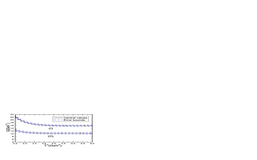
Figure 3: The hadronic coupling constants with variations of the Borel parameters $T^{2}$, where the (I) and (II) denote the $G_{\pi}$ and $G_{Y}$, respectively, the regions between the two vertical lines are the Borel windows.

Then it is direct to obtain the partial decay width by taking the hadron masses $M_{D^{*-}}=2.01026\,\rm{GeV}$, $M_{D^{*0}}=2.00685\,\rm{GeV}$ and $m_{\pi}=0.13957\,\rm{GeV}$ from the Particle Data Group [1] and $M_{Y(4500)}=4.4691\,\rm{GeV}$ from the BESIII collaboration [9],

$$\Gamma\left(Y(4500)\to D^{*}\bar{D}^{*}\pi^{+}\right) = \frac{1}{24\pi M_{Y}}\int dk^{2}(2\pi)^{4}\delta^{4}(p^{\prime}-k-p)\frac{d^{3}\vec{k}}{(2\pi)^{3}2k_{0}}\frac{d^{3}\vec{p}}{(2\pi)^{3}2p_{0}}$$ (27)

$$(2\pi)^{4}\delta^{4}(k-q-r)\frac{d^{3}\vec{q}}{(2\pi)^{3}2q_{0}}\frac{d^{3}\vec{r}}{(2\pi)^{3}2r_{0}}\Sigma|T|^{2}$$

$$= 6.43^{+0.80}_{-0.76}\,\rm{MeV}\,,$$

where $T=\langle Y_{c}(p^{\prime})|\bar{D}^{*}(p)D^{*}(q)\pi(r)\rangle$ defined in Eq.(7).

The partial decay width $\Gamma\left(Y(4500)\to D^{*}\bar{D}^{*}\pi^{+}\right)=6.43^{+0.80}_{-0.76}\,\rm{MeV}$ is much smaller than the total width $\Gamma=246.3\pm 36.7\pm 9.4\,\rm{MeV}$ from the BESIII collaboration [9], which is consistent with our naive expectation that the main decay channels of the vector tetraquark states are two-body strong decays $Y\to D\bar{D}$, $D^{*}\bar{D}^{*}$, $D\bar{D}^{*}$, $D^{*}\bar{D}$, $J/\psi\pi$, $\eta_{c}\rho$. The observations of the $Y(4500)$ in the channels $D\bar{D}$, $D^{*}\bar{D}^{*}$, $D\bar{D}^{*}$, $D^{*}\bar{D}$, $J/\psi\pi$, $\eta_{c}\rho$ would shed light on the nature of the $Y(4500)$, and we would explore those two-body strong decays in our next work in a comprehensive way.

We choose the process $Y(4500)\to D^{*-}D^{*0}\pi^{+}$ to explore whether or not the four-hadron coupling constants can be calculated directly using the (light-cone) QCD sum rules, as this process is not expected to be the dominant decay channel, which only servers as a powerful constraint to examine the calculations, i.e. the partial decay width should be small enough to satisfy the BESIII experimental data. We should admit that it would be better to find a tetraquark candidate, whose dominant decay mode is the three-body strong decay, to examine the present approach (or procedure), however, at the present time, we cannot find such a tetraquark candidate. In short, the present work supports assigning the $Y(4500)$ to be the $[uc]_{\tilde{A}}[\overline{uc}]_{V}+[uc]_{V}[\overline{uc}]_{\tilde{A}}+[dc]_{\tilde{A}}[\overline{dc}]_{V}+[dc]_{V}[\overline{dc}]_{\tilde{A}}$ hidden-charm tetraquark state with the quantum numbers $J^{PC}=1^{--}$. It is the first time to use the light-cone QCD sum rules to study the four-hadron coupling constants, the approach can be used to explore the $Y\to J/\psi\pi^{+}\pi^{-}$, $\psi^{\prime}\pi^{+}\pi^{-}$, $J/\psi K^{+}K^{-}$, $h_{c}\pi^{+}\pi^{-}$, $D^{0}D^{*-}\pi^{+}$, and diagnose the nature of the $X$, $Y$ and $Z$ states.

4 Conclusion

In this work, we tentatively assign the $Y(4500)$ as the $[uc]_{\tilde{A}}[\overline{uc}]_{V}+[uc]_{V}[\overline{uc}]_{\tilde{A}}+[dc]_{\tilde{A}}[\overline{dc}]_{V}+[dc]_{V}[\overline{dc}]_{\tilde{A}}$ tetraquark state with the quantum numbers $J^{PC}=1^{--}$, and extend our previous works to study the three-body strong decay $Y(4500)\to D^{*-}D^{*0}\pi^{+}$ with the light-cone QCD sum rules, the partial width is consistent with the experimental data from the BESIII collaboration. It is the first time to use the light-cone QCD sum rules to study the four-hadron coupling constants, we choose the process $Y(4500)\to D^{*-}D^{*0}\pi^{+}$ to explore whether or not the (light-cone) QCD sum rules can be used to calculate the four-hadron coupling constants directly, as the process is not the main decay channel, which servers as a powerful constraint to testify the approach, i.e. the partial decay width should be small enough to be match the experimental data. The approach can be used to investigate the three-body strong decays $X/Y\to J/\psi\pi^{+}\pi^{-}$, $\psi^{\prime}\pi^{+}\pi^{-}$, $J/\psi K^{+}K^{-}$, $h_{c}\pi^{+}\pi^{-}$, $D^{0}D^{*-}\pi^{+}$ directly, and shed light on the nature of the $X$, $Y$ and $Z$ states.

References

[1] R. L. Workman et al, Prog. Theor. Exp. Phys. 2022 (2022) 083C01.
[2] B. Aubert et al, Phys. Rev. Lett. 95 (2005) 142001.
[3] M. Ablikim et al, Phys. Rev. Lett. 118 (2017) 092002.
[4] M. Ablikim et al, Phys. Rev. Lett. 118 (2017) 092001.
[5] X. L. Wang et al, Phys. Rev. Lett. 99 (2007) 142002.
[6] X. L. Wang et al, Phys. Rev. D91 (2015) 112007.
[7] G. Pakhlova et al, Phys. Rev. Lett. 101 (2008) 172001.
[8] M. Ablikim et al, Chin. Phys. C46 (2022) 111002.
[9] M. Ablikim et al, Phys. Rev. Lett. 130 (2023) 121901.
[10] M. Ablikim et al, Phys. Rev. Lett. 122 (2019) 102002.
[11] R. M. Albuquerque and M. Nielsen, Nucl. Phys. A815 (2009) 532009; Erratum-ibid. A857 (2011) 48.
[12] W. Chen and S. L. Zhu, Phys. Rev. D83 (2011) 034010.
[13] Z. G. Wang, Eur. Phys. J. C78 (2018) 518.
[14] Z. G. Wang, Eur. Phys. J. C74 (2014) 2874.
[15] Z. G. Wang, Eur. Phys. J. C76 (2016) 387.
[16] J. R. Zhang and M. Q. Huang, Phys. Rev. D83 (2011) 036005.
[17] J. R. Zhang and M. Q. Huang, JHEP 1011 (2010) 057.
[18] Z. G. Wang, Eur. Phys. J. C78 (2018) 933.
[19] Z. G. Wang, Eur. Phys. J. C79 (2019) 29.
[20] Z. G. Wang, Commun. Theor. Phys. 71 (2019) 1319.
[21] H. Sundu, S. S. Agaev and K. Azizi, Phys. Rev. D98 (2018) 054021.
[22] Z. G. Wang, Nucl. Phys. B973 (2021) 115592.
[23] Z. G. Wang and J. X. Zhang, Eur. Phys. J. C78 (2018) 14.
[24] Z. G. Wang, Eur. Phys. J. C79 (2019) 184.
[25] Z. G. Wang and Z. Y. Di, Eur. Phys. J. C79 (2019) 72.
[26] Z. G. Wang, Acta Phys. Polon. B51 (2020) 435.
[27] Z. G. Wang, Int. J. Mod. Phys. A34 (2019) 1950110.
[28] Z. G. Wang, Chin. Phys. C46 (2022) 103106.
[29] Z. G. Wang, Chin. Phys. C46 (2022) 123106.
[30] J. M. Dias, F. S. Navarra, M. Nielsen and C. M. Zanetti,
Phys. Rev. D88 (2013) 016004.
[31] W. Chen, T. G. Steele, H. X. Chen and S. L. Zhu, Eur. Phys. J. C75 (2015) 358.
[32] H. Sundu, S. S. Agaev and K. Azizi, Eur. Phys. J. C79 (2019) 215.
[33] P. Ball, JHEP 9901 (1999) 010.
[34] Z. G. Wang and S. L. Wan, Phys. Rev. D74 (2006) 014017.
[35] Z. G. Wang, J. Phys. G34 (2007) 753.
[36] V. M. Braun and I. E. Filyanov, Z. Phys. C48 (1990) 239.
[37] M. A. Shifman, A. I. Vainshtein and V. I. Zakharov, Nucl. Phys. B147 (1979) 385;
Nucl. Phys. B147 (1979) 448.
[38] L. J. Reinders, H. Rubinstein and S. Yazaki, Phys. Rept. 127 (1985) 1.
[39] P. Colangelo and A. Khodjamirian, hep-ph/0010175.
[40] S. Narison and R. Tarrach, Phys. Lett. 125 B (1983) 217.