The Global Active Subspace Method

Abstract

We present a new dimension reduction method called the global active subspace method. The method uses expected values of finite differences of the underlying function to identify the important directions, and builds a surrogate model using the important directions on a lower dimensional subspace. The method is a generalization of the active subspace method which uses the gradient information of the function to construct a reduced model. We develop the error analysis for the global active subspace method, and present examples to compare it with the active subspace method numerically. The results show that the global active subspace method is accurate, efficient, and robust with respect to noise or lack of smoothness in the underlying function.

65C05, 65C20, 65C60

1 Introduction

The active subspace (AS) method is a dimension reduction method introduced in Constantine et al. [5], and further developed in Constantine [4] and Constantine and Gleich [8]. The method has been applied successfully in many problems in fields of engineering, public health, quantitative finance, and geosciences (see Constantine et al. [7], Cui et al. [9], Demo et al. [10], Diaz et al. [11], Jefferson et al. [21], Kubler and Scheidegger[22], Li et al. [24], Liu and Owen [25], Lukaczyk et al. [26], Zhou and Peng [41]). The method uses the gradient information of a function to find the directions along which the function changes the most. The function is then approximated by one that depends only on the few important directions. Estimating the gradient accurately is crucial in successful application of the AS method, and several researchers introduced methods for this estimation, for example, Coleman et al. [3], Constantine et al. [6], Lewis et al. [23], Ma et al. [28], Navaneeth and Chakraborty [31], Wycoff et al. [38], and Yan et al. [40].

In this paper we will introduce a generalization of the AS method, called the global active subspace method (GAS), that does not rely on gradients. Instead the method computes the expectations of first order finite-differences of function values, and uses this information to identify the important directions along which the function changes the most. The GAS method measures change in function values in a global way by considering finite-differences as opposed to partial derivatives, and it has theoretical connections with Sobol’ sensitivity indices (Sobol’ [36]), a popular measure used in global sensitivity analysis (Saltelli et al. [33]). We will use numerical results to demonstrate the effectiveness of the GAS method when the underlying function is noisy or lacks the necessary smoothness.

The paper is organized as follows. Section 2 presents the definition of the GAS method, discusses some computational issues, and describes how to build a surrogate model using the GAS method. Section 2.4 presents an algorithm for the method. The error analysis of the method is established in Sections 3 and 4. Several numerical examples are used to compare the accuracy and efficiency of the AS and GAS methods in Section 5. We conclude in Section 6.

2 Global Active Subspace Method

In this section we develop the theoretical foundation of the global active subspace (GAS) method, discuss computational issues and construction of surrogate models based on the important directions, and present its algorithm.

2.1 Derivation of GAS Method

Consider a square-integrable real-valued function $f(\boldsymbol{z})$ with domain $\Omega\subset\boldsymbol{R}^{d}$ and finite second-order partial derivatives. Suppose that $\Omega$ is equipped with a probability measure with a cumulative distribution function in the form $\boldsymbol{F}(\boldsymbol{z})=F_{1}(z_{1})\cdot\ldots\cdot F_{d}(z_{d})$, where $F_{i}$ are marginal distribution functions.

We define a vector function $D_{\boldsymbol{z}}f:\Omega\times\Omega\rightarrow\boldsymbol{R}^{d}$ as follows:

$$D_{\boldsymbol{z}}f(\boldsymbol{v},\boldsymbol{z})=[D_{\boldsymbol{z},1}f(v_{1},\boldsymbol{z}),\ldots,D_{\boldsymbol{z},d}f(v_{d},\boldsymbol{z})]^{T},$$

where

(1) $$D_{\boldsymbol{z},i}f(v_{i},\boldsymbol{z})=(f(\boldsymbol{v}_{\{i\}},\boldsymbol{z}_{-\{i\}})-f(\boldsymbol{z}))/(v_{i}-z_{i}).$$

Here $\boldsymbol{v}_{\{i\}}$ corresponds to the $i$th input of vector $\boldsymbol{v}$, and $\boldsymbol{z}_{-\{i\}}$ is the vector of inputs corresponding to those indices in the complement of $\{i\}$. In this way, $(\boldsymbol{v}_{\{i\}},\boldsymbol{z}_{-\{i\}})$ is the vector that changes the $i$th input of $\boldsymbol{z}$ to $v_{i}$, while keeping the other inputs of $\boldsymbol{z}$ the same.

Define the $d\times d$ matrix $\boldsymbol{C}$ by

(2) $$\boldsymbol{C}={\rm E}\,[{\rm E}\,[(D_{\boldsymbol{z}}f)(D_{\boldsymbol{z}}f)^{T}|\boldsymbol{z}]],$$

where the inner conditional expectation fixes $\boldsymbol{z}$ and averages over the components of $\boldsymbol{v}=[v_{1},\ldots,v_{d}]^{T}$, and the outside expectation averages with respect to $\boldsymbol{z}$.

To get a better understanding of the matrix $\boldsymbol{C}$ let us consider a simple example, a two dimensional function $f(z_{1},z_{2})$. The vector function $D_{\boldsymbol{z}}f$ is then

(3) $$D_{\boldsymbol{z}}f(\boldsymbol{v},\boldsymbol{z})=\left[\frac{f(v_{1},z_{2})-f(z_{1},z_{2})}{v_{1}-z_{1}},\frac{f(z_{1},v_{2})-f(z_{1},z_{2})}{v_{2}-z_{2}}\right]^{T},$$

and the matrix $\boldsymbol{C}$ is

(4) $$\boldsymbol{C}=\left[\begin{array}[]{cc}C_{11}&C_{12}\\ C_{21}&C_{22}\end{array}\right],$$

where

$$\begin{split}C_{11}&=\int\int\frac{(f(v_{1},z_{2})-f(z_{1},z_{2}))^{2}}{(v_{1}-z_{1})^{2}}dF_{1}(v_{1})d\boldsymbol{F}(\boldsymbol{z}),\\ C_{22}&=\int\int\frac{(f(z_{1},v_{2})-f(z_{1},z_{2}))^{2}}{(v_{2}-z_{2})^{2}}dF_{2}(v_{2})d\boldsymbol{F}(\boldsymbol{z}),\\ C_{12}=C_{21}&=\int\int\frac{(f(v_{1},z_{2})-f(z_{1},z_{2}))(f(z_{1},v_{2})-f(z_{1},z_{2}))}{(v_{1}-z_{1})(v_{2}-z_{2})}dF_{1}(v_{1})dF_{2}(v_{2})d\boldsymbol{F}(\boldsymbol{z}).\end{split}$$

The matrix $\boldsymbol{C}$ provides a global measure of change for the function $f$, and it resembles upper Sobol’ sensitivity indices (Sobol’ [36]), which is a popular measure used in global sensitivity analysis. Recall that the first-order upper Sobol’ sensitivity indices can be written as (Saltelli et al. [32])

(5) $$\bar{S}_{i}=\frac{1}{2\sigma^{2}}\int{(f(\boldsymbol{v}_{\{i\}},\boldsymbol{z}_{-\{i\}})-f(\boldsymbol{z}))^{2}d\boldsymbol{F}(\boldsymbol{z})dF_{i}(v_{i})},$$

where $\sigma^{2}$ is the variance of $f$. If we did not divide $f(\boldsymbol{v}_{\{i\}},\boldsymbol{z}_{-\{i\}})-f(\boldsymbol{z})$ by $v_{i}-z_{i}$ in the definition of $D_{\boldsymbol{z}}f(\boldsymbol{z})$ (Eqn. 1), then the diagonal elements of $\frac{1}{2\sigma^{2}}\boldsymbol{C}$ would be exactly the upper Sobol’ indices $\bar{S}_{1},\ldots,\bar{S}_{d}$.

The active subspace method also constructs a matrix $\boldsymbol{C}$, where the matrix is obtained from the gradient of $f$. While the active subspace method uses local information about the change in function values (partial derivatives), our proposed approach uses a global measure of change in the function values (like Sobol’ sensitivity indices). We will illustrate the benefits of this new approach in the numerical results.

Like in the active subspace method, we will use the eigenvalue decomposition of $\boldsymbol{C}$ to find the important variables, or directions, of $f$. As $\boldsymbol{C}$ is symmetric and positive semi-definite, there exists a real eigenvalue decomposition. To this end, consider the eigenvalue decomposition of $\boldsymbol{C}$:

(6) $$\boldsymbol{C}=\boldsymbol{U}\Lambda\boldsymbol{U}^{T},\Lambda=diag(\lambda_{1},\ldots,\lambda_{d}),\lambda_{1}\geq\ldots\geq\lambda_{d}\geq 0.$$

Partition the eigenvalues and eigenvectors as follows:

(7) $$\Lambda=\left[\begin{array}[]{cc}\Lambda_{1}&\\ &\Lambda_{2}\end{array}\right],\boldsymbol{U}=\left[\begin{array}[]{cc}\boldsymbol{U}_{1}&\boldsymbol{U}_{2}\end{array}\right],$$

where $\Lambda_{1}=diag(\lambda_{1},\ldots,\lambda_{d_{1}})$ with $d_{1}<d$, and $\boldsymbol{U}_{1}\in\boldsymbol{R}^{d\times d_{1}}$. Introduce new variables (rotated coordinates), $\boldsymbol{w}_{1},\boldsymbol{w}_{2}$ as:

(8) $$\boldsymbol{w}_{1}=\boldsymbol{U}_{1}^{T}\boldsymbol{z}\in\boldsymbol{R}^{d_{1}},\boldsymbol{w}_{2}=\boldsymbol{U}_{2}^{T}\boldsymbol{z}\in\boldsymbol{R}^{d-d_{1}}.$$

The vector $\boldsymbol{w}_{1}$, obtained through eigenvectors corresponding to larger eigenvalues, holds the information about the important directions for the function $f$. These are the directions along which the function changes the most. We will call the subspace generated by directions in $\boldsymbol{w}_{1}$, the global active subspace. Directions in the other vector $\boldsymbol{w}_{2}$ are unimportant; the function does not change as much along those directions. The theoretical justification for these statements is based on the following lemma.

Lemma 2.1.

For a square-integrable function $f(\boldsymbol{z})$ with finite second-order partial derivatives, we have

$${\rm E}\,[{\rm E}\,[(D_{\boldsymbol{w}_{1}}f)^{T}(D_{\boldsymbol{w}_{1}}f)|\boldsymbol{w}_{1}]]=\lambda_{1}+\ldots+\lambda_{d_{1}}+C_{U_{1}},$$

$${\rm E}\,[{\rm E}\,[(D_{\boldsymbol{w}_{2}}f)^{T}(D_{\boldsymbol{w}_{2}}f)|\boldsymbol{w}_{2}]]=\lambda_{d_{1}+1}+\ldots+\lambda_{d}+C_{U_{2}},$$

where $C_{U_{1}},C_{U_{2}}$ are two constants related to the matrix $\boldsymbol{U}$ and the second order derivatives of $f$.

Proof 2.2.

We have

(9) $$f(\boldsymbol{z})=f(\boldsymbol{U}\boldsymbol{U}^{T}\boldsymbol{z})=f(\boldsymbol{U}_{1}\boldsymbol{U}_{1}^{T}\boldsymbol{z}+\boldsymbol{U}_{2}\boldsymbol{U}_{2}^{T}\boldsymbol{z})=f(\boldsymbol{U}_{1}\boldsymbol{w}_{1}+\boldsymbol{U}_{2}\boldsymbol{w}_{2}).$$

We then derive the following equations:

(10) $$\begin{split}&D_{\boldsymbol{z}}f=\nabla_{\boldsymbol{z}}f(\boldsymbol{z})+R_{1}(\boldsymbol{z}-\boldsymbol{v}),\\ &D_{\boldsymbol{w}_{1}}f=\boldsymbol{U}_{1}^{T}\nabla_{\boldsymbol{z}}f(\boldsymbol{z})+R_{1}(\boldsymbol{U}_{1}^{T}(\boldsymbol{z}-\boldsymbol{v})),\end{split}$$

where $R_{1}(\boldsymbol{z}-\boldsymbol{v})$ and $R_{1}(\boldsymbol{U}_{1}^{T}(\boldsymbol{z}-\boldsymbol{v}))$ are two vectors obtained from the remainder terms of Taylor expansions.

To derive the first equation of Eqn. (10), we write the Taylor expansion for $f(\boldsymbol{v}_{\{i\}},\boldsymbol{z}_{-\{i\}})$ at the point $\boldsymbol{z}$ for each $i$, then approximate each entry in the vector $D_{\boldsymbol{z}}f$ with the Taylor expansion, and summarize the result in the vector form. To prove the second line of Eqn. (10), we write the Taylor expansion for each entry in the vector $D_{\boldsymbol{w}_{1}}f$, and then rewrite the expression using $\boldsymbol{v}$ and $\boldsymbol{z}$ to get the result.

Then

$${\rm E}\,[{\rm E}\,[(D_{\boldsymbol{w}_{1}}f)^{T}(D_{\boldsymbol{w}_{1}}f)|\boldsymbol{w}_{1}]]={\rm E}\,[{\rm E}\,[trace((D_{\boldsymbol{w}_{1}}f)(D_{\boldsymbol{w}_{1}}f)^{T})|\boldsymbol{w}_{1}]]$$

$$=trace({\rm E}\,[{\rm E}\,[(D_{\boldsymbol{w}_{1}}f)(D_{\boldsymbol{w}_{1}}f)^{T}|\boldsymbol{z}]])$$

$$=trace({\rm E}\,[{\rm E}\,[\boldsymbol{U}_{1}^{T}(D_{\boldsymbol{z}}f)(D_{\boldsymbol{z}}f)^{T}\boldsymbol{U}_{1}|\boldsymbol{z}]])+trace({\rm E}\,[2\boldsymbol{U}_{1}^{T}(D_{\boldsymbol{z}}f)\boldsymbol{a}^{T}+\boldsymbol{aa}^{T}])$$

$$=\lambda_{1}+\ldots+\lambda_{d_{1}}+C_{U_{1}},$$

where

$$D_{\boldsymbol{w}_{1}}f =\boldsymbol{U}_{1}^{T}D_{\boldsymbol{z}}f+\boldsymbol{a}$$

$$\boldsymbol{a} =R_{1}(\boldsymbol{U}_{1}^{T}(\boldsymbol{z}-\boldsymbol{v}))-\boldsymbol{U}_{1}^{T}R_{1}(\boldsymbol{z}-\boldsymbol{v})$$

$$C_{U_{1}} =trace({\rm E}\,[2\boldsymbol{U}_{1}^{T}(D_{\boldsymbol{z}}f)\boldsymbol{a}^{T}+\boldsymbol{aa}^{T}]).$$

The second equation of the lemma can be derived similarly, and we get

$$\boldsymbol{a}^{\prime} =R_{1}(\boldsymbol{U}_{2}^{T}(\boldsymbol{z}-\boldsymbol{v}))-\boldsymbol{U}_{2}^{T}R_{1}(\boldsymbol{z}-\boldsymbol{v})$$

$$C_{U_{2}} =trace({\rm E}\,[2\boldsymbol{U}_{2}^{T}(D_{\boldsymbol{z}}f)\boldsymbol{a}^{\prime T}+\boldsymbol{a}^{\prime}\boldsymbol{a}^{\prime T}]).$$

Remark 2.3.

It is interesting to compare Lemma 2.1 to a similar result for the active subspace method (Lemma 2.2 of [5]). In the active subspace method, there are no constant terms in the right-hand sides of the expectations. These constants appear as we generalize the approach from gradients to first-order divided differences. Lemma 2.1 shows that when $\lambda_{d_{1}+1}+\ldots+\lambda_{d}+C_{U_{2}}$ is small, the changes for function $f$ along the directions in $\boldsymbol{w}_{2}$ are also small, and thus we can focus on the global active subspace formed by directions in $\boldsymbol{w}_{1}$. In our numerical implementations, we typically make the decision on the value of $d_{1}$ by comparing the sum of the eigenvalues $\lambda_{1}+\ldots+\lambda_{d_{1}}$ and $\lambda_{d_{1}+1}+\ldots+\lambda_{d}$, ignoring the constants $C_{U_{1}}$ and $C_{U_{2}}$.

After the global active subspace is determined, the next task is to approximate $f$ by a function that only depends on the variables in the global active subspace, $\boldsymbol{w}_{1}$. This is done in a similar way to the active subspace method, by integrating out the “unimportant” variables $\boldsymbol{w}_{2}$ using conditional expectations. Let $\rho$ be the probability density function that corresponds to the distribution function $\boldsymbol{F}$. Let the joint probability density of $\boldsymbol{w}_{1},\boldsymbol{w}_{2}$ to be $\pi(\boldsymbol{w}_{1},\boldsymbol{w}_{2})=\rho({\boldsymbol{U}}_{1}\boldsymbol{w}_{1}+{\boldsymbol{U}}_{2}\boldsymbol{w}_{2})$, and the conditional probability density of $\boldsymbol{w}_{2}$ given $\boldsymbol{w}_{1}$ to be $\pi_{\boldsymbol{w}_{2}|\boldsymbol{w}_{1}}$, then

(11) $$f(\boldsymbol{z})\approx F(\boldsymbol{z})=G(\boldsymbol{w}_{1})=\int{f({\boldsymbol{U}}_{1}\boldsymbol{w}_{1}+{\boldsymbol{U}}_{2}\boldsymbol{u})\pi_{\boldsymbol{w}_{2}|\boldsymbol{w}_{1}}}(\boldsymbol{u}|\boldsymbol{w}_{1})d\boldsymbol{u}.$$

Note that when $\boldsymbol{z}\sim\mathcal{N}(\boldsymbol{0},\boldsymbol{I_{d}})$, we have $\pi_{\boldsymbol{w}_{2}|\boldsymbol{w}_{1}}=\pi_{\boldsymbol{w}_{2}}$. For this convenience we prefer to use normal distribution when sampling from $\boldsymbol{z}$ in the numerical results.

2.2 Computational Issues

To estimate $\boldsymbol{C}$, we use the Monte Carlo method:

(12) $$\hat{\boldsymbol{C}}=\frac{1}{M_{1}M_{2}}\sum_{i=1}^{M_{1}}\sum_{j=1}^{M_{2}}(D_{\boldsymbol{z}^{(i)}}f(\boldsymbol{v}^{(i,j)},\boldsymbol{z}^{(i)}))(D_{\boldsymbol{z}^{(i)}}f(\boldsymbol{v}^{(i,j)},\boldsymbol{z}^{(i)}))^{T},$$

where $\boldsymbol{z}^{(i)}$’s and $\boldsymbol{v}^{(i,j)}$’s are sampled independently from their corresponding distributions. Then we compute the eigenvalue decomposition

(13) $$\hat{\boldsymbol{C}}=\hat{\boldsymbol{U}}\hat{\Lambda}\hat{\boldsymbol{U}}^{T}.$$

An alternative and computationally more efficient way to obtain $\hat{\boldsymbol{U}}$ is by computing the singular value decomposition (SVD):

(14) $$\begin{aligned} \hat{\boldsymbol{C}}^{\frac{1}{2}}=\frac{1}{\sqrt{M_{1}M_{2}}}[&D_{\boldsymbol{z}^{(1)}}f(\boldsymbol{v}^{(1,1)},\boldsymbol{z}^{(1)}),\ldots,D_{\boldsymbol{z}^{(1)}}f(\boldsymbol{v}^{(1,M_{2})},\boldsymbol{z}^{(1)}),\\ &D_{\boldsymbol{z}^{(2)}}f(\boldsymbol{v}^{(2,1)},\boldsymbol{z}^{(2)}),\ldots,D_{\boldsymbol{z}^{(2)}}f(\boldsymbol{v}^{(2,M_{2})},\boldsymbol{z}^{(2)}),\\ &\ldots\\ &D_{\boldsymbol{z}^{(M_{1})}}f(\boldsymbol{v}^{(M_{1},1)},\boldsymbol{z}^{(M_{1})}),\ldots,D_{\boldsymbol{z}^{(M_{1})}}f(\boldsymbol{v}^{(M_{1},M_{2})},\boldsymbol{z}^{(M_{1})})]\\ =\hat{\boldsymbol{U}}\hat{\boldsymbol{\Lambda}}^{\frac{1}{2}}\hat{\boldsymbol{V}}^{T}.&\end{aligned}$$

Note that here $\hat{\boldsymbol{C}}^{\frac{1}{2}}$ is a $d\times M_{1}M_{2}$ matrix. For each $\boldsymbol{z}^{(i)})$, there are $M_{2}$ vectors shown as $M_{2}$ columns in $\hat{\boldsymbol{C}}^{\frac{1}{2}}$.

Using $\hat{\boldsymbol{U}}$ we compute estimates for $\boldsymbol{w}_{1}$, $\boldsymbol{w}_{2}$, and their probability density functions: $\hat{\boldsymbol{w}}_{1}=\hat{\boldsymbol{U}}^{T}_{1}\boldsymbol{z},\hat{\boldsymbol{w}}_{2}=\hat{\boldsymbol{U}}^{T}_{2}\boldsymbol{z}$, $\hat{\pi}(\hat{\boldsymbol{w}}_{1},\hat{\boldsymbol{w}}_{2})=\rho(\hat{\boldsymbol{U}}_{1}\hat{\boldsymbol{w}}_{1}+\hat{\boldsymbol{U}}_{2}\hat{\boldsymbol{w}}_{2})$ and $\hat{\pi}_{\hat{\boldsymbol{W}}_{2}|\hat{\boldsymbol{W}}_{1}}$. We approximate $f(\boldsymbol{z})$ by

(15) $$f(\boldsymbol{z})\approx\hat{F}(\boldsymbol{z})=\hat{G}(\hat{\boldsymbol{w}}_{1})=\int{f(\hat{\boldsymbol{U}}_{1}\hat{\boldsymbol{w}}_{1}+\hat{\boldsymbol{U}}_{2}\boldsymbol{u})\hat{\pi}_{\hat{\boldsymbol{W}}_{2}|\hat{\boldsymbol{W}}_{1}}}(\boldsymbol{u}|\hat{\boldsymbol{w}}_{1})d\boldsymbol{u}.$$

Monte Carlo is used to estimate the integral in Eqn. (15):

(16) $$\hat{F}_{mc}(\boldsymbol{z})=\hat{G}_{mc}(\hat{\boldsymbol{w}}_{1})=\frac{1}{N_{1}}\sum_{i=1}^{N_{1}}f(\hat{\boldsymbol{U}}_{1}\hat{\boldsymbol{w}}_{1}+\hat{\boldsymbol{U}}_{2}\boldsymbol{\hat{u}}^{(i)}),$$

where $\boldsymbol{\hat{u}}^{(i)}$’s are sampled from $\hat{\pi}_{\hat{\boldsymbol{W}}_{2}|\hat{\boldsymbol{W}}_{1}}$.

2.3 Surrogate Model Construction

We started with $f(\boldsymbol{z})$, discovered the global active subspace directions $\boldsymbol{w}_{1}$, and approximated $f(\boldsymbol{z})$ with $\hat{F}(\boldsymbol{z})=\hat{G}(\hat{\boldsymbol{w}}_{1})$ via Eqn. (15). The next step is to replace $\hat{F}(\boldsymbol{z})=\hat{G}(\hat{\boldsymbol{w}}_{1})$ by a surrogate model that will enable its efficient computation. Among several choices in the literature, we use polynomial chaos expansion (PCE) (Xiu and Karniadakis [39]) for this purpose.

The PCE of a square-integrable variable $Y=f(\boldsymbol{z})$ is,

$$f(\boldsymbol{z})=\sum_{i=0}^{\infty}{k_{i}\phi_{i}(\boldsymbol{z})}.$$

Here $\{\phi_{i}\}_{i=0}^{\infty}$ is a family of multidimensional orthonormal polynomials with respect to a weight function. Xiu and Karniadakis [39] introduced the Askey scheme for choosing the orthonormal polynomials. They showed it is optimal to choose the weight function to be the same as the probability density function of $\boldsymbol{z}$. If $\boldsymbol{z}$ has the uniform distribution on $[0,1]^{d}$, we pick multidimensional Legendre polynomials as the basis polynomials. If $\boldsymbol{z}$ follows the multivariate normal distribution, the multidimensional Hermite polynomials are used.

In practice, one needs to estimate the coefficients $k_{i}$, and compute

(17) $$\hat{f}_{p}(\boldsymbol{z})=\sum_{i=0}^{P-1}{\hat{k}_{i}\phi_{i}(\boldsymbol{z})},$$

where $P=\binom{d+p}{d}$ is the number of terms in the summation, and $\hat{k}_{i}$ is the estimated value for $k_{i}$. A popular method in the literature to estimate $\hat{k}_{i}$ is the least squares method. Let $\boldsymbol{\Psi}\in\boldsymbol{R}^{N\times P}$ be the coefficient matrix with $\Psi_{ni}=\phi_{i}(\boldsymbol{z}^{(n)})$, and $\boldsymbol{y}\in\boldsymbol{R}^{N}$ be the response vector with $y_{n}=f(\boldsymbol{z}^{(n)})$. The least squares approach computes

(18) $$\hat{\boldsymbol{k}}=(\boldsymbol{\Psi}^{T}\boldsymbol{\Psi})^{-1}\boldsymbol{\Psi}^{T}\boldsymbol{y},$$

which minimizes the mean square error $||\boldsymbol{y}-\boldsymbol{\Psi}\boldsymbol{k}||^{2}$.

Let $\hat{F}_{sgt}$ denote the surrogate model approximation to $\hat{F}(\boldsymbol{z})$, or more accurately, to $\hat{F}_{mc}$ (Eqn. (16)). We will assume that $\hat{F}_{sgt}$ can be made arbitrarily close to $\hat{F}_{mc}$ in the following sense.

For any $\kappa_{1}>0$, we can choose the parameters of the surrogate model so that

(19) $${\rm E}\,[(\hat{F}_{sgt}-\hat{F}_{mc})^{2}]^{\frac{1}{2}}\leq\kappa_{1}.$$

In our numerical results we use PCE with the least squares method to construct $\hat{F}_{sgt}$, and in that case a bound similar to Assumption 2.3 holds with a large probability when $N$ and $p$ are large (see Hampton and Doostan [15] for details). The deterministic error bound in the assumption allows us to combine several deterministic error bounds together to derive an error bound for ${\rm E}\,[(\hat{F}_{sgt}-f)^{2}]^{\frac{1}{2}}$ in Theorem 3.10 of Section 3.

2.4 The GAS Algorithm

Algorithm 1 is a summary of steps that starts with the function $f(\boldsymbol{z})$, finds the global active subspace, computes the surrogate model via PCE, and returns ${\rm E}\,[f(\boldsymbol{z})]$. There is nothing special about the output, ${\rm E}\,[f(\boldsymbol{z})]$, except that in the numerical results we will be comparing different methods by their root mean square error when they estimate ${\rm E}\,[f(\boldsymbol{z})]$. A computer code for this algorithm is available at: https://github.com/RuilongYue/global-active-subspace.

As discussed in Section 2.1, we assume $\boldsymbol{z}$ follows $\mathcal{N}(\boldsymbol{0},\boldsymbol{I_{d}})$ so that we can obtain $\pi(\boldsymbol{w}_{2}|\boldsymbol{w}_{1})$ easily. If $\boldsymbol{z}$ follows another distribution, we can apply transformation techniques to change the problem to one with normal distribution.

Algorithm 1 GAS_PCE Algorithm

      Input: $f(\boldsymbol{z})$ with $\boldsymbol{z}\sim\mathcal{N}(\boldsymbol{0},\boldsymbol{I_{d}})$, $K,M_{1},M_{2},N,N_{1},p$

      Output: an estimate for ${\rm E}\,[f(\boldsymbol{z})]$

  Generate a random sample of size $M_{1}$ from $\mathcal{N}(\boldsymbol{0},\boldsymbol{I_{d}}):\boldsymbol{z}^{(1)},\ldots,\boldsymbol{z}^{(M_{1})}$

  Initialize $\hat{\boldsymbol{C}}^{\frac{1}{2}}$ as a $d\times M_{1}M_{2}$ empty matrix

  for $l=1,\ldots,M_{1}$ do

     Use a shifted Sobol’ sequence to generate the sample $\boldsymbol{v}^{(l,1)},\ldots,\boldsymbol{v}^{(l,M_{2})}$ from $\mathcal{N}(\boldsymbol{0},\boldsymbol{I_{d}})$ (see Remark 2.4 for details)

     Update $\hat{\boldsymbol{C}}^{\frac{1}{2}}$ with Eqn. (14)

  end for

  $\hat{\boldsymbol{C}}^{\frac{1}{2}}=\frac{1}{\sqrt{M_{1}M_{2}}}\hat{\boldsymbol{C}}^{\frac{1}{2}}$

  Compute $\hat{\boldsymbol{C}}^{\frac{1}{2}}=\hat{\boldsymbol{U}}\hat{\boldsymbol{\Lambda}}^{\frac{1}{2}}\hat{\boldsymbol{V}}^{T}$

  Choose the appropriate $d_{1}$, and separate $\hat{\boldsymbol{U}}=[\hat{\boldsymbol{U}}_{1},\hat{\boldsymbol{U}}_{2}]$

  for $l=1,\ldots,K$ do

     Generate a random sample of size $N$ from $\mathcal{N}(\boldsymbol{0},\boldsymbol{I_{d_{1}}}):\boldsymbol{z}^{(1)},\ldots,\boldsymbol{z}^{(N)}$

     Compute $\hat{G}_{mc}(\boldsymbol{z}^{(i)}),i=1,\ldots,N$, by Eqn. (16) using a sample size of $N_{1}$

     Construct a $p$ degree PCE with $(\boldsymbol{z}^{(i)},\hat{G}_{mc}(\boldsymbol{z}^{(i)})),i=1,\ldots,N$, by Eqn. (18)

     return  $\hat{k}_{0,l}$

  end for

  return  $\frac{1}{K}\sum_{l=1}^{K}{\hat{k}_{0,l}}$

In the algorithm, we can choose $d_{1}$ using threshold-based criteria or the largest gap between estimated eigenvalues of $\hat{\boldsymbol{C}}$. For the threshold-based criteria, we choose $d_{1}$ such that $\hat{\lambda}_{1}+\ldots+\hat{\lambda}_{d_{1}}\geq(1-\delta)(\hat{\lambda}_{1}+\ldots+\hat{\lambda}_{d})$ where $\delta$ can be $0.95$, for example. The choice of methods is related closely to the problem itself, and we do not have a firm preference of one over the other. For the largest gap method, we determine the value of $d_{1}$ such that $\hat{\lambda}_{d_{1}}-\hat{\lambda}_{d_{1}+1}$ is maximized.

Remark 2.4.

In Algorithm 1 a sample $\boldsymbol{v}^{(l,1)},\ldots,\boldsymbol{v}^{(l,M_{2})}$ is generated for a given $\boldsymbol{z}^{(l)}$ using shifted Sobol’ sequence. Here we describe the details. Let $\Phi=(\Phi_{1},\ldots,\Phi_{d})$ denote the CDF of the $d$-dimensional standard multivariate normal distribution, where each $\Phi_{i}$ is the standard normal CDF, and $\Phi(\boldsymbol{z})=(\Phi_{1}(z_{1}),\ldots,\Phi_{d}(z_{d}))$, for $\boldsymbol{z}=(z_{1},\ldots,z_{d})$. Let $\boldsymbol{x}^{(1)},\ldots,\boldsymbol{x}^{(M_{2})}$ be the first $M_{2}$ vectors of the $d$-dimensional Sobol’ sequence [35]. We shift the Sobol’ sequence by the vector $\Phi(\boldsymbol{z}^{(l)})$ to obtain the shifted Sobol’ sequence $\boldsymbol{y}^{(1)},\ldots,\boldsymbol{y}^{(M_{2})}$, where

(20) $$\boldsymbol{y}^{(i)}=(\boldsymbol{x}^{(i)}+\Phi(\boldsymbol{z}^{(l)}))\mod 1,i=1,\ldots,M_{2}.$$

Here addition between two vectors is componentwise, and mod 1 means the decimal part of the sum. We then set $\boldsymbol{v}^{(l,i)}=\Phi^{-1}(\boldsymbol{y}^{(i)}),i=1,\ldots,M_{2}$ in Algorithm 1. This approach has the following advantages. First, it estimates the inner expectations of the matrix $\boldsymbol{C}$ (see Eqns. (2) and (12)) using the quasi-Monte Carlo method (shifting by a fixed vector preserves the property of uniform distribution mod 1), which has a better rate of convergence than the Monte Carlo method. Secondly, by using a Sobol’ sequence shifted by $\boldsymbol{z}^{(l)}$, we avoid obtaining denominators $\boldsymbol{v}^{(l,i)}-\boldsymbol{z}^{(l)}$ that are too small (by controlling the sample size $M_{2}$) in the finite differences of Eqn. (1) while estimating their expectations.

3 Error Analysis

In this section we develop the error analysis for the GAS method. We use the same framework as Constantine et al. [5], and start with describing the various error sources.

• $F-f$ (Eqn. (11)). This is the inherent approximation error for both methods, AS and GAS, where the function $f$ is replaced by another function $F$ whose domain is a subspace.

• $\hat{F}-f$ (Eqn. (15)). This error results from the approximation of matrix $\boldsymbol{C}$ and $\boldsymbol{U}$.

• $\hat{F}_{mc}-\hat{F}$ (Eqn. (16)). Monte Carlo error due to approximating an integral.

• $\hat{F}_{sgt}-\hat{F}_{mc}$ (Eqn. (19)). This error results when the surrogate model is used to approximate $\hat{F}_{mc}$.

In the results that follow, the norm of a matrix, $\|\boldsymbol{C}\|$, is its spectral norm, and the norm of a vector, $\|\boldsymbol{v}\|$, is its 2-norm. Define the radius $R$ of a bounded set $\Omega^{\prime}$ as

(21) $$R=\frac{1}{2}\sup_{\boldsymbol{z},\boldsymbol{v}\in\Omega^{\prime}}{||\boldsymbol{z}-\boldsymbol{v}||}.$$

Theorem 3.1.

Assume that ${\rm E}\,[f(\boldsymbol{z})]=0$, then

$${\rm E}\,[f(\boldsymbol{z})^{2}]\leq 2R^{2}{\rm E}\,[{\rm E}\,[(D_{\boldsymbol{z}}f)^{T}(D_{\boldsymbol{z}}f)|\boldsymbol{z}]]+\kappa_{2},$$

where $\Omega^{\prime}$ is a bounded subset of $\Omega$ with $\int_{\Omega^{\prime}}d\boldsymbol{F}(\boldsymbol{z})=1-\epsilon$, and

(22) $$\kappa_{2}=\frac{d(2\epsilon-\epsilon^{2})}{2}\sup_{\boldsymbol{z},\boldsymbol{v}\in\Omega}(f(\boldsymbol{z})-f(\boldsymbol{v}))^{2}.$$

Proof 3.2.

We partition $\Omega\times\Omega$ into two subsets: $A=\{(\boldsymbol{z},\boldsymbol{v})|\boldsymbol{z},\boldsymbol{v}\in\Omega^{\prime}\}$ and $A^{c}$ (complement of $A$). Note that $\int_{A^{c}}d\boldsymbol{F}(\boldsymbol{z})d\boldsymbol{F}(\boldsymbol{v})=1-(1-\epsilon)^{2}$.

By properties of upper Sobol’ indices and definition of $D_{\boldsymbol{z}}f$,

(23) $${\rm E}\,[f(\boldsymbol{z})^{2}]=\sigma^{2} \leq\sigma^{2}\sum_{i=1}^{d}{\bar{S}_{i}}=\frac{1}{2}\sum_{i=1}^{d}\int{(f(\boldsymbol{z})-f(\boldsymbol{v}_{\{i\}},\boldsymbol{z}_{-\{i\}}))^{2}d\boldsymbol{F}(\boldsymbol{z})\boldsymbol{F}(\boldsymbol{v})}$$

$$\leq 2R^{2}\sum_{i=1}^{d}\int_{A}{((f(\boldsymbol{z})-f(\boldsymbol{v}_{\{i\}},\boldsymbol{z}_{-\{i\}}))/(z_{i}-v_{i}))^{2}d\boldsymbol{F}(\boldsymbol{v})d\boldsymbol{F}(\boldsymbol{z})}+\kappa_{2}$$

$$\leq 2R^{2}{\rm E}\,[{\rm E}\,[(D_{\boldsymbol{z}}f)^{T}(D_{\boldsymbol{z}}f)|\boldsymbol{z}]]+\kappa_{2},$$

which proves the theorem.

The following four theorems establish error bounds for the sources of error discussed above.

Theorem 3.3.

The mean squared error of $F$ satisfies

$${\rm E}\,[(F-f)^{2}]\leq 2R^{2}(\lambda_{d_{1}+1}+\ldots+\lambda_{d}+C_{U_{2}})+\kappa_{2}.$$

Proof 3.4.

By definition of $F$, we have $E[(F-f)|\boldsymbol{w}_{1}]=0$.

(24) $$\begin{split}{\rm E}\,[(F-f)^{2}]&={\rm E}\,[{\rm E}\,[(F-f)^{2}|\boldsymbol{w}_{1}]]\\ &\leq{\rm E}\,[2R^{2}{\rm E}\,[(D_{\boldsymbol{w}_{2}}f)^{T}(D_{\boldsymbol{w}_{2}}f)|\boldsymbol{w}_{1}]+\kappa_{2}]\hskip 30.0pt\text{(Theorem \ref{leqR})}\\ &=2R^{2}{\rm E}\,[(D_{\boldsymbol{w}_{2}}f)^{T}(D_{\boldsymbol{w}_{2}}f)]+\kappa_{2}\\ &=2R^{2}(\lambda_{d_{1}+1}+\ldots+\lambda_{d}+C_{U_{2}})+\kappa_{2}.\hskip 30.0pt\text{(Lemma \ref{EDD})}\end{split}$$

Remark 3.5.

Note that $||\boldsymbol{U}_{2}^{T}\hat{\boldsymbol{U}}_{2}||\leq||\boldsymbol{U}_{2}^{T}||||\hat{\boldsymbol{U}}_{2}||=1$, a fact that will be used in the proof of the next theorem. We will assume, in the same theorem,

(25) $$||\boldsymbol{U}_{1}\boldsymbol{U}_{1}^{T}-\hat{\boldsymbol{U}}_{1}\hat{\boldsymbol{U}}_{1}^{T}||=||\boldsymbol{U}_{1}^{T}\hat{\boldsymbol{U}}_{2}||\leq\epsilon,$$

for some small positive $\epsilon$. We will justify this assumption in Section 4.

Theorem 3.6.

Let $\hat{\boldsymbol{U}}=[\hat{\boldsymbol{U}}_{1}\quad\hat{\boldsymbol{U}}_{2}]$ and suppose $\hat{\boldsymbol{U}}_{1}$ and $\hat{\boldsymbol{U}}_{2}$ satisfy $||\boldsymbol{U}_{1}^{T}\hat{\boldsymbol{U}}_{2}||\leq\epsilon$. Then the mean squared error of $\hat{F}$ satisfies

$${\rm E}\,[(\hat{F}-f)^{2}]\leq 2R^{2}(\epsilon(\lambda_{1}+\ldots+\lambda_{d_{1}})^{\frac{1}{2}}+(\lambda_{d_{1}+1}+\ldots+\lambda_{d})^{\frac{1}{2}})^{2}+2R^{2}C_{U,D}+\kappa_{2}.$$

Proof 3.7.

From the Taylor expansions we obtain

$$D_{\boldsymbol{w}_{1}}f=\boldsymbol{U}_{1}^{T}\nabla_{\boldsymbol{z}}f(\boldsymbol{z})+\boldsymbol{a}_{1},$$

$$D_{\boldsymbol{w}_{2}}f=\boldsymbol{U}_{2}^{T}\nabla_{\boldsymbol{z}}f(\boldsymbol{z})+\boldsymbol{a}_{2},$$

$$D_{\hat{\boldsymbol{w}}_{2}}f=\hat{\boldsymbol{U}}_{2}^{T}\nabla_{\boldsymbol{z}}f(\boldsymbol{z})+\hat{\boldsymbol{a}_{2}},$$

where

$$\boldsymbol{a}_{1}=R_{1}(\boldsymbol{U}_{1}^{T}(\boldsymbol{z}-\boldsymbol{v}))-\boldsymbol{U}_{1}^{T}R_{1}(\boldsymbol{z}-\boldsymbol{v}),$$

$$\boldsymbol{a}_{2}=R_{1}(\boldsymbol{U}_{2}^{T}(\boldsymbol{z}-\boldsymbol{v}))-\boldsymbol{U}_{2}^{T}R_{1}(\boldsymbol{z}-\boldsymbol{v}),$$

$$\hat{\boldsymbol{a}_{2}}=R_{1}(\hat{\boldsymbol{U}}_{2}^{T}(\boldsymbol{z}-\boldsymbol{v}))-\hat{\boldsymbol{U}}_{2}^{T}R_{1}(\boldsymbol{z}-\boldsymbol{v}).$$

With $\boldsymbol{U}_{1}\boldsymbol{U}_{1}^{T}+\boldsymbol{U}_{2}\boldsymbol{U}_{2}^{T}=\boldsymbol{I_{d}}$, we have the following equation:

(26) $$\begin{split}D_{\hat{\boldsymbol{w}}_{2}}f&=\hat{\boldsymbol{U}}_{2}^{T}\nabla_{\boldsymbol{z}}f(\boldsymbol{z})+\hat{\boldsymbol{a}}_{2}\\ &=\hat{\boldsymbol{U}}_{2}^{T}(\boldsymbol{U}_{1}\boldsymbol{U}_{1}^{T}+\boldsymbol{U}_{2}\boldsymbol{U}_{2}^{T})\nabla_{\boldsymbol{z}}f(\boldsymbol{z})+\hat{\boldsymbol{a}}_{2}\\ &=\hat{\boldsymbol{U}}_{2}^{T}(\boldsymbol{U}_{1}D_{\boldsymbol{w}_{1}}f-\boldsymbol{U_{1}a_{1}}+\boldsymbol{U}_{2}D_{\boldsymbol{w}_{2}}f-\boldsymbol{U_{2}a_{2}})+\hat{\boldsymbol{a}}_{2}\\ &=\hat{\boldsymbol{U}}_{2}^{T}\boldsymbol{U}_{1}D_{\boldsymbol{w}_{1}}f+\hat{\boldsymbol{U}}_{2}^{T}\boldsymbol{U}_{2}D_{\boldsymbol{w}_{2}}f+\hat{\boldsymbol{a}}_{2}-\hat{\boldsymbol{U}}_{2}^{T}(\boldsymbol{U}_{1}\boldsymbol{a}_{1}+\boldsymbol{U}_{2}\boldsymbol{a}_{2}).\end{split}$$

Note that when $\hat{\boldsymbol{U}}_{2}={\boldsymbol{U}}_{2}$, we have $\hat{\boldsymbol{a}}_{2}={\boldsymbol{a}_{2}}$ and $\hat{\boldsymbol{a}}_{2}-\hat{\boldsymbol{U}}_{2}^{T}(\boldsymbol{U}_{1}\boldsymbol{a}_{1}+\boldsymbol{U}_{2}\boldsymbol{a}_{2})=0$.

Following similar steps as in Theorem 3.3, we obtain

$${\rm E}\,[(\hat{F}-f)^{2}] \leq 2R^{2}{\rm E}\,[{\rm E}\,[(D_{\hat{\boldsymbol{w}}_{2}}f)^{T}(D_{\hat{\boldsymbol{w}}_{2}}f)|\hat{\boldsymbol{w}}_{2}]]+\kappa_{2}$$

$$=2R^{2}{\rm E}\,[(D_{\hat{\boldsymbol{w}}_{2}}f)^{T}(D_{\hat{\boldsymbol{w}}_{2}}f)]+\kappa_{2}.$$

Using the fact $||\boldsymbol{U}_{2}^{T}\hat{\boldsymbol{U}}_{2}||\leq 1$, and the assumption $||\boldsymbol{U}_{1}^{T}\hat{\boldsymbol{U}}_{2}||\leq\epsilon$ (see Remark 3.5), we obtain

$$\begin{split}&\hskip 15.0pt{\rm E}\,[(D_{\hat{\boldsymbol{w}}_{2}}f)^{T}(D_{\hat{\boldsymbol{w}}_{2}}f)]\\ &\leq{\rm E}\,[(D_{{\boldsymbol{w}_{2}}}f)^{T}(D_{{\boldsymbol{w}_{2}}}f)]+2\epsilon{\rm E}\,[(D_{{\boldsymbol{w}_{2}}}f)^{T}(D_{{\boldsymbol{w}_{1}}}f)]+\epsilon^{2}{\rm E}\,[(D_{{\boldsymbol{w}_{1}}}f)^{T}(D_{{\boldsymbol{w}_{1}}}f)]+C^{\prime}_{U,D}\\ &\leq(\epsilon{\rm E}\,[(D_{{\boldsymbol{w}_{1}}}f)^{T}(D_{{\boldsymbol{w}_{1}}}f)]^{\frac{1}{2}}+{\rm E}\,[(D_{{\boldsymbol{w}_{2}}}f)^{T}(D_{{\boldsymbol{w}_{2}}}f)]^{\frac{1}{2}})^{2}+C^{\prime}_{U,D},\text{(Cauchy–Schwarz ineq.)}\\ &\leq(\epsilon(\lambda_{1}+\ldots+\lambda_{d_{1}})^{\frac{1}{2}}+(\lambda_{d_{1}+1}+\ldots+\lambda_{d})^{\frac{1}{2}})^{2}+C_{U,D},\hskip 30.0pt\text{(Lemma \ref{EDD})}\end{split}$$

where

$$\begin{split}&C^{\prime}_{U,D}=2{\rm E}\,[(\hat{\boldsymbol{U}}_{2}^{T}\boldsymbol{U}_{1}D_{\boldsymbol{w}_{1}}f+\hat{\boldsymbol{U}}_{2}^{T}\boldsymbol{U}_{2}D_{\boldsymbol{w}_{2}}f)^{T}(\hat{\boldsymbol{a}_{2}}-\hat{\boldsymbol{U}}_{2}^{T}(\boldsymbol{U}_{1}\boldsymbol{a}_{1}+\boldsymbol{U}_{2}\boldsymbol{a}_{2}))]\\ &\hskip 20.0pt+{\rm E}\,[(\hat{\boldsymbol{a}}_{2}-\hat{\boldsymbol{U}}_{2}^{T}(\boldsymbol{U}_{1}\boldsymbol{a}_{1}+\boldsymbol{U}_{2}\boldsymbol{a}_{2}))^{T}(\hat{\boldsymbol{a}_{2}}-\hat{\boldsymbol{U}}_{2}^{T}(\boldsymbol{U}_{1}\boldsymbol{a}_{1}+\boldsymbol{U}_{2}\boldsymbol{a}_{2}))],\\ &C_{U,D}=C^{\prime}_{U,D}+2(\epsilon(\lambda_{1}+\ldots+\lambda_{d_{1}})^{\frac{1}{2}}+(\lambda_{d_{1}+1}+\ldots+\lambda_{d})^{\frac{1}{2}})(\epsilon\sqrt{C_{U_{1}}}+\sqrt{C_{U_{2}}})\\ &\hskip 20.0pt+(\epsilon\sqrt{C_{U_{1}}}+\sqrt{C_{U_{2}}})^{2}.\end{split}$$

We continue to state the final two theorems as follows.

Theorem 3.8.

The mean squared error of $\hat{F}_{mc}$ satisfies

(27) $${\rm E}\,[(\hat{F}_{mc}-f)^{2}]^{\frac{1}{2}}\leq\left(1+\frac{1}{\sqrt{N_{1}}}\right){\rm E}\,[(\hat{F}-f)^{2}]^{\frac{1}{2}}.$$

Proof 3.9.

The conditional variance of ${f}(\boldsymbol{z})$ given $\hat{\boldsymbol{w}}_{1}$ is ${\rm E}\,[(\hat{F}-f)^{2}|\hat{\boldsymbol{w}}_{1}]$. Since the variance of $\hat{F}_{mc}$ given $\hat{\boldsymbol{w}}_{1}$ is equal to the variance of ${f}(\boldsymbol{z})$ given $\hat{\boldsymbol{w}}_{1}$ divided by $N_{1}$, we have:

$${\rm E}\,[(\hat{F}_{mc}-\hat{F})^{2}]={\rm E}\,[{\rm E}\,[(\hat{F}_{mc}-\hat{F})^{2}|\hat{\boldsymbol{w}}_{1}]]={\rm E}\,\left[\frac{{\rm E}\,[(\hat{F}-f)^{2}|\hat{\boldsymbol{w}}_{1}]}{N_{1}}\right]=\frac{1}{N_{1}}{\rm E}\,[(\hat{F}-f)^{2}].$$

Applying the triangle inequality completes the proof.

Theorem 3.10.

Let $\hat{F}_{sgt}$ be a surrogate model obtained from the sample points $(\boldsymbol{z}^{(i)},\hat{G}(\boldsymbol{z}^{(i)}))$, $i=1,\ldots,N$, where $\boldsymbol{z}^{(i)}$’s are sampled at random from the distribution of $\hat{\boldsymbol{w}}_{1}$ and $\hat{G}(\boldsymbol{z}^{(i)})$ is computed by Eqn. (16). Assume that the surrogate model satisfies Assumption 2.3, and $||\boldsymbol{U}_{1}^{T}\hat{\boldsymbol{U}}_{2}||\leq\epsilon$ for some $\epsilon>0$. Then the mean squared error of $\hat{F}_{sgt}$ satisfies

$${\rm E}\,[(\hat{F}_{sgt}-f)^{2}]^{\frac{1}{2}} \leq\left(1+\frac{1}{\sqrt{N_{1}}}\right)(2R^{2}(\epsilon(\lambda_{1}+\ldots+\lambda_{d_{1}})^{\frac{1}{2}}+(\lambda_{d_{1}+1}+\ldots+\lambda_{d})^{\frac{1}{2}})^{2}$$

$$+2R^{2}C_{U,D}+\kappa_{2})^{\frac{1}{2}}+\kappa_{1}.$$

Proof 3.11.

The result follows from Theorem 3.6 and Theorem 3.8.

4 Estimation of the Global Active Subspace

In this section, we will discuss the error when $\boldsymbol{C}$ and $\boldsymbol{U}$ are approximated as $\hat{\boldsymbol{C}}$ and $\hat{\boldsymbol{U}}$. Our results are analogous to the estimates given by [8] for the active subspace method where $\boldsymbol{C}$ is obtained from the gradient information.

We start with a result from Tropp [37].

Lemma 4.1.

Consider the finite sequence ${\boldsymbol{X}_{j}}$ of independent, random, Hermitian matrices with dimension $d$. Assume that ${\rm E}\,[\boldsymbol{X}_{j}]=0$, and $\lambda_{\max}(\boldsymbol{X}_{j})\leq R$ almost surely, where $\lambda_{\max}(\boldsymbol{X}_{j})$ represents the largest eigenvalue of matrix $\boldsymbol{X}_{j}$. Compute the norm of the total variance:

(28) $$\sigma^{2}=\left\|\sum_{j}{\rm E}\,[\boldsymbol{X}_{j}^{2}]\right\|,$$

where $\boldsymbol{X}_{j}^{2}$ is the square of the matrix $\boldsymbol{X}_{j}$. We have for any $\tau>0$,

(29) $$P\left\{\lambda_{\max}(\sum_{j}\boldsymbol{X}_{j})\geq\tau\right\}\leq\begin{cases}d\exp{(-3\tau^{2}/8\sigma^{2})},&\tau\leq\sigma^{2}/R,\\ d\exp{(-3\tau/8R)},&\tau>\sigma^{2}/R.\end{cases}$$

The following lemma presents the error bound for $\|\hat{\boldsymbol{C}}-\boldsymbol{C}\|$.

Lemma 4.2.

Let $f$ be a Lipschitz continuous function on its domain $\Omega$ such that $\|D_{\boldsymbol{z}}f(\boldsymbol{v},\boldsymbol{z})\|\leq L$ for any $\boldsymbol{v},\boldsymbol{z}\in\Omega$, for some constant $L$. Define the matrices:

$$\tilde{\boldsymbol{C}} =\frac{1}{M_{1}}\sum_{j=1}^{M_{1}}{\rm E}\,[D_{\boldsymbol{z}}fD_{\boldsymbol{z}}f^{T}|\boldsymbol{z}^{(j)}],$$

$$\tilde{\boldsymbol{C}}_{j} =\frac{1}{M_{2}}\sum_{i=1}^{M_{2}}(D_{\boldsymbol{z}}f(\boldsymbol{v}^{(j,i)},\boldsymbol{z}^{(j)}))(D_{\boldsymbol{z}}f(\boldsymbol{v}^{(j,i)},\boldsymbol{z}^{(j)}))^{T},$$

$$\boldsymbol{C}_{j} ={\rm E}\,[D_{\boldsymbol{z}}fD_{\boldsymbol{z}}f^{T}|\boldsymbol{z}^{(j)}].$$

Assume that the events $A=\{\|\tilde{\boldsymbol{C}}-{\boldsymbol{C}}\|\leq\epsilon^{\prime}\|\boldsymbol{C}\|\}$ and $A_{j}=\{\|\tilde{\boldsymbol{C}}_{j}-{\boldsymbol{C}_{j}}\|\leq\epsilon^{\prime\prime}\|\boldsymbol{C}_{j}\|\}$, $j=1,\ldots M_{1}$, are independent. Then for $\epsilon^{\prime},\epsilon^{\prime\prime}>0$,

(30) $$P\left\{\|\hat{\boldsymbol{C}}-\boldsymbol{C}\|\leq\frac{\epsilon^{\prime\prime}}{M_{1}}\sum_{j=1}^{M_{1}}\|{\rm E}\,[D_{\boldsymbol{z}}fD_{\boldsymbol{z}}f^{T}|\boldsymbol{z}^{(j)}]\|+\epsilon^{\prime}\|\boldsymbol{C}\|\right\}\geq(1-\delta^{\prime}(M_{1}))\prod_{j=1}^{M_{1}}(1-\delta_{j}^{\prime}(M_{2})),$$

where $\delta^{\prime}(M_{1}),\delta_{j}^{\prime}(M_{2})\rightarrow 0$ as $M_{1},M_{2}\rightarrow\infty$.

Proof 4.3.

We have

(31) $$\begin{split}&P\{\|\tilde{\boldsymbol{C}}-\boldsymbol{C}\|\geq\epsilon^{\prime}\|\boldsymbol{C}\|\}\\ &=P\{(\lambda_{\max}(\tilde{\boldsymbol{C}}-\boldsymbol{C})\geq\epsilon^{\prime}\|\boldsymbol{C}\|\hskip 2.0pt)\cup(\hskip 2.0pt\lambda_{\max}(\boldsymbol{C}-\tilde{\boldsymbol{C}})\geq\epsilon^{\prime}\|\boldsymbol{C}\|)\}\\ &\leq P\{\lambda_{\max}(\tilde{\boldsymbol{C}}-\boldsymbol{C})\geq\epsilon^{\prime}\|\boldsymbol{C}\|\}+P\{\lambda_{\max}(\boldsymbol{C}-\tilde{\boldsymbol{C}})\geq\epsilon^{\prime}\|\boldsymbol{C}\|\}\\ &=P\left\{\lambda_{\max}\left(\sum_{j=1}^{M_{1}}({\rm E}\,[D_{\boldsymbol{z}}fD_{\boldsymbol{z}}f^{T}|\boldsymbol{z}^{(j)}]-\boldsymbol{C})\right)\geq M_{1}\epsilon^{\prime}\|\boldsymbol{C}\|\right\}+\\ &\hskip 20.0ptP\left\{\lambda_{\max}\left(\sum_{j=1}^{M_{1}}(\boldsymbol{C}-{\rm E}\,[D_{\boldsymbol{z}}fD_{\boldsymbol{z}}f^{T}|\boldsymbol{z}^{(j)}])\right)\geq M_{1}\epsilon^{\prime}\|\boldsymbol{C}\|\right\}.\end{split}$$

Note that

(32) $${\rm E}\,[{\rm E}\,[D_{\boldsymbol{z}}fD_{\boldsymbol{z}}f^{T}|\boldsymbol{z}^{(j)}]-\boldsymbol{C}]={\rm E}\,[\boldsymbol{C}-{\rm E}\,[D_{\boldsymbol{z}}fD_{\boldsymbol{z}}f^{T}|\boldsymbol{z}^{(j)}]]=0.$$

By the assumption, we get $\|{\rm E}\,[D_{\boldsymbol{z}}fD_{\boldsymbol{z}}f^{T}|\boldsymbol{z}]\|\leq L^{2}$ and $\|\boldsymbol{C}\|\leq L^{2}$. As $\boldsymbol{C}$ is positive semidefinite, we have

$$\lambda_{\max}({\rm E}\,[D_{\boldsymbol{z}}fD_{\boldsymbol{z}}f^{T}|\boldsymbol{z}^{(j)}]-\boldsymbol{C})\leq\lambda_{\max}({\rm E}\,[D_{\boldsymbol{z}}fD_{\boldsymbol{z}}f^{T}|\boldsymbol{z}^{(j)}])=\|{\rm E}\,[D_{\boldsymbol{z}}fD_{\boldsymbol{z}}f^{T}|\boldsymbol{z}^{(j)}]\|\leq L^{2}$$

and

$$\lambda_{\max}(\boldsymbol{C}-{\rm E}\,[D_{\boldsymbol{z}}fD_{\boldsymbol{z}}f^{T}|\boldsymbol{z}^{(j)}])\leq\lambda_{\max}(\boldsymbol{C})=\|\boldsymbol{C}\|\leq L^{2}.$$

Now we can apply Lemma 4.1. Note that $\sigma^{2}$ is $\|\sum_{j=1}^{M_{1}}({\rm E}\,[({\rm E}\,[D_{\boldsymbol{z}}fD_{\boldsymbol{z}}f^{T}|\boldsymbol{z}^{(j)}]-\boldsymbol{C})^{2}])\|$. Substituting $R$ by $L^{2}$, and $\tau$ by $M_{1}\epsilon^{\prime}\|\boldsymbol{C}\|=M_{1}\epsilon^{\prime}\lambda_{\max}(C)$, we get

$$P\{\|\tilde{\boldsymbol{C}}-\boldsymbol{C}\|\geq\epsilon^{\prime}\|\boldsymbol{C}\|\}\leq\begin{cases}2d\exp{(-3M_{1}^{2}\epsilon^{\prime 2}\lambda_{\max}(\boldsymbol{C})^{2}/8\sigma^{2})},\epsilon^{\prime}\leq\sigma^{2}/(M_{1}\lambda_{\max}(\boldsymbol{C})L^{2})\\ 2d\exp{(-3M_{1}\epsilon^{\prime}\lambda_{\max}(\boldsymbol{C})/8L^{2})},\epsilon^{\prime}>\sigma^{2}/(M_{1}\lambda_{\max}(\boldsymbol{C})L^{2}).\end{cases}$$

The right-hand side of the above inequality goes to zero as $M_{1}\rightarrow\infty$ (fixing the other parameters). Setting the right-hand side of the above inequality to $\delta^{\prime}(M_{1})$, we rewrite the inequality as follows.

(33) $$P\{\|\tilde{\boldsymbol{C}}-\boldsymbol{C}\|\geq\epsilon^{\prime}\|\boldsymbol{C}\|\}\leq\delta^{\prime}(M_{1}).$$

Next consider the term $D_{\boldsymbol{z}}f(\boldsymbol{v},\boldsymbol{z}^{(j)})D_{\boldsymbol{z}}f(\boldsymbol{v},\boldsymbol{z}^{(j)})^{T}-{\rm E}\,[D_{\boldsymbol{z}}fD_{\boldsymbol{z}}f^{T}|\boldsymbol{z}^{(j)}]$. Similar to the derivation of Eqn. (31), we obtain

$$P\left\{\left\|\tilde{\boldsymbol{C}}_{j}-\boldsymbol{C}_{j}\right\|\geq\epsilon^{\prime\prime}\|\boldsymbol{C}_{j}\|\right\}$$

$$\leq P\left\{\lambda_{\max}\left(\sum_{i=1}^{M_{2}}(D_{\boldsymbol{z}}f(\boldsymbol{v}^{(j,i)},\boldsymbol{z}^{(j)}))(D_{\boldsymbol{z}}f(\boldsymbol{v}^{(j,i)},\boldsymbol{z}^{(j)}))^{T}-\boldsymbol{C}_{j}\right)\geq M_{2}\epsilon^{\prime\prime}\|\boldsymbol{C}_{j}\|\right\}+$$

$$\hskip 10.0ptP\left\{\lambda_{\max}\left(\boldsymbol{C}_{j}-\sum_{i=1}^{M_{2}}(D_{\boldsymbol{z}}f(\boldsymbol{v}^{(j,i)},\boldsymbol{z}^{(j)}))(D_{\boldsymbol{z}}f(\boldsymbol{v}^{(j,i)},\boldsymbol{z}^{(j)}))^{T}\right)\geq M_{2}\epsilon^{\prime\prime}\|\boldsymbol{C}_{j}\|\right\},$$

then use Lemma 4.1 to conclude

$$\begin{split}&P\left\{\left\|\tilde{\boldsymbol{C}}_{j}-{\boldsymbol{C}}_{j}\right\|\geq\epsilon^{\prime\prime}\|{\boldsymbol{C}}_{j}\|\right\}\leq\delta_{j}^{\prime}(M_{2}),\end{split}$$

where $\delta_{j}^{\prime}(M_{2})$ goes to zero as $M_{2}\rightarrow\infty$. Note that the probabilities above are conditional probabilities, as we have already sampled the $\boldsymbol{z}^{(j)}$’s.

Using the following inequality

$$\begin{split}&\|\hat{\boldsymbol{C}}-\boldsymbol{C}\|\leq\|\hat{\boldsymbol{C}}-\tilde{\boldsymbol{C}}\|+\|\tilde{\boldsymbol{C}}-\boldsymbol{C}\|\leq\frac{1}{M_{1}}\sum_{j=1}^{M_{1}}\left\|\tilde{\boldsymbol{C}}_{j}-{\boldsymbol{C}}_{j}\right\|+\|\tilde{\boldsymbol{C}}-\boldsymbol{C}\|,\end{split}$$

and the assumption of independence, we obtain

(34) $$P\left\{\|\hat{\boldsymbol{C}}-\boldsymbol{C}\|\leq\frac{\epsilon^{\prime\prime}}{M_{1}}\sum_{j=1}^{M_{1}}\|{\boldsymbol{C}}_{j}\|+\epsilon^{\prime}\|\boldsymbol{C}\|\right\}\geq P(A,A_{1},\ldots,A_{M_{1}})=P(A)\prod_{j=1}^{M_{1}}P(A_{j}),$$

which proves the theorem since $P\{A_{j}\}\geq 1-\delta_{j}^{\prime}(M_{2})$ and $P\{A\}\geq 1-\delta^{\prime}(M_{1})$.

Remark 4.4.

Note that $(1-\delta^{\prime}(M_{1}))\prod_{j=1}^{M_{1}}(1-\delta_{j}^{\prime}(M_{2}))\rightarrow 1$ as $M_{1},M_{2}\rightarrow\infty$. To see that, observe for a fixed $\epsilon^{\prime\prime}$, $\delta_{j}^{\prime}(M_{2})\leq k_{1}e^{-k_{2}M_{2}}$, where $k_{1},k_{2}$ are constants. If $M_{1}=M_{2}$, $\prod_{j=1}^{M_{1}}(1-\delta_{j}^{\prime}(M_{2}))\leq(1-k_{1}e^{-k_{2}M_{2}})^{M_{2}}$, and the upper bound converges to $1$ as $M_{2}\rightarrow\infty$.

Next we discuss the assumption $||\boldsymbol{U}_{1}^{T}\hat{\boldsymbol{U}}_{2}||\leq\epsilon$ mentioned in Remark 3.5.

Theorem 4.5.

Let $f$ be a Lipschitz continuous function on its domain $\Omega$ such that $\|D_{\boldsymbol{z}}f(\boldsymbol{v},\boldsymbol{z})\|\leq L$ for any $\boldsymbol{v},\boldsymbol{z}\in\Omega$, for some constant $L$. Let $\lambda_{1}\geq\lambda_{2}\geq\ldots\geq\lambda_{d}$ be the eigenvalues of matrix

$$\boldsymbol{C}={\rm E}\,[{\rm E}\,[(D_{\boldsymbol{z}}f)(D_{\boldsymbol{z}}f)^{T}|\boldsymbol{z}]],$$

and let $\epsilon^{\prime},\epsilon^{\prime\prime}>0$, such that

$$\frac{\epsilon^{\prime\prime}}{M_{1}}\sum_{j=1}^{M_{1}}\|{\rm E}\,[D_{\boldsymbol{z}}fD_{\boldsymbol{z}}f^{T}|\boldsymbol{z}^{(j)}]\|+\epsilon^{\prime}\lambda_{1}\leq\frac{\lambda_{d_{1}}-\lambda_{d_{1}+1}}{5}.$$

Then the probability in Eqn. (30) can be made arbitrarily close to one, by taking $M_{1},M_{2}$ sufficiently large (see Remark 4.4), and therefore with high probability, we have

(35) $$||\boldsymbol{U}_{1}^{T}\hat{\boldsymbol{U}}_{2}||\leq\frac{4(\frac{\epsilon^{\prime\prime}}{M_{1}}\sum_{j=1}^{M_{1}}\|{\rm E}\,[D_{\boldsymbol{z}}fD_{\boldsymbol{z}}f^{T}|\boldsymbol{z}^{(j)}]\|+\epsilon^{\prime}\lambda_{1})}{\lambda_{d_{1}}-\lambda_{d_{1}+1}}.$$

Proof 4.6.

The result follows from Lemma 4.2 and Corollary 8.1.11 of Golub and Van Loan [14].

Theorem 4.5 shows that for sufficiently large sample sizes the assumption in Theorem 3.6 is satisfied with high probability, which completes the error analysis for the GAS method.

Remark 4.7.

There is a similar result to Theorem 4.5 for the active subspace method given by Theorem 3.13 of Constantine [4]. Theorem 3.13 proves that if we choose the constants $M_{1}$ (the sample size when sampling their matrix $\boldsymbol{C}$) sufficiently large and $h$ sufficient small, then with high probability,

(36) $$||\boldsymbol{U}_{1}^{T}\hat{\boldsymbol{U}}_{2}||\leq\frac{4\sqrt{d}\gamma_{h}(\sqrt{d}\gamma_{h}+2L)}{(1-\epsilon^{\prime})\lambda_{d_{1}}-(1+\epsilon^{\prime})\lambda_{d_{1}+1}}+\frac{4\epsilon^{\prime}\lambda_{1}}{\lambda_{d_{1}}-\lambda_{d_{1}+1}},$$

where $\lambda_{1}\geq\lambda_{2}\geq\ldots\geq\lambda_{d}$ are the eigenvalues of the matrix $\boldsymbol{C}={\rm E}\,[(\nabla_{\boldsymbol{z}}f)(\nabla_{\boldsymbol{z}}f)^{T}]$, $\epsilon^{\prime}\leq\frac{\lambda_{d_{1}}-\lambda_{d_{1}+1}}{5\lambda_{1}}$, $L$ is an upper bound for the norm of the gradient of $f$, and we assume $||\hat{\nabla}f-\nabla f||\leq\sqrt{d}\gamma_{h}$. The constant $\gamma_{h}$ is related to the step size $h$ used in estimating $\nabla f$. One observation we make comparing the upper bounds of Eqns. (35) and (36) is that for the GSA method, we expect the upper bound to reach a stable limiting value as we increase the Monte Carlo sample size $M_{1}$, however, for the AS method, the increment $h$ has to be chosen optimally, and the estimation of the gradient in noisy functions or in limited precision may prove to be problematic in finding a small $\gamma_{h}$.

5 Numerical Results

5.1 Example 1: Normal distributed noise

Constantine and Gleich [8] consider the function $f_{0}(\boldsymbol{z})=\frac{1}{2}\boldsymbol{z}^{T}\boldsymbol{Az},z\in[0,1]^{10}$, and compute the eigenvalues of the gradient based matrix $\hat{\boldsymbol{C}}$ for the active subspace method, where $\boldsymbol{A}$ is a symmetric and positive definite matrix, and the domain of $f$ is equipped with the cumulative distribution function of uniform distribution on $[0,1]^{10}$. We construct the matrix by letting $\boldsymbol{A}=\boldsymbol{Q\Lambda Q}^{T}$, where $\boldsymbol{Q}$ is a randomly generated $d\times d$ orthogonal matrix, and $\boldsymbol{\Lambda}$ is a diagonal matrix. Here we will add a noise term to $f$, and consider

(37) $$f(\boldsymbol{z})=f_{0}(\boldsymbol{z})+\epsilon,\epsilon\sim\mathcal{N}(0,\sigma^{2}).$$

Our objective is to compare the robustness of the active subspace (AS) and global active subspace (GAS) methods in computing the eigenvalues and the first two eigenvectors of their corresponding matrices (the gradient based matrix for AS and the finite-differences based matrix for GAS defined by Eqn. (2)), as the variance of the noise term increases as $\sigma^{2}=10^{-4},0.01$, and $1$.

For the AS method we use a Monte Carlo sample size of $10,000$ and a finite-difference increment of $h=10^{-1},10^{-3}$, and $10^{-5}$, while estimating the expected values of the approximated gradients. For the GSA method, we estimate the matrix $\boldsymbol{C}$ using three scenarios for the two Monte Carlo sample sizes: $M_{1}=10,000$ and $M_{2}=1$; $M_{1}=1,000$ and $M_{2}=10$; $M_{1}=100$ and $M_{2}=100$. In this way we use the same number of Monte Carlo samples ($10,000$) for both AS and GAS methods, to ensure a fair comparison of their estimates. When sampling $\boldsymbol{v}^{(l,i)}$’s given $\boldsymbol{z}^{l}$, we use the shifted Sobol’ sequences discussed in Remark 2.4. The true values of the eigenvalues and eigenvectors are obtained by estimating the matrix $\boldsymbol{C}$ for $f_{0}(\boldsymbol{z})$ using a Monte Carlo sample size of $100,000$, and an increment of $h=10^{-9}$. Figure 1 plots the estimated eigenvalues and the first two eigenvectors together with their true values for AS, for the different increments of $h$ and variances $\sigma^{2}$ considered. Figure 2 plots the same for GAS, for the different sample sizes and variances considered.

The accuracy of both methods in estimating the eigenvalues and eigenvectors declines as the variance of the error term increases. However, the deterioration happens much faster in the AS method compared to the GAS method in estimating the eigenvalues and eigenvectors. For example, the range of the eigenvalue plots for AS is $10^{-5}$ to $10^{9}$, and for GAS it is $10^{-3}$ to $10^{2}$. We also note that the best increment for AS is $h=0.1$, and surprisingly the best choice of sample sizes for GAS is $M_{1}=10,000$ and $M_{2}=1$. For the latter method, this suggests it is far more important to sample the domain as thoroughly as possible, and spend less sampling resources on estimating the expected values of the finite-differences at each sample point.

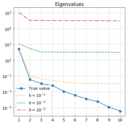
(a) $\sigma=0.01$

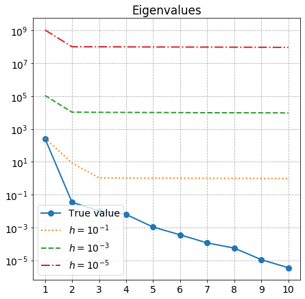
(b) $\sigma=0.1$

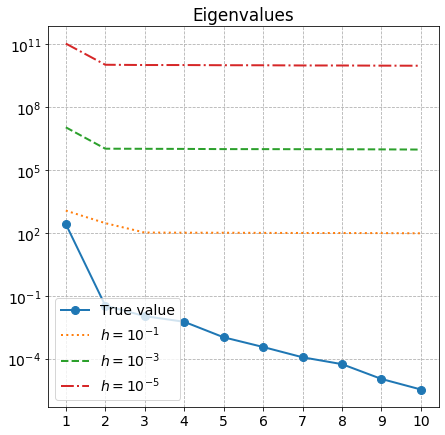
(c) $\sigma=1$

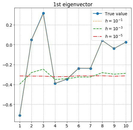
(d) $\sigma=0.01$

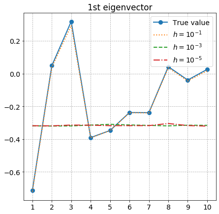
(e) $\sigma=0.1$

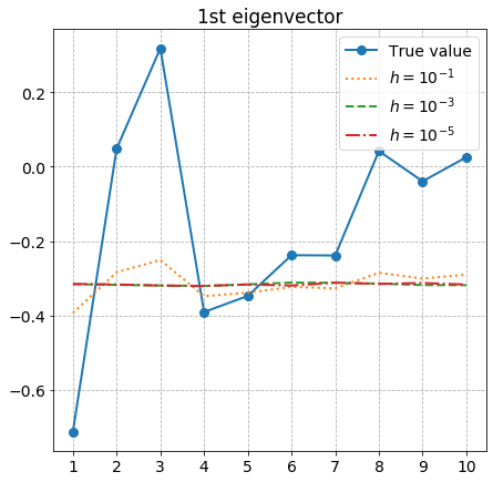
(f) $\sigma=1$

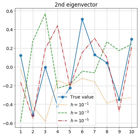
(g) $\sigma=0.01$

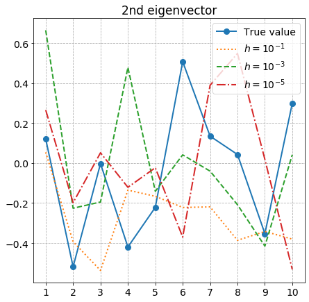
(h) $\sigma=0.1$

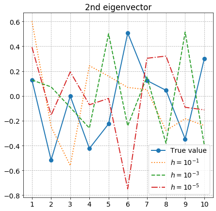
(i) $\sigma=1$

Figure 1: Estimating eigenvalues and eigenvectors for Example 1: AS results.

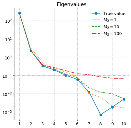
(a) $\sigma=0.01$

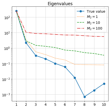
(b) $\sigma=0.1$

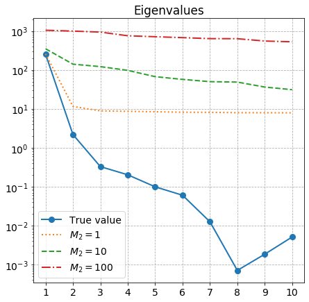
(c) $\sigma=1$

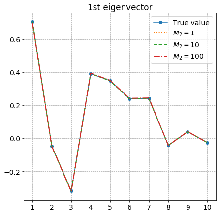
(d) $\sigma=0.01$

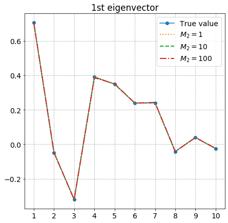
(e) $\sigma=0.1$

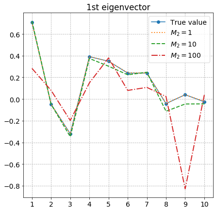
(f) $\sigma=1$

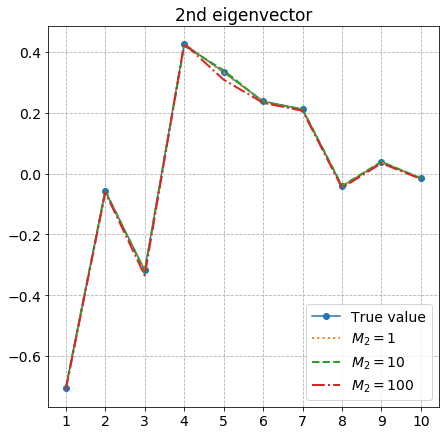
(g) $\sigma=0.01$

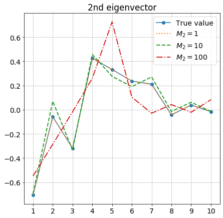
(h) $\sigma=0.1$

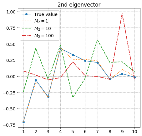
(i) $\sigma=1$

Figure 2: Estimating eigenvalues and eigenvectors for Example 1: GAS results.

In this example we compared the two methods in terms of their accuracy in estimating the eigenvalues and eigenvectors. In the next example we will compare their accuracy when they are used as surrogate models in a computational problem.

5.2 Example 2: Stochastic Computer Models

Stochastic computer models are models where repeated evaluations with the same inputs give different outputs. For the uncertainty quantification and global sensitivity analysis of stochastic computer models, see Fort et al. [13], Hart et al. [16], and Nanty et al. [30].

In this example we consider a stochastic computer model of the form $Y=f(\mathbf{W},\mathbf{V})$. Here $\mathbf{W}$ represents the known uncertainty, and $\mathbf{V}$ represents the model uncertainty. The example is the pricing of an arithmetic Asian call option with discounted payoff

(38) $$g(S_{t_{1}},\ldots,S_{t_{d}})=e^{-rT}\max\left(\frac{1}{d}\sum_{i=1}^{d}S_{t_{i}}-K,0\right),$$

where $S_{t}$ is the price of the underlying at time $t$, $T=t_{d}$ is the expiry, $r$ is the risk-free interest rate, and $K$ is the strike price. We assume the standard Black-Scholes-Merton model for the underlying

$$dS_{t}=rS_{t}dt+\sqrt{V_{t}}S_{t}dW^{1}_{t},$$

where $W^{1}_{t}$ is a standard Brownian motion and $V_{t}$ is the volatility at time $t$. We treat $V_{t}$ as the model uncertainty, represented as

$$V_{t}=H(t,V_{<t},S_{<t},Y_{\leq t}),$$

where $Y_{t}$ is the unknown random process, $V_{<t}$ and $S_{<t}$ are the complete paths of $V_{t}$ and $S_{t}$ before time $t$, and $Y_{\leq t}$ is the complete path of $Y_{t}$ before and including time $t$.

There are several volatility models in the literature, for example, Bollerslev [2], Hull and White [19], Heston [17], Slim [34], and Luo et al. [27]. We assume the true nature of the process $Y_{t}$ is unknown (model uncertainty), but in the numerical results, we will use the Heston model to simulate the volatility process:

(39) $$\begin{split}dV_{t}&=\kappa(\theta-V_{t})dt+\sigma\sqrt{V_{t}}dW^{2}_{t},\\ dW^{1}_{t}dW^{2}_{t}&=\rho dt,\end{split}$$

where $W^{2}_{t}$ is a standard Brownian motion correlated with $W^{1}_{t}$. In other words, $W^{2}_{t}$ is a substitute for the unknown process $Y_{t}$ used in the numerical results. (We assume that the Feller condition $2\kappa\theta>\sigma^{2}$ is satisfied to ensure that $V_{t}$ is strictly positive - see Albrecher et al. [1]).

Under the risk neutral measure, the option price at time zero is given by:

(40) $${\rm E}\,[g(S_{t_{1}},\ldots,S_{t_{d}})]={\rm E}\,[f(W^{1}_{t_{1}},W^{1}_{t_{2}}-W^{1}_{t_{1}},\ldots,W^{1}_{t_{d}}-W^{1}_{t_{d-1}})],$$

where

(41) $$f(z_{1},z_{2},\ldots,z_{d})={\rm E}\,[g(S_{t_{1}},\ldots,S_{t_{d}})|z_{1},z_{2},\ldots,z_{d}],$$

and the conditional expectation is over the probability measure that describes the model uncertainty, the process $Y_{t}$. For a given path $W^{1}_{t_{1}}=z_{1},\ldots,W^{1}_{t_{d}}-W^{1}_{t_{d-1}}=z_{d}$, the conditional expectation is estimated, in the numerical results, by simulating ten paths for the volatility process $V_{t}$ using the Heston model. This approach of conditioning on the distribution for model uncertainty to turn the stochastic computer code to a deterministic one is used in the literature, for example, by Mazo [29], and Iooss and Ribatet [20].

We apply the AS and GAS methods to the function $f(z_{1},z_{2},\dots,z_{d})$. Each method yields a different vector $\hat{\boldsymbol{w}}_{1}$ of length $d_{1}$, the vector that contains the important directions of the function. We then construct surrogate models that are functions of $\hat{\boldsymbol{w}}_{1}$ for each method. The option price is estimated by computing the expected value of the surrogate model corresponding to AS and GAS methods.

In our numerical results, we choose $T=1,d=10,S_{0}=K=100,V_{0}=0.04,r=0.03,\kappa=2,\theta=0.04,\sigma=0.09$, and $\rho=0.9$. For the AS method, we use a Monte Carlo sample size of $10,000$ to estimate the expectations in the matrix $C$. For the GAS method, we set $M_{1}=10,000$ and $M_{2}=1$ (see Eqn. (12)).

Table 1 displays the estimated cumulative eigenvalues $\frac{\sum_{k=1}^{i}\hat{\lambda}_{j}}{\sum_{k=1}^{d}\hat{\lambda}_{j}}$, where $\hat{\lambda}_{j}$’s are written in decreasing order. Figure 3 plots the coefficients of the first eigenvector of $\hat{\boldsymbol{C}}$ for each method. We observe that the cumulative eigenvalues of the GAS method approaches to one faster than the AS method (Table 1). The first eigenvectors of AS and GAS (Fig. 3) are not close to each other at all, suggesting that the resulting subspaces will be different.

	1	2	3	4	5	6	7	8	9	10
AS	0.556	0.612	0.666	0.717	0.767	0.816	0.863	0.910	0.955	1.
GAS	0.921	0.949	0.968	0.981	0.990	0.995	0.998	0.999	1.	1.

Table 1: Cumulative eigenvalues for Example 2

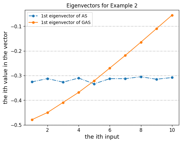
Figure 3: Coefficients of the first eigenvector of $\hat{\boldsymbol{C}}$ for Example 2

Based on the largest gap between estimated eigenvalues, we choose $d_{1}=1$ for both methods. We choose $N=10,000$ and $N_{1}=1$ to construct the surrogate models in Algorithm 1. To estimate the integral ${\rm E}\,[f(\boldsymbol{z})],\boldsymbol{z}=(z_{1},\ldots,z_{d})$, we consider the following four estimators:

• Monte Carlo (MC): $\frac{1}{N}\sum_{i=1}^{N}f(\boldsymbol{z}^{(i)})$, $\boldsymbol{z}^{(i)}\sim\mathcal{N}(\boldsymbol{0},\boldsymbol{I_{d}}),i=1,\ldots,N$.

• Polynomial chaos expansion (PCE): $\hat{k}_{0}$, where $\hat{k}_{0}$ is obtained from the estimated PCE constructed from the data $(\boldsymbol{z}^{(i)},f(\boldsymbol{z}^{(i)})),\boldsymbol{z}^{(i)}\sim\mathcal{N}(\boldsymbol{0},\boldsymbol{I_{d}}),i=1,\ldots,N$ (see Eqns. (17) and (18)).

• AS_PCE: $\hat{k}_{0}$, where $\hat{k}_{0}$ is obtained from the estimated PCE constructed from the data $(\boldsymbol{z}^{(i)},\hat{G}_{mc}(\boldsymbol{z}^{(i)})),\boldsymbol{z}^{(i)}\sim\mathcal{N}(\boldsymbol{0},\boldsymbol{I_{d_{1}}}),i=1,\ldots,N$. Here $\hat{G}_{mc}(\boldsymbol{z}^{(i)})$ is computed as in Constantine [4].

• GAS_PCE: $\hat{k}_{0}$, where $\hat{k}_{0}$ is obtained from the estimated PCE constructed from the data $(\boldsymbol{z}^{(i)},\hat{G}_{mc}(\boldsymbol{z}^{(i)})),\boldsymbol{z}^{(i)}\sim\mathcal{N}(\boldsymbol{0},\boldsymbol{I_{d_{1}}}),i=1,\ldots,N$. Here $\hat{G}_{mc}(\boldsymbol{z}^{(i)})$ is computed using Algorithm 1.

For each estimator, we repeat the numerical approximation $40$ times, independently, and obtain estimates $E_{1},\ldots,E_{40}$. We then compute the mean square error (MSE) of the estimates:

(42) $$MSE=\frac{1}{40}\sum_{i=1}^{40}(E_{i}-E_{true})^{2},$$

where $E_{true}$ is the result of the Monte Carlo estimator using a sample size of $N=10^{6}$.

We define the efficiency of each method as $1/(Time\times MSE)$, where time is the computing time (seconds) to generate the 40 estimates (including the computation of the matrices $\hat{\boldsymbol{C}}$, their singular value decomposition, and construction of the surrogate models). Higher efficiency means a better method. Figure 4 plots the logarithm of MSE and Efficiency of the methods, as a function of the truncation level $p$ for the PCE based methods. The MSE of GAS_PCE and PCE are similar, and they are significantly smaller than that of AS_PCE. In terms of efficiency, the best method is GAS_PCE.

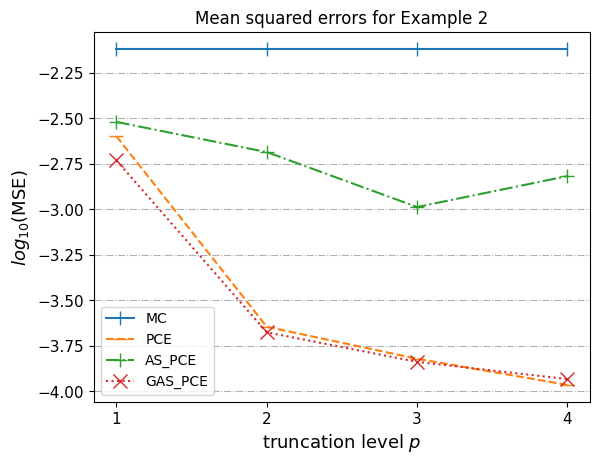
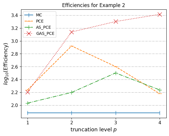
Figure 4: MSEs and efficiencies for Example 2

Figure 4 compares the methods for a particular choice of parameters $\sigma$ and $\rho$ (see Eqn. (39)) that determine the randomness due to model uncertainty. To compare the methods for a variety of choices for $\sigma$ and $\rho$, we proceed as follows. We select several values for $\sigma$ and $\rho$ while keeping the other parameters as constants. We choose $T=1,d=10,S_{0}=K=100,V_{0}=0.025,r=0.03,\kappa=3,\theta=0.025,\sigma=0.01,0.05,0.1,0.15,0.2,\rho=-0.99,-0.9,-0.5,0,0.5,0.9,0.99$. These parameter values are based on Table 5 of Escobar and Gschnaidtner [12]. For each set of parameters, we compute the PCE using a truncation level of $p=3$ for all the PCE based methods (PCE, AS_PCE, GAS_PCE). We then calculate the ratio of the MSE of GAS_PCE to the MSE of AS_PCE, and the ratio of the efficiency of GAS_PCE to the efficiency of AS_PCE.

Figures 5-7 are heatmaps displaying the ratios of MSE and efficiency for several choices for $M_{1},M_{2}$ for the GAS method: $M_{1}=10,000,M_{2}=1$; $M_{1}=1,000,M_{2}=10$; and $M_{1}=100,M_{2}=100$. For the AS method the Monte Carlo sample size is $10,000$. In the figures the MSE and efficiency ratios that are less than one are displayed in blue, and ratios that are larger than one in red. Therefore blue in the MSE plots indicates the GAS method has lower error than AS, and red in the efficiency plots indicates the GAS method has better efficiency than AS, for the corresponding parameter choices. We observe that for every choice of parameters, and every choice of $M_{2}$, the GAS method has better accuracy (smaller MSE) and better efficiency than the AS method.

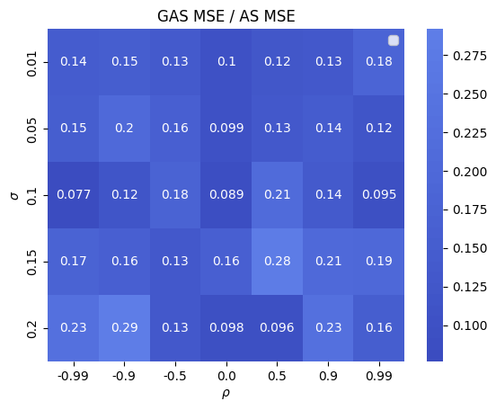
Figure 5: MSE and efficiency ratios for $M_{2}=1$

‘

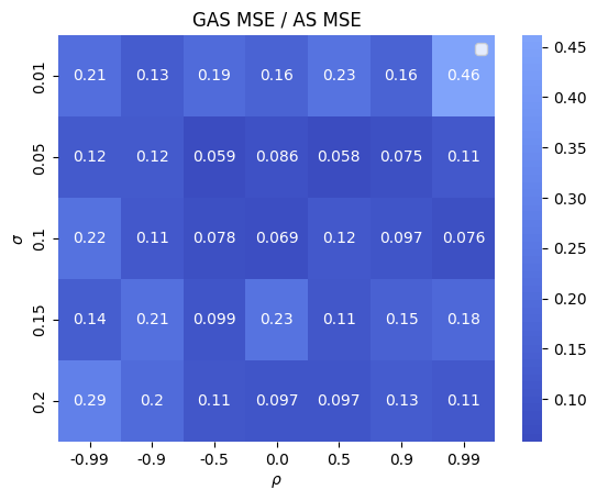
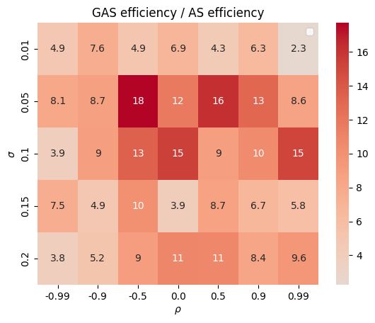
Figure 6: MSE and efficiency ratios for $M_{2}=10$

‘

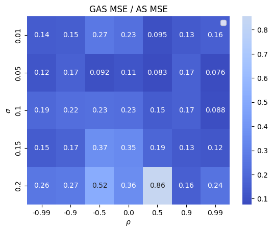
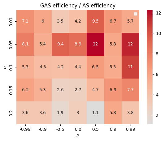
Figure 7: MSE and efficiency ratios for $M_{2}=100$

‘

5.3 Example 3: Discontinuous Functions

The AS method requires the existence of the partial derivatives of the function: the entries of the matrix $\boldsymbol{C}$ are expected values of partial derivatives. The GAS method does not require the existence of partial derivatives, since the entries of the matrix $\boldsymbol{C}$ for GAS are expected values of finite-differences. However, the error analysis of the GAS method assumes the existence of partial derivatives. In the previous example we considered a function that was not differentiable everywhere. In this example we consider a discontinuous function to further examine the effectiveness of the methods when assumptions used in their theoretical analysis are violated.

Hoyt and Owen [18] consider the mean dimension of ridge functions, including the cases when the ridge functions are discontinuous. We consider the following example from their paper

(43) $$f(\boldsymbol{z})=\boldsymbol{1}\{\theta^{T}\boldsymbol{z}>0\},\boldsymbol{z}\in\mathbb{R}^{d},$$

where $\boldsymbol{1}\{\theta^{T}\boldsymbol{z}>0\}$ equals 1 if $\theta^{T}\boldsymbol{z}>0$ and zero otherwise, and we assume the domain of $f$ is equipped with the CDF of a $d$-dimensional standard normal random variable.

We consider two cases: $d=10$ and $d=20$. In each case, we choose $\theta$ by randomly generating a $d$-dimensional vector from the multivariate standard normal distribution. We then estimate the first eigenvector of $\hat{\boldsymbol{C}}$ for the AS and GAS methods. For the AS method, we take the Monte Carlo sample size to be $10,000$, and $h=10^{-1},10^{-3}$ and $10^{-5}$. For the GAS method, we take $M_{2}=1,10,100$ while maintaining $M_{1}M_{2}=10,000$. Figure 8 plots the first estimated eigenvector for each method, together with the vector $\theta$, for $d=10$ and $d=20$.

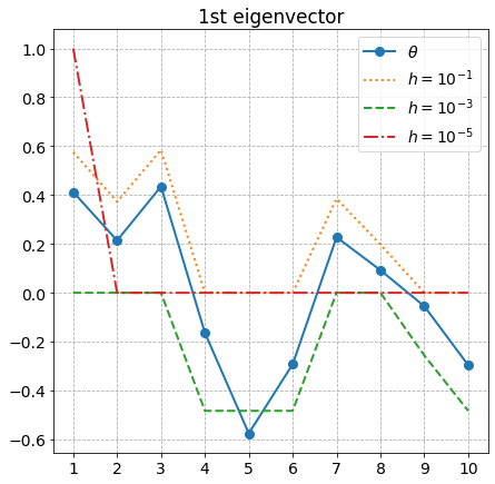
(a) AS method, $d=10$

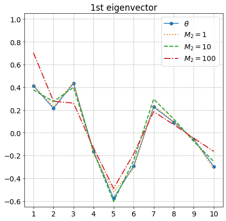
(b) GAS method, $d=10$

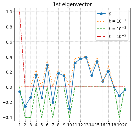
(c) AS method, $d=20$

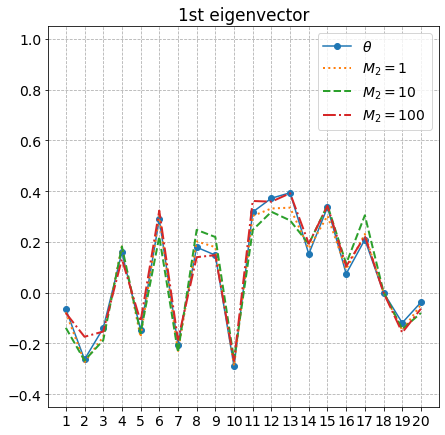
(d) GAS method, $d=20$

Figure 8: Coefficients of the first eigenvector of $\hat{\boldsymbol{C}}$ for Example 3

The accuracy of the GAS method, compared to the accuracy of AS, is significantly better for all choices for $M_{2}$. The best GAS estimation happens when $M_{2}=1$. The AS method gives somewhat meaningful estimates only when $h=10^{-1}$ and $d=20$.

5.4 Example 4: An Ebola Model

In this example we consider the global sensitivity analysis of a modified SEIR model for the spread of Ebola introduced in Diaz et al. [11]. The model is a system of seven differential equations which describe the dynamics of disease within a population. The output we are interested in is the basic reproduction number $R_{0}$, and Diaz et al. [11] shows that $R_{0}$ is

(44) $$R_{0}=\frac{\beta_{1}+\frac{\beta_{2}\rho_{1}\gamma_{1}}{\omega}+\frac{\beta_{3}}{\gamma_{2}}\psi}{\gamma_{1}+\psi},$$

where $\beta_{1},\beta_{2},\beta_{3},\rho_{1},\gamma_{1},\gamma_{2},\omega$ and $\psi$ are the model parameters. Table 2, which is from [11], displays the distributions of the parameters, obtained using data from the country Liberia.

Parameter	$\beta_{1}$	$\beta_{2}$	$\beta_{3}$	$\rho_{1}$
Liberia	$U(.1,.4)$	$U(.1,.4)$	$U(.05,.2)$	$U(.41,1)$
Parameter	$\gamma_{1}$	$\gamma_{2}$	$\omega$	$\psi$
Liberia	$U(.0276,.1702)$	$U(.081,.21)$	$U(.25,.5)$	$U(.0833,.7)$

Table 2: Parameter distributions in Ebola model

The problem can be rewritten as $f(\boldsymbol{z})=R_{0}$, where $z_{i}\sim U(0,1),i=1,\dots,8$. We apply the AS and GAS methods to $f$ using a Monte Carlo sample size of $10,000$ and $h=0.001$ for AS, and $M_{1}=1000$ and $M_{2}=10$ for GAS. Tables 3 displays the cumulative eigenvalues and the first eigenvector of $\hat{\boldsymbol{C}}$ for AS and GAS methods.

Cumulative eigenvalues	1	2	3	4	5	6	7	8
AS	0.769	0.967	0.985	0.995	0.999	1.	1.	1.
GAS	0.797	0.929	0.969	0.988	0.996	0.999	1.	1.
$1$st eigenvector	1	2	3	4	5	6	7	8
AS	0.385	0.062	0.340	0.043	-0.252	-0.298	-0.038	-0.759
GAS	0.464	0.077	0.490	0.055	-0.251	-0.389	-0.046	-0.565

Table 3: Comparison of results for Liberia

Figures 9 and 10 plot the eigenvalues, eigenvectors, and sufficient summary plots for the first active variable $\hat{\boldsymbol{U}}^{(1)}\boldsymbol{z}$, and the first and second active variable $\hat{\boldsymbol{U}}^{(2)}\boldsymbol{z}$ together, for the AS and GAS methods, using the data from Liberia only (data from Sierra Leone give similar conclusions). Here $\hat{\boldsymbol{U}}^{(1)}$ and $\hat{\boldsymbol{U}}^{(2)}$ are the first two eigenvectors, that is the first two columns of $\hat{\boldsymbol{U}}$. The sufficient summary plot for the first active variable is obtained by plotting the output $R_{0}$ for a sample of $2,000$ randomly generated inputs $\hat{\boldsymbol{U}}^{(1)}\boldsymbol{z}^{(i)},i=1,\ldots,2000.$ The sufficient summary plot for the first and second active variables is also based on 2,000 random samples for each variable. We observe that the first eigenvector for AS and GAS methods are very similar, as well as their sufficient summary plots We conclude both methods give very similar results in this example.

(a) Eigenvalues

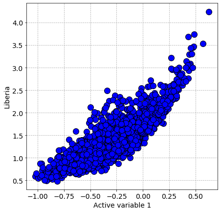
(b) Sufficient summary plot 1

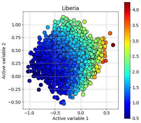
(c) Sufficient summary plot 2

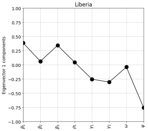
(d) 1st eigenvector

Figure 9: AS results for Ebola model (Liberia)

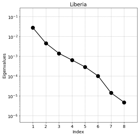
(a) Eigenvalues

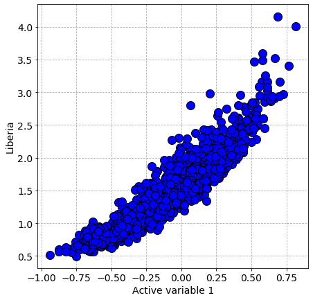
(b) Sufficient summary plot 1

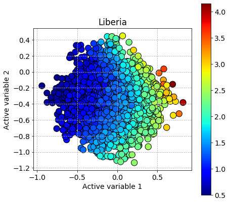
(c) Sufficient summary plot 2

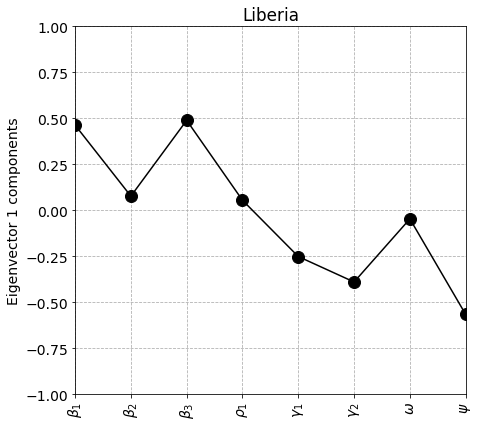
(d) 1st eigenvector

Figure 10: GAS results for Ebola model (Liberia)

6 Conclusions

The global active subspace method uses a global measure for change in function values, the expected value of first-order finite differences, in finding the important directions along which the function changes the most. We have established the error analysis of the method and presented numerical results comparing the method with the active subspace method. Like the active subspace method, the effectiveness of the global active subspace method depends on how fast the eigenvalues of $\boldsymbol{C}$ decay. In the numerical results we have observed that the method is superior to the active subspace method when it is difficult to estimate the gradients, such as in the presence of noise. The method can be applied to non-differentiable functions, although its error analysis requires differentiability. We also observed that the method gave comparable results to the active subspace method when the estimation of the gradient was not problematic, like in the Ebola model. We believe the global active subspace method is a promising dimension reduction method for complex models.

References

- [1] H. Albrecher, P. Mayer, W. Schoutens, and J. Tistaert, The little Heston trap, Wilmott Magazine, (2007), pp. 83–92.
- [2] T. Bollerslev, Generalized autoregressive conditional heteroskedasticity, Journal of Econometrics, 31 (1986), pp. 307–327.
- [3] K. D. Coleman, A. Lewis, R. C. Smith, B. Williams, M. Morris, and B. Khuwaileh, Gradient-free construction of active subspaces for dimension reduction in complex models with applications to neutronics, SIAM/ASA Journal on Uncertainty Quantification, 7 (2019), pp. 117–142.
- [4] P. G. Constantine, Active subspaces: Emerging ideas for dimension reduction in parameter studies, SIAM, 2015.
- [5] P. G. Constantine, E. Dow, and Q. Wang, Active subspace methods in theory and practice: applications to kriging surfaces, SIAM Journal on Scientific Computing, 36 (2014), pp. A1500–A1524.
- [6] P. G. Constantine, A. Eftekhari, and M. B. Wakin, Computing active subspaces efficiently with gradient sketching, in 2015 IEEE 6th International Workshop on Computational Advances in Multi-Sensor Adaptive Processing (CAMSAP), IEEE, 2015, pp. 353–356.
- [7] P. G. Constantine, M. Emory, J. Larsson, and G. Iaccarino, Exploiting active subspaces to quantify uncertainty in the numerical simulation of the Hyshot II scramjet, Journal of Computational Physics, 302 (2015), pp. 1–20.
- [8] P. G. CONSTANTINE and D. F. GLEICH, Computing active subspaces with Monte Carlo, arXiv preprint arXiv:1408.0545, (2014).
- [9] C. Cui, K. Zhang, T. Daulbaev, J. Gusak, I. Oseledets, and Z. Zhang, Active subspace of neural networks: Structural analysis and universal attacks, SIAM Journal on Mathematics of Data Science, 2 (2020), pp. 1096–1122.
- [10] N. Demo, M. Tezzele, and G. Rozza, A supervised learning approach involving active subspaces for an efficient genetic algorithm in high-dimensional optimization problems, SIAM Journal on Scientific Computing, 43 (2021), pp. B831–B853.
- [11] P. Diaz, P. Constantine, K. Kalmbach, E. Jones, and S. Pankavich, A modified SEIR model for the spread of Ebola in Western Africa and metrics for resource allocation, Applied Mathematics and Computation, 324 (2018), pp. 141–155.
- [12] M. Escobar and C. Gschnaidtner, Parameters recovery via calibration in the Heston model: A comprehensive review, Wilmott, 86 (2016), pp. 60–81.
- [13] J.-C. Fort, T. Klein, and A. Lagnoux, Global sensitivity analysis and Wasserstein spaces, SIAM/ASA Journal on Uncertainty Quantification, 9 (2021), pp. 880–921.
- [14] G. H. Golub and C. F. Van Loan, Matrix computations, JHU press, 2013.
- [15] J. Hampton and A. Doostan, Coherence motivated sampling and convergence analysis of least squares polynomial chaos regression, Computer Methods in Applied Mechanics and Engineering, 290 (2015), pp. 73–97.
- [16] J. L. Hart, A. Alexanderian, and P. A. Gremaud, Efficient computation of Sobol’ indices for stochastic models, SIAM Journal on Scientific Computing, 39 (2017), pp. A1514–A1530.
- [17] S. L. Heston, A closed-form solution for options with stochastic volatility with applications to bond and currency options, The Review of Financial Studies, 6 (1993), pp. 327–343.
- [18] C. R. Hoyt and A. B. Owen, Mean dimension of ridge functions, SIAM Journal on Numerical Analysis, 58 (2020), pp. 1195–1216.
- [19] J. Hull and A. White, The pricing of options on assets with stochastic volatilities, The Journal of Finance, 42 (1987), pp. 281–300.
- [20] B. Iooss and M. Ribatet, Global sensitivity analysis of computer models with functional inputs, Reliability Engineering & System Safety, 94 (2009), pp. 1194–1204.
- [21] J. L. Jefferson, J. M. Gilbert, P. G. Constantine, and R. M. Maxwell, Active subspaces for sensitivity analysis and dimension reduction of an integrated hydrologic model, Computers & Geosciences, 83 (2015), pp. 127–138.
- [22] F. Kubler, S. Scheidegger, et al., Self-justified equilibria: Existence and computation, in 2018 Meeting Papers, no. 694, Society for Economic Dynamics, 2018.
- [23] A. Lewis, R. Smith, and B. Williams, Gradient free active subspace construction using Morris screening elementary effects, Computers & Mathematics with Applications, 72 (2016), pp. 1603–1615.
- [24] J. Li, J. Cai, and K. Qu, Surrogate-based aerodynamic shape optimization with the active subspace method, Structural and Multidisciplinary Optimization, 59 (2019), pp. 403–419.
- [25] S. Liu and A. B. Owen, Preintegration via active subspace, SIAM Journal on Numerical Analysis, 61 (2023), pp. 495–514.
- [26] T. W. Lukaczyk, P. Constantine, F. Palacios, and J. J. Alonso, Active subspaces for shape optimization, in 10th AIAA Multidisciplinary Design Optimization Conference, 2014, p. 1171.
- [27] R. Luo, W. Zhang, X. Xu, and J. Wang, A neural stochastic volatility model, in Proceedings of the AAAI Conference on Artificial Intelligence, vol. 32, 2018.
- [28] H. Ma, E.-P. Li, A. C. Cangellaris, and X. Chen, Support vector regression-based active subspace (SVR-AS) modeling of high-speed links for fast and accurate sensitivity analysis, IEEE Access, 8 (2020), pp. 74339–74348.
- [29] G. Mazo, An optimal tradeoff between explorations and repetitions in global sensitivity analysis for stochastic computer models, Preprint hal-02113448, (2019).
- [30] S. Nanty, C. Helbert, A. Marrel, N. Pérot, and C. Prieur, Sampling, metamodelling and sensitivity analysis of numerical simulators with functional stochastic inputs, HAL, 2016 (2016).
- [31] N. Navaneeth and S. Chakraborty, Surrogate assisted active subspace and active subspace assisted surrogate—a new paradigm for high dimensional structural reliability analysis, Computer Methods in Applied Mechanics and Engineering, 389 (2022), p. 114374.
- [32] A. Saltelli, P. Annoni, I. Azzini, F. Campolongo, M. Ratto, and S. Tarantola, Variance based sensitivity analysis of model output. Design and estimator for the total sensitivity index, Computer Physics Communications, 181 (2010), pp. 259–270.
- [33] A. Saltelli, M. Ratto, T. Andres, F. Campolongo, J. Cariboni, D. Gatelli, M. Saisana, and S. Tarantola, Global sensitivity analysis: the primer, John Wiley & Sons, 2008.
- [34] C. Slim, Forecasting the volatility of stock index returns: A stochastic neural network approach, in International Conference on Computational Science and Its Applications, Springer, 2004, pp. 935–944.
- [35] I. Sobol, On the distribution of points in a cube and the approximate evaluation of integrals, USSR Computational Mathematics and Mathematical Physics, 7 (1967), pp. 86–112.
- [36] I. M. Sobol’, Global sensitivity indices for nonlinear mathematical models and their Monte Carlo estimates, Mathematics and Computers in Simulation, 55 (2001), pp. 271–280.
- [37] J. A. Tropp, User-friendly tail bounds for sums of random matrices, Foundations of Computational Mathematics, 12 (2012), pp. 389–434.
- [38] N. Wycoff, M. Binois, and S. M. Wild, Sequential learning of active subspaces, Journal of Computational and Graphical Statistics, 30 (2021), pp. 1224–1237.
- [39] D. Xiu and G. E. Karniadakis, The Wiener–Askey polynomial chaos for stochastic differential equations, SIAM Journal on Scientific Computing, 24 (2002), pp. 619–644.
- [40] H. Yan, C. Hao, J. Zhang, W. A. Illman, G. Lin, and L. Zeng, Accelerating groundwater data assimilation with a gradient-free active subspace method, Water Resources Research, 57 (2021), p. e2021WR029610.
- [41] T. Zhou and Y. Peng, Active learning and active subspace enhancement for PDEM-based high-dimensional reliability analysis, Structural Safety, 88 (2021), p. 102026.