Breakup of quantum liquid filaments into droplets

Abstract

We have investigated how the Rayleigh-Plateau instability of a filament made of a ⁴¹K-⁸⁷Rb self-bound mixture may lead to an array of identical quantum droplets, with typical breaking times which are shorter than the lifetime of the mixture. If the filament is laterally confined –as it happens in a toroidal trap– and atoms of one species are in excess with respect to the optimal, equilibrium ratio, the droplets are immersed into a superfluid background made by the excess species which provides global phase coherence to the system, suggesting that the droplets array in the unbalanced system may display supersolid character. This possibility has been investigated by computing the non-classical translational inertia coefficient. The filament may be a reasonable representation of a self-bound mixture subject to toroidal confinement when the bigger circle radius of the torus is much larger than the filament radius.

I Introduction

A new quantum state of matter has been predicted petrov2015quantum to occur in ultracold atomic gases composed of binary mixtures of Bose atoms where the competition between the inter-species attractive interactions and quantum fluctuations, which produce a repulsive interaction, may lead to the formation of self-bound liquid droplets with ultralow densities about eight orders of magnitude lower than those, e.g., of the prototypical quantum fluid, namely liquid Helium. Such novel quantum state was first observed experimentally in dipolar Bose gases Pfau ; Ferlaino , by exploiting the competition between contact repulsion and dipole-dipole attraction, and later in ultracold binary mixtures of Bose atoms cabrera2018quantum ; semeghini2018self ; derrico2019observation ; NaRb2021 .

Several binary Bose mixtures which may convert into quantum liquids have been investigated so far. At variance with the largely studied short-lived homonuclear mixture of ³⁹K atoms in two different hyperfine states, the heteronuclear ⁴¹K-⁸⁷Rb mixture studied in Ref. derrico2019observation, , which forms a quantum liquid state when the ⁴¹K-⁸⁷Rb scattering length $a_{12}$ becomes lower than the critical value $a_{12}=-73.6\,a_{0}$ derrico2019observation ($a_{0}$ being the Bohr radius), is rather long-lived with lifetimes of the order of several tens of milliseconds, i.e., more than an order of magnitude larger than those characterizing the ³⁹K mixtures semeghini2018self . This opens the possibility of studying phenomena whose dynamical development requires time periods in the millisecond range. One such phenomenon is the dynamical instability of quantum liquid filaments leading to quantum drops formation, which is the subject of this work.

Liquid filaments (i.e. threads of liquid with the approximate shape of straight, long cylinders) –and their dynamical instabilities– are thoroughly studied subjects in classical fluids dynamics both because of the underlying fundamental physical properties and their potential applications. Experiments in this field, mainly concentrated on viscous fluids, are interpreted using theoretical approaches based on the solution of the Navier-Stokes equation subject to appropriate boundary conditions. For an extended review on the subject see e.g. Ref. Egg08, and references therein.

The stability of a macroscopic liquid filament, modelled with an infinitely extended cylinder of radius $R$, was studied by Plateau,Pla57 showing that it exists in an unstable equilibrium, and any perturbation with wavelength $\lambda$ greater than $2\pi R$ triggers an instability where the surface tension breaks the cylinder into droplets. Lord Rayleigh later showedRay79 that for an inviscid and incompressible liquid the fastest growing mode occurs when the wavelength of the axial undulation that leads to the fragmentation of the liquid filament into droplets is equal to $\lambda_{c}=9.01\,R$ or, equivalently, $kR=0.697$, where $k=2\pi/\lambda_{c}$ (Rayleigh-Plateau instability). When the filament breaks up, one or more small satellite drops -resulting from the necks breaking- may form between the larger droplets.

Rayleigh-type instabilities are not limited to classical fluid only, but may affect also quantum fluids. The dynamics of contraction and breaking of zero temperature superfluid ⁴He liquid thin filaments in vacuum, triggered by the above kind of instabilities, has recently been addressedAnc23 using a ⁴He Density Functional Theory approach which accurately describes superfluid ⁴He at zero temperatureAnc17 .

We investigate here the instability of thin filaments made of another superfluid system, namely a quantum liquid made of an ultracold bosonic ⁴¹K-⁸⁷Rb mixture. We notice that the instability of a two-component Bose-Einstein condensate has been investigated saito in the repulsive (immiscible) regime, where a cylindrical condensate made of one species surrounded by the other component was found to undergo breakup into gaseous bubbles.

We consider here a linear, thin filament with periodic boundary conditions imposed at its ends. One can consider such geometry as a limiting case of a mixture subject to a toroidal confinement when the bigger circle radius of the torus is much larger than the filament radius.

To study the instability of quantum liquid filaments we will use two different approaches. One is the widely known Mean-Field+Lee-Huang-Yang (MF-LHY) approximation which provides a reliable description of the binary mixture in the quantum liquid regime through the solution in three dimensions of two coupled non-linear Gross-Pitaevskii (GP) equations, and which applies to arbitrary concentrations of the two species. Since in the quantum liquid state of the ⁴¹K-⁸⁷Rb uniform mixture the equilibrium densities of the two components are expected to have a fixed ratio, the system can be effectively described by one single wave function satisfying an effective GP equationPol21 . Inspired in the work carried out in Ref. Sal02, for one-component BEC gases, in a second approach we will use a variational formalism suited to the geometry we are implementing in the present work. This allows one to reduce the coupled three-dimensional (3D) GP equations to one effective one-dimensional (1D) GP equation plus an algebraic equation. We verify the feasibility of this simplified approach by comparing the filament properties it yields with the ones obtained by solving the 3D coupled GP equations. Either approach will disclose the time scale for filament breakup and the appearance of quantum droplets as a result of its fragmentation.

In the second part of this work we will address an interesting aspect arising when one of the species is in excess with respect to the optimal density ratio and the droplets resulting from filament breakup are immersed in a superfluid background made by the species in excess, which provides global phase coherence to the system and may lead to supersolid behavior. Such possibility is investigated by computing the non-classical translational inertia associated to this system.

This work is organized as follows. In Sec. II we review the theoretical approach used to describe the binary mixture in the quantum liquid regime, which is based on the MF-LHY approximation, and also introduce a simpler yet accurate variational approach based on a 1D effective equation introduced some time ago to describe single-component Bose Einstein condensates subject to tight radial harmonic confinement Sal02 . Such approach is extended here to the quantum liquid mixture case and is used to address the dynamical instability of quantum liquid filaments leading to quantum droplets formation. The results are presented in Sec. III, and a summary is given in Sec. IV.

II Method

The Gross-Pitaevskii energy functional for a Bose-Bose mixture, including the Lee-Huang-Yang correction accounting for quantum fluctuations beyond mean-field reads petrov2015quantum ; ancilotto2018self

$$E=\sum_{i=1}^{2}\int d{\bf r}\,\left[{\hbar^{2}\over 2m_{i}}|\nabla\psi_{i}({\bf r})|^{2}+V_{i}({\bf r})\rho_{i}({\bf r})\right]\,+\frac{1}{2}\sum_{i,j=1}^{2}g_{ij}\int d{\bf r}\,\rho_{i}({\bf r})\rho_{j}({\bf r})\,+\int d{\bf r}\,{\cal E}_{\rm LHY}(\rho_{1}({\bf r}),\rho_{2}({\bf r}))\,,$$ (1)

where $V_{i}({\bf r})$ and $\rho_{i}({\bf r})=|\psi_{i}({\bf r})|^{2}$ represent the external potential and the number density of each component ($i=1$ for ⁴¹K, $i=2$ for ⁸⁷Rb), respectively. The coupling constants are $g_{11}=4\pi a_{11}\hbar^{2}/m_{1}$, $g_{22}=4\pi a_{22}\hbar^{2}/m_{2}$, and $g_{12}=g_{21}=2\pi a_{12}\hbar^{2}/m_{r}$, where $m_{r}=m_{1}m_{2}/(m_{1}+m_{2})$ is the reduced mass. The number densities $\rho_{1},\,\rho_{2}$ are normalized such that $\int_{V}\rho_{1}({\bf r})\,{\rm d}{\bf r}=N_{1}$ and $\int_{V}\rho_{2}({\bf r})\,{\rm d}{\bf r}=N_{2}$. The intra-species $s$-wave scattering lengths $a_{11}$ and $a_{22}$ are both positive, while the inter-species one, $a_{12}$, is negative. The scattering parameters describing the intraspecies repulsion are fixed and their values are equal to $a_{11}=65\,a_{0}$ derrico2007feshbach and $a_{22}=100.4\,a_{0}$ marte . The heteronuclear scattering length $a_{12}$ can be tuned by means of Feshbach resonances. The onset of the mean-field collapse regime leading to the quantum liquid state corresponds to $g_{12}+\sqrt{g_{11}g_{22}}=0$, which occurs at $a_{12}=-73.6\,a_{0}$ derrico2019observation .

The LHY correction is petrov2015quantum ; ancilotto2018self

$${\cal E}_{\rm LHY} ={8\over 15\pi^{2}}\left(\frac{m_{1}}{\hbar^{2}}\right)^{3/2}\!\!\!\!\!\!(g_{11}\rho_{1})^{5/2}f\left(\frac{m_{2}}{m_{1}},\frac{g_{12}^{2}}{g_{11}g_{22}},\frac{g_{22}\,\rho_{2}}{g_{11}\,\rho_{1}}\right)$$

$$\equiv\mathcal{C}(g_{11}\rho_{1})^{5/2}f(z,u,x).$$ (2)

Here, $f(z,u,x)>0$ is a dimensionless function whose explicit expression for an heteronuclear mixture can be found in Ref. ancilotto2018self, . Following Ref. petrov2015quantum, , we consider this function at the mean-field collapse $u=1$, i.e., ${\cal E}_{\rm LHY}=\mathcal{C}(g_{11}\rho_{1})^{5/2}f(z,1,x)$. We note that the actual expression for $f$ can be fitted very accurately with the same functional form of the homonuclear ($m_{1}=m_{2}$) caseMinardi

$$f\left(z,1,x\right)=\left(1+z^{\alpha_{1}}x\right)^{\beta_{1}}\,,$$ (3)

where $\alpha_{1}$ and $\beta_{1}$ are fitting parameters. For the ⁴¹K-⁸⁷Rb mixture ($z=87/41$) one has Minardi $\alpha_{1}=0.586$ and $\beta_{1}=2.506$. We will use the form in Eq. (3) for our calculations.

II.1 3D equations

Minimization of the action associated to Eq. (1) leads to the following Euler-Lagrange equations (generalized GP equations)

$$i\hbar{\partial\psi_{i}\over\partial t}=\left[-{\hbar^{2}\over 2m_{i}}\nabla^{2}+V_{i}+\mu_{i}(\rho_{1},\rho_{2})\right]\psi_{i}\,,$$ (4)

where

$$\mu_{i}=g_{ii}\rho_{i}+g_{ij}\rho_{j}+\frac{\partial{\cal E}_{\rm LHY}}{\partial\rho_{i}}\quad\,(j\neq i)$$ (5)

and

$$\frac{\partial{\cal E}_{\rm LHY}}{\partial\rho_{1}} =\mathcal{C}\,g_{11}(g_{11}\rho_{1})^{3/2}\left({5\over 2}f-x{\partial f\over\partial x}\right)$$ (6)

$$\frac{\partial{\cal E}_{\rm LHY}}{\partial\rho_{2}} =\mathcal{C}\,g_{22}(g_{11}\rho_{1})^{3/2}{\partial f\over\partial x}\,,$$ (7)

where $\mathcal{C}$ is defined in Eq. (2).

The numerical solutions of Eqs. (4) provide the time-evolution of a ⁴¹K-⁸⁷Rb mixture with arbitrary compositions $N_{1},N_{2}$ in three-dimensions. In the following, we will refer to this solution as the 3D model to distinguish it from a simpler, computationally faster 1D model approach which we will describe next.

II.2 Effective 1D equation

The mixture of the two bosonic species in the homogeneous phase is stable against fluctuations in the concentration $N_{1}/N_{2}$ if petrov2015quantum

$$\dfrac{\rho_{1}}{\rho_{2}}=\sqrt{\dfrac{g_{22}}{g_{11}}}\ .$$ (8)

For the ⁴¹K-⁸⁷Rb system investigated in the present work, $\rho_{1}/\rho_{2}=0.853$. As pointed out in Refs. petrov2015quantum, ; ancilotto2018self, ; staudinger2018self, , it is safe to assume that this optimal composition is realized everywhere in the system. Therefore, the energy functional Eq. (1) becomes effectively single-component and can be expressed in terms of the density $\rho_{1}$ alone as $E=\int\mathcal{E}(\mathbf{r})$ d$\mathbf{r}$, where

$$\mathcal{E}=\alpha\frac{(\nabla\rho_{1})^{2}}{\rho_{1}}+\beta\rho_{1}^{2}+\gamma\rho_{1}^{5/2}$$ (9)

with

$$\alpha=\frac{1}{4}\left(\frac{\hbar^{2}}{2m_{1}}+\frac{\hbar^{2}}{2m_{2}}\sqrt{\frac{g_{11}}{g_{22}}}\right)$$ (10)

$$\beta=g_{11}+g_{12}\sqrt{\frac{g_{11}}{g_{22}}}$$ (11)

$$\gamma={\cal C}\,g_{11}^{5/2}f(z,1,x)\,.$$ (12)

The 3D differential equation governing the evolution of the macroscopic wave function $\Psi(\mathbf{r},t)$ of the system, such that $|\Psi|^{2}=\rho_{1}$, is

$$\left[-\frac{\hbar^{2}}{2m}\nabla^{2}+V_{ext}(\mathbf{r})+\frac{\partial\mathcal{E}}{\partial\rho_{1}}\right]\Psi(\mathbf{r},t)=i\hbar\frac{\partial\Psi(\mathbf{r},t)}{\partial t}\,,$$ (13)

where $V_{ext}$ is any external potential acting on the system and

$$m=\left[\frac{1}{m_{1}}+\frac{1}{m_{2}}\sqrt{\frac{g_{11}}{g_{22}}}\right]^{-1}\,.$$ (14)

Equation (13) can be derived by applying the quantum least action principle to the action

$$S=\int dt\int d\mathbf{r}\,\Psi^{\ast}(\mathbf{r},t)\left[i\hbar\frac{\partial}{\partial t}-\hat{H}\right]\Psi(\mathbf{r},t)\,,$$ (15)

where

$$\hat{H}=-\frac{\hbar^{2}}{2m}\nabla^{2}+V_{ext}+\frac{{\cal E}}{\rho_{1}}\,,$$ (16)

${\cal E}/\rho_{1}$ being the energy per particle, $E/N_{1}$, in the homogeneous system

$$\frac{\mathcal{E}}{\rho_{1}}=\beta\rho_{1}+\gamma\rho_{1}^{3/2}\,.$$ (17)

The external potential is taken here in the form of harmonic confinement in the transverse direction (in the $x-y$ plane) and generic in the axial ($z$) direction:

$$V_{ext}=\frac{1}{2}m_{1}\omega_{\perp}^{2}\,(x^{2}+y^{2})\,+\,V(z)$$ (18)

We assume, as often done in the experiments on heteronuclear mixtures, that $m_{1}\omega_{1}^{2}=m_{2}\omega_{2}^{2}$, $\omega_{1}$ and $\omega_{2}$ being the frequencies of the harmonic confinements acting on the two species, $V_{i}=(1/2)m_{i}\omega_{i}^{2}\,(x^{2}+y^{2})$ in Eq. (1). Therefore, $\omega_{\perp}^{2}=\omega_{1}^{2}(1+\sqrt{g_{11}/g_{22}})$.

We follow the approach of Ref. Sal02, , where an effective 1D wave equation can be derived using a variational approach which describes the axial dynamics of a Bose-Einstein condensate confined in an external potential with cylindrical symmetry around the $z$-axis. The action functional Eq. (15) is minimized using the following trial wave function

$$\Psi(\mathbf{r},t)=\varphi(x,y,t;\sigma(z,t))\,h(z,t)\,,$$ (19)

where the transverse part of the wave function is modelled by a Gaussian

$$\varphi(x,y,t;\sigma(z,t))=\frac{1}{\pi^{1/2}\sigma(z,t)}e^{-(x^{2}+y^{2})/2\sigma^{2}(z,t)}\,.$$ (20)

While $\varphi$ is normalized to unity, $h$ is normalized according to the number of atoms in the species 1, $\int|h|^{2}dz=N_{1}$. We will show in the following that, for not too high atomic densities, the choice of a Gaussian to describe the wave function in the transverse plane is indeed appropriate for the investigated system.

The variational functions $\sigma(z,t)$ and $h(z,t)$ are determined by minimizing the action functional after integrating in the $(x,y)$ plane. A further assumption is made in Ref. Sal02, , namely that the transverse wavefunction is slowly varying along the axial direction, meaning that $\nabla^{2}\varphi\sim\nabla_{\perp}^{2}\varphi$, where $\nabla_{\perp}^{2}=\partial^{2}/\partial x^{2}+\partial^{2}/\partial y^{2}$. After inserting Eq. (19) into the action and integrating in the $(x,y)$ plane, the action functional becomes

$$S=\int dt\int dz\;h^{\ast}\left[i\hbar\frac{\partial}{\partial t}+\frac{\hbar^{2}}{2m}\frac{\partial^{2}}{\partial z^{2}}-V(z)-\frac{\hbar^{2}}{2m}\sigma^{-2}-\frac{1}{2}m\omega_{\perp}^{2}\sigma^{2}-\frac{\beta|h|^{2}}{2\pi}\sigma^{-2}-\frac{2\gamma|h|^{3}}{5\pi^{3/2}}\sigma^{-3}\right]h\,.$$ (21)

From the variational minimization of the above functional, $\delta S/\delta h^{\ast}=0$ and $\delta S/\delta\sigma=0$, one obtains the following two equations

$$i\hbar\frac{\partial h}{\partial t}=\left[-\frac{\hbar^{2}}{2m}\frac{\partial^{2}}{\partial z^{2}}+V(z)+\frac{\beta|h|^{2}}{\pi\sigma^{2}}+\frac{\gamma\sigma^{-3}}{\pi^{3/2}}|h|^{3}+\frac{\hbar^{2}}{2m}\sigma^{-2}+\frac{1}{2}m\omega_{\perp}^{2}\sigma^{2}\right]h=0$$ (22)

$$\frac{\hbar^{2}}{2m}\sigma^{-3}-\frac{1}{2}m\omega_{\perp}^{2}\sigma+\frac{\beta|h|^{2}}{2\pi}\sigma^{-3}+\frac{3\gamma|h|^{3}}{5\pi^{3/2}}\sigma^{-4}=0\,.$$ (23)

Notice that the case of a single-species Bose-Einstein condensate confined in an external potential with axial symmetry is recovered when $\gamma=0$ and $\beta=g/2$, $g$ being the scattering amplitude of the contact atom-atom interaction. In this case, the equations above reduce to Eqs. (6) and (7) of Ref. Sal02, . The main advantage of this formulation is that the computational cost of finding the time-evolution of the system is low, being reduced essentially to the numerical solution of a non-linear 1D Schrödinger equation instead of solving the more demanding 3D Eqs. (4) or (13).

The above equations are solved by propagating the wave function $h(z,t)$ in imaginary time, if stationary states are sought, or in real time to simulate the dynamics of the system starting from specified initial states. In both cases, the system wave function is mapped onto an equally spaced 1D Cartesian grid and the differential operator is represented by a 13-point formula. At each time step, Eq. (23) is solved using a simple bisection method to provide an updated value for the function $\sigma(z,t)$ to be used in Eq. (22). The latter is solved in real time by using Hamming’s predictor-modifier-corrector method initiated by a fourth-order Runge-Kutta-Gill algorithm Ral60 . Periodic boundary conditions (PBC) are imposed along the $z$-axis. The spatial mesh spacing and time step are chosen such that, during the real time evolution, excellent conservation of the total energy of the system is guaranteed.

III Results

III.1 Time scales for breakup

Possible experimental observations of the instabilities described in this work will only be possible if the characteristic time for breakup of a thin ⁴¹K-⁸⁷Rb filament is smaller that the lifetime of the mixture. The time scale for instability and breakup of a liquid filament in the form of a cylinder with radius $R$ made of an incompressible fluid with bulk number density $\rho_{0}$ and surface tension $\mathcal{T}_{0}$ is set by the capillary time $\tau_{c}$ defined as $\tau_{c}=\sqrt{m\rho_{0}R^{3}/\mathcal{T}_{0}}$, $m$ being the mass of the atoms in the liquidEgg08 . In the case of a binary mixture we generalize this definition as

$$\tau_{c}=\sqrt{\frac{(m_{1}\rho_{1}+m_{2}\rho_{2})R^{3}}{\mathcal{T}_{0}}}\,.$$ (24)

The surface tension of the binary mixture ⁴¹K-⁸⁷Rb has been computed for different values of the interspecies scattering length $a_{12}$ in Ref. Pol21, . It turns out that relatively small changes in the interspecies interaction strength cause order-of-magnitude changes in the surface tensionPol21 , which ranges from $\mathcal{T}_{0}\sim 10^{2}\,nK/\mu m^{2}$ for $a_{12}=-80\,a_{0}$ to $\mathcal{T}_{0}\sim 10^{5}\,nK/\mu m^{2}$ for $a_{12}=-100\,a_{0}$.

We must notice that the surface tension values quoted above have been obtained for a planar interface though in finite systems like quantum liquid filaments or droplets there is a contribution due to the interfacial curvature of the surface. The curvature-dependent surface tension can be expressed in terms of the so-called Tolman length Tol49 $\delta$. To first approximation, the Tolman length can be taken independent of the droplet size and the size-dependent surface tension can be expressed in terms of that of the planar surface as Blo06

$$\mathcal{T}(R)=\mathcal{T}_{0}\,\left(1-\frac{2\delta}{R}\right)\,,$$ (25)

where $R$ is the radius of curvature. The Tolman length for the ⁴¹K-⁸⁷Rb binary mixture in the self-bound state has been computed in the MF-LHY approach Pol21 . For the case studied here, i.e. $a_{12}=-90\,a_{0}$, it has been found that $\delta=-2.95\times 10^{3}\,a_{0}$, making the curvature-dependent surface tension larger than the planar surface one. For typical radii $R\sim 2\times 10^{4}\,a_{0}$ (see the following), the correction amounts to a sizeable $2\delta/R\sim 0.1$.

The capillary time calculated by Eq. (24) using the planar value $\mathcal{T}_{0}$ is plotted in Fig. 1 as a function of the interspecies scattering length $a_{12}$ taking $R=15000\,a_{0}$ as a value representative of the typical sized investigated here. It appears that, even for values of $a_{12}$ close to the onset of the self-bound regime ($a_{12}\sim-74\,a_{0}$), the capillary time is much smaller than the typical lifetime of the ⁴¹K-⁸⁷Rb mixture in the quantum liquid regime (several tens of milliseconds)derrico2019observation . Notice however that the actual time taken for the filament to break into droplets depends upon the amplitude of the initial density perturbation triggering the instability. This will be discussed in Sec. III.C.

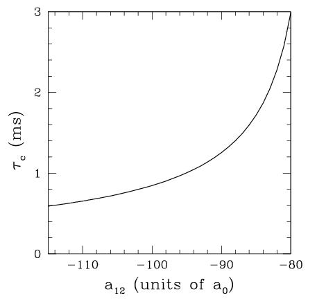
Figure 1: Capillary time $\tau_{c}$ as a function of $a_{12}$ calculated for a ⁴¹K-⁸⁷Rb cylindrical filament with $R=15,000\,a_{0}$

III.2 Equilibrium structure of a free-standing cylindrical filament

Prior to the dynamics, one has to obtain the static configuration constituting its starting point. To this end, we have computed the equilibrium structure of a free-standing cylindrical filament, i.e. $V(z)=0$ and $\omega_{\perp}=0$ in Eq. (22), taking $a_{12}=-90\,a_{0}$.

Some properties of the equilibrium filament are reported in the Table 1. They have been computed using the 1D equation for three values of the linear density $N_{1}/L$, where $L$ is the length of the filament, which yield three different radial density profiles and sizes. In the table, the sharp radius $R$ of the cylinder is defined as the radial distance at which $\rho=\rho_{c}/2$, $\rho_{c}=N_{1}/L$ being the density along the filament axis. Notice that this definition is strictly appropriate in the case of a thick filament consisting in a bulk region with flat-top density equal to the equilibrium density in the homogeneous system separated from the vacuum by a finite-width surface profile, the surface width being much smaller than $R$. In the present case, this definition of radius is somewhat arbitrary due to the Gaussian-like nature of the transverse density profile, as shown in the following. The capillary times have been computed from Eq. (24) using for the filament radius either the sharp radius, or the equilibrium value for $\sigma$. The definition and values of the Rayleigh-Plateau instability length $\lambda_{c}$ in Table 1 are discussed in Sec. III.C.

	$N_{1}/L$ ($a_{0}^{-1}$)	$E/(N_{1}+N_{2})$ $(Ha)$	$\sigma$ $(a_{0})$	$R$ $(a_{0})$	$\tau_{c}^{\sigma}$ (ms)	$\tau_{c}^{R}$ (ms)	$\lambda_{c}$ $(a_{0})$	$2\pi R/\lambda_{c}$
	0.095	-1.295 $10^{-14}$	16045	13368	1.101	0.837	72910	1.15
	0.159	-2.189 $10^{-14}$	17390	14487	1.243	0.945	111300	0.82
	0.238	-2.759 $10^{-14}$	19715	16423	1.500	1.141	160680	0.64

Table 1: Equilibrium properties for three filaments with $a_{12}=-90\,a_{0}$ calculated with the 1D equation. Atomic units are used for lengths and energies, times are expressed in ms.

To verify the validity of the approximations underlying the use of Eqs. (22) and (23), we have also computed the equilibrium structure for the same cylindrical filament using instead the 3D Eqs. (4). The transverse profile of the filament computed with the two methods (1D and 3D equations) for $N_{1}/L=0.159\,a_{0}^{-1}$ is shown in Fig. 2, where one may see a good agreement between both and conclude that it is fairly Gaussian-like. Notice that the density profile of the filament is very different from that of a macroscopic incompressible liquid cylinder characterized by a flat-top density profile encompassing a bulk region with a nearly constant density, and a narrow surface region whose width is determined by the surface tension Pol21 , as those found for classical viscid fluidsEgg08 and superfluid ⁴HeAnc23 filaments. Here, we have instead an all-surface, highly compressible cylindrical filament. Experimentally, it is easier to realize this Gaussian-like system, since the very large number of atoms required to create a flat-top density profile is difficult to reach due to the increasing role played by three-body losses which rapidly deplete the system.

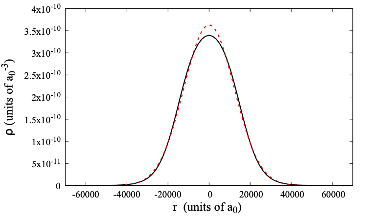
Figure 2: Density profile for the filament with $N_{1}/L=0.159\,a_{0}^{-1}$ plotted in the transverse direction (perpendicular to the filament axis). The total density $\rho_{1}+\rho_{2}$ is shown in units of $a_{0}^{-3}$. Solid line: 3D model; dashed line: 1D model.

	$N_{1}/L$ ($a_{0}^{-1}$)	$E/(N_{1}+N_{2})$ $(Ha)$	$\sigma$ $(a_{0})$	$R$ $(a_{0})$	$\tau_{c}^{\sigma}$ (ms)	$\tau_{c}^{R}$ (ms)	$\lambda_{c}$ $(a_{0})$	$2\pi R/\lambda_{c}$
	0.095	-1.333 $10^{-14}$	15769	12951	1.101	0.837	73700	1.10
	0.159	-2.214 $10^{-14}$	17917	15650	1.243	0.945	103560	0.95
	0.238	-2.815 $10^{-14}$	21019	19178	1.500	1.141	135200	0.89

Table 2: Equilibrium properties for three filaments with $a_{12}=-90\,a_{0}$ calculated with the 3D equations. Atomic units are used for lengths and energies, times are expressed in ms.

We report in Table 2 some equilibrium properties calculated using the 3D equations for the same filaments as in Table 1. The width $\sigma$ has been estimated by assuming that the transverse wave function is a Gaussian as in Eq. (19), i.e. $\sigma=\sqrt{N_{1}/(\pi L\rho_{c})}$, where $\rho_{c}$ is the uniform density value along the filament axis. A comparison with Table 1 shows an overall good agreement between 1D and 3D models, albeit with some differences in the case of the thicker filament.

III.3 Capillary instability

We have verified by real-time dynamics that a cylindrical quantum liquid filament is indeed unstable against a small initial axial perturbation of the density with a sufficiently large wavelength, as predicted by the Rayleigh theory. We have used both approaches, i.e., that based on the 3D MF-LHY equations and the one based on the effective 1D equation. For a classical incompressible fluid, any perturbation with wavelength $\lambda$ greater than $2\pi R$ makes the system unstable allowing the surface tension to break the cylinder into droplets, thus decreasing the surface energy of the system.

We have studied the instability threshold for the three filaments whose properties are summarized in Tables 1 and 2. To this end, we have applied a weak axial perturbation on the transverse width of the filament of the form

$$\sigma(z)=\sigma_{0}\left[1-\epsilon\,cos\left(\frac{2\pi z}{L}\right)\right]\,,$$ (26)

where $L$ is the total length of the filament, $\sigma_{0}$ is the equilibrium value for the filament transverse size, and $\epsilon\ll 1$. We then let the system evolve in time; if $L$ is smaller than a critical value $\lambda_{c}$, the filament remains intact and one simply observes small amplitude surface oscillations due to the initial perturbation. However, above this critical value, the amplitude of the initial perturbation starts to grow, a neck develops and eventually the filament breaks into droplets. We determined in this way the value of $k=2\pi/L$ that makes the filaments unstable, i.e. the critical wavelength $\lambda_{c}=2\pi/k$ (see Tables 1-2). We recall that linear theory for a classical fluid filament predicts $(2\pi/\lambda_{c})R=1$ Ray79 ; this is only approximately true for the liquid filaments investigated here, where the ratio $R/\lambda_{c}$ turns out not to be universal but weakly depends on the linear density of the system or, equivalently, on the radius, as shown in Tables 1-2. We remark that this is not a limitation due to the nanoscopic nature of our system; in fact, calculations on nanoscopic ⁴He superfluid liquid filaments Anc23 yielded the universal result of linear theory for inviscid classical fluids. Rather, it is likely due to the all-surface nature of the filaments investigated here, and the very large compressibility of quantum liquids Pol21 ; the classical, linear theory assumes instead an incompressible fluid and a sharp surface filament.

The actual time taken for the filament to break into droplets depends upon the amplitude of the initial density perturbation. It is defined as the time $\tau_{b}$ it takes for the wave amplitude with the largest frequency to grow up to the value of the filament radius, thus breaking it Dum08 ; Hoe13 . For a given time, the amplitude of a perturbation, with some given wavevector $k$, evolves as

$$\delta(t)=\delta_{0}e^{\omega(k)t}\,.$$ (27)

We have computed the dynamics of neck shrinking by monitoring during the real-time evolution the quantity $\delta(t)=(R_{max}-R_{min})/2$, where the radii $R_{max}$ and $R_{min}$ are measured at the two positions corresponding to a crest (maximum) and a valley (minimum) in the filament surface. As for ⁴He filamentsAnc23 , we have first checked that the exponential law is indeed strictly followed by the simulations, and from the calculated values for $\delta(t)/\delta_{0}$ we have computed $\omega$ as a function of the adimensional quantity $kR$. The results are shown in Fig. 3 for the filament with linear density $N_{1}/L=0.159\,a_{0}^{-1}$. It appears that there is a maximum frequency $\omega_{max}=0.84/\tau_{c}$ at about $kR=0.7$, i.e., the actual breaking of a filament subject to a most general perturbation will be dominated by the fastest mode with $\omega=\omega_{max}$ being characterized by a time constant $\tau\sim 2\pi/\omega_{max}\sim 9.3$ ms.

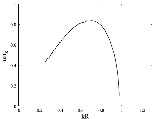
Figure 3: Plot of $\omega\tau_{c}$ vs. $kR$ for the filament with $N_{1}/L=0.159\,a_{0}^{-1}$.

The actual dynamics of the instability is provided by the solutions of the time dependent equation for the filament. We use here the 3D equations described before and apply them to the $N_{1}/L=0.159\,a_{0}^{-1}$ free-standing filament, and to a filament with the same $N_{1}/L$ value laterally confined by a harmonic confinement with $\omega_{x}=\omega_{y}=2\pi(100)$ Hz. We chose a value for the wavelength corresponding to the maximum of the $\omega(k)$ curve, i.e., $kR\sim 0.7$. Similarly to what we have done when solving the 1D problem, we started the numerical simulations from the previously obtained equilibrium filament and apply a small axial perturbation with wavelength $\lambda_{c}$ and initial amplitude $\epsilon=0.05R$.

Figure 4 shows some snapshots of the filament density on a symmetry plane containing the symmetry $z$-axis. It corresponds to the evolution of the free-standing filament. It can be seen from the figure that, starting from the perturbed filament, undulations whose amplitude increases with time appear along the filament. The instability is caused by the Laplace pressure increase in constricted regions (necks), driving out the fluid and hence reducing further the neck radius. The filament evolves into higher density bulges connected by thin threads bridging adjacent bulges. At variance with the fragmentation of inviscid classical fluids and even superfluid ⁴He, where such threads eventually break up forming smaller satellite droplets, here instead they swiftly evaporate. The main droplets forming after the fragmentation execute oscillatory motion, being alternately compressed and elongated in the filament direction.

In order to check that the fragmentation dynamics of the filament is not hindered by the presence of an external potential, like the one necessary to confine the filament within a toroidal geometry, we also addressed the case where the filament is subject to a transverse harmonic confinement. This is shown in Fig. 5 for the same instants shown in Fig. 4. It appears that the dynamics of fragmentation is very similar to the case of the free-standing filament, with some visible effects of the lateral confinement on the droplet shapes (compare the last three panels in Fig. 4 and Fig.5).

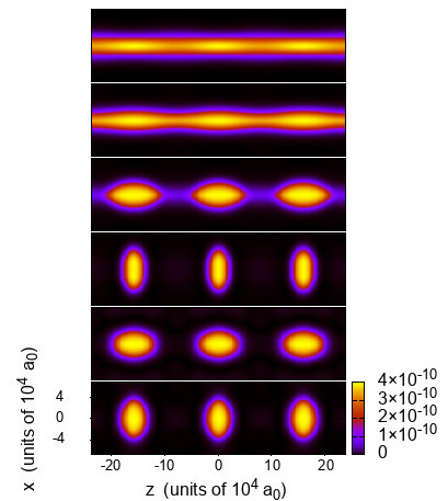
Figure 4: Snapshots from the real time evolution obtained by solving the 3D equations for a free-standing filament with $N_{1}/L=0.159\,a_{0}^{-1}$. The color bar displays the total number density in units of $a_{0}^{-3}$. The filament is initially perturbed by a periodic perturbation with $kR\sim 0.7$. From top to bottom, the snapshots are taken at $t=0,15,19,21,24$, and 27 ms.

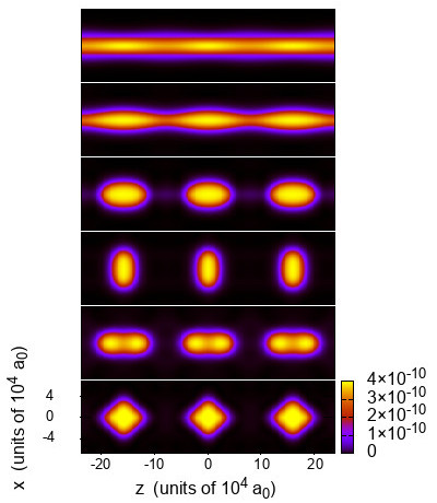
Figure 5: Snapshots from the real time evolution obtained by solving the 3D equations for a filament with $N_{1}/L=0.159\,a_{0}^{-1}$ subject to a lateral harmonic confinement as described in the text. The color bar displays the total number density in units of $a_{0}^{-3}$. The filament is initially perturbed by a periodic perturbation with $kR\sim 0.7$. From top to bottom, the snapshots are taken at $t=0,15,19,21,24,$ and 27 ms.

We have also studied the instability of thin ⁴¹K-⁸⁷Rb free-standing filaments triggered by a more general initial axial perturbation. To do so, we consider a “random” modulation of the initial transverse section $\sigma(z)$ obtained by superimposing two sinusoidal modulations with incommensurate periods, one with a short period $d_{s}$, and another with a longer period $d_{l}$ (see, e.g., Ref. Fal07, ):

$$\sigma(z)=\sigma_{0}\,\{1+\epsilon[sin(\pi z/d_{s})^{2}+sin(\pi z/d_{l})^{2}-1]\}\,,$$ (28)

where $\sigma_{0}$ is the width of the equilibrium filament.

An infinite quasi-periodic disorder results when the ratio $d_{l}/d_{s}$ is an irrational number. We choose the golden ratio $\phi=(\sqrt{5}+1)/2$ for such a number. Since our simulations use a finite box with periodic boundary conditions, to make the above expression of $\sigma$ consistent with the use of PBC along the $z$-axis one must approximate this number by the ratio of two integer numbers, the largest one providing the total length of the periodic cell used in the calculation. Here we approximate $\phi$ with the ratio of two successive numbers in the Fibonacci sequence, $d_{l}/d_{s}=F_{j+1}/F_{j}$ Mod09 , which notoriously converges towards the golden ratio for large values of $j$. In particular, we take $L=8\,\lambda_{c}$ where $\lambda_{c}$ is the instability threshold for filament breaking. We consider the case $N_{1}/L=0.159\,a_{0}^{-1}$, so that $\lambda_{c}=111300$ (see Table I). We choose the two adjacent elements $13,21$ in the Fibonacci sequence, so that $d_{s}=42400\,a_{0}$ and $d_{l}=68492\,a_{0}$. With this choice, $L=21\,d_{s}=13\,d_{l}$, making the applied perturbation satisfying the periodic boundary conditions. We also took $\epsilon=0.06R$. Given the large size of the system, which makes the full 3D calculations very computationally demanding, we have employed here the 1D effective equation.

The time evolution obtained by starting the dynamics from this initial state is shown in the sequence of snapshots displayed in Fig. 6. It appears that the filament undergoes fragmentation, leading to the appearance of five droplets. This fragmentation pattern is what is expected from an undulation with wavelength $\lambda=L/5=1.6\times 10^{5}\,a_{0}$, where $L$ is the length of the filament in the figure, which corresponds to a value $kR\sim 0.7$, close to the maximum of the curve shown in Fig. 3. Therefore, as expected, the fragmentation dynamics is eventually dominated by the fastest mode compatible with the length of our simulation cell, resulting in the filament fragmentation into regularly arranged, identical droplets. Once formed, they execute a series of large amplitude oscillations, being alternately compressed and elongated in the filament direction. Eventually, these oscillations will be damped by any residual friction, resulting in a necklace of identical, equidistant quantum droplets.

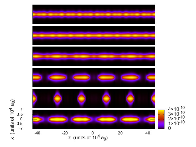
Figure 6: Snapshots from the real time evolution obtained by solving the 1D equation for a free-standing filament with $N_{1}/L=0.159\,a_{0}^{-1}$. The color bar displays the total number density in units of $a_{0}^{-3}$. The filament is subject to an initial, most generic perturbation, as described in the text. From top to bottom, the snapshots are taken at times $t=0,8,13,15,17$, and 19 ms.

III.4 Possible supersolid behavior of the fragmented state

From the previous results, the lowest energy state resulting from the fragmentation of a quantum liquid filament appears to be made of regularly arranged droplets, the inter-droplet spacing being determined by the wavelength of the fastest mode that matches the filament length $L$.

When the number of atoms of each species in the mixture is such that the local densities satisfy the equilibrium condition $N_{1}/N_{2}=\sqrt{g_{22}/g_{11}}$, the resulting droplets are separated by vacuum. However, when the population ratio deviates from the optimal value, i.e., there is one species in excess, then the extra atoms in the larger component (in the following the ⁸⁷Rb species) cannot bind to the droplets, whose composition already satisfies the equilibrium ratio, and form instead a uniform halo embedding them. This dilute superfluid background is expected to provide a degree of global phase coherence to the system, unlike the case of droplets separated by vacuum where no such coherence is present between adjacent droplets. This suggests that the droplets array in the unbalanced system may display a supersolid character, i.e., coexistence of superfluidity and a periodic density modulation.

The possibility of supersolid phases in a binary Bose mixture has recently been put forward in Ref. Sac20, , where a self-bound 2D supersolid stripe-phase in a weakly interacting binary BEC with spin-orbit coupling has been proposed, being stabilized by the Lee-Huang-Yang beyond-mean-field term. In Ref. Ten22, , a single one-dimensional droplet made of a binary Bose mixture immersed into a background of the excess species and subject to periodic boundary conditions (as a model for a droplet confined in a toroidal trap), was found to display non-classical rotational inertia and thus the coexistence of rigid-body and superfluid character.

In our case, to verify the hypothesis that the fragmented state in the presence of an excess population of atoms of one species may indeed show supersolid character, we have looked for a hallmark of supersolid behavior of the modulated structures, namely a finite non-classical translational inertia. Following Refs. Pom94, ; Sep08, , we define the superfluid fraction $f_{s}$ as the fraction of particles that remain at rest in the comoving frame with a constant velocity $v_{x}$

$$f_{s}=1-\lim_{v_{x}\to 0}\frac{{\big{<}}(P_{x,1}+P_{x,2}){\big{>}}}{(N_{1}m_{1}+N_{2}m_{2})v_{x}}\,,$$ (29)

where ${\big{<}}P_{x,i}{\big{>}}=-i\hbar\int\psi_{i}^{\ast}\partial\psi_{i}/\partial x$ is the expectation value of the momentum of the $i$-th species and $(N_{1}m_{1}+N_{2}m_{2})v_{x}$ is the total momentum of the system as if all droplets were moving as a rigid body. A non-zero value for $f_{s}$ reveals global phase coherence in a periodic system like the one studied here.

The $f_{s}$ parameter should not be confused with the total superfluid fraction. For instance, in the regime where self-bound droplets form but are separated from each other by vacuum, $f_{s}$ is zero although droplets are individually superfluid, meaning that there is no global phase coherence. At variance, for an ideal superfluid filament prior to breakup, $f_{s}$ is equal to 1 since the system is homogeneous along the filament axis. Any periodic modulation should result in a finite value $0<f_{s}<1$.

We have calculated $f_{s}$ for the three ground state structures shown in Fig. 7. They refer to the case $N_{1}/L=0.159\,a_{0}^{-1}$. In the top panel the equilibrium filament is shown. The calculated value for the superfluid fraction is $f_{s}=1$, as expected. The middle panel shows the fragmented, multi-droplet state resulting from a mixture satisfying the equilibrium composition ratio when it has been subject to an initial perturbation with $kR\sim 0.7$. We find for such structure $f_{s}<0.001$. The lowest panel shows instead the case where the ⁸⁷Rb species is in excess. The chosen values of $N_{1}$ and $N_{2}$ are such that there is just a small background density due to the excess species ($\sim 2.5\%$ of the total density in the center of a droplet), as shown in Fig. 8, where a cut of the densities (⁴¹K, ⁸⁷Rb and total ⁴¹K+⁸⁷Rb densities) along the system symmetry $z$-axis is displayed. In spite of the small amount of ⁸⁷Rb density enveloping the ⁴¹K-⁸⁷Rb droplets, the resulting superfluid fraction is surprisingly large, $f_{s}=0.53$. This finite value for $f_{s}$ likely indicates a supersolid character of the droplet array.

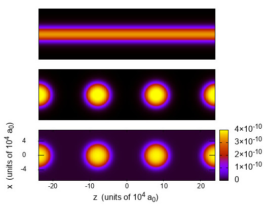
Figure 7: Lowest energy configurations for the states described in the text. Upper panel: free-standing filament prior to fragmentation; middle panel: fragmented state (balanced mixture composition); lower panel: fragmented state (unbalanced mixture composition). The color bar displays the total number density in units of $a_{0}^{-3}$.

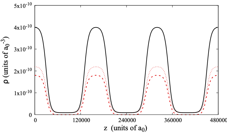
Figure 8: Density profiles along the filament symmetry $z$-axis for the droplet array shown in the lower panel of Fig. 7. Dotted line: ⁸⁷Rb density; dashed line: ⁴¹K density; solid line: total (⁴¹K+⁸⁷Rb) density.

IV Summary and outlook

We predict that a bosonic ⁴¹K-⁸⁷Rb mixture confined in a sufficiently long toroidal trap, in the regime where a self-bound liquid state forms, will undergo Rayleigh-Plateau instability and produce a necklace of droplets inside the torus. The droplets will be subject to oscillations also in the tubular confinement, although some damping in the real system is expected what drives them to rest.

In the presence of a non-equilibrated mixture, i.e. when there is one species in excess with respect to the optimal ratio $N_{1}/N_{2}=\sqrt{g_{22}/g_{11}}$, the excess species is expelled from the ⁴¹K-⁸⁷Rb filament. Due to the presence of transverse confinement, the excess part cannot evaporate but remains instead in the trap, enveloping the ⁴¹K-⁸⁷Rb liquid droplets resulting from filament fragmentation. This results in a global phase coherence between one droplet and the next, leading to a possible supersolid behavior.

This toroidal geometry is experimentally realizable and therefore our results could be compared with experiments when curvature effects can be neglected. In practice, it might be very challenging to prevent the formation of a single big droplet inside the toroidal trap during the quenching of $a_{12}$ required to reach the quantum liquid state. In this regard, it might help to look for the instability when the value of the interspecies scattering length $a_{12}$ is close to the gas-liquid transition value so that the density of the self-bound state is not much larger than that in the gas phase. In the presence of a tight confinement, the single droplet state should be energetically disfavoured with respect to the (unstable) filament configuration.

- (1) D. S. Petrov, Phys. Rev. Lett. 115, 155302 (2015).
- (2) I. Ferrier-Barbut, H. Kadau, M. Schmitt, M. Wenzel, and T. Pfau, Phys. Rev. Lett. 116, 215301 (2016).
- (3) L. Chomaz, S. Baier, D. Petter, M. J. Mark, F. Wächtler, L. Santos, and F. Ferlaino, Phys. Rev. X 6, 041039 (2016).
- (4) C. R. Cabrera, L. Tanzi, J. Sanz, B. Naylor, P. Thomas, P. Cheiney, and L. Tarruell, Science 359, 301 (2018).
- (5) G. Semeghini, G. Ferioli, L. Masi, C. Mazzinghi, L. Wolswijk, F. Minardi, M. Modugno, G. Modugno, M. Inguscio, and M. Fattori, Phys. Rev. Lett. 120, 235301 (2018).
- (6) C. D’Errico, A. Burchianti, M. Prevedelli, L. Salasnich, F. Ancilotto, M. Modugno, F. Minardi, and C. Fort, Phys. Rev. Research 1, 033155 (2019).
- (7) Z. Guo, F. Jia, L. Li, Y. Ma, J. M. Hutson, X. Cui, and D. Wang, Phys. Rev. Research 3, 033247 (2021).
- (8) J. Eggers and E. Villermaux, Rep. Prog. Phys. 71, 036601 (2008).
- (9) J. Plateau, London Edinburgh Dublin Philos. Mag. J. Sci. 14, 431 (1857).
- (10) Lord Rayleigh, Proc. London Math. Soc. s1-11, 57 (1879).
- (11) F. Ancilotto, M. Barranco, and M. Pi, J. Chem. Phys. 158, 144306 (2023).
- (12) F. Ancilotto, M. Barranco, F. Coppens, J. Eloranta, N. Halberstadt, A. Hernando, D. Mateo, and M. Pi, Int. Rev. Phys. Chem. 36, 621 (2017).
- (13) K. Sasaki, N. Suzuki and H. Saito, Phys. Rev. A 83, 053606 (2011).
- (14) V. Cikojević, E. Poli, F. Ancilotto, L. Vranjesr-Markić, and J. Boronat Phys. Rev. A 104, 033319 (2021).
- (15) L. Salasnich, A. Parola, and L. Reatto, Phys. Rev. A 65, 043614 (2002).
- (16) F. Ancilotto, M. Barranco, M. Guilleumas, and M. Pi, Phys. Rev. A 98, 053623 (2018).
- (17) C. D’Errico, M. Zaccanti, M. Fattori, G. Roati, M. Inguscio, G. Modugno, and A. Simoni, New J. Phys. 9, 223 (2007).
- (18) A. Marte, T. Volz, J. Schuster, S. Durr, G. Rempe, E. G. M. van Kempen, and B. J. Verhaar, Phys. Rev. Lett. 89, 283202 (2002).
- (19) F. Minardi, F. Ancilotto, A. Burchianti, C. D’Errico, C. Fort, and M. Modugno, Phys. Rev. A 100, 063636 (2019).
- (20) C. Staudinger, F. Mazzanti, and R. E. Zillich, Phys. Rev. A 98, 023633 (2018).
- (21) A. Ralston and H. S. Wilf, Mathematical methods for digital computers (John Wiley and Sons, New York, 1960).
- (22) R. C. Tolman, J. Chem. Phys. 17, 333 (1949).
- (23) E. Blokhuis and J. Kuipers, J. Chem. Phys. 124, 074701 (2006).
- (24) Ch. Dumouchel, Exp. Fluids 45, 371 (2008).
- (25) J. Hoepffner and G. Paré, J. Fluid Mech. 734, 183 (2013).
- (26) L. Fallani, J. E. Lye, V. Guarrera, C. Fort, and M. Inguscio, Phys. Rev. Lett. 98, 130404 (2007).
- (27) M. Modugno, New J. Phys. 11, 033023 (2009).
- (28) R. Sachdeva, M. N. Tengstrand, and S. M. Reimann, Phys. Rev. A 102, 043304 (2020).
- (29) M. N. Tengstrand and S. M. Reimann, Phys. Rev. A 105, 033319 (2022).
- (30) Y. Pomeau and S. Rica, Phys. Rev. Lett. 72, 2426 (1994).
- (31) N. Sepúlveda, C. Josserand, and S. Rica, Phys. Rev. B 77, 054513 (2008).