Preference Inference from Demonstration in Multi-objective Multi-agent Decision Making

Abstract

It is challenging to quantify numerical preferences for different objectives in a multi-objective decision-making problem. However, the demonstrations of a user are often accessible. We propose an algorithm to infer linear preference weights from either optimal or near-optimal demonstrations. The algorithm is evaluated in three environments with two baseline methods. Empirical results demonstrate significant improvements compared to the baseline algorithms, in terms of both time requirements and accuracy of the inferred preferences. In future work, we plan to evaluate the algorithm’s effectiveness in a multi-agent system, where one of the agents is enabled to infer the preferences of an opponent using our preference inference algorithm.

Keywords Multi-objective Reinforcement Learning $\cdot$ Preference Inference $\cdot$ Dynamic Weight Multi-objective Agent $\cdot$ Multi-agent System $\cdot$ Opponent Modelling

1 Introduction

In a multi-objective decision-making process, the agent receives reward vectors for different objectives. The utility function is used to make trade-offs between competing objectives by evaluating the reward vector as a utility scalar. In the existing literature, the most frequently used approach to get utility scalar is linear scalarization (Castelletti et al., 2013; Khamis and Gomaa, 2014; Ferreira et al., 2017; Lu et al., 2022). In linear scalarization, the weight over the reward is referred to as the preference. However, giving a precise numerical preference is not always intuitive for users. For example, consider a case where a portfolio manager selects stocks based on their weighting of minimizing risk and maximizing profits. He/she might want to give a higher weighting to maximize profits but a specific value is hard to determine. A small error in their preference can result in a significantly different policy which may lead to a sub-optimal solution. However, although it is difficult to numerically name the preference, a user can often demonstrate their preferences. Preference Inference (PI) methods that use demonstration are therefore helpful when solving such problems.

Furthermore, in a multi-agent multi-objective decision-making process, if some agent can use the PI mechanism to infer other agents’ preferences, it could gain information about the other agents. The knowledge of others’ preferences can provide an advantage to these "wise" agents.

2 Preference Inference

PI is to infer a set of weights that are used to scalarize a reward vector during the multi-objective decision-making process. This is similar to inverse reinforcement learning (IRL), which infers the reward function by finding a set of linear parameters that scalarize state-relevant features. There are two assumptions:

• The trajectories observed are from the optimal policy or near-optimal policy. This is a widely accepted assumption in existing literature for both IRL (Ng et al., 2000; Ziebart et al., 2008; Wulfmeier et al., 2015) and PI (Takayama and Arai, 2022).

• Based on the first assumption, given either optimal or near-optimal policy, the average reward trajectory is solely determined by preferences and environment transitions.

The PI problem happens when we are given a point assumed to be on the Pareto optimal set (POS) based on some unknown weights for the utility function, and we would like to know what exactly the weights are. For more realistic scenarios, we also consider dominated points that are close to the points on the POS, known as sub-optimal policies to test the PI algorithm. By adding sub-optimal noise to the data, we ensure that the inference model is robust on sub-optimal reward trajectories.

We first use the dynamic weight reinforcement learning (DWRL) agent to generate behaviour trajectories (Källström and Heintz, 2019). We then propose the dynamic weight-based preference inference (DWPI) algorithm to infer the preferences of the agent for different behaviour trajectories. The training process of the DWPI algorithm is presented in Figure 1.

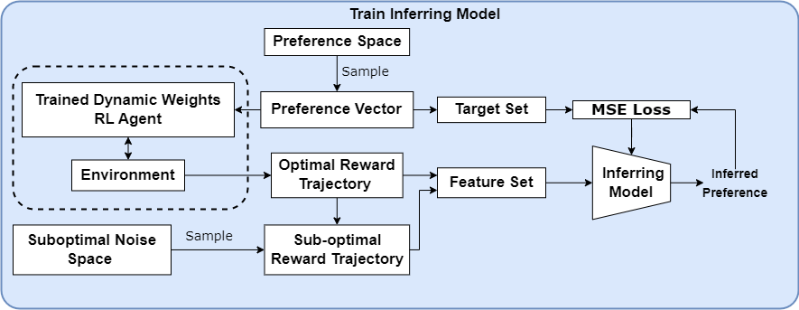
Figure 1: DWPI Training Phase

The DWRL agent takes the preference vector as part of the state so that it can change its behavior pattern during runtime by changing the preference. Given the interaction between a trained DWRL agent and the environment, a set of optimal reward trajectories are generated. The trajectory set is augmented by adding random sampled sub-optimal noise to be the training set of the inference model. The inference model is trained under the supervised learning paradigm by inputting the reward trajectory and predicting the corresponding preference.

Algorithm 1 Dynamic Weight Preference Inference Algorithm

  Initialize inferring model $\mathcal{I}$, sub-optimal noise space $\mathcal{SN}$, environment $\mathcal{E}$, and preference space $\Omega$

  Load the trained dynamic weights RL agent $AG$

  Initialize feature set $X$, target set $Y$

  while not enough entries in $X$ do

     Sample a preference vectors $\bm{\omega}$ from $\Omega$

     $AG$ plays one episode with $\bm{\omega}$, generates reward trajectory $\bm{\tau_{r}}$

     Sample a noise vector $\bm{\delta}$ from $\mathcal{SN}$

     Store the noisy reward trajectory $\bm{\tau_{r}}+\bm{\delta}$ in $X$, store $\bm{\omega}$ in $Y$

  end while

  while $\mathcal{I}$ not converge do

     Sample batch from $X$ to train the inferring model, loss $\mathcal{L}=\lVert\hat{\bm{\omega}}-\bm{\omega}\rVert$

  end while

We evaluate our algorithm in three environments: Convex Deep Sea Treasure(Mannion et al., 2017), Traffic(Källström and Heintz, 2019), and Item Gathering(Källström and Heintz, 2019) and compared to two benchmarks projection method (PM) (Ikenaga and Arai, 2018) and multiplicative weights apprenticeship learning (MWAL) (Takayama and Arai, 2022). Our method outperforms the baseline methods by both time efficiency (Figure 2) and PI performance (Table 1). The experiments are implemented with Python 3.9, TensorFlow version 2.3.0, and run on a machine with 11th Gen Intel(R) Core(TM) i7-1165G7 2.80GHz CPU.

Figure 2: Time Efficiency Comparison

Table 1: Performance Improvement

Environment		Traffic		Item Gathering
KL-divergence		PM	MWAL	PM	MWAL
Optimal Demo	DWPI	90.8%$\uparrow$	99.56%$\uparrow$	98.01%$\uparrow$	99.13%$\uparrow$
Sub-optimal Demo	DWPI	89.55%$\uparrow$	99.53%$\uparrow$	96.89%$\uparrow$	99.25%$\uparrow$
Mean Squared Error		PM	MWAL	PM	MWAL
Optimal Demo	DWPI	97.7%$\uparrow$	99.8%$\uparrow$	85.91%$\uparrow$	98.1%$\uparrow$
Sub-optimal Demo	DWPI	94.13%$\uparrow$	99.83%$\uparrow$	83.81%$\uparrow$	98.9%$\uparrow$
Utility		PM	MWAL	PM	MWAL
Optimal Demo	DWPI	60.56%$\uparrow$	98.93%$\uparrow$	90.67%$\uparrow$	82.62%$\uparrow$
Sub-optimal Demo	DWPI	71.87%$\uparrow$	90.60%$\uparrow$	99.85%$\uparrow$	94.50%$\uparrow$

The results of the evaluation show that the DWPI algorithm performs well in terms of inference accuracy.

3 Opponent Preference Modelling

In future work, we will utilize the DWPI algorithm in the multi-agent environment to enable an agent to gain knowledge of other agents’ preferences to gain an advantage over them.

It will be evaluated in two environments. The first one is the Wolfpack environment (Leibo et al., 2017), where two predator agents try to capture randomly moving prey. If the capture happens when the Manhattan distance between the two predators $dist\leq 3$, it is determined as cooperation or competition when $dist>3$.

The second environment is the multi-agent item gathering modified from (Källström and Heintz, 2019). Two RL agents move in the grid world to gather randomly distributed blocks with three different colors, i.e. green, red, and yellow. Each agent has a preference weight vector over the color of the blocks.

Two sets of experiments will be done in each environment. The first experiment is between two normal agents while the second experiment is between a normal agent and a wiser agent which is able to infer the other’s preference. The performance of the agents will be analyzed to check whether the inference mechanism will help the wiser agent gain advantages during the games.

4 Conclusion

We propose the DWPI algorithm to infer preference from demonstrations in the multi-objective decision-making process. We further evaluate the utility of this algorithm for enhancing an agent in the multi-agent system. With our PI model, an agent can know its opponent better and therefore achieve better performance on its target. For future work, we would like to evaluate the opponent preference modeling performance in multi-agent systems. The extension of the DWPI algorithm to infer a non-linear preference is also a direction that we are interested in.

References

- Castelletti et al. [2013] Andrea Castelletti, Francesca Pianosi, and Marcello Restelli. A multiobjective reinforcement learning approach to water resources systems operation: Pareto frontier approximation in a single run. Water Resources Research, 49(6):3476–3486, 2013.
- Khamis and Gomaa [2014] Mohamed A Khamis and Walid Gomaa. Adaptive multi-objective reinforcement learning with hybrid exploration for traffic signal control based on cooperative multi-agent framework. Engineering Applications of Artificial Intelligence, 29:134–151, 2014.
- Ferreira et al. [2017] Paulo Victor R Ferreira, Randy Paffenroth, Alexander M Wyglinski, Timothy M Hackett, Sven G Bilén, Richard C Reinhart, and Dale J Mortensen. Multi-objective reinforcement learning-based deep neural networks for cognitive space communications. In 2017 Cognitive Communications for Aerospace Applications Workshop (CCAA), pages 1–8. IEEE, 2017.
- Lu et al. [2022] Junlin Lu, Patrick Mannion, and Karl Mason. A multi-objective multi-agent deep reinforcement learning approach to residential appliance scheduling. IET Smart Grid, 2022.
- Ng et al. [2000] Andrew Y Ng, Stuart J Russell, et al. Algorithms for inverse reinforcement learning. In Icml, volume 1, page 2, 2000.
- Ziebart et al. [2008] Brian D Ziebart, Andrew L Maas, J Andrew Bagnell, Anind K Dey, et al. Maximum entropy inverse reinforcement learning. In Aaai, volume 8, pages 1433–1438. Chicago, IL, USA, 2008.
- Wulfmeier et al. [2015] Markus Wulfmeier, Peter Ondruska, and Ingmar Posner. Deep inverse reinforcement learning. CoRR, abs/1507.04888, 2015.
- Takayama and Arai [2022] Naoya Takayama and Sachiyo Arai. Multi-objective deep inverse reinforcement learning for weight estimation of objectives. Artificial Life and Robotics, pages 1–9, 2022.
- Källström and Heintz [2019] Johan Källström and Fredrik Heintz. Tunable dynamics in agent-based simulation using multi-objective reinforcement learning. In Adaptive and Learning Agents Workshop (ALA-19) at AAMAS, Montreal, Canada, May 13-14, 2019, pages 1–7, 2019.
- Mannion et al. [2017] Patrick Mannion, Sam Devlin, Karl Mason, Jim Duggan, and Enda Howley. Policy invariance under reward transformations for multi-objective reinforcement learning. Neurocomputing, 263:60–73, 2017.
- Ikenaga and Arai [2018] Akiko Ikenaga and Sachiyo Arai. Inverse reinforcement learning approach for elicitation of preferences in multi-objective sequential optimization. In 2018 IEEE International Conference on Agents (ICA), pages 117–118. IEEE, 2018.
- Leibo et al. [2017] Joel Z Leibo, Vinicius Zambaldi, Marc Lanctot, Janusz Marecki, and Thore Graepel. Multi-agent reinforcement learning in sequential social dilemmas. arXiv preprint arXiv:1702.03037, 2017.