Ordinary Differential Equation-based
MIMO Signal Detection

Abstract

Inspired by the emerging technologies for energy-efficient analog computing and continuous-time processing, this paper proposes a continuous-time minimum mean squared error (MMSE) estimation for multiple-input multiple-output (MIMO) systems based on an ordinary differential equation (ODE). We derive an analytical formula for the mean squared error (MSE) at any given time, which is a primary performance measure for estimation methods in MIMO systems. The MSE of the proposed method depends on the regularization parameter, which affects the convergence properties. In addition, this method is extended by incorporating a time-dependent regularization parameter to enhance convergence performance. Numerical experiments demonstrate excellent consistency with theoretical values and improved convergence performance due to the integration of the time-dependent parameter. Other benefits of the ODE are also discussed in this paper. Discretizing the ODE for MMSE estimation using numerical methods provides insights into the construction and understanding of discrete-time estimation algorithms. We present discrete-time estimation algorithms based on the Euler and Runge-Kutta methods. The performance of the algorithms can be analyzed using the MSE formula for continuous-time methods, and their performance can be improved by using theoretical results in a continuous-time domain. These benefits can only be obtained through formulations using ODE.

I Introduction

In future wireless communication systems beyond 5G and 6G, it is expected that massive connectivity can be achieved through the use of ultra-high-speed and large-capacity communication technologies [2]. With the number of mobile devices increasing annually, the traffic and computational loads at the base stations are becoming heavier. There are still several implementation challenges that need to be resolved to meet the demand for large-scale signal processing at base stations in next-generation wireless network systems [3]. In particular, typical signal detection methods in multiple-input multiple-output (MIMO) systems, such as zero-forcing and minimum mean squared error (MMSE) [4] detection methods, depend on centralized processing at the base station and require heavy computational burden, which generally requires cubic time complexity. Significant signal detection loads at the base station have become a major bottleneck in the implementation of next-generation systems [2]. Massive parallel computations with detector hardware [5] may be a potential solution. However, this method requires large-scale circuits and results in a significant energy consumption. Therefore, development of novel signal processing methods are necessary to achieve a reasonable signal detection performance with high energy efficiency. One possibility to ease the bottleneck is to reconsider analog-domain signal processing [1, 6, 7].

Also in the field of deep learning (DL), one of the main concerns of researchers is computational efficiency, which refers to the number of operations per unit of energy consumption per unit time [8, 9, 10]. Training large amounts of data on models with numerous parameters is becoming increasingly important. Today’s deep learning largely depends on the use of graphics processing units (GPUs) but many accesses between memory and the processing units lead to severe energy and time consumption. Analog-domain computation has been proposed as a solution and device development for practical applications is currently in progress [10]. Deep learning on analog devices can enable in-memory computations, that is, the computation is executed on memory itself resulting in elimination of data transfer between the memory and processing units. Most deep learning processes consist of tensor-tensor (including matrix-matrix and matrix-vector) products. The product process can be replaced by parallel operations on an analog device [11]. This operation enables more computationally efficient deep learning than GPUs [9].

Analog optical computing has also been reported to enable energy-efficient neural networks (NNs) [12]. A photonic chip-based NN proposed by [13] has several advantages such as high computational efficiency, scalability, and stability. A recent study reported a complex-valued NN on a photonic chip as proposed by Zhang et al. [14]. Additionally, optical computations are expected to play an important role for solving large-scale problems such as combinatorial optimization or probabilistic graphical models [15]. The development of photonic integrated circuits is also an active research area [16].

The aforementioned studies have inspired us to explore the potential of analog-domain signal processing for applications beyond deep neural networks such as wireless communication networks, where the most processes consists of matrix-vector product as well as the deep learning. Analog computers typically consist of analog adders, multipliers, integrators, and other nonlinear devices, and can simulate both linear and nonlinear ordinary differential equations (ODEs). If one can formulate a high-dimensional signal detection task as a continuous time dynamical system, it can potentially be implemented using analog devices, which could provide highly energy-efficient signal processing.

In this paper, we revisit analog-domain computing as a tool to overcome the computing bottleneck at the base station in wireless communications, and explore new signal detection methods. We present a continuous-time MMSE signal detection method for MIMO systems, which is derived from gradient flow dynamics [17] based on the least square objective function and described by a form of ODE. The proposed method mainly involves matrix-vector products, which makes it easy to implement in hardware. By utilizing the ODE representation, we can obtain theoretical analyses of the ODE-based MMSE detection method for MIMO signals. To the best of our knowledge, there are no relevant proposals or analyses in the previous literature. Analog computing for high-dimensional signal processing is still a developing technology from a hardware perspective. However, analyzing the proposed method can be a meaningful step towards advancing analog-domain high-dimensional signal processing for wireless communications in the future.

Continuous-time dynamical systems provide an added advantage for signal processing tasks by offering insight into the discrete-time algorithms for solving the task. This approach can serve as a complementary technique to traditional discrete-time systems, and can lead to the development of more efficient discrete-time algorithms for signal processing tasks. This relationship can be observed in the recently proposed neural ODE [18], which is an ODE that includes an NN, that is, its dynamics can be learned from data. Any numerical solver, such as the Euler and Runge-Kutta methods [19], can be used for discretizing a continuous-time dynamical system and solve high-dimensional neural ODE. The discretization by solvers provides benefits such as the controllable trade-off between accuracy and speed in inference algorithms and appropriate adjustment of step size for discretization.

Indeed, discretization can provide benefits not only for neural ODEs but also for general continuous-time dynamical systems. The process of discretizing continuous-time dynamical systems allows for a deeper understanding of the properties of the resulting discrete-time algorithms. Furthermore, it can lead to the development of novel discrete-time procedures that cannot be created solely from a discrete-time perspective.

On the basis of this background, this paper also presents discrete-time MMSE signal detection algorithms for MIMO systems. This can be achieved by discretization of ODE using numerical solutions. This paper mainly deals with the Euler method- and Runge-Kutta method-based algorithms. Construction of a solution method considering numerical stability and flexible selection of the step size of the solution method enables the development of high-performance algorithms. Conventional detection algorithms such as [20] and [21] have no mention of the above viewpoints. The theoretical analysis of the continuous-time detection method is also useful in discrete-time algorithms. It enables a detailed analysis of the convergence behavior and improvement in the convergence performance of the algorithms. These benefits indicate the potential for continuous-time signal processing as a novel construction methodology for discrete-time algorithms.

The flow of discussion and derivation in this paper is summarized in Fig. 1. The main contributions are as follows.

1. We propose a continuous-time MMSE detection method for MIMO systems derived from gradient flow dynamics based on the regularlized least square objective function. The method includes a regularization parameter that controls convergence behavior of the estimation method. We show the stability of the proposed method.

2. An analytical formula of mean squared error (MSE), which is the principal performance measure of signal detection methods, is derived in a closed form. The formula is based on the eigenvalue decomposition of the Gram matrix. From the MSE formula, we immediately derive the asymptotic MSE. These analyses enable us to track the quality of the estimation at any time instant.

3. We introduce a time-dependent regularization parameter for the proposed continuous-time MMSE detection method to improve convergence performance. An analytical MSE formula for the time-dependent system can be derived also for the time-dependent system. We optimize the time-dependent regularization parameter in terms of the convergence performance by using the analytical results.

4. Discrete-time MMSE detection algorithms are derived by discretizing ODE and applying numerical methods. We present methods on the basis of Euler method and recently proposed Runge-Kutta Chebyshev descent method [22]. These algorithms can be implemented with comparable computational costs.

5. The benefits on the discrete-time algorithms obtained from theoretical analysis for continuous-time methods are presented. MSE performance of the discrete-time algorithms becomes tractable by using the MSE formula for the continuous-time detection method. In addition, the performance improvement of the discrete-time algorithms can be achieved by introducing the time-dependent regularization parameter that is optimized for the continuous-time system.

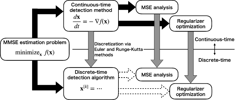
Figure 1: Flow of the discussion in this paper. We propose continuous-time MMSE detection method for MIMO systems, analyze the MSE performance, and apply regularlizer optimization. Discrete-time detection algorithm can be derived by discretization of the continuous-time method, providing the analysis and performance improvement of the algorithm.

The remainder of this paper is organized as follows. We introduce the mathematical notations and system model in Section II. Sections III–V address MIMO signal detection in analog domain, which is described by ODE. The signal processing method is proposed in Section III. Some theoretical properties of this method can be derived, as discussed in Section IV. In Section V, we demonstrate that the performance of this method can be improved by introducing a time-dependent regularizer. Section VI presents discrete-time signal detection algorithms derived via ODE. Benefits given by constructing a continuous-time method using ODE on the discrete-time algorithms are summarized in Section VII. Finally, Section VIII concludes the paper.

II Preliminaries

II-A Notation

In the rest of the paper, we use the following notation. Superscript $(\cdot)^{\mathrm{H}}$ denotes the Hermitian transpose. The zero vector and identity matrix are represented by $\bm{0}$ and $\bm{I}$, respectively. The Euclidean ($\ell_{2}$) norm is $\|\cdot\|$. The complex circularly symmetric Gaussian distribution $\mathcal{CN}(\bm{0},\bm{\Sigma})$ has a mean vector $\bm{0}$ and a covariance matrix $\bm{\Sigma}$. The expectation and trace operators are $\mathbb{E}[\cdot]$ and $\mathrm{Tr}[\cdot]$, respectively. The diagonal matrix is given by $\mathrm{diag}[\ldots]$ with the diagonal elements shown in square brackets. The matrix exponential $\exp(\bm{A})$ for a matrix $\bm{A}$ is defined by $\exp(\bm{A}):=\sum_{k=0}^{\infty}\frac{1}{k!}\bm{A}^{k}$.

II-B First-order Linear ODE

Consider a linear ODE with a constant matrix coefficient:

$$\frac{d\bm{y}(t)}{dt}=\bm{A}\bm{y}(t),$$ (1)

where $t\geq 0$ and $\bm{A}$ is a matrix that is independent of $\bm{y}(t)$ and $t$. This ODE can be solved analytically using a matrix exponential [19]. The solution is given by

$$\bm{y}(t)=\exp(\bm{A}t)\bm{y}(0),$$

where $\bm{y}(0)$ denotes the initial value of $\bm{y}(t)$.

The continuous-time dynamical system in (1) is asymptotically stable if $\bm{y}(t)$ converges to the origin $\bm{0}$ as $t\to\infty$ for all initial conditions $\bm{y}(0)$ [19]. The system is stable if and only if the real parts of all the eigenvalues of the matrix $\bm{A}$ are negative.

II-C System Model

In this paper, we consider the following MIMO channel model:

$$\bm{y}=\bm{Hs}+\bm{w},$$ (2)

where $\bm{y}\in\mathbb{C}^{m}$ is the received signal, $\bm{H}\in\mathbb{C}^{m\times n}$ is the channel matrix, $\bm{s}\in\mathbb{C}^{n}$ is the transmitted signal that follows $\mathcal{CN}(\bm{0},\bm{I})$, and $\bm{w}\in\mathbb{C}^{m}$ is the measurement noise that follows $\mathcal{CN}(\bm{0},\sigma^{2}\bm{I}$). In the following, the channel matrix $\bm{H}$ is assumed not to be a zero matrix.

A linear estimate $\hat{\bm{s}}:=\bm{Wy}$ for MIMO systems is characterized by the matrix $\bm{W}\in\mathbb{C}^{n\times m}$, which is determined according to each estimation method. Matrix $\bm{W}$ for MMSE signal detection [4] can be obtained by minimizing the MSE given by $\mathbb{E}[\|\bm{Wy}-\bm{s}\|^{2}]$. The resulting MMSE estimate is derived as

$$\hat{\bm{s}}=\left(\bm{H}^{\mathrm{H}}\bm{H}+\sigma^{2}\bm{I}\right)^{-1}\bm{H}^{\mathrm{H}}\bm{y}.$$ (3)

III Continuous-time MMSE Estimation

This paper considers a gradient flow for the MMSE estimation and describes the evolution of the estimate in continuous-time systems.

A function

$$f(\bm{x}):=\|\bm{y}-\bm{Hx}\|^{2}+\eta\|\bm{x}\|^{2},$$ (4)

where $\eta\in\mathbb{R}$ and $\eta>0$, can be regarded as the regularized least square objective function for MMSE signal detection because the unique stationary point of $f(\bm{x})$ coincides with the MMSE estimate (3) when $\eta=\sigma^{2}$ [23]. The scalar value $\eta$ in (4) behaves as a regularization parameter. The gradient vector of $f(\bm{x})$ is given by

$$\nabla f(\bm{x})=(\bm{H}^{\mathrm{H}}\bm{H}+\eta\bm{I})\bm{x}-\bm{H}^{\mathrm{H}}\bm{y}.$$ (5)

In this paper, we consider gradient flow [17, 24] in terms of the objective function (4). Subsequently, we obtain the estimate $\bm{x}(t)$ of the transmitted signal $\bm{s}$ at time $t\geq 0$ that evolves according to the ODE

$$\frac{d\bm{x}(t)}{dt}=-\nabla f(\bm{x}(t))=-(\bm{H}^{\mathrm{H}}\bm{H}+\eta\bm{I})\bm{x}(t)+\bm{H}^{\mathrm{H}}\bm{y}.$$ (6)

We further assume the initial condition $\bm{x}(0)=\bm{H}^{\mathrm{H}}\bm{y}$, which corresponds to a matched filter detector [25]. We refer to the proposed signal detection method based on the ODE (6) as Ordinary Differential Equation-based MMSE (ODE-MMSE) method.

A closed-form representation of the estimate $\bm{x}(t)$ can be obtained using the solution for a first-order linear ODE with constant coefficients [19]. This provides analytical insights into the ODE-MMSE method, which will be discussed in the next section.

Proposition 1

The estimate of the ODE-MMSE method at time $t\geq 0$ that follows ODE (6) is given by

$$\bm{x}(t)=\bm{Q}(t)(\bm{Hs}+\bm{w}),$$ (7)

where $\bm{s}$ is the transmitted signal vector, $\bm{w}$ is the noise vector, and

$$\bm{Q}(t) :=\exp{(-(\bm{H}^{\mathrm{H}}\bm{H}+\eta\bm{I})t)}\left(\bm{I}-(\bm{H}^{\mathrm{H}}\bm{H}+\eta\bm{I})^{-1}\right)\bm{H}^{\mathrm{H}}$$

$$\ +(\bm{H}^{\mathrm{H}}\bm{H}+\eta\bm{I})^{-1}\bm{H}^{\mathrm{H}}.$$ (8)

Proof: The equilibrium point $\bm{x}^{\ast}$ of the ODE (6) can be obtained as a solution to the equation $d\bm{x}(t)/dt=0$. The solution is given by

$$\bm{x}^{\ast}=(\bm{H}^{\mathrm{H}}\bm{H}+\eta\bm{I})^{-1}\bm{H}^{\mathrm{H}}\bm{y}.$$ (9)

The equilibrium point is unique because the potential function (4) is strictly convex.

The closed-form estimate $\bm{x}(t)$ can be obtained by deriving the analytical solution of the residual error vector between $\bm{x}(t)$ and equilibrium point $\bm{x}^{\ast}$. The residual error vector is defined as $\bm{e}(t):=\bm{x}(t)-\bm{x}^{\ast}$, and then the ODE (6) can be replaced with

$$\frac{d\bm{e}(t)}{dt}=-(\bm{H}^{\mathrm{H}}\bm{H}+\eta\bm{I})\bm{e}(t).$$ (10)

This is a typical first-order linear ODE with constant coefficients and can be solved using a matrix exponential (see Sect. II-B). The solution is given by

$$\bm{e}(t) =\exp\left(-(\bm{H}^{\mathrm{H}}\bm{H}+\eta\bm{I})t\right)\bm{e}(0)$$

$$=\exp\left(-(\bm{H}^{\mathrm{H}}\bm{H}+\eta\bm{I})t\right)\left(\bm{I}-(\bm{H}^{\mathrm{H}}\bm{H}+\eta\bm{I})^{-1}\right)\bm{H}^{\mathrm{H}}\bm{y}.$$ (11)

Therefore, the solution to (6) can be obtained by substituting (11) and (2) into $\bm{x}(t)=\bm{e}(t)+\bm{x}^{\ast}$, and by summarizing the terms in the equation. $\Box$

The stability of the system (10) can be evaluated via the eigenvalues of the matrix $\bm{A}:=\bm{H}^{\mathrm{H}}\bm{H}+\eta\bm{I}$.

Proposition 2

The system (10) is asymptotically stable.

Proof: From (10), the stability of the system depends on the Hermitian matrix $-\bm{A}=-(\bm{H}^{\mathrm{H}}\bm{H}+\eta\bm{I})$. The Hermitian matrix $\bm{H}^{\mathrm{H}}\bm{H}$ is positive semidefinite and the matrix $\eta\bm{I}$ is positive definite. The Hermitian matrix $-\bm{A}$ becomes negative definite so that it only has real and negative eigenvalues. Thus, the system (10) is proven to be asymptotically stable (Sect. II-B). $\Box$

From Proposition 2, the ODE-MMSE method has the following property.

Proposition 3

ODE-MMSE method minimizes the objective function (4).

Proof: The equilibrium point $\bm{x}^{\ast}$ is a unique point for minimizing the objective function (4) where the derivative equals zero. From Proposition 2, the estimate of the ODE-MMSE method is guaranteed to converge to the equilibrium point, i.e., the minimum value. Therefore, the estimate of the ODE-MMSE method converges to a unique point to minimize the objective function. $\Box$

The ODE (6) is closely related to a complex-valued NN [14]. This NN can be regarded as a signal detection system for MIMO by using the transmitted and received signals as the outputs and inputs of the NN, respectively. Moreover, the elementwise equation of (6) has the same formulation as an output of the complex-valued NN which is represented by the weighted sum of the complex inputs and bias. This relationship motivates the realization of the proposed ODE-MMSE method as well as the complex-valued NN.

IV MSE Analysis

In this section, we first derive an analytical formula for the MSE and then verify the validity and the convergence property of the ODE-MMSE method through computer simulations.

IV-A Derivation of MSE Formula

The MSE between the estimate $\bm{x}(t)$ and transmitted signal $\bm{s}$,

$$\mathrm{MSE}(t):=\mathbb{E}[\|\bm{x}(t)-\bm{s}\|^{2}],$$ (12)

is the principal performance indicator for MIMO signal detection methods [26] but analytical formulae cannot always be derived. For instance, in a signal detection method based on approximate message passing, the MSE is analyzed under the assumption of a large system limit [27]. However, the proposed method has the advantage that the analytical formula for MSE can be described in a closed form without any constraints on system parameters, as shown in Theorem 1.

In this section, we derive an analytical formula and asymptotic value of MSE using the eigenvalue decomposition of the Gram matrix $\bm{H}^{\mathrm{H}}\bm{H}$. Suppose that the Gram matrix is decomposed as

$$\bm{H}^{\mathrm{H}}\bm{H}=\bm{U}\mathrm{diag}[\lambda_{1},\ldots,\lambda_{n}]\bm{U}^{\mathrm{H}},$$ (13)

where $\bm{U}\in\mathbb{C}^{m\times m}$ is a unitary matrix composed of the eigenvectors and $\lambda_{1},\ldots,\lambda_{n}$ are nonnegative eigenvalues. For convenience in subsequent analyses, we assume $\lambda_{1}\geq\ldots\geq\lambda_{n}\geq 0$. Condition number $\kappa$ of the Gram matrix is defined as $\kappa:=\lambda_{1}/\lambda_{n}$. By using the decomposition, the following theorem holds:

Theorem 1

The MSE for the ODE-MMSE method is given by

$$\mathrm{MSE}(t) =\sum_{i=1}^{n}\frac{\lambda_{i}(\lambda_{i}+\eta-1)^{2}(\lambda_{i}+\sigma^{2})e^{-2(\lambda_{i}+\eta)t}}{(\lambda_{i}+\eta)^{2}}$$

$$\ -\sum_{i=1}^{n}\frac{2\lambda_{i}(\lambda_{i}+\eta-1)(\eta-\sigma^{2})e^{-(\lambda_{i}+\eta)t}}{(\lambda_{i}+\eta)^{2}}$$

$$\ +\sum_{i=1}^{n}\frac{\eta^{2}+\sigma^{2}\lambda_{i}}{(\lambda_{i}+\eta)^{2}}.$$ (14)

Proof: Substituting (7) into the right-hand side of (12) yields

$$\mathrm{MSE}(t) =\mathbb{E}\left[\|\left(\bm{Q}(t)\bm{H}-\bm{I}\right)\bm{s}+\bm{Q}(t)\bm{w}\|^{2}\right]$$

$$=\mathrm{Tr}\left[(\bm{Q}(t)\bm{H}-\bm{I})^{\mathrm{H}}(\bm{Q}(t)\bm{H}-\bm{I})\right]$$

$$\ +\sigma^{2}\mathrm{Tr}\left[\bm{Q}(t)^{\mathrm{H}}\bm{Q}(t)\right].$$ (15)

The matrix exponential $e^{-(\bm{H}^{\mathrm{H}}\bm{H}+\eta\bm{I})t}$ in $\bm{Q}(t)$ can be diagonalized using the eigenvalues of the Gram matrix as

$$e^{-(\bm{H}^{\mathrm{H}}\bm{H}+\eta\bm{I})t}=\bm{U}\mathrm{diag}[e^{-(\lambda_{1}+\eta)t},\ldots,e^{-(\lambda_{n}+\eta)t}]\bm{U}^{\mathrm{H}}.$$ (16)

Thus, the terms in (15) can be diagonalized and calculated as

$$\mathrm{Tr}[\bm{Q}(t)^{\mathrm{H}}\bm{Q}(t)]=\sum_{i=1}^{n}\frac{\lambda_{i}\left(e^{-(\lambda_{i}+\eta)t}(\lambda_{i}+\eta-1)+1\right)^{2}}{(\lambda_{i}+\eta)^{2}}$$ (17)

and

$$\mathrm{Tr}\left[\left(\bm{Q}(t)\bm{H}-\bm{I}\right)^{\mathrm{H}}\left(\bm{Q}(t)\bm{H}-\bm{I}\right)\right]$$

$$=\sum_{i=1}^{n}\frac{\left(\lambda_{i}(\lambda_{i}+\eta-1)e^{-(\lambda_{i}+\eta)t}-\eta\right)^{2}}{(\lambda_{i}+\eta)^{2}},$$ (18)

respectively. Detailed calculations are shown in Appendix A. The MSE formula (14) is obtained by summarizing the terms of the matrix exponential. $\Box$

We mention the MSE value of MMSE estimation (3).

Lemma 1

The MSE of MMSE estimation (3), $\mathrm{MSE}_{\mathrm{mmse}}:=\mathbb{E}[\|\hat{\bm{s}}-\bm{s}\|^{2}]$, is given by

$$\mathrm{MSE}_{\mathrm{mmse}}=\sum_{i=1}^{n}\frac{\sigma^{2}}{\lambda_{i}+\sigma^{2}}.$$ (19)

Proof: This can be derived by using the MMSE estimate (3) and the eigenvalue decomposition of the Gram matrix. The detailed derivation is provided in Appendix B. $\Box$

Theorem 1 explicitly gives analytical MSE values of ODE-MMSE method at any time $t\geq 0$. By using this formula, we can describe the asymptotic MSE value, i.e., $\mathrm{MSE}(t)$ at the asymptotic limit of $t$.

Lemma 2

Asymptotic MSE value for the ODE-MMSE method, $\mathrm{MSE}_{\infty}:=\lim_{t\to\infty}\mathrm{MSE}(t)$, is given by

$$\mathrm{MSE}_{\infty}=\sum_{i=1}^{n}\frac{\eta^{2}+\sigma^{2}\lambda_{i}}{(\lambda_{i}+\eta)^{2}}.$$ (20)

Proof: When $t\to\infty$, the first and second terms of (14) vanish because $\lambda_{i}\geq 0$ for $i=1,\ldots,n$ and $\eta>0$. The remaining term is the asymptotic MSE value. $\Box$

The inequality $\mathrm{MSE}_{\mathrm{mmse}}\leq\mathrm{MSE}_{\infty}$ holds and the equality holds if and only if $\eta=\sigma^{2}$ because the difference between (20) and (19)

$$\mathrm{MSE}_{\infty}-\mathrm{MSE}_{\mathrm{mmse}}=\sum_{i=1}^{n}\frac{\lambda_{i}(\eta-\sigma^{2})^{2}}{(\lambda_{i}+\eta)^{2}(\lambda_{i}+\sigma^{2})}$$

is always nonnegative and equals $0$ if and only if $\eta=\sigma^{2}$. This is consistent with the fact that the MMSE is the best linear estimator in terms of MSE [4].

From Theorem 1 and Lemma 2, we can find that the regularization parameter $\eta$ controls the convergence rate and asymptotic MSE value of the ODE-MMSE method. The convergence rate depends significantly on the behavior of the exponential terms in (14). A larger value of $\eta$ accelerates the decrease in exponential terms but the asymptotic MSE value can be large because the value that minimizes the asymptotic MSE is achieved at $\eta=\sigma^{2}$.

IV-B Numerical Examples

Numerical examples are presented to confirm the validity of the MSE formula (14) and evaluate the impact of the parameter $\eta$ on the convergence rate and asymptotic MSE value (20).

In this paper, all simulations were performed on Julia [28] using a standard (not-analog) computer. The behavior of the ODE in this case can be simulated using numerical methods. We employed the well-known Euler method, in which the behavior of $\bm{x}(t)$ can be determined directly through the ODE (6). The Euler method discretizes time window $[0,t_{\max}]$ with $t_{\max}/\delta$ bins, where $\delta$ is step-size and to be set to sufficiently small value. The estimate at time $t_{k}=\delta k\ (k=1,2,\ldots,t_{\max}/\delta)$ is given by

$$\bm{x}^{[k]}=\bm{x}^{[k-1]}-\delta(\bm{H}^{\mathrm{H}}\bm{H}+\eta\bm{I})\bm{x}^{[k-1]}+\delta\bm{H}^{\mathrm{H}}\bm{y}.$$ (21)

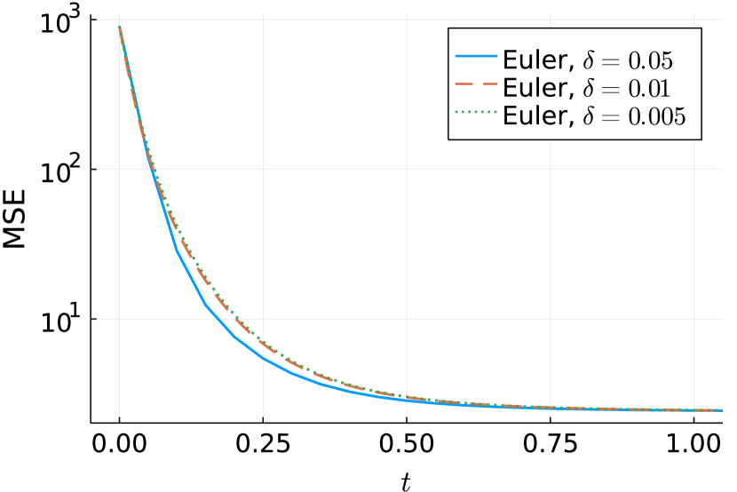
Figure 2: Evaluation on accuracy of the Euler method depending on step-size values, $(n,m,\sigma^{2},\eta,t_{\max},\kappa)=(8,8,1,0.5,3,158.29)$.

First, we verify a sufficient value for the step size $\delta$ to accurately simulate the ODE (6) because too large $\delta$ may lead to inaccurate behavior. Figure 2 shows MSE values for each choice of $\delta$. The system parameters were set to $(n,m,\sigma^{2},\eta)=(8,8,1,0.5)$. We set $t_{\max}=3$ and $\delta=0.05,0.01$, and $0.005$. We generated a single instance of the channel matrix $\bm{H}$, where each element follows an independent and identically distributed $\mathcal{CN}(0,1)$. All subsequent experiments generated $\bm{H}$ similarly. The condition number of the Gram matrix $\bm{H}^{\mathrm{H}}\bm{H}$ was $\kappa=158.29$. For the Monte Carlo simulation, pairs of $(\bm{s},\bm{w})$ and the corresponding received signal $\bm{y}$ were generated $1000$ times and then the arithmetic MSE, the estimate of MSE calculated from arithmetic mean of squared errors, was computed with the matrix $\bm{H}$ fixed. From Fig. 2, there is no visible difference between the MSE curves for $\delta=0.01$ and $\delta=0.005$, so that we set $\delta$ to be smaller than 0.01 in the following simulations.

We then compare the MSE obtained from (14) with the arithmetic MSE obtained for a single instance of the channel matrix $\bm{H}$ with $\kappa=164.17$. Fig. 3 shows the MSE values derived from (14), arithmetic MSE values of the Euler method, and asymptotic MSE values of the ODE-MMSE method. The system parameters were set to $(n,m,\sigma^{2},\eta)=(8,8,1,0.5)$. The horizontal line indicates the asymptotic MSE (20). We set $\delta=10^{-3}$ for the Euler method. The arithmetic MSE was calculated for 1000 trials using Monte Carlo simulation. The curve of the analytical formula is comparable to that of the Euler method with sufficient accuracy. We can see that the MSE value converges to the asymptotic MSE value. These results are consistent with the MSE analysis in Sect. IV-A where the MSE of the ODE-MMSE method can be described by the analytical formula (14), and the MSE value assymptotically converges to the value given in (20).

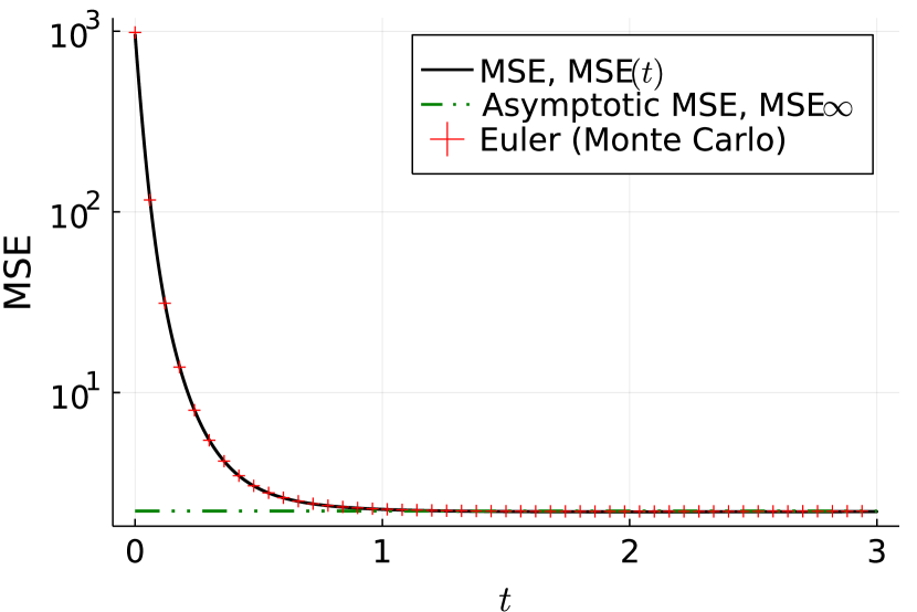
Figure 3: Comparison of MSE derived from analytical formula with the arithmetic MSE of the Euler method, $(n,m,\sigma^{2},\eta,\kappa)=(8,8,1,0.5,164.17)$.

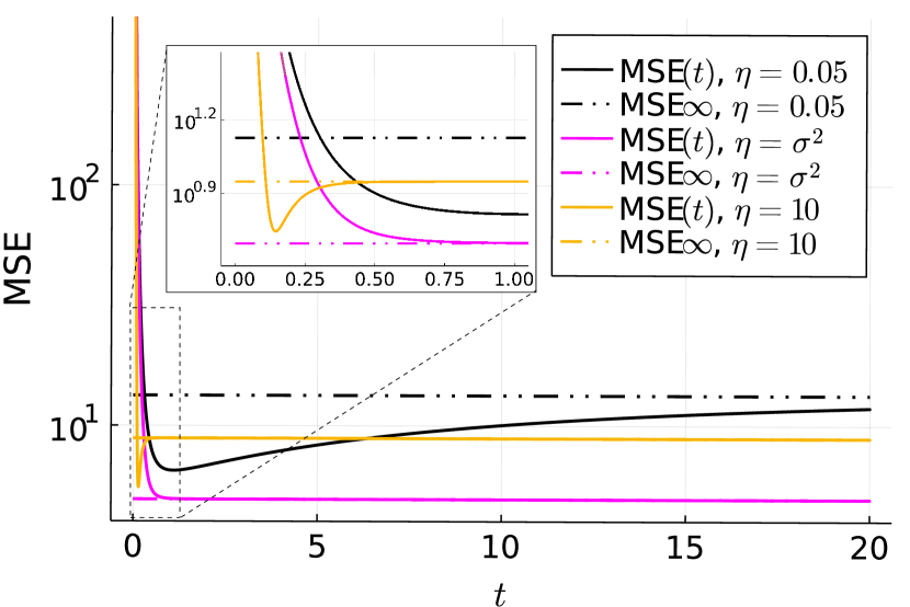
Figure 4: Comparison of MSE with different choices of the regularization parameter $\eta$, $(n,m,\sigma^{2},\kappa)=(32,32,1,3727.67)$.

We also evaluated the influence of regularization parameter $\eta$ on the convergence behavior of the ODE-MMSE method. Fig. 4 shows the MSE values obtained from (14) for different values of $\eta$: $\eta=0.05,\sigma^{2},10$. The system parameters were set to $(n,m,\sigma^{2})=(32,32,1)$. The condition number of the Gram matrix was $\kappa=3727.67$. With regard to the convergence rate, the MSE with $\eta=10$ decreases rapidly and that with $\eta=0.05$ is the slowest among the choices. This result is consistent with the interpretation of (14) where a larger $\eta$ accelerates the decay of the exponential terms. On the other hand, for the asymptotic MSE values, the value is the lowest when $\eta=\sigma^{2}$ and the choice $\eta=0.005$ leads to the highest value although the MSE is lower for $0.5<t<1$ than that for $\eta=10$. Therefore, the convergence behavior largely depends on the choice of regularization parameter $\eta$ and the superiority and inferiority of the MSE values can be switched depending on the time of interest.

V Time-dependent Regularization Parameter

This section introduces time-dependent control of the regularization parameter to improve the convergence property of the ODE-MMSE method.

V-A Derivation of MSE Formula

According to the theoretical and simulation results in the previous section, the regularization parameter $\eta$ significantly affects the convergence properties of ODE-MMSE method. Theorem 1 and Fig. 4 indicate that a larger $\eta$ yields faster convergence of the ODE-MMSE method but yields a worse MSE value than the MMSE estimation ($\mathrm{MSE}_{\infty}$ with $\eta=\sigma^{2}$). From these results, the adoption of time-dependent control of the regularization parameter $\eta$ is expected to hold both properties of faster convergence and a better asymptotic MSE value. In this section, we improve ODE-MMSE method to be more flexible by employing a time-dependent regularization parameter $\eta(t)$.

We consider an estimate of $\bm{s}$ that evolves according to the following ODE:

$$\frac{d\bm{x}(t)}{dt}=-(\bm{H}^{\mathrm{H}}\bm{H}+\eta(t)\bm{I})\bm{x}(t)+\bm{H}^{\mathrm{H}}\bm{y}.$$ (22)

The expression $\eta(t)$ implies that the regularization parameter can vary depending on the time $t$. The initial condition is the same as that in (6), i.e., $\bm{x}(0)=\bm{H}^{\mathrm{H}}\bm{y}$. We name the proposed signal detection based on ODE (22) ODE-MMSE with time-dependent regularization parameter (tODE-MMSE) method.

The ODE (22) can be solved using the variation of parameters method [19] because the matrix $\bm{A}(t):=\bm{H}^{\mathrm{H}}\bm{H}+\eta(t)\bm{I}$ is commutative.

Proposition 4

Estimate of the tODE-MMSE method at time $t\geq 0$ that follows the ODE (22) is given by

$$\bm{x}(t) =\exp{\left(-\bm{H}^{\mathrm{H}}\bm{H}t-\xi(t)\bm{I}\right)}$$

$$\ \cdot\left(\bm{I}+\int_{0}^{t}e^{\bm{H}^{\mathrm{H}}\bm{H}u+\xi(u)\bm{I}}du\right)\bm{H}^{\mathrm{H}}\bm{y},$$ (23)

where $\xi(T):=\int_{0}^{T}\eta(s)ds$.

Even in this case, the MSE formula for (23) can be derived in the same manner as in Sect. IV-A.

Theorem 2

The MSE for the tODE-MMSE method is given by

$$\mathrm{MSE}(t) =\sum_{i=1}^{n}\lambda_{i}(\lambda_{i}+\sigma^{2})\!\left(1\!+\!\int_{0}^{t}e^{\lambda_{i}u+\xi(u)}du\right)^{2}\!e^{-2(\lambda_{i}t+\xi(t))}$$

$$\ -2\sum_{i=1}^{n}\lambda_{i}\left(1+\int_{0}^{t}e^{\lambda_{i}u+\xi(u)}du\right)e^{-(\lambda_{i}t+\xi(t))}+n.$$ (24)

Proof: MSE can be derived using the same procedure as in Theorem 1 by employing the eigenvalue decomposition of the Gram matrix. Note that $\xi(t)$ is a scalar and that an integral in terms of a matrix is applied elementwise. The detailed derivation is shown in Appendix C. $\Box$

We obtain the result of Theorem 1 by setting $\eta(t)=\eta$. The analytical formula (24) has a complicated form, but, as with the ODE-MMSE method, the form of the time-dependent function $\eta(t)$ influences behavior of the estimation.

V-B Numerical Examples

We show numerical examples to confirm validity of the MSE formula (24) and to compare the convergence performance of the tODE-MMSE method with that of the ODE-MMSE method.

The integral $\xi(t)=\int_{0}^{t}\eta(s)ds$ is analytically tractable in certain cases. For convenience, we use the following parametric model for the function $\eta(t)$:

$$\eta(t)=\frac{1}{\alpha t+\epsilon}+\sigma^{2},$$ (25)

where $\alpha$ is a parameter and $\epsilon$ is a small number fixed at $10^{-8}$ in this paper. The integral can be calculated as $\xi(t)=1/\alpha\log\left((\alpha t+\epsilon)/\epsilon\right)+\sigma^{2}t.$ The shape of the function $\eta(t)$ is shown in Fig. 5, where $\sigma^{2}=1$ and $\alpha=10,100$. The function $\eta(t)$ first shows a higher value than $\sigma^{2}$ then converges to $\sigma^{2}$ at the limit $t\to\infty$. This formulation is derived from the results in Fig. 4, where the MSE decreases rapidly with larger $\eta$ and the asymptotic MSE becomes the lowest when $\eta=\sigma^{2}$.

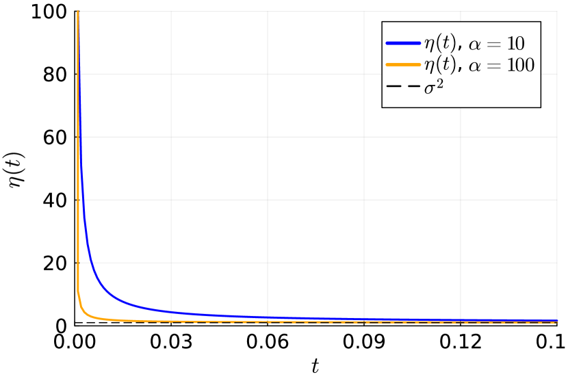
Figure 5: Example of $\eta(t)\ (\sigma^{2}=1,\alpha=10,100)$. The solid line is the function $\eta(t)$ (25) and the horizontal dash line is $\eta(t)=\sigma^{2}$.

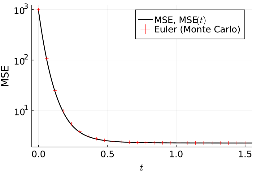
Figure 6: Comparison of MSE derived from analytical formula with the arithmetic MSE of Euler method, $(n,m,\sigma^{2},\alpha,\kappa)=(8,8,1,500,229.74)$.

We compare the MSE obtained from (24) with the arithmetic MSE obtained from Monte Carlo simulation under a single instance of the channel matrix $\bm{H}$. We employed the Euler method where $\eta$ in the equation (21) was replaced with $\eta(t_{N})$. Fig. 6 shows the MSE values at time $t$ of the methods. We used the tractable regularization function (25) with $\alpha=500$. The system parameters were set to $(n,m,\sigma^{2})=(8,8,1)$. The condition number of the Gram matrix was $\kappa=229.74$. The curve of the MSE obtained using (24) is comparable to that of the Euler method with sufficient accuracy. This result is consistent with the MSE analysis in Sect. V-A.

Finally, we present an example that uses the MSE formula (24) of tODE-MMSE method for improving the convergence properties and compare the performance with that of ODE-MMSE method. We have found in Fig. 4 that the performance of the proposed method largely depends on the choice of regularization parameter. It is expected that we can improve the convergence property by the tODE-MMSE method with an appropiate choice of the function $\eta(t)$. There are various possible indicators for evaluating the goodness of convergence performance. In this paper, we employed a functional

$$F(\xi(t)):=\int_{0}^{T}\mathrm{MSE}(t)dt$$

as the indicator. If a method has faster convergence and lower errors, the value of the functional decreases. In the following, we optimize the parameter by minimizing the functional value. Specifically, we employ a grid search to select the optimal parameter.

We set $\alpha=1,10,50,100$ as the parameter candidates. The system parameters were set to $(n,m,\sigma^{2})=(8,8,1)$ and $T=0.8$. The condition number of the Gram matrix was $\kappa=305.45$. Table I summarizes the evaluated values of $F(\xi(t))=F(\alpha)$. From the table, the value is found the lowest when $\alpha=10$. Fig. 7 shows the MSE of MMSE estimate $\mathrm{MSE}_{\mathrm{mmse}}$, the MSE values of ODE-MMSE method with $\eta=\sigma^{2}$, and those of tODE-MMSE method for different values of $\alpha$. From Fig. 7, all the MSE curves of tODE-MMSE method converge to the value of $\mathrm{MSE}_{\mathrm{mmse}}$ faster than the ODE-MMSE method. Furthermore, the method with $\alpha=10$, which has the lowest functional value in Table I, exhibited the fastest convergence. This indicates that an improved estimation method can be determined through a grid search using the functional value.

TABLE I: Values of functional $F(\alpha)$.

$\alpha$	$1$	$10$	$50$	$100$
$F(\alpha)$	$2.8963$	$2.5593$	$13.8035$	$19.5093$

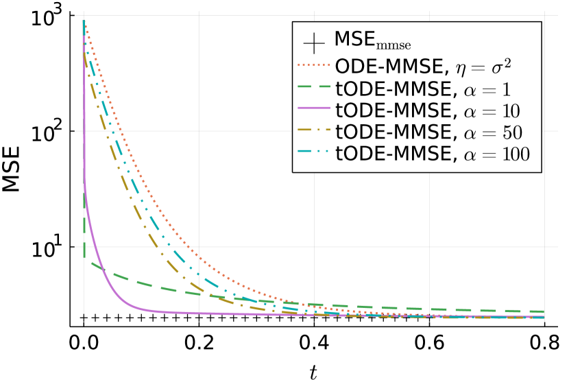
Figure 7: The MSE curves with different values of $\alpha$, $(n,m,\sigma^{2},\kappa)=(8,8,1,305.45)$.

VI Derivation of Discrete-time Algorithms

In this section, we present discrete-time MMSE estimation algorithms derived from continuous-time methods. This can be achieved by applying numerical methods to ODE.

VI-A Discretization of ODE

Let us derive discrete-time algorithms from ODE-MMSE method.

In the ODE-MMSE method for continuous-time MMSE estimation, the estimate of the transmitted signal evolves according to the ODE

$$\frac{d\bm{x}(t)}{dt}=-\nabla f(\bm{x})=-(\bm{H}^{\mathrm{H}}\bm{H}+\eta\bm{I})\bm{x}(t)+\bm{H}^{\mathrm{H}}\bm{y}.$$ (26)

The behavior of the estimate can be discretized and traced using numerical methods such as the well-known Euler method and Runge-Kutta method [19].

The explicit Euler method is the simplest numerical method. Applying the explicit Euler method to the ODE yields the following update equation, as discussed in Sect. IV-B:

$$\bm{x}^{[k]} =\bm{x}^{[k-1]}-\delta\nabla f(\bm{x}^{[k-1]})$$ (27)

$$=\bm{x}^{[k-1]}-\delta(\bm{H}^{\mathrm{H}}\bm{H}+\eta\bm{I})\bm{x}^{[k-1]}+\delta\bm{H}^{\mathrm{H}}\bm{y},$$ (28)

where $\delta$ is the step-size parameter. This is one of the discrete-time algorithms for MMSE estimation, which is summarized in Algorithm 1. The update equation has the same formulation as that of the conventional estimation method based on the standard gradient descent method [29]. It is known that the optimal step size in terms of the convergence rate depends on the maximum and minimum eigenvalues of the coefficient matrix. In particular, the optimal step size [30] in this case is

$$\delta=\frac{2}{\lambda_{1}+\lambda_{n}+2\eta}.$$ (29)

Algorithm 1 Euler method-based MMSE estimation

0:  Step-size parameter $\delta$, initial value $\bm{x}_{0}=\bm{H}^{\mathrm{H}}\bm{y}$

0:  Estimate $\bm{x}^{[J]}$

1:  for $k=1,\ldots,J$ do

2:     $\bm{x}^{[k]}=\bm{x}^{[k-1]}-\delta\left((\bm{H}^{\mathrm{H}}\bm{H}+\eta\bm{I})\bm{x}^{[k-1]}-\bm{H}^{\mathrm{H}}\bm{y}\right)$

3:  end for

Another famous and classical numerical method is the explicit 4th-stage (4th-order) Runge-Kutta method. The update equation is given by

$$\bm{x}^{[k]}=\bm{x}^{[k-1]}-\frac{\delta}{6}(\bm{c}_{1}+2\bm{c}_{2}+2\bm{c}_{3}+\bm{c}_{4}),$$ (30)

where $\bm{c}_{1}=\nabla f(\bm{x}^{[k-1]})$, $\bm{c}_{2}=\nabla f(\bm{x}^{[k-1]}+\delta\bm{c}_{1}/2)$, $\bm{c}_{3}=\nabla f(\bm{x}^{[k-1]}+\delta\bm{c}_{2}/2)$, and $\bm{c}_{4}=\nabla f(\bm{x}^{[k-1]}+\delta\bm{c}_{3})$. The process is summarized in Algorithm 2.

Algorithm 2 Runge-Kutta method-based MMSE estimation

0:  Step-size parameter $\delta$, initial value $\bm{x}_{0}=\bm{H}^{\mathrm{H}}\bm{y}$, gradient $\nabla f(\bm{x})=(\bm{H}^{\mathrm{H}}\bm{H}+\eta\bm{I})\bm{x}-\bm{H}^{\mathrm{H}}\bm{y}$

0:  Estimate $\bm{x}^{[J]}$

1:  for $k=1,\ldots,J$ do

2:     $\bm{c}_{1}=\nabla f(\bm{x}^{[k-1]})$

3:     $\bm{c}_{2}=\nabla f(\bm{x}^{[k-1]}+\frac{\delta}{2}\bm{c}_{1})$

4:     $\bm{c}_{3}=\nabla f(\bm{x}^{[k-1]}+\frac{\delta}{2}\bm{c}_{2})$

5:     $\bm{c}_{4}=\nabla f(\bm{x}^{[k-1]}+\delta\bm{c}_{3})$

6:     $\bm{x}^{[k]}=\bm{x}^{[k-1]}-\frac{\delta}{6}(\bm{c}_{1}+2\bm{c}_{2}+2\bm{c}_{3}+\bm{c}_{4})$

7:  end for

An example of the MSE performance of Euler method-based and 4th-stage Runge-Kutta method-based MMSE estimations is shown in Fig. 8. The condition number of the Gram matrix $\bm{H}^{\mathrm{H}}\bm{H}$ was $\kappa=12.02$. The system parameters were set to $(n,m,\sigma^{2},\eta)=(20,50,1,1)$. The arithmetic MSE was calculated for 1000 trials using Monte Carlo simulation. We used QPSK transmitted signal $\bm{s}$ for all the following Monte Carlo simulations. The MSE of the 4th-stage Runge-Kutta method-based algorithm decreases faster than that of the Euler method-based algorithm. However, the 4th-stage Runge-Kutta method-based algorithm includes four gradient calculations for $\bm{c}_{1},\bm{c}_{2},\bm{c}_{3},\bm{c}_{4}$ in each iteration, which accounts for the majority of the computational complexity. The computational cost is four times higher than that of the Euler method-based algorithm. This implies that there is no advantage as the discrete-time algorithm by considering the performance obtained with the same amount of computation.

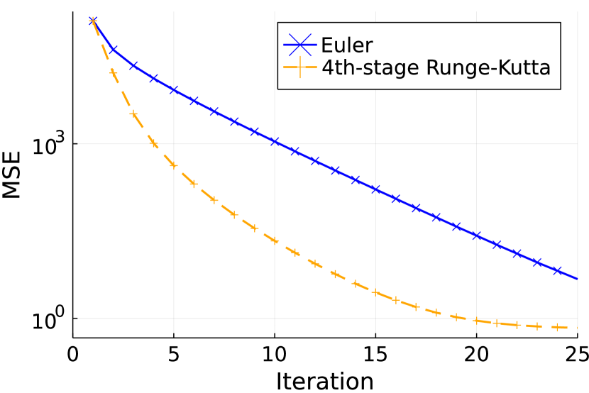
Figure 8: MSE curves of Euler method and Runge-Kutta method, $(n,m,\sigma^{2},\kappa)=(20,50,1,12.02)$.

More stable and computationally reasonable numerical methods for solving ODEs have long been explored [19], [31, 32, 33, 22, 34]. The meaning of more stable methods is that we can employ larger step-size parameter under guarantees of the stability and it leads a faster convergence of algorithms. For quadratic objective functions such as (4), Runge-Kutta-based method is proven to have higher stability by applying Chebyshev polynomials [35] to the update equation [33]. This procedure corresponds to the introduction of a flexible step size in the Runge-Kutta method.

The Runge-Kutta Chebyshev descent (RKCD) method [22] has both stability and computational tractability with a computational cost comparable to that of the explicit Euler method and its performance has been analyzed in recent years. RKCD method can achieve faster convergence than the standard gradient-based (Euler) method with comparable costs due to its high stability.

The RKCD method can be applied to the ODE for MMSE estimation (26). The algorithm includes a damping constant $\epsilon$ and the lower/upper bounds $\ell,L$ of the eigenvalues of $\bm{H}^{\mathrm{H}}\bm{H}$ or simply the lowest/highest eigenvalues $\lambda_{n}$, $\lambda_{1}$. The stability of the method is guaranteed by the damping constant. The other parameters $s,\omega_{0},\omega_{1},$ and $h$ are required to guarantee stability. The parameter $s$ can be regarded as the number of internal stages in Runge-Kutta method, $\omega_{0}$ determines the stability region, $\omega_{1}$ is required to satisfy the consistency, and $h$ is a step-size parameter. A reasonable choice of $\omega_{0}$ and $\omega_{1}$ [32] is known as

$$\omega_{0}:=1+\frac{\epsilon}{s^{2}},\ \omega_{1}:=\frac{T_{s}(\omega_{0})}{T_{s}^{\prime}(\omega_{0})},$$ (31)

where $T_{s}(z)$ is Chebyshev polynomial of the first kind with $j$ dimensional and is given by

$$T_{s}(\cos\theta)=\cos{(s\theta)}.$$ (32)

The parameters $s$ and $h$ can be chosen arbitrarily as long as the stability holds, and one choice guaranteeing the stability discussed in [22] is

$$s:=\left\lceil\sqrt{\frac{\left(-1+\frac{L}{\ell}\right)\epsilon}{2}}\right\rceil,$$ (33)

$$h:=\frac{\omega_{0}-1}{\omega_{1}(\ell+\eta)}.$$ (34)

An update equation fpr the RKCD method can be obtained by applying the Chebyshev polynomial to the update equation of $s$-stage Runge-Kutta method and by using the recurrence relation of the Chebyshev polynomial

$$T_{s+1}(z)=2zT_{s}(z)-T_{s-1}(z).$$ (35)

The specific update is given by

$$\bm{x}^{[k]} =-h\mu_{j}\left((\bm{H}^{\mathrm{H}}\bm{H}+\eta\bm{I})\bm{x}^{[k-1]}-\bm{H}^{\mathrm{H}}\bm{y}\right)$$

$$\quad\quad+\nu_{j}\bm{x}^{[k-1]}-(\nu_{j}-1)\bm{x}^{[k-2]},$$ (36)

where $j=\mod{(k-1,s)}+1$,

$$\mu_{j}:=\frac{2\omega_{1}T_{j-1}(\omega_{0})}{T_{j}(\omega_{0})},\ \nu_{j}:=\frac{2\omega_{0}T_{j-1}(\omega_{0})}{T_{j}(\omega_{0})}.$$ (37)

The function $\mathrm{mod}(k,s)$ means the remainder of $k/s$. The step-size parameters for the method are represented using $\mu_{j}$ and $\nu_{j}$, which is discussed in a later section.

Algorithm 3 summarizes the detailed process of RKCD method for MMSE estimation. Computational complexity of this method is dominated by matrix-vector product. It is comparable to the Euler method for MMSE estimation.

Algorithm 3 RKCD method-based MMSE estimation

0:  Damping constant $\epsilon$, lower $\ell$ and upper bound $L$ for eigenvalues of $\bm{H}^{\mathrm{H}}\bm{H}$, initial value $\bm{x}_{0}=\bm{H}^{\mathrm{H}}\bm{y}$

0:  Estimate $\bm{x}^{[J]}$

1:  Set parameters $s$ and $h$ or use (33) and (34)

2:  Set parameters $\omega_{0}=1+\frac{\epsilon}{s^{2}}$ and $\omega_{1}=\frac{T_{s}(\omega_{0})}{T_{s}^{\prime}(\omega_{0})}$

3:  $\bm{x}^{[0]}=\bm{x}_{0}$

4:  for $k=1,\ldots,J$ do

5:     if $\mod{(k,s)}==1$ then

6:        $\bm{x}^{[k]}=\bm{x}^{[k-1]}-\frac{h\omega_{1}}{\omega_{0}}\left((\bm{H}^{\mathrm{H}}\bm{H}+\eta\bm{I})\bm{x}^{[k-1]}-\bm{H}^{\mathrm{H}}\bm{y}\right)$

7:     else

8:        $j=\mod{(k-1,s)}+1$

9:        $\mu_{j}=\frac{2\omega_{1}T_{j-1}(\omega_{0})}{T_{j}(\omega_{0})}$

10:        $\nu_{j}=\frac{2\omega_{0}T_{j-1}(\omega_{0})}{T_{j}(\omega_{0})}$

11:        $\bm{x}^{[k]}=-h\mu_{j}\left((\bm{H}^{\mathrm{H}}\bm{H}+\eta\bm{I})\bm{x}^{[k-1]}-\bm{H}^{\mathrm{H}}\bm{y}\right)+\nu_{j}\bm{x}^{[k-1]}-(\nu_{j}-1)\bm{x}^{[k-2]}$

12:     end if

13:  end for

It is possible to construct novel algorithms for MMSE estimation by adopting the perspective of numerical methods, which is different from conventional discrete-time algorithms such as [21]. In other words, we can also obtain benefits on digital-domain signal processing through the expression as an ODE.

VI-B Numerical Examples

In this section, we evaluate the estimation performance of the discrete-time MMSE estimation algorithms obtained using numerical methods. The performance is compared with that of a conventional MMSE estimation algorithm [21] based on the Jacobi [36] and successive over-relaxation (SOR) methods [37]. We call the method in this paper the Jacobi SOR algorithm. The Jacobi SOR algorithm has been reported to achieve fast convergence in well-conditioned channels with $\mathcal{O}(n^{2})$ complexity and have high parallelism, which are the same characteristics as the Euler and RKCD method-based detection algorithms.

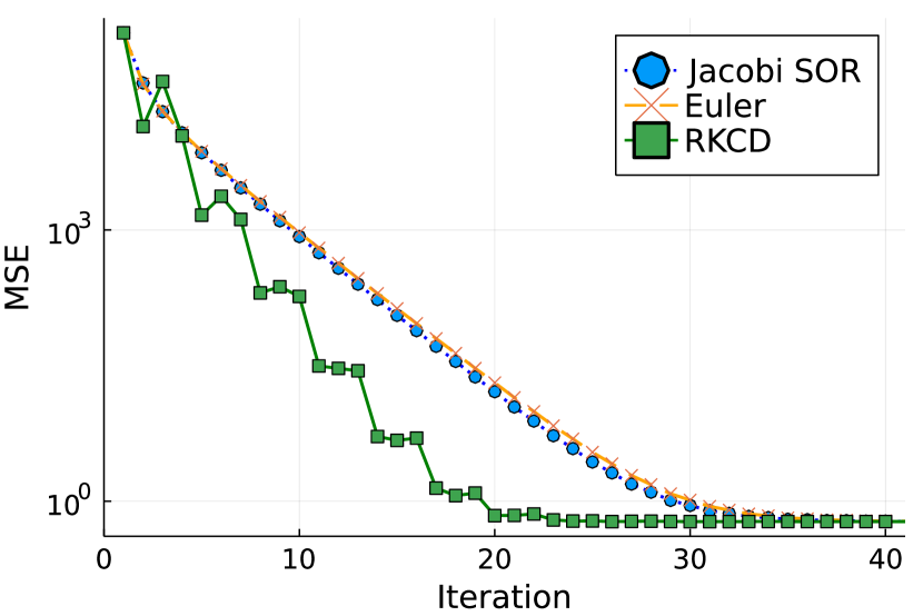
Figure 9: MSE comparison of discrete-time MMSE estimation method, Jacobi SOR method, Euler method, and RKCD method, $(n,m,\sigma^{2},\kappa)=(20,50,1,11.38)$.

Figure 9 shows the performance of the Euler method-, RKCD method-based algorithms, and conventional Jacobi SOR algorithm. The step-size parameter $\delta$ in the Euler method was set to the optimal one (29). For the RKCD method, the damping constant was set to $\epsilon=1.17$, the parameters $s$ and $h$ were set as in (33) and (34), respectively, and we employed accurate eigenvalues $\lambda_{1}$ and $\lambda_{n}$ as the lower bound $\ell$ and upper bound $L$, respectively. In this case, the parameter $s$ was 3. The condition number of the Gram matrix $\bm{H}^{\mathrm{H}}\bm{H}$ was $\kappa=11.38$. The system parameters were set to $(n,m,\sigma^{2},\eta)=(20,50,1,1)$. The arithmetic MSE was calculated for 1000 trials using Monte Carlo simulation. From Fig. 9, the Euler method-based and Jacobi SOR algorithms show comparable performance. The RKCD method-based algorithms achieves lower error and the suitable choices (33) and (34) yield the best estimation performance.

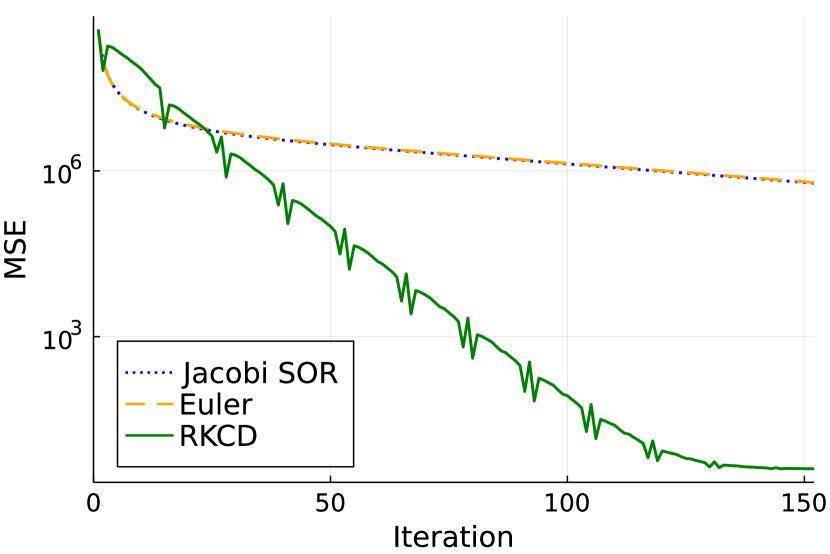
Figure 10: MSE comparison of discrete-time MMSE estimation method, Jacobi SOR method, Euler method, and RKCD method, $(n,m,\sigma^{2},\kappa)=(400,500,1,305.86)$.

MSE performance of another system is shown in Fig. 10. The system parameters were set to $(n,m,\sigma^{2},\eta)=(400,500,1,1)$. The condition number of the Gram matrix $\bm{H}^{\mathrm{H}}\bm{H}$ was $\kappa=305.86$. The arithmetic MSE was calculated for 100 trials using Monte Carlo simulation. In this case, the parameter $s$ of the RKCD method-based algorithm was 14. The settings of the other parameters were the same as those in Fig. 9. The slopes of the curves of the Jacobi SOR and Euler methods are large up to 10 iterations, but then decrease immediately. On the other hand, the RKCD method maintained a large slope and it leads to a large performance gap compared with other methods. The results show that RKCD method performs better also in the case of system with a large condition number.

As the numerical results show, it is possible to create algorithms that exhibit performance not achievable using conventional discrete-time algorithms by constructing an ODE to solve the problem of interest and discretizing the ODE with ingenious step-size parameters.

VII Benefits of ODE on Discrete-time Algorithms

This section confirms the hypotheses that theoretical analysis of continuous-time detection methods can be valuable for discrete-time algorithms. In Sect. VI, we provide a theoretical analysis of discrete-time MMSE detection algorithms. Moreover, we apply the time-dependent regularization parameter to the discrete-time algorithms that is optimized for continuous-time methods.

VII-A MSE Analysis for Discrete-time Algorithms

There is considerable interest in understanding the relationship between performance and runtime of discrete algorithms. For this purpose, it is desirable to clarify MSE performance in each iteration of the algorithms but the performance cannot always be traced analytically, as discussed in Sect. IV-A. However, the use of ODE may facilitate this. Solution of continuous-time methods represented by ODE can be numerically traced using numerical methods discretized with sufficient accuracy. In this case, the MSE of the discrete-time numerical methods should agree with the result of MSE analysis for the continuous-time method. Therefore, the MSE analysis in continuous-time methods also allows us to analyze the performance of discrete-time algorithms obtained by discretizing the ODE. In other words, the MSE performance of Algorithms 1–3 obtained from ODE (26) can be described using the MSE formula (14). Note that the above discussion does not hold if one uses a numerical method with insufficient accuracy, i.e., with a large step-size parameter.

For the Euler method-based MMSE estimation (Algorithm 1), the estimate $\bm{x}^{[k]}$ at $k$th iteration corresponds to the estimate at the time $t_{k}=\delta k$. Therefore, the MSE of the method at the $k$th iteration, defined as $\mathrm{MSE}_{\mathrm{Euler}}[k]$, is given by

$$\mathrm{MSE}_{\mathrm{Euler}}[k]\simeq\mathrm{MSE}(\delta k)$$ (38)

by using the MSE formula (14).

A similar argument also holds for the RKCD method-based MMSE estimation (Algorithm 3). The corresponding time $T_{k}$ of the estimate at $k$ th iteration ($k=1,2,\ldots$) can be described recursively [31] as

$$T_{k}\!=\!\begin{cases}\tilde{t}_{k}\!+\!\frac{h\omega_{1}}{\omega_{0}},&\mathrm{if}\mod(k,s)=1,\\ \tilde{t}_{k}\!+\!\nu_{k}T_{k-1}\!+\!(1\!-\!\nu_{k})T_{k-2}\!+\!h\mu_{k},&\mathrm{otherwise},\end{cases}$$ (39)

where $\tilde{t}_{0}=0$ and $\tilde{t}_{k}=\tilde{t}_{k-1}+T_{k}$ if $\mod(k,s)=0$ otherwise, $\tilde{t}_{k}=\tilde{t}_{k-1}$. This implies that the step-size parameters of RKCD method depend on the iteration index. The MSE value of the method, $\mathrm{MSE}_{\mathrm{RKCD}}[k]$, is given by

$$\mathrm{MSE}_{\mathrm{RKCD}}[k]\simeq\mathrm{MSE}(T_{k}).$$ (40)

We present a numerical example of the behavior of the discrete-time algorithm. Figure 11 shows the MSE values obtained from the MSE formula (14) and arithmetic MSE values obtained using the RKCD method-based estimation method. The system parameters were set to $(n,m,\sigma^{2})=(20,50,1)$ and the regularization parameter was $\eta=1$. The condition number of the Gram matrix was $\kappa=13.93$ in this case. The parameter $s$ for the RKCD method was determined by (33) and $h$ was set to $h=0.03185$. We performed 100 trials to calculate the arithmetic MSE values, which are displayed as markers in the figure. The standard deviation of the squared error is shown as error bars. From Fig. 11, the arithmetic MSE values are close to the theoretical values. In other words, the performance behavior of the algorithm can be well described using the MSE formula.

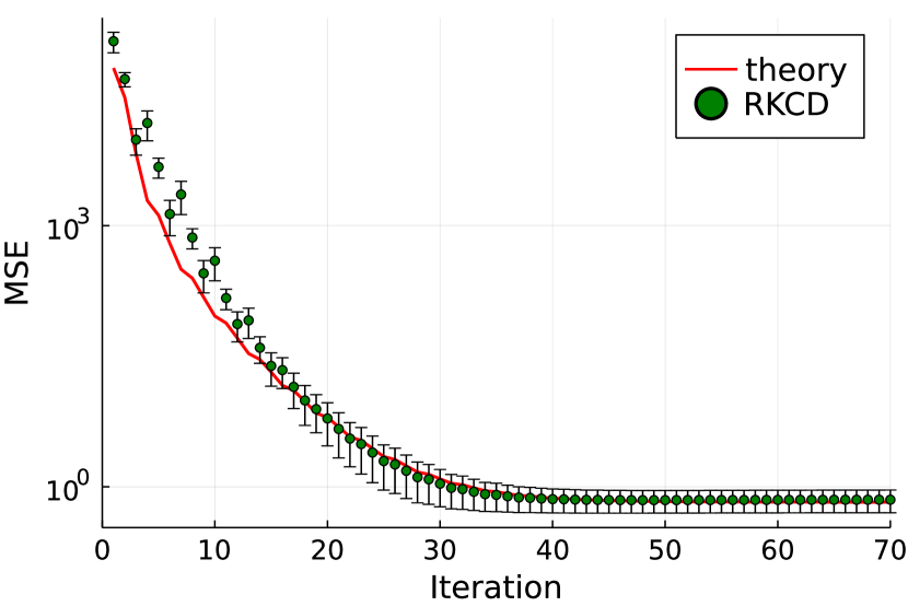
Figure 11: MSE obtained by MSE formula and arithmetic MSE of RKCD, $(n,m,\sigma^{2},\kappa)=(20,50,1,13.93)$.

VII-B Time-dependent Regularization Parameter

In Sect. V, we have introduced the time-dependent scheduling of the regularization parameter into the continuous-time MMSE detection method. The scheduling has been optimized by using the MSE formula for the tODE-MMSE method, resulting in improved convergence performance. Optimized scheduling for continuous-time methods can be valuable also for discrete-time algorithms. In this section, we apply the optimized scheduling of the regularization parameter to discrete-time algorithms and then evaluate the convergence performance.

The implementation of time-dependent scheduling is simple where fixed regularization parameter $\eta$ in the algorithms are just replaced with a time-dependent $\eta(t)$ corresponding to discrete time. For the Euler method-based MMSE estimation, the fixed regularization parameter $\eta$ in line 2 of Algorithm 1 is replaced with the time-dependent $\eta(t_{k})=\eta(\delta k)$. For the RKCD method-based MMSE estimation, $\eta$s in lines 7 and 12 of Algorithm 3 are replaced by $\eta(T_{k})=\eta(\tilde{t}_{k}+h\omega_{1}/\omega_{0})$ and $\eta(T_{k})=\eta(\tilde{t}_{k}+\nu_{j}T_{k-1}+(1-\nu_{j})T_{k-2}+h\mu_{j})$, respectively.

The convergence performance is evaluated using numerical simulations. Figure 12 shows the arithmetic MSE values of the Euler method- and RKCD method-based estimation methods with fixed and time-dependent regularization parameters. Similar system parameters and the same channel matrix $\bm{H}$ as in Fig. 7 were used. The hyperparameter $\alpha$ included in the function $\eta(t)$ (25) was set to $\alpha=10$, which is the best choice from the theoretical results in Fig. 7. The step-size parameter $\delta$ for the Euler method and the parameter $h$ for the RKCD method were set to $\delta=0.005$ and $h=0.1075$, respectively. The parameter $s$ was determined by (33). From Fig. 12, the convergence performance is improved by adoption of the time-dependent regularization parameter for both cases. Therefore, optimizing scheduling of the regularization parameters is also effective for discrete-time algorithms, leading to improved performance. This suggests that the choice of regularization parameter can be decoupled from the choice of discretization method and step-size parameter in the discrete-time algorithm. As a result, the optimal scheduling can be applied to various algorithms.

Figure 12: MSE of Euler method and RKCD method with fixed $\eta$ and time-dependent $\eta(t)$, $(n,m,\sigma^{2},\eta,\kappa)=(8,8,1,1,305.45)$.

VIII Conclusions

We have explored continuous-time MMSE signal detection methods for MIMO systems as a potential solution to computational load issues in future wireless communication systems. We described the continuous-time estimation as an ODE and proposed the ODE-MMSE method. The analytical formula for the MSE was derived by using eigenvalue decomposition of the Gram matrix of the channel matrix. The simulation results showed the significant influence of the choice of the parameter $\eta$ on convergence performance. We also extended the ODE-MMSE method by introducing time-dependent parameter $\eta(t)$ and proposed the tODE-MMSE method. The MSE formula was derived also for the tODE-MMSE method. We then optimized the scheduling of $\eta(t)$ and we have through computer simulations shown that it improves the convergence performance.

Analog signal processing has excellent potential for improving computational efficiency and overcoming many of the limitations of traditional digital signal processing. Theoretical analysis of continuous-time signal detection method presented in this paper is expected to render analog computation a more realistic technology for next-generation communication systems. The findings of this study can inspire further research in the development of analog devices for signal processing.

As a further development of this study, we derived the discrete-time MMSE estimation algorithms by discretizing the ODE using numerical methods such as the Euler and Runge-Kutta Chebyshev descent methods. These algorithms can adopt the consideration of numerical stability and flexible selection of step-size parameters. The Runge-Kutta Chebyshev descent method-based detection algorithm achieves better convergence performance than the other methods without any additional computational costs. Theoretical analysis of continuous-time methods is beneficial also to the discrete-time algorithms. The MSE of the algorithms has become analytically tractable using the MSE formula for the ODE-MMSE method. Optimized scheduling of regularization parameters obtained from theoretical results of the tODE-MMSE method can be applied to discrete-time algorithms and yields improved convergence performance.

These advantages reveal that continuous-time signal processing and its analysis have the potential to be a new construction methodology for discrete-time algorithms. The approach proposed in this study can lead to the development of more efficient and accurate discrete-time signal processing algorithms and a deeper understanding of the fundamental principles of signal processing, which can have a wide range of practical applications.

Appendix A Derivation of Theorem 1

The matrix $\bm{Q}(t)$ is given by (8). By applying eigenvalue decomposition to $(\bm{H}^{\mathrm{H}}\bm{H}+\eta\bm{I})^{-1}$ and $\exp{(-(\bm{H}^{\mathrm{H}}\bm{H}+\eta\bm{I})t)}$, the matrix $\bm{Q}(t)$ can be expanded as

$$\bm{Q}(t) =\bm{U}\Bigl{(}\mathrm{diag}[e^{-(\lambda_{1}+\eta)t},\ldots,e^{-(\lambda_{n}+\eta)t}]$$

$$\quad\cdot\mathrm{diag}\Bigl{[}1-\frac{1}{\lambda_{1}+\eta},\ldots,1-\frac{1}{\lambda_{n}+\eta}\Bigr{]}$$

$$\quad+\mathrm{diag}\Bigl{[}\frac{1}{\lambda_{1}+\eta},\ldots,\frac{1}{\lambda_{n}+\eta}\Bigr{]}\Bigr{)}\bm{U}^{\mathrm{H}}\bm{H}$$

$$=\bm{U}\mathrm{diag}\Bigl{[}\frac{q(\lambda_{1})}{\lambda_{1}+\eta},\ldots,\frac{q(\lambda_{n})}{\lambda_{n}+\eta}\Bigr{]}\bm{U}^{\mathrm{H}}\bm{H},$$ (41)

where $q(\lambda_{i}):=e^{-(\lambda_{i}+\eta)t}(\lambda_{i}+\eta-1)+1$. The term (17) can be calculated by using this as

$$\mathrm{Tr}[\bm{Q}(t)^{\mathrm{H}}\bm{Q}(t)]$$

$$=\bm{U}\mathrm{diag}\Bigl{[}\frac{q(\lambda_{1})}{\lambda_{1}+\eta},\ldots,\frac{q(\lambda_{n})}{\lambda_{n}+\eta}\Bigr{]}\bm{U}^{\mathrm{H}}\bm{H}^{\mathrm{H}}\bm{H}$$

$$\quad\cdot\bm{U}\mathrm{diag}\Bigl{[}\frac{q(\lambda_{1})}{\lambda_{1}+\eta},\ldots,\frac{q(\lambda_{n})}{\lambda_{n}+\eta}\Bigr{]}\bm{U}^{\mathrm{H}}$$ (42)

$$=\mathrm{Tr}\left[\mathrm{diag}\left[\left(\frac{q(\lambda_{1})}{\lambda_{1}+\eta}\right)^{2}\lambda_{1},\ldots,\left(\frac{q(\lambda_{n})}{\lambda_{n}+\eta}\right)^{2}\lambda_{n}\right]\right]$$ (43)

$$=\sum_{i=1}^{n}\frac{\lambda_{i}\left(q(\lambda_{i})\right)^{2}}{(\lambda_{i}+\eta)^{2}}.$$ (44)

The term (18) can be also expanded as follows:

$$\mathrm{Tr}\left[(\bm{Q}(t)\bm{H}-\bm{I})^{\mathrm{H}}(\bm{Q}(t)\bm{H}-\bm{I})\right]$$ (45)

$$=\mathrm{Tr}\Biggl{[}\mathrm{diag}\Biggl{[}\left(\frac{q(\lambda_{1})\lambda_{1}}{\lambda_{1}+\eta}-1\right)^{2},\ldots,\left(\frac{q(\lambda_{n})\lambda_{n}}{\lambda_{n}+\eta}-1\right)\Biggr{]}\Biggr{]}$$ (46)

$$=\sum_{i=1}^{n}\frac{\left(\lambda_{i}q(\lambda_{i})-(\lambda_{i}+\eta)\right)^{2}}{(\lambda_{i}+\eta)^{2}}.$$ (47)

By substituting them into (15),

$$\mathrm{MSE}(t)$$

$$=\sum_{i=1}^{n}\frac{\left(\lambda_{i}q(\lambda_{i})-(\lambda_{i}+\eta)\right)^{2}}{(\lambda_{i}+\eta)^{2}}+\sigma^{2}\sum_{i=1}^{n}\frac{\lambda_{i}\left(q(\lambda_{i})\right)^{2}}{(\lambda_{i}+\eta)^{2}}$$ (48)

$$=\sum_{i=1}^{n}\frac{\lambda_{i}(\lambda_{i}+\eta-1)^{2}(\lambda_{i}+\sigma^{2})e^{-2(\lambda_{i}+\eta)t}}{(\lambda_{i}+\eta)^{2}}$$

$$\ -\sum_{i=1}^{n}\frac{2\lambda_{i}(\lambda_{i}+\eta-1)(\eta-\sigma^{2})e^{-(\lambda_{i}+\eta)t}}{(\lambda_{i}+\eta)^{2}}$$

$$\ +\sum_{i=1}^{n}\frac{\eta^{2}+\sigma^{2}\lambda_{i}}{(\lambda_{i}+\eta)^{2}}.$$ (49)

Appendix B Derivation of Lemma 1

The MSE of MMSE estimation is

$$\mathrm{MSE}_{\mathrm{mmse}}=\mathbb{E}[\|\hat{\bm{s}}-\bm{s}\|^{2}].$$ (50)

By substituting (3) into the definition,

$$\mathrm{MSE}_{\mathrm{mmse}}$$

$$=\mathbb{E}[\|\left(\bm{H}^{\mathrm{H}}\bm{H}+\sigma^{2}\bm{I}\right)^{-1}\bm{H}^{\mathrm{H}}(\bm{Hs}+\bm{w})-\bm{s}\|^{2}]$$ (51)

$$=\mathbb{E}\Biggl{[}\Bigl{\|}\left(\left(\bm{H}^{\mathrm{H}}\bm{H}+\sigma^{2}\bm{I}\right)^{-1}\bm{H}^{\mathrm{H}}\bm{H}-\bm{I}\right)\bm{s}$$

$$\ +\left(\bm{H}^{\mathrm{H}}\bm{H}+\sigma^{2}\bm{I}\right)^{-1}\bm{H}^{\mathrm{H}}\bm{w}\Bigr{\|}^{2}\Biggr{]}$$ (52)

$$=\mathrm{Tr}\Bigl{[}\left(\left(\bm{H}^{\mathrm{H}}\bm{H}+\sigma^{2}\bm{I}\right)^{-1}\bm{H}^{\mathrm{H}}\bm{H}-\bm{I}\right)^{\mathrm{H}}$$

$$\quad\cdot\left(\left(\bm{H}^{\mathrm{H}}\bm{H}+\sigma^{2}\bm{I}\right)^{-1}\bm{H}^{\mathrm{H}}\bm{H}-\bm{I}\right)\Bigr{]}$$

$$\ +\sigma^{2}\mathrm{Tr}\Bigl{[}\left(\left(\bm{H}^{\mathrm{H}}\bm{H}+\sigma^{2}\bm{I}\right)^{-1}\bm{H}^{\mathrm{H}}\right)^{\mathrm{H}}$$

$$\quad\cdot\left(\left(\bm{H}^{\mathrm{H}}\bm{H}+\sigma^{2}\bm{I}\right)^{-1}\bm{H}^{\mathrm{H}}\right)\Bigr{]},$$ (53)

where the second moments are $\mathbb{E}[\bm{ss}^{\mathrm{H}}]=\bm{I}$ and $\mathbb{E}[\bm{ww}^{\mathrm{H}}]=\sigma^{2}\bm{I}$. By applying eigenvalue decomposition to $\left(\bm{H}^{\mathrm{H}}\bm{H}+\sigma^{2}\bm{I}\right)^{-1}$ and $\bm{H}^{\mathrm{H}}\bm{H}$,

$$\mathrm{MSE}_{\mathrm{mmse}}$$

$$=\sum_{i=1}^{n}\left(\frac{\lambda_{i}}{\lambda_{i}+\sigma^{2}}-1\right)^{2}+\sigma^{2}\sum_{i=1}^{n}\left(\frac{\lambda_{i}}{(\lambda_{i}+\sigma^{2})^{2}}\right)$$ (54)

$$=\sum_{i=1}^{n}\frac{\sigma^{2}}{\lambda_{i}+\sigma^{2}}.$$ (55)

Appendix C Derivation of Theorem 2

The matrix integral in (23) can be decomposed as

$$\int_{0}^{t}e^{\bm{H}^{\mathrm{H}}\bm{H}u+\xi(u)\bm{I}}du$$

$$=\bm{U}\mathrm{diag}\left[\int_{0}^{t}e^{\lambda_{1}u+\xi(u)}du,\ldots,\int_{0}^{t}e^{\lambda_{n}u+\xi(u)}du\right]\bm{U}^{\mathrm{H}}.$$ (56)

By using this, the matrix included in (23) is also decomposed as

$$\exp{\left(-\bm{H}^{\mathrm{H}}\bm{H}t-\xi(t)\bm{I}\right)}\left(\bm{I}+\int_{0}^{t}e^{\bm{H}^{\mathrm{H}}\bm{H}u+\xi(u)\bm{I}}du\right)$$

$$=\bm{U}\Bigl{(}\mathrm{diag}\Bigl{[}e^{-(\lambda_{1}t+\xi(t))}\left(1+\int_{0}^{t}e^{\lambda_{1}u+\xi(u)}du\right),\ldots,$$

$$\quad e^{-(\lambda_{n}t+\xi(t))}\left(1+\int_{0}^{t}e^{\lambda_{n}u+\xi(u)}du\right)\Bigr{]}\Bigr{)}\bm{U}^{\mathrm{H}}.$$ (57)

Applying this to the definition of MSE leads to the analytical formula in the same way as Theorem 1.

Ayano Nakai-Kasai received the bachelor’s degree in engineering, the master’s degree in informatics, and Ph.D. degree in informatics from Kyoto University, Kyoto, Japan, in 2016, 2018, and 2021, respectively. She is currently an Assistant Professor at Graduate School of Engineering, Nagoya Institute of Technology. Her research interests include signal processing, wireless communication, and machine learning. She received the Young Researchers’ Award from the Institute of Electronics, Information and Communication Engineers in 2018 and APSIPA ASC 2019 Best Special Session Paper Nomination Award. She is a member of IEEE and IEICE.

Tadashi Wadayama (M’96) was born in Kyoto, Japan, on May 9,1968. He received the B.E., the M.E., and the D.E. degrees from Kyoto Institute of Technology in 1991, 1993 and 1997, respectively. On 1995, he started to work with Faculty of Computer Science and System Engineering, Okayama Prefectural University as a research associate. From April 1999 to March 2000, he stayed in Institute of Experimental Mathematics, Essen University (Germany) as a visiting researcher. On 2004, he moved to Nagoya Institute of Technology as an associate professor. Since 2010, he has been a full professor of Nagoya Institute of Technology. His research interests are in coding theory, information theory, and signal processing for wireless communications. He is a member of IEEE and a senior member of IEICE.

References

- [1] A. Nakai-Kasai and T. Wadayama, “MMSE signal detection for MIMO systems based on ordinary differential equation,” IEEE Global Communications Conference (GLOBECOM 2022), Rio de Janeiro, Brazil and virtual conference, Dec. 2022.
- [2] E. C. Strinati, D. Belot, A. Falempin, and J.-B. Doré, “Toward 6G: From new hardware design to wireless semantic and goal-oriented communication paradigms,” in Proc. ESSCIRC, Grenoble, France, Sept. 2021, pp. 275–282.
- [3] K. Li, R. Sharan, Y. Chen, T. Goldstein, J. R. Cavallaro, and C. Studer, “Decentralized baseband processing for massive MU-MIMO systems,” IEEE J. Emerg. Sel. top. Circuits Syst., vol. 7, no. 4, pp. 491–507, Dec. 2017.
- [4] E. Björnson, J. Hoydis, and L. Sanguinetti, “Massive MIMO networks: Spectral, energy, and hardware efficiency,” Found. Signal. Process. Commun. Netw., vol. 11, no. 3–4, pp. 154–655, Nov. 2017.
- [5] S. Chetan, J. Manikandan, V. Lekshmi, and S. Sudhakar, “Hardware implementation of floating point matrix inversion modules on FPGAs,” in Proc. ICM, Aqaba, Jordan, Dec. 2020, pp. 1–4.
- [6] T. Wadayama and A. Nakai-Kasai, “Continuous-time noisy average consensus system as Gaussian multiple access channel,” IEEE International Symposium on Information Theory (ISIT2022), Jun.–Jul. 2022.
- [7] T. Wadayama and A. Nakai-Kasai, “Ordinary differential equation-based sparse signal recovery,” International Symposium on Information Theory and Its Applications (ISITA2022), pp. 14–18, Oct. 2022.
- [8] J. Welser, J. W. Pitera, C. Goldberg, “Future computing hardware for AI,” in Proc. IEDM, San Francisco, CA, USA, Dec. 2018.
- [9] W. Haensch, T. Gokmen, and R. Puri, “The next generation of deep learning hardware: Analog computing,” Proc. IEEE, vol. 107, no. 1, pp. 108–122, Jan. 2019.
- [10] E. A. Cartier, W. Kim, N. Gong et al., “Reliability challenges with materials for analog computing,” in Proc. IRPS, Monterey, CA, USA, Mar.–Apr. 2019.
- [11] M. Paliy, S. Strangio, P. Ruiu, T. Rizzo, and G. Iannaccone, “Analog vector-matrix multiplier based on programmable current mirrors for neural network integrated circuits,” IEEE Access, vol. 8, pp. 203525–203537, 2020.
- [12] F. Ashtiani, A. J. Geers, and F. Aflatouni, “An on-chip photonic deep neural network for image classification,” Nature, vol. 606, no. 7914, pp. 501–506, Jun. 2022.
- [13] X. Lin, Y. Rivenson, N. T. Yardimci, M. Veli, Y. Luo, M. Jarrahi, and A. Ozcan, “All-optical machine learning using diffractive deep neural networks,” Science, vol. 361, no. 6406, pp. 1004–1008, Jul. 2018.
- [14] H. Zhang, M. Gu, X. D. Jiang et al., “An optical neural chip for implementing complex-valued neural network,” Nat. Commun., vol. 12, no. 457, pp. 1–11, Jan. 2021.
- [15] S. Abdollahramezani, O. Hemmatyar, and A. Adibi, “Meta-optics for spatial optical analog computing,” Nanophotonics, vol. 9, no. 13, pp. 4075–4095, Sept. 2020.
- [16] J. Capmany and D. Pérez, Programmable Integrated Photonics, Oxford University Press, 2020.
- [17] U. Helmke and J. B. Moore, Optimization and Dynamical Systems. Springer London, Mar. 1996.
- [18] R. T. Q. Chen, Y. Rubanova, J. Bettencourt, and D. K. Duvenaud, “Neural ordinary differential equaitons,” in Proc. NeurIPS, Montréal, Canada, Dec. 2018, pp. 1–13.
- [19] G. Teschl, Ordinary Differential Equations and Dynamical Systems, American Mathematical Soc., 2012.
- [20] L. Dai, X. Gao, X. Su, S. Han, C.-L. I, and Z. Wang, “Low-complexity soft-output signal detection based on Gauss–Seidel method for uplink multiuser large-scale MIMO systems,” IEEE Trans. Veh. Technol., vol. 64, no. 10, pp. 4839–4845, Oct. 2015.
- [21] A. Naceur, “Damped Jacobi methods based on two different matrices for signal detection in massive MIMO uplink,” J. Microw. Optoelectron. Electromagn. Appl., vol. 20, no. 1, pp. 92–104, Mar. 2021.
- [22] A. Eftekhari, B. Vandereycken, G. Vilmart, and K. C. Zygalakis, “Explicit stabilised gradient descent for faster strongly convex optimisation,” BIT, vol. 61, no. 1, pp. 119–139, Mar. 2021.
- [23] K. Li, O. Castañeda, C. Jeon, J. R. Cavallaro, C. Studer, “Decentralized coordinate-descent data detection and precoding for massive MU-MIMO,” in Proc. ISCAS, Sapporo, Japan, May 2019.
- [24] S. H. Strogatz, “Nonlinear dynamics and chaos: with applications to physics, biology chemistry and engineering,” Addison Wesley, 1994.
- [25] Y. Hama and H. Ochiai, “Performance analysis of matched filter detector for MIMO systems in rayleigh fading channels,” in Proc. IEEE Global Communications Conference (GLOBECOM 2017), Dec. 2017.
- [26] M. Joham, W. Utschick, and J. A. Nossek, “Linear transmit processing in MIMO communications systems,” IEEE Trans. Signal Process., vol. 53, no. 8, pp. 2700–2712, Aug. 2005.
- [27] R. Hayakawa and K. Hayashi, “Discreteness-aware approximate message passing for discrete-valued vector reconstruction,” IEEE Trans. Signal Process., vol. 66, no. 24, pp. 6443–6457, Dec. 2018.
- [28] J. Bezanson, S. Karpinski, B. Viral, and A. Edelman, “Julia: A fast dynamic language for technical computing,” arXiv preprint, arXiv:1209.5145 [cs.PL], Sept. 2012.
- [29] S. Berthe, X. Jing, H. Liu, and Q. Chen, “Low-complexity soft-output signal detector based on adaptive pre-conditioned gradient descent method for uplink multiuser massive MIMO systems,” Digital Communications and Networks, Apr. 2022.
- [30] Y. Saad, Iterative Methods for Sparse Linear Systems, Society for Industrial and Applied Mathematics, 2003.
- [31] P. J. van der Houwen and B. P. Sommeijer, “On the internal stability of explicit, m-stage Runge-Kutta methods for large m-values,” Z. Angew. Math. Mech., vol. 60, pp. 479–485, 1980.
- [32] J. G. Verwer, W. H. Hundsdorfer, and B. P. Sommeijer, “Convergence properties of the Runge-Kutta-Chebyshev method,” Numer. Math., vol. 57, no. 1, pp. 157–178, Dec. 1990.
- [33] W. Riha, “Optimal stability polynomials,” Computing, vol. 9, no. 1, pp. 37–43, Mar. 1972.
- [34] K. Ushiyama, S. Sato, and T. Matsuo, “Deriving efficient optimization methods based on stable explicit numerical methods,” JSIAM Lett., vol. 14, no. 0, pp. 29–32, 2022.
- [35] J. C. Mason and D. C. Handscomb, Chebyshev Polynomials, Chapman and Hall/CRC, 2002.
- [36] F. Jiang, C. Li, and Z. Gong, “A low complexity soft-output data detection scheme based on Jacobi method for massive MIMO uplink transmission,” in Proc. 2017 IEEE International Conference on Communications (ICC), May 2017.
- [37] H. H. Bauschke and P. L. Combettes, Convex Analysis and Monotone Operator Theory in Hilbert Spaces, Springer International Publishing, 2011.