Abstract

We present an efficient algorithm for constructing all the matrix elements of covariant tensor currents of massless particles of arbitrary spins in the covariant formulation. The construction of matrix elements can be taken simply by assembling the basic matrix elements which are derived from the basic three-point vertices. We obtain the selection rules for the decay of an off-shell massive particle into two identical massless particles which are the generalization of the Landau-Yang (LY) theorem. After showing how to identify fully the discontinuity between the matrix elements for the spacelike and lightlike momentum transfers, we derive all the matrix elements of conserved tensor currents of massless particles including high spins, from which the Weinberg and Witten (WW) theorem is automatically extracted with additional limits on the particles.

1 Introduction

The Standard Model (SM) with the symmetry-broken electroweak sector [1] has been completed after the discovery of the Higgs boson at the Large Hadron Collider (LHC) [2]. Despite the great success of the SM, we are now encountering various unsolved problems in the SM such as dark matter [3], neutrino oscillation [4], and matter-antimatter asymmetry [5]. However, no new particles and phenomena have been observed so far at the LHC [6]. In such a situation with no decisive evidence for new physics beyond the SM, studying all the allowed effective interactions of any particles including high spins in a model-independent way can be one of the powerful strategies for new physics searches.

The high-spin massless particles have been hotly studied in terms of their theoretical structures described in various representations [7, 8]. In addition, the construction of the field theories allowing their appearance was taken with light-cone coordinates [9] and also in the supersymmetry [10]. In contrast to the remarkable developments, their existence was threatened by several restrictions so-called “no-go” theorems [11, 12, 13, 14]. However, it does not mean their complete absence in nature: Landau and Yang have shown one of the no-go theorems which are the selection rules on the decay of a particle into two spin-1 massless photons [11] and it has been extended recently in terms of the decay for two identical massless particles of any spin [15], but all the decay modes are not ruled out even by the generalization. Weinberg and Witten have presented another one of the no-go theorems [12] that all theories allowing the construction of a covariant conserved current $J_{\mu}$ cannot carry massless particles of spin-$s>1/2$ with a non-vanishing expectation value of the conserved charge $\int d^{3}\vec{x}\;J_{0}$ and all theories allowing the construction of an energy-momentum tensor $T_{\mu\nu}$ cannot carry massless particles of spin-$s>1$ with a non-vanishing expectation value of the four-momentum $\int d^{3}\vec{x}\;T_{0\mu}$. However, in the SM [6], we have already two spin-1 massless particles, photon and gluon, which do not carry a conserved charge and a covariant conserved current respectively. In addition, the discovery of gravitational waves [18] implies strongly the presence of their quanta, a spin-2 massless particle called the graviton.

In Ref. [19], an efficient algorithm for constructing the general covariant three-point vertices including on-shell particles has been developed in the two-body decay by utilizing the closely-related two mathematical frameworks, the helicity formalism [20, 21, 22] and covariant formulation, in the Jacob-Wick convention [20]. However, its application is significantly limited because all the external particles are taken to be on-shell. To cover the three-point interactions even including off-shell particles, we extend and complement their algorithm to construct all the matrix elements of covariant tensor currents of massless particles of arbitrary spins in the covariant formulation. We in passing note that there are other powerful approaches in obtaining the covariant tensor currents [23].

This algorithm enables us to achieve the followings: We can obtain the selection rules for the decay of an off-shell massive particle into two identical massless particles. The off-shell particle includes the lower spin degrees of freedom as well as its intrinsic ones, thus we can obtain the more general selection rules including those for the on-shell particle cases [11, 15] automatically. The discontinuity of all the (1-to-1) matrix elements between one-particle states can be identified fully in this algorithm. After constructing all the covariant three-point vertices yielding the matrix elements of conserved tensor currents (including noncovariant ones) , we show that the WW theorem is extracted automatically with additional limits on massless particles.

This work is organized as follows: In Sec. 2, we first discuss the validity of dealing with symmetric covariant tensor currents when they are coupled to the Feynman propagator [25, 26] of an integer-spin particle. Thereafter, in the decay of an integer-spin particle into two massless particles, we show how the corresponding 0-to-2 matrix elements are represented in the covariant formulation. In Sec. 3, the conventional wave tensors of massless particles included in the 0-to-2 matrix elements are given on a helicity basis in the Wick convention [21]. In Sec. 4, we focus on obtaining the basic and form-factor operators which are the basic building blocks of the covariant three-point vertices. In this procedure, the basic matrix elements are derived by the product of the basic operators and wave tensors, of which an appropriate combination leads to the construction of the general matrix elements directly. Employing the one-to-one correspondence between the covariant three-point vertices and matrix elements, in Sec. 5, we concentrate on identifying only the covariant three-point vertices. After the identification, we obtain the selection rules on the decay of an off-shell particle into two identical massless particles. In Sec. 6, After deriving all the 1-to-1 matrix elements from the 0-to-2 matrix elements by means of the crossing symmetry, we investigate the discontinuity of all the basic matrix elements, enabling us to identify the discontinuity of all the 1-to-1 matrix elements fully. The introduction of alternative basic operators leads us to the construction of the covariant three-point vertices for all the conserved tensor currents. We show that the WW theorem can be extracted from the conserved vertices with additional limits on massless particles including high spins. In Appendix. A, the explicit expressions of all the bosonic basic operators are given for ease of reference in terms of the spacelike and lightlike momentum transfers.

2 Symmetric covariant tensor currents of massless particles

In the present work, the matrix elements of covariant tensor currents of massless particles are assumed to be coupled to the Feynman propagator defined in terms of a conventional free field $\Psi_{\mu_{1}\cdots\mu_{J}}$ [27] of the particle $\Psi$. To identify the constraints on the matrix elements, it is necessary to investigate the properties of integer-spin propagators. In momentum space, the Feynman propagator of $\Psi$ is given by

$$\Pi_{F}^{\mu_{1}\cdots\mu_{J}\nu_{1}\cdots\nu_{J}}(p)=\int d^{4}x\;e^{ip\cdot x}\;\langle 0|T\{\Psi^{\mu_{1}\cdots\mu_{J}}(x)\Psi^{\dagger\nu_{1}\cdots\nu_{J}}(0)\}|0\rangle,$$ (1)

in terms of the 2-point correlation function $\langle 0|T\{\Psi^{\mu_{1}\cdots\mu_{J}}\Psi^{\dagger\nu_{1}\cdots\nu_{J}}\}|0\rangle$ with the momentum $p$ where the free field $\Psi_{\mu_{1}\cdots\mu_{J}}$ is expressed as

$$\Psi^{\mu_{1}\cdots\mu_{J}}(x)=\int\frac{d^{3}\vec{k}}{(2\pi)^{3}\sqrt{2E}}\sum_{\lambda=-J}^{J}\Big{[}\varepsilon^{\mu_{1}\cdots\mu_{J}}(k,\sigma)a(k,\sigma)e^{-ik\cdot x}+\varepsilon^{*\mu_{1}\cdots\mu_{J}}(k,\sigma)b^{\dagger}(k,\sigma)e^{ik\cdot x}\Big{]},$$ (2)

with the momentum $k=(E,\vec{k}\,)$ satisfying $E=\sqrt{\vec{k}^{\,2}+m^{2}}$ and helicity $\sigma$ in terms of the annihilation and creation operators, $a$ and $b^{\dagger}$, of the on-shell bosonic particle $\Psi$ and its anti-particle $\bar{\Psi}$ where the bosonic wave tensor $\varepsilon^{\mu_{1}\cdots\mu_{J}}$ with its complex conjugation $\varepsilon^{*\mu_{1}\cdots\mu_{J}}$ is symmetric, traceless, and divergence-free for any helicity value $\sigma=-J,\cdots,J$ [19, 27],

$$\varepsilon_{\alpha\beta\mu_{i}\mu_{j}}\varepsilon^{\mu_{1}\cdots\mu_{i}\cdots\mu_{j}\cdots\mu_{J}}(k,\sigma) =0,$$ (3)

$$g_{\mu_{i}\mu_{j}}\varepsilon^{\mu_{1}\cdots\mu_{i}\cdots\mu_{j}\cdots\mu_{J}}(k,\sigma) =0,$$ (4)

$$k_{\mu_{i}}\varepsilon^{\mu_{1}\cdots\mu_{i}\cdots\mu_{J}}(k,\sigma) =0,$$ (5)

satisfying the on-shell condition $(k^{2}-m^{2})\varepsilon^{\mu_{1}\cdots\mu_{J}}=0$.

Note that the presence of the step functions involved by the time-ordered operation in the correlation function in Eq. (1) interrupts the propagator to be covariant.. The noncovariant terms appearing in the propagator can be canceled out by adding appropriate noncovariant contact terms in the interaction Hamiltonian [28]. This cure has to be carried out if one requires the $S$ matrix to be Lorentz-invariant. The covariant propagator of $\Psi$ in momentum space can be written without any difficulty in eliminating nonphysical degrees of freedom as

$$\Pi_{C}^{\mu_{1}\cdots\mu_{J}\nu_{1}\cdots\nu_{J}}(p)=\sum^{J}_{\sigma=-J}\big{[}\varepsilon^{\mu_{1}\cdots\mu_{J}}(p,\sigma)\varepsilon^{*\nu_{1}\cdots\nu_{J}}(p,\sigma)\big{]}\frac{i}{p^{2}-m^{2}+i\epsilon},$$ (6)

with the projection operator $\sum\varepsilon^{\mu_{1}\cdots\mu_{J}}\varepsilon^{*\nu_{1}\cdots\nu_{J}}$. Here, The projection operator is given by the proper combination of the spin-1 projection operators $(g_{ab}-p_{a}p_{b}/m^{2})$ which is divergence-free only for an on-shell $\Psi$ (see the explicit expressions of the projection operators of massive particles of arbitrary spins in Ref. [25]). For an off-shell massive $\Psi$, the projection operator follows only the symmetric property of a wave tensor in Eq. (3). In the present work, thus, we assume the covariant tensor current to be at least symmetric with no loss of generality. Note that the symmetric property of a bosonic propagator is guaranteed automatically regardless of the mass due to its definition including the symmetric correlation functions in Eq. (1) even though the invariance of the $S$ matrix is not required, i.e. without canceling out the non-covariant contact terms.

3 Wave tensors

The algorithm for obtaining all the matrix elements of covariant tensor currents is developed in the decay of a particle $\Psi^{(*)}$ of integer spin $J$ and mass $m$ into two on-shell massless particles, $X_{1}$ of spin $s_{1}$ and $\bar{X}_{2}$ of spin $s_{2}$,

$$\Psi^{(*)}(J,m)\rightarrow X_{1}(s_{1},0)+\bar{X}_{2}(s_{2},0),$$ (7)

where the symbol $*$ stands for the off-shell $\Psi^{*}$ and $\bar{X}_{2}$ is the anti-particle of $X_{2}$. The 0-to-2 matrix elements of the covariant tensor currents $\Theta^{[J;s_{1},s_{2}]}_{\mu_{1}\cdots\mu_{J}}$, which are employed in obtaining the decay amplitudes, can be expressed on a helicity basis:

$$\big{(}{}_{1}\langle k_{1},\lambda_{1}|\otimes{}_{\bar{2}}\langle k_{2},\lambda_{2}|\big{)}\,\Theta^{[J;s_{1},s_{2}]}_{\mu_{1}\cdots\mu_{J}}|\,0\,\rangle ={}_{1,\bar{2}}\langle k_{1},\lambda_{1};k_{2},\lambda_{2}|\,\Theta^{[J;s_{1},s_{2}]}_{\mu_{1}\cdots\mu_{J}}|\,0\,\rangle$$

$$\equiv{}_{1,\bar{2}}\Theta^{[J;s_{1},s_{2}]}_{(\lambda_{1},\lambda_{2})\mu_{1}\cdots\mu_{J}}(k_{1},k_{2}),$$ (8)

in terms of the momenta $k_{1,2}$ and helicities $\lambda_{1,2}$ of $X_{1}$ and $\bar{X}_{2}$ (see the diagram of the two-body decay on the left panel in Fig. 1).

Figure 1: A diagram and a kinematics description for the two-body decay $\Psi^{(*)}\rightarrow X_{1}X_{2}$. (Left) A particle $\Psi^{(*)}$ of integer spin $J$ and mass $m$ decays into two massless particles, $X_{1}$ and $\bar{X}_{2}$ of spins, $s_{1}$ and $s_{2}$. The energy-momentum conservation determines the $\Psi$ momentum to be the summation $p=k_{1}+k_{2}$ of two momenta $k_{1,2}$ of $X_{1}$ and $\bar{X}_{2}$. The fermionic line of two massless particles is defined to flow from bottom to top. (Right) In the $\Psi^{(*)}$ rest frame ($\Psi$RF) with a fixed coordinate system, the two massless particles, $X_{1}$ and $\bar{X}_{2}$, with the momenta $k_{1,2}$ are moving in opposite directions to each other. $\theta$ and $\phi$ are the polar and azimuthal angles of the particle $X_{1}$.

In helicity formalism [20, 22, 21], the helicity state of a particle is expressed conventionally with the labels of its momentum and helicity, e.g. $|k_{1,2},\lambda_{1,2}\rangle$ for $X_{1}$ and $\bar{X}_{2}$. In Sec. 5, however, they will be written more specifically with the subscripts which stand for the species of the particles, $X_{1}$ and $\bar{X}_{2}$, such that the conditions on the covariant matrix elements for two identical massless particles satisfying $X_{1}=\bar{X}_{2}$ can be derived without any confusion. The covariance of matrix elements enables us to find their explicit structures in a reference frame with simple calculations.

For the explicit construction, it is necessary to investigate the configurations of creation and annihilation operators of two massless particles in the covariant tensor currents because the anticommutativity between two fermionic state operators often involves a minus sign when coupled to the massless states. Thus, we assume that the covariant tensor currents include the following configurations,

$$\{b_{1}\,a_{2},\;b_{1}\,b_{2}^{\dagger},\;a_{1}^{\dagger}\,a_{2},\;a_{1}^{\dagger}\,b_{2}^{\dagger}\}\in\Theta^{[J;s,s]}_{\mu_{1}\cdots\mu_{J}},$$ (9)

in terms of the state operators, $a_{1,2}$ and $b_{1,2}$, of the massless particles, $X_{1,2}$ and $\bar{X}_{1,2}$. Adopting the covariant formulation, we express the 0-to-2 matrix elements in Eq. (8) as a product of the wave tensors, $\bar{\phi}$ and $\phi$, of $X_{1}$ and $\bar{X}_{2}$ and a covariant three-point vertex $\Gamma$:

$$\Theta^{[J;s_{1},s_{2}]}_{(\lambda_{1},\lambda_{2})\mu_{1}\cdots\mu_{J}}(k_{1},k_{2}) =\bar{\phi}^{\alpha_{1}\cdots\alpha_{n_{1}}}(k_{1},\lambda_{1})\,(-1)^{4s_{1}s_{2}}\,\Gamma_{\alpha_{1}\cdots\alpha_{n_{1}},\beta_{1}\cdots\beta_{n_{2}};\mu_{1}\cdots\mu_{J}}^{[J;s_{1},s_{2}]}(k_{1},k_{2})\,\phi^{\beta_{1}\cdots\beta_{n_{2}}}(k_{2},\lambda_{2}),$$ (10)

in terms of the nonnegative integers $n_{1,2}=s_{1,2}$ or $n_{1,2}=s_{1,2}-1/2$ for the integer or half-integer spins $s_{1,2}$ with the phase $(-1)^{4s_{1}s_{2}}$ appearing due to the configurations in Eq. (9). As a massless particle can take only maximal-magnitude helicity values, the wave tensors $\phi_{1,2}$ can be written as the products of $s_{1,2}$ massless spin-1 polarization vectors respectively:

$$\phi_{1}^{\alpha_{1}\cdots\alpha_{s_{1}}}(k_{1},\pm s_{1}) =\varepsilon^{\alpha_{1}\cdots\alpha_{s_{1}}}(k_{1},\pm s_{1})=\varepsilon^{\alpha_{1}}(k_{1},\pm 1)\cdots\varepsilon^{\alpha_{s_{1}}}(k_{1},\pm 1)\,,$$ (11)

$$\phi_{2}^{\beta_{1}\cdots\beta_{s_{2}}}(k_{2},\pm s_{2}) =\varepsilon^{*\beta_{1}\cdots\beta_{s_{2}}}(k_{2},\pm s_{2})=\varepsilon^{*\beta_{1}}(k_{2},\pm 1)\cdots\varepsilon^{*\beta_{s_{2}}}(k_{2},\pm 1)\,,$$ (12)

satisfying their own on-shell conditions, $k_{1}^{2}\,\varepsilon^{\alpha_{1}\cdots\alpha_{s_{1}}}(k_{1},\pm s_{1})=0$ and $k^{2}_{2}\,\varepsilon^{\beta_{1}\cdots\beta_{s_{2}}}(k_{2},\pm s_{2})=0$. In the matrix elements in Eq. (10), the wave tensor $\bar{\phi}=\varepsilon^{*}$ of $X_{1}$ is the complex conjugation of $\varepsilon^{\alpha_{1}\cdots\alpha_{s_{1}}}(k_{1},\lambda_{1})$. Note that the bosonic wave tensors satisfy the three properties in Eqs. (3), (4), and (5), regardless of the helicity values, $\lambda_{1}=\pm s_{1}$ and $\lambda_{2}=\pm s_{2}$, respectively. On the other hand, the fermionic wave spinors of the on-shell massless fermions, $X_{1}$ and $\bar{X}_{2}$, of half-integer spins $s_{1,2}$, are given by the products of massless spin-$n_{1,2}$ bosonic wave tensors with $n_{1,2}=s_{1,2}-1/2$ and spin-1/2 massless Dirac spinors, respectively:

$$\phi^{\alpha_{1}\cdots\alpha_{n_{1}}}(k_{1},\pm s_{1}) =u^{\alpha_{1}\cdots\alpha_{s_{1}}}(k_{1},\pm s_{1})=\varepsilon^{\alpha_{1}}(k_{1},\pm 1)\cdots\varepsilon^{\alpha_{n_{1}}}(k_{1},\pm 1)u(k_{1},\pm\mbox{\small$\frac{1}{2}$}),$$ (13)

$$\phi^{\beta_{1}\cdots\beta_{n_{2}}}(k_{2},\pm s_{2}) =v^{\beta_{2}\cdots\beta_{n_{2}}}(k_{2},\pm s_{2})=\varepsilon^{*\beta_{1}}(k_{2},\pm 1)\cdots\varepsilon^{*\beta_{n_{2}}}(k_{2},\pm 1)v(k_{2},\pm\mbox{\small$\frac{1}{2}$})\,,$$ (14)

where the Dirac spinors satisfy their own on-shell Dirac equations $/\!\!\!k_{1}\,u_{1}(k_{1},\pm\frac{1}{2})=0$ and $/\!\!\!k_{2}\,v_{2}(k_{2},\pm\frac{1}{2})=0$. In contrast to the bosonic case, the adjoint expression $\bar{\phi}$ of the $X_{1}$ wave tensor is given by $\bar{u}^{\alpha_{1}\cdots\alpha_{n_{1}}}=\gamma^{0}(u^{\alpha_{1}\cdots\alpha_{n_{1}}})^{\dagger}$ with a gamma matrix $\gamma^{0}$. These fermionic wave spinors are not only symmetric, traceless, and divergence-free, but also $\gamma$ contraction-free relations,

$$\gamma_{\alpha_{i}}u^{\alpha_{1}\cdots\alpha_{i}\cdots\alpha_{n_{1}}}(k_{1},\lambda_{1})=\gamma_{\beta_{j}}v^{\beta_{1}\cdots\beta_{j}\cdots\beta_{n_{2}}}(k_{2},\lambda_{2})=0,$$ (15)

in terms of arbitrary two nonnegative integers $i,j=1,\cdots,n_{1,2}$ regardless of the helicity values, $\lambda_{1}=\pm s_{1}$ and $\lambda_{2}=\pm s_{2}$, respectively.

The 0-to-2 matrix elements can be derived most straightforwardly in the $\Psi^{(*)}$ rest frame ($\Psi$RF) (see the kinematics description on the right panel in Fig. 1). In the following, two combined momenta $p=k_{1}+k_{2}$ and $q=k_{1}-k_{2}$ will be often employed instead of the momenta, $k_{1}$ and $k_{2}$, due to their symmetric and anti-symmetric properties under the interchange $k_{1}\leftrightarrow k_{2}$. In the $\Psi$RF, the combined momenta are expressed simply by

$$p=\sqrt{p^{2}}\,(1,\vec{0}\,)\quad\mbox{ and }\quad q=\sqrt{p^{2}}(0,\hat{n}),$$ (16)

with the unit vector $\hat{n}=(\sin\theta\cos\phi,\sin\theta\sin\phi,\cos\theta)$ given in terms of the polar and azimuthal angles, $\theta$ and $\phi$. It enables us to write the momenta of $X_{1}$ and $\bar{X}_{2}$ as

$$k_{1}=\frac{\sqrt{p^{2}}}{2}(1,\hat{n})\quad\mbox{ and }\quad k_{2}=\frac{\sqrt{p^{2}}}{2}(1,-\hat{n}),$$ (17)

satisfying $k_{1}\cdot k_{2}=g_{\rho\sigma}\,k_{1}^{\rho}\,k_{2}^{\sigma}=p^{2}/2$. We adopt the Wick convention [21] where the helicity states of $X_{1}$ and $\bar{X}_{2}$ are defined in terms of the rotations, $R(\phi,\theta,0)$ and $R(\pi+\phi,\pi-\theta,0)$, respectively. In the $\Psi$RF, then, the polarization vectors of two spin-1 massless particles, $X_{1}$ and $\bar{X}_{2}$, are given by

$$\varepsilon(k_{1},\pm)=\frac{1}{\sqrt{2}}(0,\mp\hat{\theta}-i\hat{\phi})\quad\mbox{and}\quad\varepsilon(k_{2},\pm)=\frac{1}{\sqrt{2}}(0,\mp\hat{\theta}+i\hat{\phi}),$$ (18)

satisfying $\varepsilon^{\mu}(k_{1},\pm)=\varepsilon_{\mu}(k_{2},\mp)$ where the two orthonormal unit vectors are

$$\hat{\theta}=(\cos\theta\cos\phi,\cos\theta\sin\phi,-\sin\theta)\quad\mbox{and}\quad\hat{\phi}=(\;\,\,-\sin\phi\;\;\,,\;\;\;\,\cos\phi\;\;\;\;,\;\;\;\,\,0\;\;\;\,\,),$$ (19)

perpendicular to the unit vector $\hat{n}$, respectively. The Dirac spinors of two spin-1/2 massless, $X_{1}$ and $\bar{X}_{2}$, are expressed by

$$u(k_{1},\pm\mbox{\small$\frac{1}{2}$})=(p^{2})^{\frac{1}{4}}\,\left(\begin{array}[]{c}\delta_{-,\pm}\,\xi(\hat{n},-)\\[8.53581pt] \delta_{+,\pm}\,\xi(\hat{n},+)\end{array}\right)\quad\mbox{and}\quad v(k_{2},\pm\mbox{\small$\frac{1}{2}$})=-i(p^{2})^{\frac{1}{4}}\,\left(\begin{array}[]{c}\delta_{+,\pm}\,\xi(\hat{n},+)\\[8.53581pt] \delta_{-,\pm}\,\xi(\hat{n},-)\end{array}\right),$$ (24)

$$v(k_{1},\pm\mbox{\small$\frac{1}{2}$})=-(p^{2})^{\frac{1}{4}}\,\left(\begin{array}[]{c}\delta_{+,\pm}\,\xi(\hat{n},-)\\[8.53581pt] \delta_{-,\pm}\,\xi(\hat{n},+)\end{array}\right)\quad\mbox{and}\quad u(k_{2},\pm\mbox{\small$\frac{1}{2}$})=i(p^{2})^{\frac{1}{4}}\,\left(\begin{array}[]{c}\delta_{-,\pm}\,\xi(\hat{n},+)\\[8.53581pt] \delta_{+,\pm}\,\xi(\hat{n},-)\end{array}\right),$$ (29)

satisfying $u(k_{1},\pm\frac{1}{2})=-i\gamma^{0}u(k_{2},\mp\frac{1}{2})$ and $v(k_{1},\pm\frac{1}{2})=-i\gamma^{0}v(k_{2},\mp\frac{1}{2})$ where the two-component spinors $\xi(\hat{n},\pm)$ are defined as

$$\xi(\hat{n},+)=\left(\begin{array}[]{l}\cos\frac{\theta}{2}\,e^{-i\frac{\phi}{2}}\\[5.69054pt] \sin\frac{\theta}{2}\,e^{i\frac{\phi}{2}}\end{array}\right)\;\;\mbox{ and}\;\;\;\;\xi(\hat{n},-)=\left(\begin{array}[]{c}-\sin\frac{\theta}{2}\,e^{-i\frac{\phi}{2}}\\[5.69054pt] \cos\frac{\theta}{2}\,e^{i\frac{\phi}{2}}\end{array}\right),$$ (34)

in terms of the polar and azimuthal angles, $\theta$ and $\phi$.

4 Basic and form-factor operators

The expression of covariant matrix elements in Eq. (10) indicates that they can be extracted from the covariant three-point vertices directly since all the wave tensors can be derived fully in Eqs. (11), (12) and (13), (14) regardless of their interactions. The general covariant three-point vertices can be constructed by assembling appropriately their basic building blocks called the basic and form-factor operators according to our algorithm. Thus, this section focuses on deriving the basic building blocks.

Each of the basic operators can be obtained by constructing the covariant three-point vertices for the spin combinations, $[J;s_{1},s_{2}]=[0;1,1]$, $[1;1,0]$, $[1;0,1]$, $[2;1,1]$, and $[0;\mbox{$\frac{1}{2}$},\mbox{$\frac{1}{2}$}]$, $[1;\mbox{$\frac{1}{2}$},\mbox{$\frac{1}{2}$}]$. A spin-1 massless state is covariant under any Lorentz transformation, but the polarization vector, another representation of the state, carries an additional term proportional to its momentum under any boost. Thus, we introduce the following four dimension-one polarization-covariant operators resulting in the coupled polarization vectors to be covariant:

$$[k_{1}\rho\alpha\mu]_{+} =i(k_{1\rho}g_{\alpha\mu}-k_{1\alpha}g_{\rho\mu}-k_{1\mu}g_{\rho\alpha}),$$ (35)

$$[k_{2}\sigma\beta\nu]_{+} =i(k_{2\sigma}g_{\beta\nu}-k_{2\beta}g_{\sigma\nu}-k_{2\nu}g_{\sigma\beta}),$$ (36)

$$[k_{1}\rho\alpha\mu]_{-} =\varepsilon_{\gamma\rho\alpha\mu}\,k^{\gamma}_{1},$$ (37)

$$[k_{2}\sigma\beta\nu]_{-} =\varepsilon_{\delta\sigma\beta\nu}\,k^{\delta}_{2},$$ (38)

where each operator is the contraction between one of the momenta, $k_{1}$ and $k_{2}$, and one of the following two fundamental operators,

$$[abcd]_{+} =i(g_{ab}g_{cd}-g_{ac}g_{bd}-g_{ad}g_{bc}),$$ (39)

$$[abcd]_{-} =\varepsilon_{abcd},$$ (40)

defined by metric tensors and a totally antisymmetric Levi-Civita tensor. It will be shown that all the basic bosonic operators can be constructed by contracting and combining the four polarization-covariant operators for which the field descriptions are the field-strength tensors and their duals of spin-1 massless $X_{1}$ and $\bar{X}_{2}$ respectively. On the other hand, the Dirac $u$ and $v$ spinors of a spin-1/2 massless particle are covariant themselves with no further adjustments. Thus, the basic fermionic operators for the helicity configurations $(\lambda_{1},\lambda_{2})=(\pm\frac{1}{2},\pm\frac{1}{2})$ and $(\pm\frac{1}{2},\mp\frac{1}{2})$, will be derived by combining gamma matrices appropriately.

For notational convenience, we introduce a contraction symbol of any two fundamental operators:

$$[\wick{a\c{1}bcd]_{i}[e\c{1}fgh}] =[abcd]_{i}[efgh]_{j}\,g^{bf},$$ (41)

in terms of arbitrary indices $(i,j=\pm)$. The full contractions of two polarization-covariant operators with identical-sign indices are given by the invariant product of two momenta $k_{1,2}$,

$$\frac{1}{6}[\wick{k_{1}\c{1}\rho\c{2}\alpha\c{3}\mu]_{\pm}[k_{2}\c{1}\sigma\c{2}\beta\c{3}\nu}]_{\pm}=-k_{1}\cdot k_{2}.$$ (42)

Conversely, any full contractions of two fundamental operators with opposite-sign indices vanish due to the antisymmetric property of the Levi-Civita tensor. In the following, the Levi-Civita tensor is set to follow the convention $\varepsilon_{0123}=1$.

4.1 Basic bosonic scalar operators in the case $[J;s_{1},s_{2}]=[0;1,1]$

First, we consider the decay of a spin-0 scalar particle $\Psi^{(*)}$ into two spin-1 massless particles, $X_{1}$ and $\bar{X}_{2}$. By contracting two polarization-covariant operators with identical-sign indices in Eqs. (35) and (36) or in Eqs. (37) and (38) in terms of the four-vector indices, $\rho,\sigma$ and $\mu,\nu$, one can find the dimension-two scalar operator yielding even-parity scalar matrix elements,

$$\frac{1}{2}[\wick{k_{1}\c{1}\rho\alpha\c{2}\mu]_{\pm}[k_{2}\c{1}\sigma\beta\c{2}\nu}]_{\pm}\overset{\scriptsize\mbox{eff}}{=}i[k_{1}k_{2}\alpha\beta]_{+}\quad\rightarrow\quad\begin{array}[]{ll}\Theta^{[0;1,1]}_{(\pm,\pm)}(k_{1},k_{2})\!\!\!\!&=(k_{1}\cdot k_{2})\\[3.0pt] \Theta^{[0;1,1]}_{(\pm,\mp)}(k_{1},k_{2})\!\!\!\!&=0\end{array},$$ (45)

where the effective equality $\overset{\scriptsize\mbox{eff}}{=}$ denotes that the left- and right-hand sides are equal only when coupled to the wave tensors of $X_{1}$ and $\bar{X}_{2}$, and $[k_{1}k_{2}\alpha\beta]_{+}=k_{1}^{\rho}\,k_{2}^{\sigma}\,[\rho\sigma\alpha\beta]_{+}$ is symmetric under the interchanges $\alpha\leftrightarrow\beta$ for four-vector indices as well as $k_{1}\leftrightarrow k_{2}$ for momenta. Here, the matrix elements for opposite-sign helicities vanish due to angular momentum conservation. On the other hand, the contraction of two polarization-covariant operators with opposite-sign indices in Eqs. (35) and (38) or in Eqs. (37) and (36) yields another scalar operator leading to the odd-parity matrix elements,

$$\frac{1}{2}[\wick{k_{1}\c{1}\rho\alpha\c{2}\mu]_{\pm}[k_{2}\c{1}\sigma\beta\c{2}\nu}]_{\mp}\overset{\scriptsize\mbox{eff}}{=}i[k_{1}k_{2}\alpha\beta]_{-}\quad\rightarrow\quad\begin{array}[]{ll}\Theta^{[0;1,1]}_{(\pm,\pm)}(k_{1},k_{2})\!\!\!\!&=\pm(k_{1}\cdot k_{2})\\[3.0pt] \Theta^{[0;1,1]}_{(\pm,\mp)}(k_{1},k_{2})\!\!\!\!&=0\end{array},$$ (48)

in terms of the abbreviation $[k_{1}k_{2}\alpha\beta]_{-}=k_{1}^{\rho}\,k_{2}^{\sigma}[\rho\sigma\alpha\beta]_{-}$. The matrix elements for the opposite-helicity configurations in this case vanish due to angular momentum conservation as well. Assembling the two scalar operators in Eqs. (45) and (48) leads to two basic bosonic scalar operators $S^{\pm}$:

$$S^{\pm}_{\alpha,\beta}=\frac{i}{2}\big{(}[k_{1}k_{2}\alpha\beta]_{+}\pm[k_{1}k_{2}\alpha\beta]_{-}\big{)}\quad\rightarrow\quad\Theta^{[0;1,1]}_{(\lambda_{1},\lambda_{2})}(k_{1},k_{2})=(k_{1}\cdot k_{2})\,\delta_{\lambda_{1},\pm}\delta_{\lambda_{1},\lambda_{2}},$$ (49)

each of which generates a nonzero invariant basic scalar matrix element only for one of the identical-sign helicities $(\lambda_{1},\lambda_{2})=(\pm,\pm)$. It indicates that no spin-0 particle can decay into two massless bosons with opposite-sign helicities.

4.2 Basic bosonic vector operators in the cases $[J;s_{1},s_{2}]=$ $[1;1,0]$ and $[1;0,1]$

The basic bosonic vector operators are derived in the decays of a spin-1 particle $\Psi^{(*)}$ into two massless particles, $X_{1}$ and $\bar{X}_{2}$, of spins 1,0 and 0,1, respectively. The proper contractions of the momenta $k_{1,2}$ and four polarization-covariant operators in Eqs. (35) to (38) lead to the following even-parity vector matrix elements,

$$i[k_{1}k_{2}\alpha\mu]_{+} \rightarrow \,\Theta^{[1;1,0]}_{(\pm,0)\mu}(k_{1},k_{2})=-(k_{1}\cdot k_{2})\,\varepsilon^{*}_{\bot\mu}(k_{1},\pm;k_{2}),$$ (50)

$$i[k_{2}k_{1}\beta\nu]_{+} \rightarrow \,\Theta^{[1;0,1]}_{(0,\pm)\nu}(k_{1},k_{2})=-(k_{1}\cdot k_{2})\,\varepsilon^{*}_{\bot\nu}(k_{2},\pm;k_{1}),\qquad\qquad\qquad\quad$$ (51)

and odd-parity vector matrix elements,

$$i[k_{1}k_{2}\alpha\mu]_{-} \rightarrow \,\Theta^{[1;1,0]}_{(\pm,0)\mu}(k_{1},k_{2})=\mp\,(k_{1}\cdot k_{2})\,\varepsilon^{*}_{\bot\mu}(k_{1},\pm;k_{2}),$$ (52)

$$i[k_{2}k_{1}\beta\nu]_{-} \rightarrow \,\Theta^{[1;0,1]}_{(0,\pm)\nu}(k_{1},k_{2})=\mp\,(k_{1}\cdot k_{2})\,\varepsilon^{*}_{\bot\nu}(k_{2},\pm;k_{1}),\qquad\qquad\qquad\quad$$ (53)

where the covariant polarization vectors, $\varepsilon_{\bot}(k_{1,2},\pm;k_{2,1})$, orthogonal to the momenta $k_{1,2}$, are expressed by

$$\varepsilon_{\bot}(k_{1,2},\pm;k_{2,1})=\varepsilon(k_{1,2},\pm)-\bigg{(}\frac{k_{2,1}\cdot\varepsilon(k_{1,2},\pm)}{k_{1}\cdot k_{2}}\bigg{)}k_{1,2}.$$ (54)

Combining the vector operators in Eqs. (50), (52) and (51), (53), we obtain four dimension-two basic bosonic vector operators,

$$V^{\pm}_{1\alpha;\mu} =\frac{i}{2}\big{(}[k_{1}k_{2}\alpha\mu]_{+}\pm[k_{1}k_{2}\alpha\mu]_{-}\big{)} \rightarrow \Theta^{[1;1,0]}_{(\lambda_{1},0)\mu}(k_{1},k_{2}) =-(k_{1}\cdot k_{2})\,\varepsilon^{*}_{\bot\mu}(k_{1},\pm;k_{2})\,\delta_{\lambda_{1},\pm},$$ (55)

$$V^{\pm}_{2\beta;\nu} =\frac{i}{2}\big{(}[k_{2}k_{1}\beta\nu]_{+}\pm[k_{2}k_{1}\beta\nu]_{-}\,\big{)} \rightarrow \Theta^{[1;0,1]}_{(0,\lambda_{2})\nu}(k_{1},k_{2}) =-(k_{1}\cdot k_{2})\,\varepsilon^{*}_{\bot\nu}(k_{2},\pm;k_{1})\,\delta_{\lambda_{2},\pm},$$ (56)

each of which generates a nonzero basic vector matrix element only for one of the helicity configurations $(\lambda_{1},\lambda_{2})=(\pm,0)$ or $(0,\pm)$. Note that there are only four helicity-specific operators, $p_{\mu}S^{\pm}_{\alpha\beta}$ and $q_{\mu}S^{\pm}_{\alpha\beta}$, in the covariant three-point vertex for the spin case $[1;1,1]$, yielding nonzero matrix elements only for the identical-sign helicities $(\pm,\pm)$ due to angular momentum conservation. Thus, the basic operators for the opposite-sign helicities must be rank-2 tensors in terms of the $\mu$ index.

4.3 Basic bosonic tensor operators in the case $[J;s_{1},s_{2}]=$ $[2;1,1]$

The basic bosonic tensor operators, yielding nonvanishing matrix elements only when coupled to two polarization vectors of $X_{1}$ and $\bar{X}_{2}$ with the opposite-sign helicities $(\lambda_{1},\lambda_{2})=(\pm,\mp)$, are constructed in the decay of a spin-$2$ particle $\Psi$ into two spin-$1$ massless particles, $X_{1}$ and $\bar{X}_{2}$. The following even-parity dimension-two contraction of two polarization-covariant operators with identical-sign indices for the two four-vector indices, $\rho$ and $\sigma$, yields the symmetric tensor matrix elements involving two covariant polarization vectors in Eq. (54),

$$[\wick{k_{1}\c{1}\rho\alpha\mu]_{+}[k_{2}\c{1}\sigma\beta\nu}]_{+}-[\wick{k_{1}\c{1}\rho\alpha\mu]_{-}[k_{2}\c{1}\sigma\beta\nu}]_{-}$$

$$\rightarrow\quad\begin{array}[]{l}\Theta^{[2;1,1]}_{(\pm,\mp)\mu\nu}(k_{1},k_{2})=-(k_{1}\cdot k_{2})\Big{[}\varepsilon_{1\bot\mu}^{*}(k_{1},\pm;k_{2})\varepsilon_{2\bot\nu}(k_{2},\mp;k_{1})+\mu\leftrightarrow\nu\,\Big{]}\\[7.0pt] \Theta^{[2;1,1]}_{(\pm,\pm)\mu\nu}(k_{1},k_{2})=0\end{array},$$ (59)

where the notation $\mu\leftrightarrow\nu$ denotes the exchange beween two four-vector indices, $\mu$ and $\nu$. The second term with negative indices in Eq. (59) can be rewritten effectively as

$$[\wick{k_{1}\c{1}\rho\alpha\mu]_{-}[k_{2}\c{1}\sigma\beta\nu}]_{-}\overset{\scriptsize\mbox{eff}}{=}-[\wick{k_{1}\c{1}\rho\alpha\nu]_{+}[k_{2}\c{1}\sigma\beta\mu}]_{+}+i[k_{1}k_{2}\alpha\beta]_{+}g_{\mu\nu},$$ (60)

in terms of the first term and even-parity scalar operator. The field description for the even-parity tensor operator is the energy-momentum tensor of a spin-1 particle.

The odd-parity dimension-two contraction of two polarization-covariant operators with opposite-sign indices generates the non-vanishing matrix elements only for the opposite-sign helicities,

$$[\wick{k_{1}\c{1}\rho\alpha\mu]_{+}[k_{2}\c{1}\sigma\beta\nu}]_{-}-[\wick{k_{1}\c{1}\rho\alpha\mu]_{-}[k_{2}\c{1}\sigma\beta\nu}]_{+}$$

$$\rightarrow\quad\begin{array}[]{l}\Theta^{[2;1,1]}_{(\pm,\mp)\mu\nu}(k_{1},k_{2})=\mp\,(k_{1}\cdot k_{2})\Big{[}\varepsilon_{1\bot\mu}^{*}(k_{1},\pm;k_{2})\varepsilon_{2\bot\nu}(k_{2},\mp;k_{1})+\mu\leftrightarrow\nu\,\Big{]}\\[7.0pt] \Theta^{[2;1,1]}_{(\pm,\pm)\mu\nu}(k_{1},k_{2})=0\end{array},$$ (63)

with overall signs depending on the helicities. The fact that no totally antisymmetric rank-5 tensor exists in four-dimensional spacetime leads to the following identity,

$$g_{\nu\mu}\varepsilon_{\alpha\beta\rho\sigma}-g_{\nu\alpha}\varepsilon_{\mu\beta\rho\sigma}-g_{\nu\beta}\varepsilon_{\alpha\mu\rho\sigma}-g_{\nu\rho}\varepsilon_{\alpha\beta\mu\sigma}-g_{\nu\sigma}\varepsilon_{\alpha\beta\rho\mu}=0,$$ (64)

in terms of metric tensors and Levi-Civita tensors. This identity enables us to express the second term in the odd-parity tensor operator in Eq. (63) effectively in terms of the first term and odd-parity scalar operator as

$$[\wick{k_{1}\c{1}\rho\alpha\mu]_{-}[k_{2}\c{1}\sigma\beta\nu}]_{+}\overset{\scriptsize\mbox{eff}}{=}-[\wick{k_{1}\c{1}\rho\alpha\nu]_{+}[k_{2}\c{1}\sigma\beta\mu}]_{-}+i[k_{1}k_{2}\alpha\beta]_{-}g_{\mu\nu},$$ (65)

which takes the same form as the effective identity in Eq. (60) apart from the signs of indices. The basic bosonic tensor operators can be then obtained by summing and subtracting the two symmetric tensor operators in Eqs. (59) and (63),

$$T^{\pm}_{\alpha,\beta;\mu\nu}=\frac{1}{2}\sum_{\tau=\pm}\tau\Big{(}[\wick{k_{1}\c{1}\rho\alpha\mu]_{\tau}[k_{2}\c{1}\sigma\beta\nu}]_{\tau}\pm[\wick{k_{1}\c{1}\rho\alpha\mu]_{\tau}[k_{2}\c{1}\sigma\beta\nu}]_{-\tau}\Big{)}$$

$$\rightarrow\quad\Theta^{[2;1,1]}_{(\lambda_{1},\lambda_{2})\mu\nu}(k_{1},k_{2})=-(k_{1}\cdot k_{2})\Big{[}\varepsilon_{\bot\mu}^{*}(k_{1},\pm;k_{2})\varepsilon^{*}_{\bot\nu}(k_{2},\mp;k_{1})+\mu\leftrightarrow\nu\,\Big{]}\delta_{\lambda_{1},\pm}\,\delta_{\lambda_{1},-\lambda_{2}},$$ (66)

where the basic tensor matrix elements do not vanish only when coupled to the two polarization vectors of $X_{1}$ and $\bar{X}_{2}$ with the opposite helicities $(\pm,\mp)$, respectively.

Note that the dimension-four combination of two basic bosonic vector operators are equal to the basic bosonic tensor operators with an inner product $(k_{1}\cdot k_{2})$ effectively,

$$V^{\pm}_{1\alpha;\mu}V^{\mp}_{2\beta;\nu}\overset{\scriptsize\mbox{eff}}{=}-(k_{1}\cdot k_{2})\,T^{\pm}_{\alpha,\beta;\mu\nu}.$$ (67)

In the previous works [19], the authors have defined all the basic operators to be dimensionless and adopted the basic bosonic tensor operators as $V^{\pm}_{1\alpha;\mu}V^{\mp}_{2\beta;\nu}/(k_{1}\cdot k_{2})^{2}$ which can be replaced by the more fundamental structure $T^{\pm}_{\alpha,\beta;\mu\nu}/(k_{1}\cdot k_{2})$. We notice that the basic bosonic vector operators can be obtained by replacing the kinds of indices in the scalar operators, i.e. $S^{\pm}_{\alpha,\mu}=V^{\pm}_{1\alpha;\mu}$ and $S^{\mp}_{\beta,\nu}=V^{\pm}_{2\beta;\nu}$, Thus, all the basic bosonic operators can be obtained through the contractions of the following combinations and subtractions of polarization-covariant operators,

$$[k_{1}\rho\alpha\mu]_{+}[k_{2}\sigma\beta\nu]_{+}\pm[k_{1}\rho\alpha\mu]_{-}[k_{2}\sigma\beta\nu]_{-},$$ (68)

$$[k_{1}\rho\alpha\mu]_{+}[k_{2}\sigma\beta\nu]_{-}\pm[k_{1}\rho\alpha\mu]_{-}[k_{2}\sigma\beta\nu]_{+},$$ (69)

leading to even- and odd-parity matrix elements.

4.4 Basic fermionic operators in the cases $[J;s_{1},s_{2}]=[0;\frac{1}{2},\frac{1}{2}]$ and $[1;\frac{1}{2},\frac{1}{2}]$

The basic fermionic operators can be obtained in the decays for the cases $[J;s_{1},s_{1}]=[0,\frac{1}{2},\frac{1}{2}]$ and $[1;\frac{1}{2},\frac{1}{2}]$. Utilizing the explicit expressions of the Dirac $u$ and $v$ spinors in Eqs. (29), one can obtain straightforwardly the following basic fermionic scalar and vector operators,

$$\Sigma^{\pm} =\frac{1}{2}(1\mp\gamma_{5}) \rightarrow \Theta^{[0;\frac{1}{2},\frac{1}{2}]}_{(\lambda_{1},\lambda_{2})}(k_{1},k_{2})\,\;=i\sqrt{2k_{1}\cdot k_{2}}\;\delta_{\lambda_{1},\pm\frac{1}{2}}\,\delta_{\lambda_{1},\lambda_{2}},$$ (70)

$$\qquad\;\;\Lambda^{\pm}_{\mu} =\frac{1}{2}\gamma_{\mu}(1\pm\gamma_{5}) \rightarrow \Theta^{[1;\frac{1}{2},\frac{1}{2}]}_{(\lambda_{1},\lambda_{2})\mu}(k_{1},k_{2})=-2i\sqrt{k_{1}\cdot k_{2}}\;\varepsilon^{*}_{\bot\mu}(k_{1},\pm;k_{2})\,\delta_{\lambda_{1},\pm\frac{1}{2}}\,\delta_{\lambda_{1},-\lambda_{2}},\qquad$$ (71)

yielding nonzero basic fermionic matrix elements for the helicity configurations $(\lambda_{1},\lambda_{2})=(\pm\frac{1}{2},\pm\frac{1}{2})$ and $(\pm\frac{1}{2},\mp\frac{1}{2})$, respectively, where the basic operators are composed of the Dirac gamma matrices $\gamma_{\mu}$ and their product $\gamma_{5}=i\gamma^{0}\gamma^{1}\gamma^{2}\gamma^{3}$. Note that the matrix elements in Eqs. (70) and (71) are obtained with the minus sign for fermionic cases $(-1)^{4s_{1}s_{2}}=-1$ appearing due to the configurations of state operators in Eq. (10).

Note that the symmetric properties of the covariant tensor currents (for $\mu$ indices) and wave tensors of massless particles, $X_{1}$ and $\bar{X}_{2}$, (for $\alpha$ and $\beta$ indices) allow us to consider only the number of basic operators except for the order of four-vector indices in the construction of covariant three-point vertices. Thus, the collections of basic bosonic operators can be given in the following compact operator form,

$$S^{\pm}_{\alpha_{1},\beta_{1}}\cdots S^{\pm}_{\alpha_{n}\,\beta_{n}} \rightarrow \boldsymbol{S}^{\pm n},$$ (72)

$$V^{\pm}_{1\alpha_{1};\mu_{1}}\cdots V^{\pm}_{1\alpha_{n};\mu_{n}} \rightarrow \boldsymbol{V}_{1}^{\pm n},$$ (73)

$$V^{\pm}_{2\beta_{1};\mu_{1}}\cdots V^{\pm}_{2\beta_{n};\mu_{n}} \rightarrow \boldsymbol{V}_{2}^{\pm n},$$ (74)

$$T^{\pm}_{\alpha_{1},\beta_{1};\mu_{1}\mu_{2}}\cdots T^{\pm}_{\alpha_{n},\beta_{n};\mu_{2n-1}\mu_{2n}} \rightarrow \boldsymbol{T}^{\pm n},\qquad\qquad\qquad\qquad$$ (75)

with the consistent expressions of the fermionic basic operators, $\Sigma^{\pm}\rightarrow\boldsymbol{\Sigma}^{\pm}$ and $\Lambda^{\pm}_{\mu}\rightarrow\boldsymbol{\Lambda}^{\pm}$, in terms of an integer $n$ and $n_{1,2}=s_{1,2}$ or $s_{1,2}-1/2$ for integer or half-integer spins $s_{1,2}$ where the zeroth and negative $n$th powers of the collected basic operators are set to be +1 and 0 respectively. These notations will be employed in expressing simply the general covariant three-point vertices.

4.5 Form-factor operators

Before deriving the general form-factor operators, we discuss one of their simple cases for the decay of an off-shell spin-$J$ $\Psi^{*}$ into two on-shell spin-0 massless $X_{1}$ and $\bar{X}_{2}$. In this case, the matrix elements of covariant tensor currents are equal to the covariant three-point vertices as the wave tensors of $X_{1}$ and $\bar{X}_{2}$ are given by unity. The symmetric property of the covariant matrix elements forbids the appearance of Levi-Civita tensors $\varepsilon_{\mu\nu\alpha\beta}$, but allows that of two combined momenta, $p_{\mu}=(k_{1}+k_{2})_{\mu}$ and $q_{\mu}=(k_{1}-k_{2})_{\mu}$, and metric tensors $g_{\mu\nu}$, in the form-factor operators. In the $\Psi$RF, $p_{\mu}$ and $g_{\mu\nu}$ are scalars, but $q_{\mu}$ is a vector under rotations. It indicates that the independent terms in the form-factor operators are the irreducible spherical tensors. It can be checked easily, for example, by observing that the four rank-2 tensor operators, $q_{\mu_{1}}q_{\mu_{2}}$, $q_{\mu_{1}}p_{\mu_{2}}$, $p_{\mu_{1}}p_{\mu_{2}}$, and $p^{2}g_{\mu\nu}-p_{\mu}p_{\nu}+q_{\mu}q_{\nu}$ are mutually orthogonal due to $q\cdot p=0$ and $q^{2}=-p^{2}$ in terms of the inner product $A^{\mu_{1}\mu_{2}}B_{\mu_{1}\mu_{2}}$.

As in the basic operators, the collections of the momenta and metric tensors are expressed in a compact operator form [19],

$$p_{\mu_{1}}\cdots p_{\mu_{n}}\;\rightarrow\;\boldsymbol{p}^{n},\;\;\quad q_{\mu_{1}}\cdots q_{\mu_{n}}\;\rightarrow\;\boldsymbol{q}^{n},\;\;\quad g_{\mu_{1}\mu_{2}}\cdots g_{\mu_{2n-1}\mu_{2n}}\;\rightarrow\;\boldsymbol{g}^{n},$$ (76)

in terms of an integer $n$ where the zeroth and negative $n$th powers of the operators are set to +1 and 0, respectively. Given that the vector operator $\boldsymbol{q}$ under rotations plays a role to increase the angular momentum, the form-factor operators with the integer-$n$ angular momentum can be constructed in an operator form as

$$\big{[}F^{[J;s_{1},s_{2}]}_{(\lambda s_{1},\pm\lambda s_{2})}(k_{1},k_{2})\big{]}^{n}_{\mu_{1}\cdots\mu_{J_{\mp}}}\;\rightarrow\;\big{[}\boldsymbol{F}^{[J;s_{1},s_{2}]}_{(\lambda s_{1},\pm\lambda s_{2})}(k_{1},k_{2})\big{]}^{n}$$

$$=\sum_{m=0}^{(J_{\mp}-n-\eta_{J_{\mp}-n})/2}A^{[J;s_{1},s_{2}]}_{(\lambda s_{1},\pm\lambda s_{2})n,m}(k_{1},k_{2})\;\boldsymbol{q}^{n}\boldsymbol{p}^{J_{\mp}-n-2m}\boldsymbol{g}^{m}\quad\mbox{with}\;\;\lambda=\pm 1,$$ (77)

in terms of the form factors $A$ which are the functions of the invariant product $k_{1}\cdot k_{2}$. Here, the projection operators $\eta_{J_{\mp}-n}=[1-(-1)^{J_{\mp}-n}]/2$ are defined with the abbreviations $J_{\mp}=J-|s_{1}\mp s_{2}|$. The form-factor operators with a specific helicity configuration $(\lambda_{1},\lambda_{2})$ summed over all the integers $n$ ranging $0\leq n\leq J_{\mp}$ include $\big{[}(J_{\mp}+2)^{2}-\eta_{J_{\mp}}]/4$ independent terms respectively.

Let us go back to the simple case with the spin configuration $[J;0,0]$. In this case, the covariant matrix elements can be expressed simply by

$$\boldsymbol{\Theta}^{[J;0,0]}_{(0,0)}(k_{1},k_{2}) =\sum_{n=0}^{J}\big{[}\boldsymbol{F}^{[J;0,0]}_{(0,0)}(k_{1},k_{2})\big{]}^{n},$$ (78)

with the 0-to-2 matrix elements given in a compact operator form $\Theta_{\mu_{1}\cdots\mu_{J}}(k_{1},k_{2})\,\rightarrow\,\boldsymbol{\Theta}_{(k_{1},k_{2})}$. On the other hand, as the matrix elements for an on-shell $\Psi$ are coupled to the $\Psi$ wave tensor, they can be simply given with no dependence on the $\boldsymbol{p}$ and $\boldsymbol{g}$ operators as

$$\boldsymbol{\Theta}^{[J;0,0]}_{(0,0)}(k_{1},k_{2}) =\big{[}\boldsymbol{F}^{[J;0,0]}_{(0,0)}(k_{1},k_{2})\big{]}^{J}=A^{[J;0,0]}_{(0,0)J,0}\,\boldsymbol{q}^{J},$$ (79)

in terms of the form-factor operator with a single term including the maximal angular momentum $J$. It indicates that the 0-to-2 matrix element for an off-shell $\Psi^{*}$ include additional angular momentum contributions of which the magnitudes are lower than $J$. For notational convenience, we will omit the momentum labels $(k_{1},k_{2})$ in the form-factor operators and simplify the four-vector indices as $\alpha_{1}\cdots\alpha_{n_{1}}\rightarrow\alpha$, $\beta_{1}\cdots\beta_{n_{2}}\rightarrow\beta$, and $\mu_{1}\cdots\mu_{J}\rightarrow\mu$, unless otherwise specified.

5 Covariant three-point vertices

As mentioned in Sec. 4, the covariant three-point vertices of an integer-spin particle $\Psi$ and two massless particles, $X_{1}$ and $\bar{X}_{2}$, enable us to obtain directly the matrix elements of covariant tensor currents because all the explicit expressions of massless wave tensors and their properties can be identified fully regardless of their interactions. In this section, thus, we show how to construct the three-point vertices with the basic and form-factor operators and obtain the selection rules for the decay of an off-shell massive particle into two identical massless particles.

5.1 Vertices of an off-shell massive and two massless particles

For a detailed description of the construction, we discuss first how to construct a bosonic vertex for a spin configuration $[J;s_{1},s_{2}]$ with integer spins $s_{1,2}$ satisfying $s_{1}\geq s_{2}>0$. To generate a non-vanishing matrix element for the positive helicities $(+s_{1},+s_{2})$, it is required to involve $s_{2}$ scalar operators $\boldsymbol{S}^{+}$, $s_{1}-s_{2}$ vector operators $\boldsymbol{V}_{1}^{+}$, and the form-factor operators $[\boldsymbol{F}_{(+s_{1},+s_{2})}]^{n}$ with the nonnegative integers $n$ running from 0 to $J-|s_{1}-s_{2}|$. In the same manner, one can combine the basic operators for the negative helicities $(-s_{1},-s_{2})$ appropriately. On the other hand, the combination for the opposite-sign helicities $(\pm s_{1},\mp s_{2})$ include the form-factor operators $[\boldsymbol{F}_{(\pm s_{1},\mp s_{2})}]^{n}$ with the nonnegative integers $n$ being from 0 to $J-|s_{1}+s_{2}|$.

$n_{\scriptsize\mbox{off}}[J;s_{1},s_{2}]$	$s_{1}$ and $s_{2}\neq 0$	$s_{1}$ or $s_{2}\neq 0$	$s_{1}$ and $s_{2}=0$
$J<|s_{1}-s_{2}|$	$0$	$0$	$0$
$|s_{1}-s_{2}|\leq J<|s_{1}+s_{2}|$	$\big{[}(J_{-}+2)^{2}-\eta_{J_{-}}\big{]}/2$	$0$	$0$
	$\boldsymbol{\Theta}_{(\pm,\pm)}$
$J\geq|s_{1}+s_{2}|$	$\big{[}(J_{-}+2)^{2}-\eta_{J_{-}}\big{]}/2$ $+\big{[}(J_{+}+2)^{2}-\eta_{J_{+}}\big{]}/2$	$\big{[}(J_{-}+2)^{2}-\eta_{J_{-}}\big{]}/2$	$\big{[}(J_{-}+2)^{2}-\eta_{J_{-}}\big{]}/2$
	$\boldsymbol{\Theta}_{(\pm,\pm)}$ and $\boldsymbol{\Theta}_{(\pm,\mp)}$	$\boldsymbol{\Theta}_{(\pm,0)}$ or $\boldsymbol{\Theta}_{(0,\pm)}$	$\boldsymbol{\Theta}_{(0,0)}$

Table 1: The numbers of independent terms in the covariant three-point vertices for the decays of an off-shell integer spin-$J$ particle $\Psi^{*}$ into two massless particles, $X_{1}$ and $\bar{X}_{2}$, of spins $s_{1,2}$ which are categorized according to three $J$ regions in terms of the three spin cases, ($s_{1}$ and $s_{2}\neq 0$), ($s_{1}$ or $s_{2}=0$), and ($s_{1}$ and $s_{2}=0$). $J_{\mp}$ are the abbreviations of $J-|s_{1}\mp s_{2}|$, respectively. The even- and odd-$J_{\mp}$ cases are expressed in a unified form by introducing of the projection factor $\eta_{n}=[1-(-1)^{n}]/2$ with an integer $n$. The corresponding matrix elements are specified under each number.

Referring to the construction manner of bosonic vertices, one can also continue it for the fermionic three-point vertices with additional basic fermionic operators. all the numbers of independent terms in the covariant three-point vertices for all the spin cases are derived by classifying them according to three $J$ regions in terms of the three spin cases, ($s_{1}$ and $s_{2}\neq 0$), ($s_{1}$ or $s_{2}=0$), and ($s_{1}$ and $s_{2}=0$), in Table. 1. Note that all the 0-to-2 matrix elements vanish when $J<|s_{1}-s_{2}|$ and the terms for the opposite-sign helicities can exist only when $J>s_{1}+s_{2}$ due to angular momentum conservation.

We first present the bosonic three-point vertices for the decays of an off-shell integer spin-$J$ particle $\Psi^{*}$ into two massless particles, $X_{1}$ and $\bar{X}_{2}$, of integer spin $s_{1,2}$ ,

$$\boldsymbol{\Gamma}^{[J;s_{1},s_{2}]}= \sum_{\lambda=\pm}\Bigg{\{}\theta(J_{-})\sum_{n=0}^{J_{-}}\big{[}\boldsymbol{F}^{[J;s_{1},s_{2}]}_{(\lambda s_{1},\lambda s_{2})}\big{]}^{n}\boldsymbol{S}^{\lambda s_{\tiny\mbox{min}}}+\gamma_{s_{\tiny\mbox{min}}}\theta(J_{+})\sum_{n=0}^{J_{+}}\big{[}\boldsymbol{F}^{[J;s_{1},s_{2}]}_{(\lambda s_{1},-\lambda s_{2})}\big{]}^{n}\boldsymbol{T}^{\lambda s_{\tiny\mbox{min}}}\Bigg{\}}$$

$$\times\Big{[}\boldsymbol{V}_{1}^{\lambda(s_{1}-s_{\tiny\mbox{min}})}+\boldsymbol{V}_{2}^{\lambda(s_{2}-s_{\tiny\mbox{min}})}\Big{]},$$ (96)

with the minimum spin symbol $s_{\tiny\mbox{min}}=\mbox{min}[s_{1},s_{2}]$, exclusion factor $\gamma_{s_{\tiny\mbox{min}}}=1-\delta_{s_{\tiny\mbox{min}},0}$, and step functions $\theta(J_{\mp})=1$  or  $0$ for $J_{\mp}=J-|s_{1}\mp s_{2}|\geq 0$ or not respectively. The fermionic three-point vertices including the basic fermionic operators, $\mathbf{\Sigma}^{\pm}$ and $\mathbf{\Lambda}^{\pm}$, as well as basic bosonic operators are given by

$$\boldsymbol{\Gamma}^{[J;s_{1},s_{2}]}= \sum_{\lambda=\pm}\Bigg{\{}\theta(J_{-})\sum_{n=0}^{J_{-}}\big{[}\boldsymbol{F}^{[J;s_{1},s_{2}]}_{(\lambda s_{1},\lambda s_{2})}\big{]}^{n}\,\boldsymbol{\Sigma}^{\lambda}\boldsymbol{S}^{\lambda(s_{\tiny\mbox{min}}-1/2)}+\theta(J_{+})\sum_{n=0}^{J_{+}}\big{[}\boldsymbol{F}^{[J;s_{1},s_{2}]}_{(\lambda s_{1},-\lambda s_{2})}\big{]}^{n}\,\boldsymbol{\Lambda}^{\lambda}\boldsymbol{T}^{\lambda(s_{\tiny\mbox{min}}-1/2)}\Bigg{\}}$$

$$\times\Big{[}\boldsymbol{V}_{1}^{\lambda(s_{1}-s_{\tiny\mbox{min}})}+\boldsymbol{V}_{2}^{\lambda(s_{2}-s_{\tiny\mbox{min}})}\Big{]},$$ (97)

with the minimum spin symbol $s_{\tiny\mbox{min}}=\mbox{min}[s_{1},s_{2}]$ and step functions $\theta(J_{\mp})=1$  or  $0$ for $J_{\mp}=J-|s_{1}\mp s_{2}|\geq 0$ or not respectively. The bosonic and fermionic three-point vertices expressed in a compact operator form are one of the key results in the present work.

For analyzing straightforwardly the parity symmetry of the covariant three-point vertices, we first discuss how to obtain the vertices for the even- and odd-parity tensor currents $\Theta_{\pm\mu}$ of which the space inversions are $\pm\Theta_{\pm}^{\mu}$ respectively. In the Wick convention [21], the parity transformations of two massless states in the $\Psi$RF are given by

$$|k_{1},\lambda_{1}\rangle_{1}\;\;\rightarrow\;\;\eta^{*}_{1P}(-1)^{-s_{1}}|k_{2},-\lambda_{1}\rangle_{1}\quad\mbox{and}\quad|k_{2},\lambda_{2}\rangle_{\bar{2}}\;\;\rightarrow\;\;\eta_{2P}(-1)^{-s_{2}}|k_{1},-\lambda_{2}\rangle_{\bar{2}},$$ (98)

with the parity phases, $\eta_{1P}$ and $\eta_{2P}$. Then, the 0-to-2 matrix elements of the even- and odd-parity currents $\Theta_{\pm\mu}$ obey the following parity relations,

$$\epsilon_{P}\langle k_{2},-\lambda_{1};k_{1},-\lambda_{2}|\,\Theta_{\pm}^{\mu}|\,0\,\rangle =\pm\langle k_{1},\lambda_{1};k_{2},\lambda_{2}|\,\Theta_{\pm\mu}|\,0\,\rangle,$$ (99)

with the combined phase $\epsilon_{P}=\eta_{1P}\eta_{2P}^{*}(-1)^{s_{1}+s_{2}}$ where the spin labels are omitted in the tensor currents for notational convenience. The phase $\epsilon_{P}$ is set to $(-1)^{4s_{1}s_{2}}$ because it is valid for all the two identical massless particles regardless of their parity phases and spin values as will be discussed in Sec 5.3. Then, the above relation can be written in the covariant formulation as

$$\varepsilon^{*\alpha}(k_{2},-\lambda_{1})\;\varepsilon^{*\beta}(k_{1},-\lambda_{2})\;\Gamma^{[J;s_{1},s_{2}];\mu}_{\alpha,\beta;\pm}(k_{2},k_{1}) =\pm\varepsilon^{*\alpha}(k_{2},\lambda_{2})\;\varepsilon^{*\beta}(k_{1},\lambda_{1})\;\Gamma^{[J;s_{1},s_{2}]}_{\alpha,\beta;\mu;\pm}(k_{1},k_{2}),$$ (100)

$$\bar{u}^{\alpha}(k_{2},-\lambda_{1})\;\Gamma^{[J;s_{1},s_{2}]}_{\alpha,\beta;\mu;\pm}(k_{2},k_{1})\;v^{\beta}(k_{1},-\lambda_{2}) =\mp\bar{u}^{\alpha}(k_{1},\lambda_{1})\;\Gamma^{[J;s_{1},s_{2}]}_{\alpha,\beta;\mu;\pm}(k_{1},k_{2})\;v^{\beta}(k_{2},\lambda_{2}),$$ (101)

for the bosonic and fermionic cases. Employing the relations mentioned in Eqs. (18) and (29), one can derive the parity relations of the three-point vertices:

$$\Gamma^{\alpha,\beta;\mu}_{\pm}(k_{2},k_{1})=\pm\Gamma_{\alpha,\beta;\mu;\pm}(k_{1},k_{2}),$$ (102)

$$\gamma_{0}\Gamma^{\alpha,\beta;\mu}_{\pm}(k_{2},k_{1})\gamma_{0}=\mp\Gamma_{\alpha,\beta;\mu;\pm}(k_{1},k_{2}),$$ (103)

for the bosonic and fermionic cases where we omit the spin labels for simplicity. Investigating all the basic operators, one can find that the superscript signs of all the basic operators are reversed through the parity transformation given in the left-hand sides of the above relations. Thus, we can conclude that the covariant three-point vertices for even- and odd-parity tensor currents, respectively, can be constructed by imposing the following parity-invariant (PI) conditions only on the form-factor operators,

$$\big{[}\boldsymbol{F}_{(\lambda_{1},\lambda_{2})}^{[J;s_{1},s_{2}]}\big{]}^{n}=\pm(-1)^{4s_{1}s_{2}}\big{[}\boldsymbol{F}_{(-\lambda_{1},-\lambda_{2})}^{[J;s_{1},s_{2}]}\big{]}^{n}\quad\mbox{for}\;\;\boldsymbol{\Theta}^{[J;s_{1},s_{2}]}_{\pm},$$ (104)

in terms of a nonnegative integer $n$. Note that the complex form factors in the operators $F$ are the functions of the invariant product $(k_{1}\cdot k_{2})$ which is invariant under the interchange $k_{1}\leftrightarrow k_{2}$ and includes the combined momentum $q_{\mu}$ satisfying $-q^{\mu}=q_{\mu}$ in the $\Psi$RF. An interesting observation is that any two spin-0 massless particles cannot carry both the even- and odd-parity tensor currents simultaneously.

5.2 Vertices of an on-shell massive and two massless particles

In the covariant three-point vertices for an on-shell $\Psi$, there are at most four independent terms as the conditions on the $\Psi$ wave tensor in Eqs. (3), (4), and (5) forbid the appearance of the momentum $p_{\mu}$ and metric tensor $g_{\mu\nu}$, which are scalars under rotations, in the form-factor operators. Thus, the form-factor operators are given simply by

$$\big{[}\boldsymbol{F}_{(\lambda s_{1},\pm\lambda s_{2})}^{[J;s_{1},s_{2}]}\big{]}^{J_{\mp}}=A^{[J;s_{1},s_{2}]}_{(\lambda s_{1},\pm\lambda s_{2})}\,\boldsymbol{q}^{J_{\mp}}\quad\mbox{with}\quad J_{\mp}\geq 0,$$ (105)

in terms of $\lambda=\pm$ and $J_{\mp}=J-|s_{1}\mp s_{2}|$. The covariant three-point vertices, in this case, can be straightforwardly constructed by taking the above form-factor operators into the bosonic and fermionic three-point vertices for the off-shell cases in Eqs. (96) and (97) while keeping the other basic operators.

$n_{\scriptsize\mbox{on}}[J;s_{1},s_{2}]$	$s_{1}$ and $s_{2}\neq 0$	$s_{1}$ or $s_{2}\neq 0$	$s_{1}$ and $s_{2}=0$
$J<|s_{1}-s_{2}|$	$0$	$0$	$0$
$|s_{1}-s_{2}|\leq J<|s_{1}+s_{2}|$	$2$	$0$	$0$
	$\boldsymbol{\Theta}_{(\pm,\pm)}$
$J\geq s_{1}+s_{2}$	4	2	1
	$\boldsymbol{\Theta}_{(\pm,\pm)}$ and $\boldsymbol{\Theta}_{(\pm,\mp)}$	$\boldsymbol{\Theta}_{(\pm,0)}$ or $\boldsymbol{\Theta}_{(0,\pm)}$	$\boldsymbol{\Theta}_{(0,0)}$

Table 2: The numbers of independent terms in the covariant three-point vertices for the decays of an on-shell integer spin-$J$ particle $\Psi$ into two massless particles, $X_{1}$ and $\bar{X}_{2}$, of integer spins $s_{1,2}$ which are categorized according to three $J$ regions in terms of the three spin cases, ($s_{1}$ and $s_{2}\neq 0$), ($s_{1}$ or $s_{2}=0$), and ($s_{1}$ and $s_{2}=0$). The corresponding matrix elements are specified under each number.

It indicates that in an on-shell vertex each term for the four helicity configurations involves only the maximal angular momentum $J$ which is the spin value of the decaying particle $\Psi$. Thus, all the numbers of independent terms in the on-shell three-point vertices can be counted simply by classifying them according to three $J$ regions in terms of the three cases, ($s_{1}$ and $s_{2}\neq 0$), ($s_{1}$ or $s_{2}=0$), and ($s_{1}$ and $s_{2}=0$), as shown in Table. 2.

5.3 Vertices of a massive and two identical massless particles

Next, let us consider the decays of an integer spin-$J$ particle $\Psi^{(*)}$ into two identical massless particles, $X_{1}$ and $\bar{X}_{2}$, of spins $s$ satisfying $X_{1}=\bar{X}_{2}=X$. In this case, the covariant matrix elements obey the following condition,

$${}_{1\bar{2}}\langle k_{1},\lambda_{1};k_{2},\lambda_{2}|\Theta^{[J;s,s]}_{\mu_{1}\cdots\mu_{J}}|\,0\,\rangle={}_{\bar{2}1}\langle k_{1},\lambda_{1};k_{2},\lambda_{2}|\Theta^{[J;s,s]}_{\mu_{1}\cdots\mu_{J}}|\,0\,\rangle,$$ (118)

in terms of the interachange of the $X_{1}$ and $\bar{X}_{2}$ states. The Bose/Fermi symmetry allows us to manipulate the condition to be written as

$${}_{1\bar{2}}\langle k_{1},\lambda_{1};k_{2},\lambda_{2}|\Theta^{[J;s,s]}_{\mu_{1}\cdots\mu_{J}}|\,0\,\rangle=(-1)^{2s}{}_{1\bar{2}}\langle k_{2},\lambda_{2};k_{1},\lambda_{1}|\Theta^{[J;s,s]}_{\mu_{1}\cdots\mu_{J}}|\,0\,\rangle,$$ (119)

where the interchange $1\leftrightarrow\bar{2}$ is replaced by the interchanges of momenta $k_{1}\leftrightarrow k_{2}$ and helicities $\lambda_{1}\leftrightarrow\lambda_{2}$. The expression in Eq. (10) then enables us to write the above condition in the covariant formulation as

$$\varepsilon^{*\alpha}(k_{1},\lambda_{1})\;\varepsilon^{*\beta}(k_{2},\lambda_{2})\;\Gamma^{[J;s,s]}_{\alpha,\beta;\mu}(k_{1},k_{2})=\varepsilon^{*\alpha}(k_{2},\lambda_{2})\;\varepsilon^{*\beta}(k_{1},\lambda_{1})\;\Gamma^{[J;s,s]}_{\alpha,\beta;\mu}(k_{2},k_{1}),$$ (120)

$$\bar{u}^{\alpha}(k_{1},\lambda_{1})\;\Gamma^{[J;s,s]}_{\alpha,\beta;\mu}(k_{1},k_{2})\;v^{\beta}(k_{2},\lambda_{2})=-\bar{u}^{\alpha}(k_{2},\lambda_{2})\;\Gamma^{[J;s,s]}_{\alpha,\beta;\mu}(k_{2},k_{1})\;v^{\beta}(k_{1},\lambda_{1}),$$ (121)

in terms of bosonic and fermionic three-point vertices. By taking the replacement $\alpha\leftrightarrow\beta$ with the charge conjugation (only for fermionic cases) $u=C\bar{v}^{T}$, one can extract the following identical-particle (IP) relations [15, 29] of the covariant three-point vertices,

$$\qquad\qquad\qquad\Gamma^{[J;s,s]}_{\alpha,\beta;\mu}(k_{1},k_{2}) =\Gamma^{[J;s,s]}_{\beta,\alpha;\mu}(k_{2},k_{1}) \mbox{for bosonic cases},\qquad\qquad\qquad$$ (122)

$$\Gamma^{[J;s,s]}_{\alpha,\beta;\mu}(k_{1},k_{2}) =C^{T}\Gamma^{[J;s,s]T}_{\beta,\alpha;\mu}(k_{2},k_{1})C \mbox{for fermionic cases},$$ (123)

in terms of the charge conjugation operator $C=i\gamma^{2}\gamma^{0}$ satisfying $C^{\dagger}=C^{T}=-C$.

To find the surviving terms in the covariant three-point vertices satisfying the IP relations, we first notice that in this case the basic bosonic vector operators, $V_{1}$ and $V_{2}$, cannot appear in the three-point vertices because the two identical massless particles of spin $s$ involve only the identical-magnitude helicity values. Next, it is necessary to investigate how the remaining basic operators are transformed through the replacements, $\alpha\rightarrow\beta$ and $k_{1}\leftrightarrow k_{2}$, with (only for fermionic cases) their charge conjugations. The basic bosonic and fermionic scalar operators, $S^{\pm}_{\alpha,\beta}$ and $\Sigma^{\pm}$ are invariant under the replacements, but the bosonic tensor and fermionic vector operators do not return to their original forms:

$$T^{\pm}_{\beta,\alpha;\mu\nu}(k_{2},k_{1})=T^{\mp}_{\alpha,\beta;\mu\nu}(k_{1},k_{2})\quad\mbox{and}\quad C^{T}(\Lambda^{\pm}_{\mu})^{T}C=-\Lambda^{\mp}_{\mu},$$ (124)

where we use the charge conjugations of gamma matrices [15] appearing in the fermionic basic operators, $\Sigma^{\pm}$ and $\Lambda_{\mu}^{\pm}$,

$$C^{T}\Gamma^{T}C=\epsilon_{C}\,\Gamma\;\;\mbox{ with }\;\;\epsilon_{C}=\left\{\begin{array}[]{ll}+1&\mbox{for }\Gamma=1,\gamma_{5},\mbox{and }\gamma^{\mu}\gamma_{5}\\[3.0pt] -1&\mbox{for }\Gamma=\gamma^{\mu}\end{array}\right..$$ (127)

In addition, the form-factor operators $\boldsymbol{F}$ with odd numbers of the momenta $q_{\mu}$ involve the minus signs with respect to the replacement $k_{1}\leftrightarrow k_{2}$. The covariant three-point vertices then can be given by

$$\boldsymbol{\Gamma}^{[J;s,s]}= \sum_{\lambda=\pm}\Bigg{\{}\sum_{n=0}^{J}(1-\eta_{n})\big{[}\boldsymbol{F}^{[J;s,s]}_{(\lambda s,\lambda s)}\big{]}^{n}\boldsymbol{S}^{\lambda s}+\gamma_{s}\,\theta(J-2s)\sum_{n=0}^{J-2s}\big{[}\boldsymbol{F}^{[J;s,s]}_{(\lambda s,-\lambda s)}\big{]}^{n}\,\boldsymbol{T}^{\lambda s}\Bigg{\}}$$

$$\mbox{with}\;\;\big{[}\boldsymbol{F}^{[J;s,s]}_{(+s,-s)}\big{]}^{n}=\pm\big{[}\boldsymbol{F}^{[J;s,s]}_{(-s,+s)}\big{]}^{n}\quad\mbox{for even (+) or odd (-) integers $n$},$$ (128)

for bosonic cases with the exclusion factor $\gamma_{s}=1-\delta_{s,0}$ and

$$\boldsymbol{\Gamma}^{[J;s,s]}= \sum_{\lambda=\pm}\Bigg{\{}\sum_{n=0}^{J}(1-\eta_{n})\big{[}\boldsymbol{F}^{[J;s,s]}_{(\lambda s,\lambda s)}\big{]}^{n}\,\boldsymbol{\Sigma}^{\lambda}\boldsymbol{S}^{\lambda(s-1/2)}+\theta(J-2s)\sum_{n=0}^{J-2s}\big{[}\boldsymbol{F}^{[J;s,s]}_{(\lambda s,-\lambda s)}\big{]}^{n}\,\boldsymbol{\Lambda}^{\lambda}\boldsymbol{T}^{\lambda(s-1/2)}\Bigg{\}}$$

$$\mbox{with}\;\;\big{[}\boldsymbol{F}^{[J;s,s]}_{(+s,-s)}\big{]}^{n}=\mp\big{[}\boldsymbol{F}^{[J;s,s]}_{(-s,+s)}\big{]}^{n}\quad\mbox{for even (-) or odd (+) integers $n$},$$ (129)

for fermionic cases in terms of the odd-number projection factor $\eta_{n}=[1-(-1)^{n}]/2$ with a nonnegative integer $n$.

As mentioned in Sec. 5.2, in the covariant three-point vertices for an on-shell spin-$J$ $\Psi$, the term for each helicity configuration involves only the maximal angular momentum $J$. Thus, the corresponding three-point vertices are written as

$$\boldsymbol{\Gamma}^{[J;s,s]}_{\tiny\mbox{on}}= \sum_{\lambda=\pm}\Bigg{\{}(1-\eta_{J})\big{[}\boldsymbol{F}^{[J;s,s]}_{(\lambda s,\lambda s)}\big{]}^{J}\boldsymbol{S}^{\lambda s}+\gamma_{s}\,\theta(J-2s)\big{[}\boldsymbol{F}^{[J;s,s]}_{(\lambda s,-\lambda s)}\big{]}^{J-2s}\,\boldsymbol{T}^{\lambda s}\Bigg{\}}$$

$$\mbox{with}\;\;\big{[}\boldsymbol{F}^{[J;s,s]}_{(+s,-s)}\big{]}^{J-2s}=\pm\big{[}\boldsymbol{F}^{[J;s,s]}_{(-s,+s)}\big{]}^{J-2s}\quad\mbox{for even (+) or odd (-) integers $J-2s$},$$ (130)

and,

$$\boldsymbol{\Gamma}^{[J;s,s]}_{\tiny\mbox{on}}= \sum_{\lambda=\pm}\Bigg{\{}(1-\eta_{J})\big{[}\boldsymbol{F}^{[J;s,s]}_{(\lambda s,\lambda s)}\big{]}^{J}\,\boldsymbol{\Sigma}^{\lambda}\boldsymbol{S}^{\lambda(s-1/2)}+\theta(J-2s)\big{[}\boldsymbol{F}^{[J;s,s]}_{(\lambda s,-\lambda s)}\big{]}^{J-2s}\,\boldsymbol{\Lambda}^{\lambda}\boldsymbol{T}^{\lambda(s-1/2)}\Bigg{\}}$$

$$\mbox{with}\;\;\big{[}\boldsymbol{F}^{[J;s,s]}_{(+s,-s)}\big{]}^{J-2s}=\mp\big{[}\boldsymbol{F}^{[J;s,s]}_{(-s,+s)}\big{]}^{J-2s}\quad\mbox{for even (-) or odd (+) integers $J-2s$},$$ (131)

for bosonic and fermionic cases. Then, one can extract immediately a selection rule that none of the on-shell odd spin-$J$ massive particle $\Psi$ can decay into two identical spin-$s$ massless particles $X$ if $J<2s$ [15].

In addition, with the PI conditions on the form-factor operators in Eq. (104), the covariant three-point vertices in Eqs. (128) and (129) enable us to obtain the following selection/exclusion rules of the decays $\Psi^{*}\rightarrow XX$ of an off-shell spin-$J$ massive $\Psi^{*}$ into two identical spin-$s$ massless particles $X$:

1. No off-shell odd-spin massive particle $\Psi$ can decay into two identical spin-$0$ massless particles $X$ if the massless current involves only odd angular momenta.

2. Any off-shell spin-1 massive particle can decay only into two identical spin-1/2 massless particles carrying the axial vector current when there is no scalar behavior in the massless currents.

3. An off-shell odd-spin massive particle $\Psi$ cannot decay into two identical massless bosons carrying only even-parity tensor currents if the massless current involves only odd angular momenta.

4. An on-shell odd-spin massive particle $\Psi$ cannot decay into two identical massless fermions carrying only odd-parity tensor currents if the massless current involves only odd angular momenta.

It is an extension to the selection rules [15] for the decays of an on-shell particle into two identical massless particles of any spin. Tables. 3 and 4 show the numbers, $n_{\scriptsize\mbox{off-IP}}[J;s,s]$ or $n_{\scriptsize\mbox{on-IP}}[J;s,s]$, of independent terms in the covariant three-point vertices for the decays of an off-shell or on-shell spin-$J$ particle $\Psi^{(*)}$ into two identical spin-$s$ massless particles $X$ carrying the even- or odd-parity tensor currents.

$n_{\scriptsize\mbox{off-IP}}[J;s,s]$	$\boldsymbol{\Theta}_{+}$ $[\boldsymbol{F}_{(\lambda_{1},\lambda_{2})}=(-)^{2s}\boldsymbol{F}_{(-\lambda_{1},-\lambda_{2})}]$	$\boldsymbol{\Theta}_{-}$ $[\boldsymbol{F}_{(\lambda_{1},\lambda_{2})}=-(-)^{2s}\boldsymbol{F}_{(-\lambda_{1},-\lambda_{2})}]$
$J<2s\,$ or $\,s=0$	$(J+2-\eta_{J})$ $\times(J+4-\eta_{J})/8$	$(J+2-\eta_{J})$ $\times(J+4-\eta_{J})/8$ ​​​​​​​​​​​​​​​​​​​​​ or   0
	$\boldsymbol{\Theta}_{(\pm,\pm)}$ or $\boldsymbol{\Theta}_{(0,0)}$	$\boldsymbol{\Theta}_{(\pm,\pm)}$ or $\boldsymbol{\Theta}_{(0,0)}$
$J\geq 2s$	$(J+2-\eta_{J})$ $\times(J+4-\eta_{J})/8$ $+(J-2s+2-\eta_{J-2s})$ $\times(J-2s+4-\eta_{J-2s})/8$	$(J_{-}+2-\eta_{J})$ $\times(J_{-}+4-\eta_{J})/8$ $+(J-2s+\eta_{J-2s})$ $\times(J-2s+2+\eta_{J-2s})/8$
	$\boldsymbol{\Theta}_{(\pm,\pm)}$ and $\boldsymbol{\Theta}_{(\pm,\mp)}$

Table 3: The numbers of independent terms in the covariant three-point vertices for the decays of an off-shell integer spin-$J$ particle $\Psi^{*}$ into two identical spin-$s$ massless particles $X$ carrying the even- or odd-parity tensor current. They are classified according to two $J$ regions. The odd-number projection factor $\eta_{n}=[1-(-1)^{n}]/2$ with a nonnegative integer $n$ is introduced to describe the numbers for the even and odd integer cases of $n=J$ and $J-2s$ collectively. Under each number, the corresponding matrix elements are specified.

$n_{\scriptsize\mbox{on-IP}}[J;s,s]$	$\boldsymbol{\Theta}_{+}$ $[\boldsymbol{F}_{(\lambda_{1},\lambda_{2})}=(-)^{2s}\boldsymbol{F}_{(-\lambda_{1},-\lambda_{2})}]$	$\boldsymbol{\Theta}_{-}$ $[\boldsymbol{F}_{(\lambda_{1},\lambda_{2})}=-(-)^{2s}\boldsymbol{F}_{(-\lambda_{1},-\lambda_{2})}]$
$J<2s\,$ or $\,s=0$	$1-\eta_{J}$	$1-\eta_{J}$  or  $0$
	$\boldsymbol{\Theta}_{(\pm,\pm)}$ or $\boldsymbol{\Theta}_{(0,0)}$	$\boldsymbol{\Theta}_{(\pm,\pm)}$ or $\boldsymbol{\Theta}_{(0,0)}$
$J\geq 2s$	$2-\eta_{J}-\eta_{J-2s}$	$1-\eta_{J}+\eta_{J-2s}$
	$\boldsymbol{\Theta}_{(\pm,\pm)}$ and $\boldsymbol{\Theta}_{(\pm,\mp)}$

Table 4: The numbers of independent terms in the covariant three-point vertices for the decays of an on-shell integer spin-$J$ particle $\Psi$ into two identical spin-$s$ massless particles $X$, which are categorized according to two $J$ regions, even- and odd-parity tensor currents. The odd-number projection factor $\eta_{n}=[1-(-1)^{n}]/2$ is introduced for describing the numbers collectively. Under each number, the corresponding matrix elements are specified.

6 Conserved tensor currents of massless particles of any spin

In this section, all the expressions obtained in constructing the 0-to-2 matrix elements of covariant tensor currents in Sec. 5 are employed to derive the 1-to-1 matrix elements for scattering processes by utilizing the crossing symmetry. Comparing the basic 1-to-1 matrix elements for the spacelike and lightlike momentum transfers, we show how to identify explicitly the discontinuity of all the 1-to-1 matrix elements. Allowing the appearance of the noncovariant conserved tensor currents, we present how to find explicitly all the conserved tensor currents of the massless particles including high spins, enabling us to obtain the WW theorem and additional limits on massless particles.

6.1 Crossing symmetry between the 1-to-1 and 0-to-2 matrix elements

The 1-to-1 matrix elements of covariant tensor currents can be obtained from the 0-to-2 matrix elements through the crossing symmetry. According to the configurations of state operators in Eq. (9), the 1-to-1 matrix elements do not involve the overall sign $(-1)^{4s_{1}s_{2}}$ which is even or odd for integer or half-integer spin cases. Taking the incoming and outgoing particles such that the fermion line flows from left to right as described on the left panel in Fig. 2,

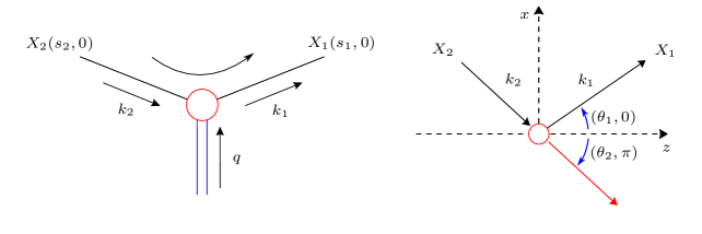
Figure 2: A diagram and a kinematic configuration of the scattering processes for two massless particles, $X_{1}$ and $X_{2}$, with the fermion line flowing from left to right. (Left) A spin-$s_{2}$ massless particle $X_{2}$ with the momentum $k_{2}$ is scattered with an external source, leading to the production of the spin-$s_{1}$ massless particle $X_{1}$ with the momentum $k_{1}$. (Right) The scattering processes are dealt with in a reference frame with a fixed coordinate system where $X_{1}$ and $X_{2}$ with the different energies are moving with the polar and azimuthal angles, $(\theta_{1},0)$ and $(\theta_{2},\pi)$, respectively. The red arrow is introduced for ease of comparison between the momenta $k_{1,2}$.

we can express the 1-to-1 matrix elements as

$$\langle k_{1},\lambda_{1}|\Theta^{[J;s_{1},s_{2}]}_{\mu}|k_{2},\lambda_{2}\rangle=\bar{\Theta}^{[J;s_{1},s_{2}]}_{(\lambda_{1},\lambda_{2})\mu}(k_{1},k_{2})$$

$$=\left\{\begin{array}[]{ll}\varepsilon^{*\alpha}(k_{1},\lambda_{1})\,\bar{\Gamma}^{[J;s_{1},s_{2}]}_{\alpha,\beta;\mu}(k_{1},k_{2})\,\varepsilon^{\beta}(k_{2},\lambda_{2})&\mbox{for bosonic cases}\\[3.0pt] \bar{u}^{\alpha}(k_{1},\lambda_{1})\,\bar{\Gamma}^{[J;s_{1},s_{2}]}_{\alpha,\beta;\mu}(k_{1},k_{2})\,u^{\beta}(k_{2},\lambda_{2})&\mbox{for fermionic cases}\end{array}\right.,$$ (171)

with the 1-to-1 covariant three-point vertices $\bar{\Gamma}(k_{1},k_{2})=\Gamma(k_{1},-k_{2})$ defined by the 0-to-2 vertices in Eq. (10) through the replacement $k_{2}\rightarrow-k_{2}$. Connecting the 1-to-1 and 0-to-2 matrix elements can be taken by means of the following crossing relations of the $X_{2}$ polarization vectors and Dirac spinors,

$$\varepsilon(k_{2},\pm)=-\varepsilon^{*}(k_{2},\mp)\quad\mbox{and}\quad u(k_{2},\pm\mbox{$\frac{1}{2}$})=-v(k_{2},\mp\mbox{$\frac{1}{2}$}),$$ (172)

which can be obtained straightforwardly by referring to their explicit structures in Eqs. (18) and (29).

Note that every bosonic basic operator involves a negative overall sign under the replacement $k_{2}\rightarrow-k_{2}$, but the fermionic operators are invariant due to the absence of momenta $k_{1,2}$. In addition, the replacement leads to the interchange of two combined momenta $p_{\mu}\leftrightarrow q_{\mu}$ and so the form-factor operators including them in Eq. (77) are replaced by

$$\big{[}\bar{\boldsymbol{F}}^{[J;s_{1},s_{2}]}_{(\lambda s_{1},\mp\lambda s_{2})}(k_{1},k_{2})\big{]}^{n}=\big{[}\boldsymbol{F}^{[J;s_{1},s_{2}]}_{(\lambda s_{1},\pm\lambda s_{2})}(k_{1},-k_{2})\big{]}^{n}$$

$$=\sum_{m=0}^{(J_{\mp}-n-\eta_{J_{\mp}-n})/2}\bar{A}^{[J;s_{1},s_{2}]}_{(\lambda s_{1},\mp\lambda s_{2});n,m}(k_{1},k_{2})\;\boldsymbol{p}^{n}\boldsymbol{q}^{J_{\mp}-n-2m}\boldsymbol{g}^{m},$$ (173)

in terms of the replaced form factors $\bar{A}_{(\lambda s_{1},\mp\lambda s_{2})}(k_{1},k_{2})\equiv A_{(\lambda s_{1},\pm\lambda s_{2})}(k_{1},-k_{2})$. Note that the $X_{2}$ helicity index gets a minus sign by the crossing relations in Eq. (172). For explicit calculations, we present the basic 1-to-1 matrix elements for the bosonic and fermionic basic operators:

$$\begin{array}[]{lll}\bar{S}^{\pm}_{\alpha,\beta}=-S^{\pm}_{\alpha,\beta}&\rightarrow&\bar{\Theta}^{[0;1,1]}_{(\lambda_{1},\lambda_{2})}(k_{1},k_{2})=+(k_{1}\cdot k_{2})\,\delta_{\lambda_{1},\pm}\delta_{\lambda_{1},-\lambda_{2}},\\[7.0pt] \bar{V}^{\pm}_{1\alpha;\mu}=-V^{\pm}_{1\alpha;\mu}&\rightarrow&\bar{\Theta}^{[1;1,0]}_{(\lambda_{1},0)\mu}(k_{1},k_{2})=+(k_{1}\cdot k_{2})\,\varepsilon^{*}_{1\bot\mu}(\pm)\,\delta_{\lambda_{1},\pm},\\[7.0pt] \bar{V}^{\pm}_{2\beta;\nu}=-V^{\mp}_{2\beta;\nu}&\rightarrow&\bar{\Theta}^{[1;0,1]}_{(0,\lambda_{2})\nu}(k_{1},k_{2})=-(k_{1}\cdot k_{2})\,\varepsilon_{2\bot\nu}(\pm)\,\delta_{\lambda_{2},\pm},\\[7.0pt] \bar{T}^{\pm}_{\alpha,\beta;\mu\nu}=-T^{\pm}_{\alpha,\beta;\mu\nu}&\rightarrow&\bar{\Theta}^{[2;1,1]}_{(\lambda_{1},\lambda_{2})\mu\nu}(k_{1},k_{2})=-(k_{1}\cdot k_{2})\big{[}\varepsilon^{*}_{1\bot\mu}(\pm)\varepsilon_{2\bot\nu}(\pm)+\mu\leftrightarrow\nu\,\big{]}\,\delta_{\lambda_{1},\pm}\delta_{\lambda_{1},\lambda_{2}},\end{array}$$ (178)

and,

$$\begin{array}[]{lll}\bar{\Sigma}^{\pm}=\Sigma^{\pm}&\rightarrow&\bar{\Theta}^{[0;\frac{1}{2},\frac{1}{2}]}_{(\lambda_{1},\lambda_{2})}(k_{1},k_{2})\,\;=i\sqrt{2k_{1}\cdot k_{2}}\;\delta_{\lambda_{1},\pm\frac{1}{2}}\,\delta_{\lambda_{1},-\lambda_{2}},\\[5.0pt] \bar{\Lambda}^{\pm}_{\mu}=\Lambda^{\pm}_{\mu}&\rightarrow&\bar{\Theta}^{[1;\frac{1}{2},\frac{1}{2}]}_{(\lambda_{1},\lambda_{2})\mu}(k_{1},k_{2})=-2i\sqrt{k_{1}\cdot k_{2}}\;\varepsilon^{*}_{1\bot\mu}(\pm)\,\delta_{\lambda_{1},\pm\frac{1}{2}}\,\delta_{\lambda_{1},\lambda_{2}},\end{array}$$ (181)

with the abbreviations $\varepsilon_{1,2\bot}(\pm)=\varepsilon_{\bot}(k_{1,2},\pm;k_{2,1})$. Collecting all the aspects of the crossing symmetry, we can observe that the diagonal and off-diagonal terms of 0-to-2 matrix elements correspond to the off-diagonal and diagonal terms of scattering matrix elements respectively,

$$\boldsymbol{\Theta}_{(\lambda_{1},\lambda_{2})}\leftrightarrow\bar{\boldsymbol{\Theta}}_{(\lambda_{1},-\lambda_{2})}.$$ (182)

It follows that the numbers of independent terms of the 0-to-2 covariant three-point vertices involving the selection rules of the decay process $\Psi\rightarrow XX$ in Tables. 1, 2, 3, and 4 can be employed fully in the analysis of the 1-to-1 matrix elements. Then, one can recognize straightforwardly that two massless particles of spins $s_{1,2}$ cannot carry the diagonal scattering matrix elements, i.e. $\bar{\boldsymbol{\Theta}}^{[J;s_{1},s_{2}]}_{(\pm s_{1},\pm s_{2})}=0$, for $J<s_{1}+s_{2}$ due to angular momentum conservation.

6.2 Discontinuity of the 1-to-1 matrix elements

In this section, we discuss how to identify explicitly the discontinuity between the 1-to-1 matrix elements for the spacelike $(k_{1}-k_{2})^{2}<0$ and lightlike $(k_{1}-k_{2})^{2}=0$ cases. Since every matrix element can be obtained by combining the basic matrix elements and form-factor operators, the task can be focused only on comparing the building blocks in the limiting $(k_{1}-k_{2})^{2}\rightarrow 0$ and lightlike $(k_{1}-k_{2})^{2}=0$ cases.

For the comparison, we first discuss the limiting case. As mentioned before, the covariant matrix elements take the same forms in every reference frame, thus, we choose a reference frame with a fixed coordinate system where their momenta $k_{1,2}$ on the $x$-$z$ plane are given by

$$k_{1}=k^{0}_{1}[1,\hat{n}(\theta_{1},0)]\quad\mbox{and}\quad k_{2}=k^{0}_{2}[1,\hat{n}(\theta_{2},\pi)],$$ (183)

with the unit vector $\hat{n}(\theta,\phi)$ in Eq. (16), satisfying $k_{1}\cdot k_{2}=k^{0}_{1}k^{0}_{2}[1-\cos(\theta_{1}+\theta_{2})]$ (see the kinematic configuration on the right panel in Fig. 2). The limits $\theta_{1,2}\rightarrow 0$ on the polar angles then lead to the two massless particles to move along the $z$ axis. In this frame, the polarization vectors of $X_{1,2}$ are given respectively by

$$\varepsilon(k_{1},\pm)=\frac{1}{\sqrt{2}}(0,\mp\cos\theta_{1},-i,\pm\sin\theta_{1})\quad\mbox{and}\quad\varepsilon(k_{2},\pm)=\frac{1}{\sqrt{2}}(0,\pm\cos\theta_{2},+i,\pm\sin\theta_{2}),$$ (184)

satisfying,

$$\begin{array}[]{l}\displaystyle\lim_{\theta_{1,2}\rightarrow 0}\sqrt{k_{1}\cdot k_{2}}\;\varepsilon^{*}_{\bot}(k_{1},\pm;k_{2})=\pm k,\\[10.0pt] \displaystyle\lim_{\theta_{1,2}\rightarrow 0}\sqrt{k_{1}\cdot k_{2}}\;\varepsilon_{\bot}(k_{2},\pm;k_{1})=\pm k,\end{array}$$ (187)

in terms of the covariant polarization vectors in Eq. (54) and the momentum $k=\sqrt{k_{1}^{0}k_{2}^{0}\,}(1,\hat{z})$ with the unit vector $\hat{z}=(0,0,1)$.

Employing Eqs. (178) and (181) with the covariant polarization vectors in Eq. (187), we obtain the following matrix elements for the basic operators in the limiting case,

$$\begin{array}[]{lll}\bar{S}^{\pm}_{\alpha,\beta}/(k_{1}\cdot k_{2})&\rightarrow&\displaystyle\lim_{\theta_{1,2}\rightarrow 0}\bar{\Theta}^{[0;1,1]}_{(\lambda_{1},\lambda_{2})}(k_{1},k_{2})=\delta_{\lambda_{1},\pm}\delta_{\lambda_{1},-\lambda_{2}},\\[7.0pt] \bar{V}^{\pm}_{1\alpha;\mu}/\sqrt{k_{1}\cdot k_{2}}&\rightarrow&\displaystyle\lim_{\theta_{1,2}\rightarrow 0}\bar{\Theta}^{[1;1,0]}_{(\lambda_{1},0)\mu}(k_{1},k_{2})=\pm k_{\mu}\,\delta_{\lambda_{1},\pm},\\[7.0pt] \bar{V}^{\pm}_{2\beta;\nu}/\sqrt{k_{1}\cdot k_{2}}&\rightarrow&\displaystyle\lim_{\theta_{1,2}\rightarrow 0}\bar{\Theta}^{[1;0,1]}_{(0,\lambda_{2})\nu}(k_{1},k_{2})=\mp k_{\nu}\,\delta_{\lambda_{2},\pm},\\[7.0pt] \bar{T}^{\pm}_{\alpha,\beta;\mu\nu}&\rightarrow&\displaystyle\lim_{\theta_{1,2}\rightarrow 0}\bar{\Theta}^{[2;1,1]}_{(\lambda_{1},\lambda_{2})\mu\nu}(k_{1},k_{2})=-2k_{\mu}k_{\nu}\,\delta_{\lambda_{1},\pm}\delta_{\lambda_{1},\lambda_{2}},\end{array}$$ (192)

and,

$$\begin{array}[]{lll}\bar{\Sigma}^{\pm}/\sqrt{k_{1}\cdot k_{2}}&\rightarrow&\displaystyle\lim_{\theta_{1,2}\rightarrow 0}\bar{\Theta}^{[0;\frac{1}{2},\frac{1}{2}]}_{(\lambda_{1},\lambda_{2})}(k_{1},k_{2})\,\;=i\sqrt{2}\;\delta_{\lambda_{1},\pm\frac{1}{2}}\,\delta_{\lambda_{1},-\lambda_{2}},\\[5.0pt] \bar{\Lambda}^{\pm}_{\mu}&\rightarrow&\displaystyle\lim_{\theta_{1,2}\rightarrow 0}\bar{\Theta}^{[1;\frac{1}{2},\frac{1}{2}]}_{(\lambda_{1},\lambda_{2})\mu}(k_{1},k_{2})=\mp 2ik_{\mu}\,\delta_{\lambda_{1},\pm\frac{1}{2}}\,\delta_{\lambda_{1},\lambda_{2}},\end{array}$$ (195)

with the appropriate normalizations of basic operators such that all of them yield nonzero matrix elements. the divergence-free property of the spin-1 polarization vector in Eq. (5) and the equality between the chirality and helicity for massless fermions enforce the basic operators in the lightlike case to be discontinuous to the limiting case:

$$\begin{array}[]{lll}\bar{S}^{\pm}_{\alpha,\beta}/(k_{1}\cdot k_{2})&\rightarrow&\bar{\Theta}^{[0;1,1]}_{(\lambda_{1},\lambda_{2})}(\overset{\circ}{k}_{1},\overset{\circ}{k}_{2})=\delta_{\lambda_{1},\lambda_{2}},\\[7.0pt] \bar{V}^{\pm}_{1\alpha;\mu}/\sqrt{k_{1}\cdot k_{2}}&\rightarrow&\bar{\Theta}^{[1;1,0]}_{(\lambda_{1},0)\mu}(\overset{\circ}{k}_{1},\overset{\circ}{k}_{2})=0,\\[7.0pt] \bar{V}^{\pm}_{2\beta;\nu}/\sqrt{k_{1}\cdot k_{2}}&\rightarrow&\bar{\Theta}^{[1;0,1]}_{(0,\lambda_{2})\nu}(\overset{\circ}{k}_{1},\overset{\circ}{k}_{2})=0,\\[7.0pt] \bar{T}^{\pm}_{\alpha,\beta;\mu\nu}&\rightarrow&\bar{\Theta}^{[2;1,1]}_{(\lambda_{1},\lambda_{2})\mu\nu}(\overset{\circ}{k}_{1},\overset{\circ}{k}_{2})=2k_{\mu}k_{\nu}\,\delta_{\lambda_{1},\lambda_{2}},\end{array}$$ (200)

and,

$$\begin{array}[]{lll}\bar{\Sigma}^{\pm}/\sqrt{k_{1}\cdot k_{2}}&\rightarrow&\displaystyle\lim_{\theta_{1,2}\rightarrow 0}\bar{\Theta}^{[0;\frac{1}{2},\frac{1}{2}]}_{(\lambda_{1},\lambda_{2})}(\overset{\circ}{k}_{1},\overset{\circ}{k}_{2})\,\;=0,\\[5.0pt] \bar{\Lambda}^{\pm}_{\mu}&\rightarrow&\displaystyle\lim_{\theta_{1,2}\rightarrow 0}\bar{\Theta}^{[1;\frac{1}{2},\frac{1}{2}]}_{(\lambda_{1},\lambda_{2})\mu}(\overset{\circ}{k}_{1},\overset{\circ}{k}_{2})=2k_{\mu}\,\delta_{\lambda_{1},\lambda_{2}},\end{array}$$ (203)

where the momenta $\overset{\circ}{k}_{1,2}=k^{0}_{1,2}(1,\hat{z})$ are introduced to deal with the lightlike cases generically. The differences in overall phases for the bosonic tensor and fermionic vector operators are caused by the $z$-axis rotation by the angle $\pi$ on the $X_{2}$ state in Eq. (183), implying their continuity.

Note that the continuity holds for all the terms in the form-factor operators including the term $q_{\mu}/\sqrt{k_{1}\cdot k_{2}}$ of which the invariance product is given by -1 regardless of the spacelike and lightlike cases. Thus, we can conclude as follows:

1. all the 1-to-1 matrix elements for the two massless particles with different spins must be discontinuous.

2. The continuity is violated even for the 1-to-1 matrix elements with the opposite-sign helicities of the identical-spin massless particles.

An interesting observation is that the basic bosonic scalar operators yield the nonzero basic matrix elements for the opposite (spacelike) and identical (lightlike) helicities of two massless particles. This is because the momentum-dependent terms are washed out due to the divergence-free property of the spin-1 polarization vector as mentioned before (see the explicit expressions of bosonic basic operators for the spacelike and lightlike cases in Appendix LABEL:sec:explicit_expressions_of_the_bosonic_operators).

6.3 1-to-1 matrix elements of conserved tensor currents

Theoretically, a conserved tensor current $\Theta^{[J;s,s]}_{\mu_{1}\cdots\mu_{J}}$ of a spin-$s$ massless particle is defined to satisfy the following relations,

$$\partial^{\mu_{i}}\Theta_{\mu_{1}\cdots\mu_{i}\cdots\mu_{J}}(x) =0,$$ (204)

$$\int d^{3}\vec{x}\;\Theta_{0\,\mu_{2}\cdots\mu_{i}\cdots\mu_{J}}(x)|k,\lambda\rangle =Q\,k_{\mu_{2}}\cdots k_{\mu_{J}}|k,\lambda\rangle,$$ (205)

in terms of the conserved quantity $Qk_{\mu_{2}}\cdots k_{\mu_{J}}$ with a real constant $Q$. However, one is able to not require the second condition implying the continuity of the 1-to-1 matrix elements if it is assumed that a conserved quantity is determined by measuring the nearly forward scattering caused by the exchange of a spacelike but nearly lightlike massless particle as stated in the paper of Weinberg and Witten [12]. Furthermore, the validity of the assumption is checked concretely by employing the physical particle state with no definite momentum in Ref. [17].

As implied in Sec. 4, one can construct the covariant three-point vertices even yielding the noncovariant matrix elements in the covariant formulation. Referring to the discontinuity of matrix elements discussed in Sec. 6.2 one can construct all covariant three-point vertices for conserved tensor currents. To do so, we define several alternative basic operators as

$$\begin{array}[]{lll}S_{c\,\alpha,\beta}=-g_{\alpha\beta}&\rightarrow&\bar{\Theta}^{[0;1,1]}_{(\lambda_{1},\lambda_{2})}(\overset{\circ}{k}_{1},\overset{\circ}{k}_{2})=\delta_{\lambda_{1},\lambda_{2}},\\ T_{c\,\alpha,\beta;\mu\nu}=[\wick{k_{1}\c{1}\rho\alpha\mu]_{+}[k_{2}\c{1}\sigma\beta\nu}]_{+}-[\wick{k_{1}\c{1}\rho\alpha\mu]_{-}[k_{2}\c{1}\sigma\beta\nu}]_{-}&\rightarrow&\bar{\Theta}^{[2;1,1]}_{(\lambda_{1},\lambda_{2})}(\overset{\circ}{k}_{1},\overset{\circ}{k}_{2})=2k_{\mu}k_{\nu}\,\delta_{\lambda_{1},\lambda_{2}},\end{array}$$ (208)

and,

$$\begin{array}[]{lll}\Lambda_{c\,\mu}=\gamma_{\mu}&\rightarrow&\bar{\Theta}^{[1;\frac{1}{2},\frac{1}{2}]}_{(\lambda_{1},\lambda_{2})}(\overset{\circ}{k}_{1},\overset{\circ}{k}_{2})=2k_{\mu}\,\delta_{\lambda_{1},\lambda_{2}},\end{array}$$ (210)

yielding nonzero basic matrix elements only for the identical-sign helicities in the lightlike case. Note that the scalar operator $S_{c}$ does not involve the covariant matrix elements. By collecting the alternative basic and momentum $p_{\mu}$ operators appropriately, we can obtain the covariant three-point vertices of conserved tensor currents as

$$\boldsymbol{\Gamma}^{[J;s,s]}_{\scriptsize\mbox{c}}=Q\,\boldsymbol{p}^{J-2n}\,\boldsymbol{T}^{n}_{c}\,\boldsymbol{S}^{s-n}_{c},$$ (211)

for bosonic cases, and

$$\boldsymbol{\Gamma}^{[J;s,s]}_{\scriptsize\mbox{c}}=Q\,\boldsymbol{p}^{J-2n-1}\,\boldsymbol{\Lambda}_{c}\,\boldsymbol{T}^{n}_{c}\,\boldsymbol{S}^{s-n-1/2}_{c},$$ (212)

for fermionic cases with a real constant $Q$ in a compact operator form where the nonnegative integer $n$ can be chosen arbitrarily under the conditions $J\leq 2n$ and $s\leq n$.

In order to hold the covariance of conserved tensor currents, it is required to set $n=s$ and $n=s-1/2$ for bosonic and fermionic cases respectively due to the appearance of the operator $S_{c}$ involving the noncovariant basic matrix elements. It enables us to find the limits on the conserved current $J_{\mu}$ and energy-momentum tensor $T_{\mu\nu}$ of a massless particle:

1. The covariance of $J_{\mu}$ and $T_{\mu\nu}$ of a spin-$s$ massless particle holds only for $s\leq 1/2$ and $s\leq 1$ respectively.

2. Oppositely, no noncovariant $J_{\mu}$ and $T_{\mu\nu}$ can exist for $s\leq 1/2$ and $s\leq 1$ respectively.

3. The structures of the noncovariant $J_{\mu}$ and $T_{\mu\nu}$ for $s>1/2$ and $s>1$ respectively are not uniquely determined.

The first finding is exactly equal to the theorem developed by Weinberg and Witten. The second one indicates that it is forbidden to construct a theory including spin-$s$ massless particles of which charges or energies and momenta are not measurable in experiments when $s\leq 1/2$ and $s\leq 1$ respectively, i.e. the charges or energies and momenta of such massless particles must have local weights. Contrarily, the third one indicates that the spin-$s$ massless particles satisfying $s\leq 1/2$ and $s\leq 1$ can be included in a theory only when their charges or energies and momenta respectively are not measurable in experiments, such as the gluon and graviton involving the noncovariant conserved current and energy-momentum tensor [17].

7 Conclusion

We have presented an efficient algorithm to construct all the matrix elements of covariant tensor currents of massless particles of any spins in the covariant formulation. The matrix elements are expressed in a helicity basis adopting the Wick convention. The construction has been taken first in the two-body decay of an integer spin-$J$ particle $\Psi^{(*)}$ into two massless particles of arbitrary spins $s_{1,2}$. To cover the off-shell $\Psi^{*}$ decay, we have taken only the least constraint on the covariant tensor currents which is the symmetricity of the tensor currents.

After deriving all the basic and form-factor operators which are the basic building blocks involving basic matrix elements, we have constructed the general three-point vertices of an off-shell particle and two massless particles straightforwardly by assembling the building blocks according to our algorithm. All the matrix elements can be extracted directly from the covariant three-point vertices as the wave tensors of massless particles are determined regardless of their interactions. In the construction of basic operators, we have found more fundamental structures of basic bosonic tensor operators than those given in the prototype [19] of our algorithm. The revised basic operators would be more useful in extending the algorithm to cover more general event topologies.

Employing the constructed three-point vertices, we have shown the selection rules for the decay of an off-shell massive particle into two identical massless particles of any spin, which are the generalization of the Landau-Yang theorem. The 1-to-1 matrix elements were derived from the 0-to-2 matrix elements by utilizing the crossing symmetry. Taking the lightlike limit on the matrix elements with the spacelike momentum transfer, we have investigated the discontinuity of all the basic matrix elements, resulting in the full identification of the discontinuity of all the matrix elements. Finally, we have constructed the covariant three-point vertices for all the conserved tensor currents with the introduction of several alternative basic operators. From the vertices, we have extracted the WW theorem directly with additional limits on massless particles including high spins.

As a natural extension of this work, the development of an algorithm for constructing all the covariant three-point vertices for all the off-shell particles is under study at present. In addition, the construction of all the four-point vertices will be reported separately. After finishing the extensions, a program to generate all the three- and four-point vertices and the corresponding Lagrangian operators will be presented for ease of usage of the algorithm. All of these extensions will enable us to deal with straightforwardly the phenomenological and theoretical aspects of exotic interactions of particles including high spins.

Appendix A Explicit expressions of the bosonic basic operators

In this section, we present the explicit expressions of all the bosonic basic operators for the spacelike and lightlike momentum transfers.

A.1 Spacelike case $(k_{1}-k_{2})^{2}<0$

Employing the polarization-covariant operators in Eqs. (35) to (38), we can calculate the basic scalar and vector operators as

$$S^{\pm}_{\alpha\beta} \;\overset{\scriptsize\mbox{eff}}{=}\;\frac{1}{2}\Big{[}-(k_{1}\cdot k_{2})g_{\alpha\beta}+k_{2\alpha}k_{1\beta}\pm ik_{1}^{\rho}k_{2}^{\sigma}\varepsilon_{\rho\sigma\alpha\beta}\Big{]},$$ (213)

$$V^{\pm}_{1\alpha\mu} \;\overset{\scriptsize\mbox{eff}}{=}\;\frac{1}{2}\Big{[}-(k_{1}\cdot k_{2})g_{\alpha\mu}+k_{2\alpha}k_{1\mu}\pm ik_{1}^{\rho}k_{2}^{\sigma}\varepsilon_{\rho\sigma\alpha\mu}\Big{]},$$ (214)

$$V^{\pm}_{2\beta\mu} \;\overset{\scriptsize\mbox{eff}}{=}\;\frac{1}{2}\Big{[}-(k_{1}\cdot k_{2})g_{\beta\nu}+k_{1\beta}k_{2\mu}\pm ik_{2}^{\sigma}k_{1}^{\rho}\varepsilon_{\sigma\rho\beta\mu}\Big{]},$$ (215)

with the absence of the terms involving $k_{1\alpha}$ or $k_{2\beta}$ due to the divergence-free property of polarization vectors. Employing the effective identities in Eqs. (60) and (65), the bosonic tensor operators can be written effectively as

$$T^{\pm}_{\alpha\beta;\mu\nu} \overset{\scriptsize\mbox{eff}}{=}\;\frac{1}{2}\bigg{\{}\Big{[}-(k_{1}\cdot k_{2})g_{\alpha\mu}g_{\beta\nu}+g_{\alpha\mu}k_{1\beta}k_{2\nu}+g_{\beta\nu}k_{2\alpha}k_{1\mu}-k_{1\mu}k_{2\nu}g_{\alpha\beta}-\mu\leftrightarrow\nu\Big{]}$$

$$-g_{\mu\nu}\Big{[}(k_{1}\cdot k_{2})g_{\alpha\beta}-k_{2\alpha}k_{1\beta}\Big{]}\pm i\Big{[}g_{\alpha\mu}k^{\sigma}_{2}k^{\rho}_{1}\varepsilon_{\sigma\rho\beta\nu}-k_{1\mu}k^{\sigma}_{2}\varepsilon_{\sigma\alpha\beta\nu}+\mu\leftrightarrow\nu\Big{]}\pm ig_{\mu\nu}k_{1}^{\rho}k_{2}^{\sigma}\varepsilon_{\rho\sigma\alpha\beta}\bigg{\}},$$ (216)

with the exchange $\mu\leftrightarrow\nu$ between two four-vector indices, $\mu$ and $\nu$.

A.2 Lightlike case $(k_{1}-k_{2})^{2}=0$

In the lightlike case with the momenta $\overset{\circ}{k}_{1,2}=k^{0}_{1,2}(1,\hat{z})$, all the odd-parity contractions vanish due to the antisymmetric property of the Levi-Civita tensor. In addition, the divergence-free property of polarization vectors removes all the momenta involving the four-factor indices, $\alpha$ and $\beta$, in the basic operators. Thus, the basic operators can be effectively given by

$$S^{\pm}_{\alpha\beta}/(\overset{\circ}{k}_{1}\cdot\overset{\circ}{k}_{2})\overset{\scriptsize\mbox{eff}}{=}-g_{\alpha\beta},\quad\;\;V^{\pm}_{1\alpha\mu}/(\overset{\circ}{k}_{1}\cdot\overset{\circ}{k}_{2})\overset{\scriptsize\mbox{eff}}{=}-g_{\alpha\mu},\quad\;\;V^{\pm}_{2\beta\mu}/(\overset{\circ}{k}_{1}\cdot\overset{\circ}{k}_{2})\overset{\scriptsize\mbox{eff}}{=}-g_{\beta\mu},$$ (217)

and,

$$T^{\pm}_{\alpha\beta;\mu\nu}\overset{\scriptsize\mbox{eff}}{=}-k_{\mu}k_{\nu}g_{\alpha\beta}.$$ (218)

with the momentum $k=\sqrt{k_{1}^{0}k_{2}^{0}}(1,\hat{z})$ and the invariant product $(\overset{\circ}{k}_{1}\cdot\overset{\circ}{k}_{2})$ introduced for comparing the limiting case $(k_{1}-k_{2})^{2}\rightarrow 0$ and the lightlike case $(k_{1}-k_{2})^{2}=0$ in Sec. 6.2. .

References

- [1] S. L. Glashow, Nucl. Phys. 22, 579-588 (1961) doi:10.1016/0029-5582(61)90469-2; S. Weinberg, Phys. Rev. Lett. 19, 1264-1266 (1967) doi:10.1103/PhysRevLett.19.1264; A. Salam, Conf. Proc. C 680519, 367-377 (1968) doi:10.1142/9789812795915_0034; H. Fritzsch, M. Gell-Mann and H. Leutwyler, Phys. Lett. B 47, 365-368 (1973) doi:10.1016/0370-2693(73)90625-4;
- [2] G. Aad et al. [ATLAS], Phys. Lett. B 716 (2012), 1-29 doi:10.1016/j.physletb.2012.08.020 [arXiv:1207.7214 [hep-ex]]. S. Chatrchyan et al. [CMS], Phys. Lett. B 716 (2012), 30-61 doi:10.1016/j.physletb.2012.08.021 [arXiv:1207.7235 [hep-ex]].
- [3] G. Bertone, D. Hooper and J. Silk, Phys. Rept. 405, 279-390 (2005) doi:10.1016/j.physrep.2004.08.031 [arXiv:hep-ph/0404175 [hep-ph]].
- [4] Y. Fukuda et al. [Super-Kamiokande], Phys. Rev. Lett. 81, 1562-1567 (1998) doi:10.1103/PhysRevLett.81.1562 [arXiv:hep-ex/9807003 [hep-ex]]. R. N. Mohapatra and G. Senjanovic, Phys. Rev. Lett. 44, 912 (1980) doi:10.1103/PhysRevLett.44.912;
- [5] M. Dine and A. Kusenko, Rev. Mod. Phys. 76, 1 (2003) doi:10.1103/RevModPhys.76.1 [arXiv:hep-ph/0303065 [hep-ph]]; T. Asaka and M. Shaposhnikov, Phys. Lett. B 620, 17-26 (2005) doi:10.1016/j.physletb.2005.06.020 [arXiv:hep-ph/0505013 [hep-ph]].
- [6] P. A. Zyla et al. [Particle Data Group], PTEP 2020, no.8, 083C01 (2020) doi:10.1093/ptep/ptaa104.
- [7] M. Fierz and W. Pauli, Proc. Roy. Soc. Lond. A 173, 211-232 (1939) doi:10.1098/rspa.1939.0140 J. Fang and C. Fronsdal, Phys. Rev. D 18, 3630 (1978) doi:10.1103/PhysRevD.18.3630; C. Fronsdal, Phys. Rev. D 18, 3624 (1978) doi:10.1103/PhysRevD.18.3624; F. A. Berends, J. W. van Holten, B. de Wit and P. van Nieuwenhuizen, J. Phys. A 13, 1643-1649 (1980) doi:10.1088/0305-4470/13/5/022;
- [8] S. Weinberg, Phys. Rev. 134, B882-B896 (1964) doi:10.1103/PhysRev.134.B882;
- [9] B. de Wit and D. Z. Freedman, Phys. Rev. D 21, 358 (1980) doi:10.1103/PhysRevD.21.358; A. K. H. Bengtsson, I. Bengtsson and L. Brink, Nucl. Phys. B 227, 31-40 (1983) doi:10.1016/0550-3213(83)90140-2; A. K. H. Bengtsson, I. Bengtsson and N. Linden, Class. Quant. Grav. 4, 1333 (1987) doi:10.1088/0264-9381/4/5/028;
- [10] T. Curtright, Phys. Lett. B 85, 219-224 (1979) doi:10.1016/0370-2693(79)90583-5; C. Aragone and S. Deser, Nucl. Phys. B 170, 329-352 (1980) doi:10.1016/0550-3213(80)90153-4; M. A. Vasiliev, Yad. Fiz. 32, 855-861 (1980); M. S. Plyushchay, Mod. Phys. Lett. A 4, 2747-2755 (1989) doi:10.1142/S0217732389003075;
- [11] L. D. Landau, Dokl. Akad. Nauk SSSR 60 (1948) no.2, 207-209 doi:10.1016/B978-0-08-010586-4.50070-5; C. N. Yang, Phys. Rev. 77 (1950), 242-245 doi:10.1103/PhysRev.77.242;
- [12] S. Weinberg and E. Witten, Phys. Lett. B 96 (1980), 59-62 doi:10.1016/0370-2693(80)90212-9
- [13] M. Porrati, Phys. Rev. D 78 (2008), 065016 doi:10.1103/PhysRevD.78.065016 [arXiv:0804.4672 [hep-th]].
- [14] S. Weinberg, Phys. Rev. 135, B1049-B1056 (1964) doi:10.1103/PhysRev.135.B1049; F. A. Berends, G. J. H. Burgers and H. van Dam, Nucl. Phys. B 260, 295-322 (1985) doi:10.1016/0550-3213(85)90074-4; X. Bekaert, N. Boulanger and S. Leclercq, J. Phys. A 43, 185401 (2010) doi:10.1088/1751-8113/43/18/185401 [arXiv:1002.0289 [hep-th]]. A. K. H. Bengtsson and I. Bengtsson, Class. Quant. Grav. 3, 927-936 (1986) doi:10.1088/0264-9381/3/5/022;
- [15] S. Y. Choi and J. H. Jeong, Phys. Rev. D 103 (2021) no.9, 096013 doi:10.1103/PhysRevD.103.096013 [arXiv:2102.11440 [hep-ph]].
- [16] V. Pleitez, [arXiv:1508.01394 [hep-ph]]. X. Bekaert, N. Boulanger and P. Sundell, Rev. Mod. Phys. 84 (2012), 987-1009 doi:10.1103/RevModPhys.84.987 [arXiv:1007.0435 [hep-th]]. R. Rahman, PoS ModaveVIII, 004 (2012) doi:10.22323/1.195.0004 [arXiv:1307.3199 [hep-th]].
- [17] F. Loebbert, Annalen Phys. 17, 803-829 (2008) doi:10.1002/andp.200810305
- [18] B. P. Abbott et al. [LIGO Scientific and Virgo], Phys. Rev. Lett. 116, no.6, 061102 (2016) doi:10.1103/PhysRevLett.116.061102 [arXiv:1602.03837 [gr-qc]].
- [19] S. Y. Choi and J. H. Jeong, Phys. Rev. D 104 (2021) no.5, 055046 doi:10.1103/PhysRevD.104.055046 [arXiv:2106.15774 [hep-ph]]; S. Y. Choi and J. H. Jeong, Phys. Rev. D 105 (2022) no.1, 016016 doi:10.1103/PhysRevD.105.016016 [arXiv:2111.08236 [hep-ph]].
- [20] M. Jacob and G. C. Wick, Annals Phys. 7, 404-428 (1959) doi:10.1016/0003-4916(59)90051-X.
- [21] G. C. Wick, Annals Phys. 18, 65-80 (1962) doi:10.1016/0003-4916(62)90059-3
- [22] S. U. Chung, doi:10.5170/CERN-1971-008; E. Leader, Camb. Monogr. Part. Phys. Nucl. Phys. Cosmol. 15, pp.1-500 (2011) 2011, ISBN 978-0-511-87418-5, 978-0-521-35281-9, 978-0-521-02077-0
- [23] S. U. Chung, Phys. Rev. D 57 (1998), 431-442 doi:10.1103/PhysRevD.57.431; S. Cotogno, C. Lorcé, P. Lowdon and M. Morales, Phys. Rev. D 101, no.5, 056016 (2020) doi:10.1103/PhysRevD.101.056016 [arXiv:1912.08749 [hep-ph]]. C. Lorcé and P. Lowdon, Phys. Rev. D 102, 125013 (2020) doi:10.1103/PhysRevD.102.125013 [arXiv:2004.13057 [hep-th]].
- [24] E. C. G. Sudarshan, Phys. Rev. D 24, 1591-1594 (1981) doi:10.1103/PhysRevD.24.1591
- [25] S. Z. Huang, P. F. Zhang, T. N. Ruan, Y. C. Zhu and Z. P. Zheng, Eur. Phys. J. C 42 (2005), 375-389 doi:10.1140/epjc/s2005-02299-4
- [26] K. Hayashi, Prog. Theor. Phys. 41, 214-232 (1969) doi:10.1143/PTP.41.214, F. T. Brandt, J. Frenkel and D. G. C. McKeon, Phys. Rev. D 76, 105029 (2007) doi:10.1103/PhysRevD.76.105029 [arXiv:0707.2590 [hep-th]], F. T. Brandt, D. G. C. McKeon and C. Zhao, Phys. Rev. D 96, no.12, 125009 (2017) doi:10.1103/PhysRevD.96.125009 [arXiv:1705.07891 [hep-th]].
- [27] R. E. Behrends and C. Fronsdal, Phys. Rev. 106, no.2, 345 (1957) doi:10.1103/PhysRev.106.345; P. R. Auvil and J. J. Brehm, Phys. Rev. 145, no.4, 1152 (1966) doi:10.1103/PhysRev.145.1152; P. J. Caudrey, I. J. Ketley and R. C. King, Nucl. Phys. B 6, 671-686 (1968) doi:10.1016/0550-3213(68)90181-8; M. D. Scadron, Phys. Rev. 165, 1640-1647 (1968) doi:10.1103/PhysRev.165.1640; S. Z. Huang, T. N. Ruan, N. Wu and Z. P. Zheng, Eur. Phys. J. C 26, 609-623 (2003) doi:10.1140/epjc/s2002-01026-1.
- [28] S. Weinberg, Phys. Rev. 133, B1318-B1332 (1964) doi:10.1103/PhysRev.133.B1318
- [29] F. Boudjema and C. Hamzaoui, Phys. Rev. D 43, 3748-3758 (1991) doi:10.1103/PhysRevD.43.3748