Discovery of two promising isolated neutron star candidates in the SRG/eROSITA All-Sky Survey

We report the discovery of the isolated neutron star (INS) candidates eRASSU~J065715.3+260428 and eRASSU~J131716.9-402647 from the Spectrum Roentgen Gamma (SRG) eROSITA All-Sky Survey. Selected for their soft X-ray emission and absence of catalogued counterparts, both objects were recently targeted with the Large Binocular Telescope and the Southern African Large Telescope. The absence of counterparts down to deep optical limits (25 mag, 5$\sigma$) and, as a result, large X-ray-to-optical flux ratios in both cases strongly suggest an INS nature. The X-ray spectra of both sources are well described by a simple absorbed blackbody, whereas other thermal and non-thermal models (e.g. a hot-plasma emission spectrum or power law) are disfavoured by the spectral analysis. Within the current observational limits, and as expected for cooling INSs, no significant variation ($>2\sigma$) has been identified over the first two-year time span of the survey. Upcoming dedicated follow-up observations will help us to confirm the candidates’ nature.

1 Introduction

The majority of the known Galactic isolated neutron star (INS) population consists of radio and $\gamma$-ray pulsars and recycled millisecond pulsars. Powered by the loss of rotational energy (Becker, 2009), these objects are preferentially detected in large-scale radio surveys. More elusive are ’magnetars’ (see, e.g. Kaspi & Beloborodov, 2017, for a review), which are driven by their super strong magnetic energy; the young and atypical central compact objects (CCOs) in supernova remnants (De Luca, 2017); and the radio-quiet, so-called X-ray dim isolated neutron stars (XDINSs, Turolla, 2009). In particular, XDINSs are well known for their purely thermal spectra, with no significant traces of magnetospheric or accretion activity. Only recently were weak non-thermal emission components detected in the cumulative X-ray spectra of the XDINS RX~J1856.5-3754 and RX~J0420.0-5022 (Dessert et al., 2020; De Grandis et al., 2022). XDINSs possess spin periods ranging from 3–17 s, which, under the assumption of magneto-dipole radiation being solely responsible for the observed braking of the neutron star rotation (Ostriker & Gunn, 1969), imply spin-down ages on the million year timescale. Nevertheless, XDINSs are powered by thermal emission and not magnetic braking, and thus kinematic age estimates of the order of $0.5-1$ Myr (Tetzlaff et al., 2010, 2011, 2012) are deemed more reliable, whereas statistical age estimates suffer from the small known population (Gill & Heyl, 2013). In comparison to similarly aged rotation-powered pulsars, XDINSs possess larger spin periods, stronger magnetic field strengths ($10^{13}-10^{14}$ G), and higher thermal luminosities.

Originally discovered in ROSAT observations (see Haberl, 2007, for details), the seven known XDINSs are rather nearby and could be as common as rotation-powered pulsars. Keane & Kramer (2008) estimated that the total INS birthrate exceeds the Galactic core-collapse supernova rate, which might imply evolutionary connections between the different classes of INSs. This is supported by state-of-the art magnetothermal evolutionary models that suggest XDINSs are evolved magnetars (Viganò et al., 2013). The small number of confirmed XDINSs makes it difficult to investigate population properties on the Galactic scale and to confirm evolutionary links with other INS families. Thus, attempts have been made since their initial discovery to find new members. Most notable are the identification of Calvera (Rutledge et al., 2008), a fast-spinning INS whose exact nature is still under debate (Bogdanov et al., 2019); 2XMM~J104608.7-594306, a seemingly cooling neutron star in the Carina Nebula (Pires et al., 2009, 2015); and the four INS candidates recently selected from the XMM-Newton footprint (Rigoselli et al., 2022). Among these, 4XMM J022141.5-735632 appears particularly promising on the basis of its purely thermal X-ray emission and stable properties (Pires et al., 2022).

Table 1: Properties of the two targets from eRASS:4.

Target	RA	Dec	Error	$N_{\rm H}^{\rm Gal}$	$b$	Flux	HR1	HR2	HR3
eRASSU	[°]	[°]	[″]	[$10^{20}$ cm-2]	[°]
J065715.3+260428	$104.3140$	$26.0746$	$1.3$	$8.3$	12.75	$2.21(26)$	$0.33(11)$	$-0.79(9)$	$-1.00(26)$
J131716.9-402647	$199.3204$	$-40.4462$	$0.9$	$6.7$	22.16	$4.52(28)$	$0.42(6)$	$-0.83(4)$	$-0.92(18)$

The discovery of additional XDINS candidates beyond the solar vicinity has been met with difficulties in the past. While the ROSAT survey (Voges et al., 1999) covers the full sky, the large positional errors at faint X-ray fluxes make the selection of new candidates impractical due to source confusion. X-ray catalogues based on instruments that offer a better localisation and often reach fainter fluxes (e.g. XMM-Newton or Chandra) are limited by the small sky coverage. The eROSITA All-Sky Survey (eRASS, Predehl et al., 2021) is conducting the deepest imaging of the entire X-ray sky since the days of ROSAT. At soft X-ray energies, eRASS ought to surpass its predecessor by a factor of 20 in sensitivity (Merloni et al., 2012), with a much improved spectral resolution and positional accuracy. Flux-limited searches over the German part of the eROSITA sky thence offer the unique opportunity to unveil their numbers and birthrate beyond the immediate solar vicinity (Pires et al., 2017). To this end, we searched the eRASS catalogues for X-ray sources with properties consistent with those of INSs. We followed the brightest among our candidates up with the Large Binocular Telescope (LBT, Hill et al., 2012) and Southern African Large Telescope (SALT, Buckley et al., 2006) to rule out other soft X-ray emitters that are known to contaminate our sample. We present in this work the first two promising INS candidates resulting from our ongoing identification campaign, eRASSU~J065715.3+260428 and eRASSU~J131716.9-402647 (hereafter dubbed J0657 and J1317).

The paper is structured as follows. In Sect. 2 we present the applied search strategy and the available observations at optical and X-ray energies. We present the properties inferred from the X-ray spectra and the obtained optical magnitude limits in Sect. 3 and we discuss the results in Sect. 4.

2 Observations and data reduction

Table 2: X-ray and optical observations of J0657 and J1317.

Target	Telescope	Date of	Cts	Texp
		Observation		[s]
J0657	eROSITA	2020-04-11	21	$126$
J0657	eROSITA	2020-10-14/15	19	$130$
J0657	eROSITA	2021-04-10/11	30	$157$
J0657	eROSITA	2021-10-12/13	26	$185$
J1317	eROSITA	2020-01-19/20/21	107	$353$
J1317	eROSITA	2020-07-21/22/23	104	$345$
J1317	eROSITA	2021-01-15/16	75	$222$
J1317	eROSITA	2021-07-23/24	70	$230$
J1317	eROSITA	2022-01-21/22	62	$247$
J0657	LBT	2021-12-05		$400$
J0657	LBT	2022-04-01		$400$
J1317	SALT	2022-05-26		$2400$

2.1 Target selection

Since the start of the survey observations in December 2019, eROSITA has completed four out of the eight planned full sky scans and started the fifth. We searched the single scan and stacked (which combines all four completed surveys, dubbed eRASS:4) catalogues for possible candidates above flux values of $10^{-13}$erg s^-1 cm^-2 (0.2–2.0 keV). The eRASS will contain fainter INSs, but those objects are difficult to separate from other soft X-ray emitting sources based on the currently available positional accuracy alone. At the same time, the necessary optical follow-up observations will be expensive (see Pires et al. (2017); Khokhryakova et al. (2021) for the prospect of INS searches in eRASS), so the confirmation of fainter candidates is best left to the next generation of large telescopes (e.g. ESO-ELT) and/or sky surveys (e.g. the LSST, Ivezić et al., 2019).

The known XDINSs are characterised by their soft X-ray spectra, which are well described by absorbed blackbody emission, with effective temperatures between 40–100 eV (Haberl, 2007). Using counts in neighbouring energy bands to compute hardness ratios, the soft nature can be translated into hardness ratio constraints. The applied cuts (using hardness ratios computed between the 0.2–0.5 keV and 0.5–1 keV, the 0.5–1 keV and 1–2 keV, and the 1–2 keV and 2–5 keV bands) were defined based on XSPEC (Arnaud, 1996, version: 12.12.0) simulations of absorbed blackbody spectra with $N_{\rm H}$ values ranging from $0-10^{23}$ cm^-2 and effective temperatures between 30–250 eV. The resulting cuts are shown in Fig. 1.

XDINSs possess X-ray-to-optical flux ratio values of $\log(f_{\mathrm{X}}/f_{\mathrm{opt,V}})\geq 4.0$ (Kaplan et al., 2003). Thus, at the X-ray flux level chosen, optical counterparts are expected to be fainter than magnitude 29, which is too faint to be detected in publicly available wide-area surveys and databases (e.g. the 5$\sigma$ r-band detection limits of the deepest used optical surveys in this work, namely Pan-STARRS DR1 (Chambers et al., 2016) and Legacy Survey DR9/10 (Dey et al., 2019), are located at 23.2 mag and 24–25.3 mag, respectively). This allows one to select candidates by requiring for the absence of optical/infrared (IR) counterparts. Specifically, we conducted a probabilistic cross-matching of the eRASS position against the GAIA DR3 (Gaia Collaboration et al., 2022b), Pan-STARRS DR1, and Legacy Survey DR9/10 catalogues using the ARCHES X-Match tool (Pineau et al., 2017). We kept candidates with non-matching probabilities in excess of 50%. Additionally, we excluded sources with counterparts in the SIMBAD database (Wenger et al., 2000), the VISTA Hemisphere Survey (McMahon et al., 2013), and the CatWISE2020 (Marocco et al., 2021) catalogues.

To exclude other potential identifications – for example X-ray emitting stars, active galactic nuclei (AGN), or cataclysmic variables –, additional observations at optical energies are necessary. Thus, we initiated a follow-up campaign with LBT and SALT, to confirm the absence of counterparts at fainter magnitudes. While this observational campaign is still ongoing, optical imaging has already been conducted for J0657 and J1317 (Table 2). A paper reporting on the full search results in the eRASS catalogues will be presented in another work (Kurpas et al., in preparation).

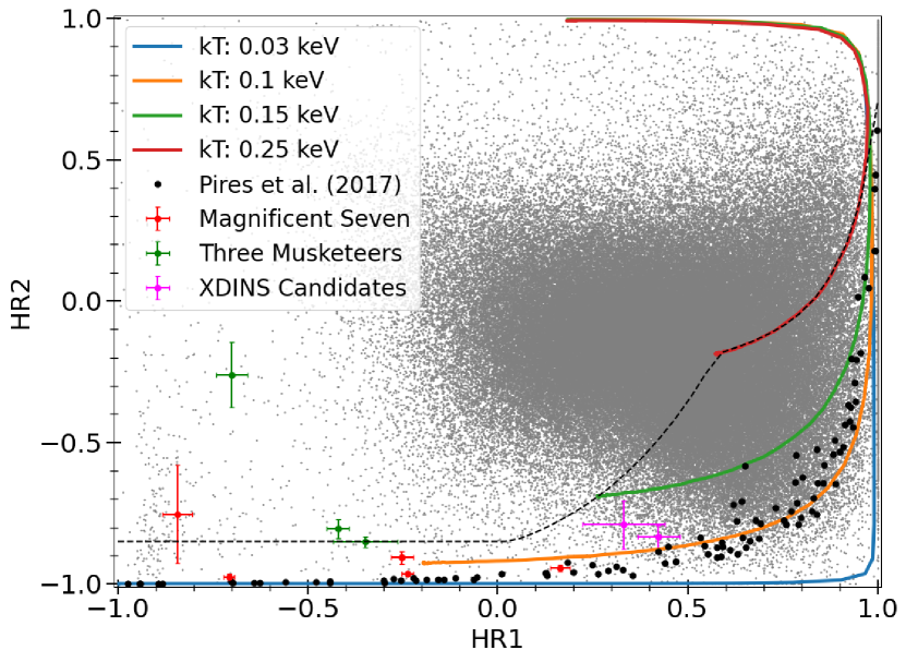
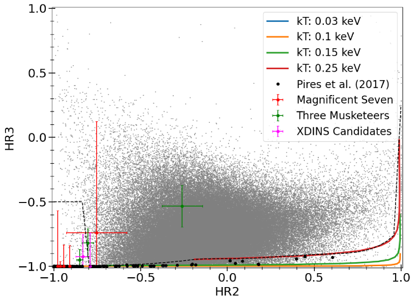
Figure 1: Hardness ratio diagrams indicating the applied selection (dashed black line), the distribution of simulated absorbed blackbody spectra (solid lines), and the position of the synthetic thermally emitting INS population of Pires et al. (2017) (black circles). The known population of XDINSs (dubbed the ‘magnificent seven’), on the German part of the eROSITA sky, in red, and the three middle-aged thermally emitting rotation-powered pulsars, PSR~B0656+14, Geminga, and PSR~B1055-52 (dubbed the ‘three musketeers’) in green are indicated along with the location of the two INS candidates discussed in this work (magenta). The hardness ratios were computed between the 0.2–0.5 keV and 0.5–1.0 keV (HR1), 0.5–1.0 keV and 1.0–2.0 keV (HR2), and 1.0–2.0 keV and 2.0–5.0 keV (HR3) bands.

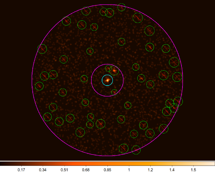
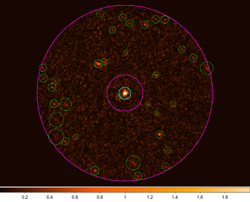
Figure 2: Stacked eRASS source (cyan circle, 1′ radius) and background (magenta annulus, 3′ inner and 15′ outer radius) regions for J0657 (left) and J1317 (right). Field sources discovered from a source detection run, using all telescopes (TM0) and photons in the 0.2–10 keV band, were excluded from the source and background region (green circles). The images include photons from the same telescope and energy band configuration that was used for the source detection.

Table 3: X-ray spectral fitting results for both candidates.

BB
Source	$N_{\rm H}$	$kT$	Radius	log(Z)	log(ZBB/Z)	AIC	Absorbed flux
	[$10^{20}$ cm-2]	[eV]	[km]				[$10^{-13}$ erg s-1 cm-2]
J0657	$5^{+5}_{-4}$	$108^{+15}_{-14}$	$1.9^{+1.4}_{-0.7}$	-37.4	0	65.7	$2.29^{+0.29}_{-0.26}$
J1317	$10.2^{+3}_{-2.8}$	$110^{+7}_{-7}$	$3.0^{+0.9}_{-0.7}$	-71.2	0	128.5	$4.40^{+0.25}_{-0.24}$
apec
Source	$N_{\rm H}$	$kT$	$z$	log(Z)	log(ZBB/Z)	AIC	Absorbed flux
	[$10^{20}$ cm-2]	[eV]					[$10^{-13}$ erg s-1 cm-2]
J0657	$1.9^{+2.6}_{-1.8}$	$203^{+17}_{-19}$	$0$	-39.5	2.0	68.0	$2.35^{+0.3}_{-0.27}$
J1317	$3.0^{+1.9}_{-1.8}$	$281^{+15}_{-14}$	$0.170^{+0.016}_{-0.022}$	-72.1	0.9	118.9	$4.56^{+0.25}_{-0.25}$
PL
Source	$N_{\rm H}$	$\Gamma$		log(Z)	log(ZBB/Z)	AIC	Absorbed flux
	[$10^{20}$ cm-2]						[$10^{-13}$ erg s-1 cm-2]
J0657	$17^{+6}_{-5}$	$6.5^{+0.9}_{-0.7}$		-40.3	2.9	68.9	$2.31^{+0.29}_{-0.26}$
J1317	$31^{+5}_{-5}$	$7.3^{+0.5}_{-0.5}$		-83.7	12.5	151.2	$4.39^{+0.22}_{-0.25}$
NSA
Source	$N_{\rm H}$	$kT$	Magn. Field	Dist.	log(ZBB/Z)	AIC	Absorbed flux
	[$10^{20}$ cm-2]	[eV]	[G]	[pc]			[$10^{-13}$ erg s-1 cm-2]
J0657	$10^{+4}_{-4}$	$31^{+8}_{-6}$	$0$	$230^{+280}_{-130}$	1.4	67.1	$2.28^{+0.29}_{-0.27}$
J0657	$11^{+5}_{-3}$	$46^{+7}_{-8}$	$10^{12}$	$480^{+400}_{-260}$	1.2	66.6	$2.26^{+0.27}_{-0.26}$
J0657	$11^{+5}_{-3}$	$49^{+6}_{-8}$	$10^{13}$	$550^{+300}_{-270}$	1.5	66.4	$2.25^{+0.28}_{-0.26}$
J1317	$16^{+4}_{-4}$	$31^{+4}_{-4}$	$0$	$130^{+80}_{-50}$	4.1	135.1	$4.38^{+0.26}_{-0.24}$
J1317	$16^{+4}_{-4}$	$49^{+6}_{-6}$	$10^{12}$	$340^{+190}_{-130}$	2.9	133.4	$4.39^{+0.24}_{-0.28}$
J1317	$17^{+4}_{-4}$	$52^{+6}_{-6}$	$10^{13}$	$400^{+200}_{-150}$	3.1	133.3	$4.38^{+0.26}_{-0.24}$

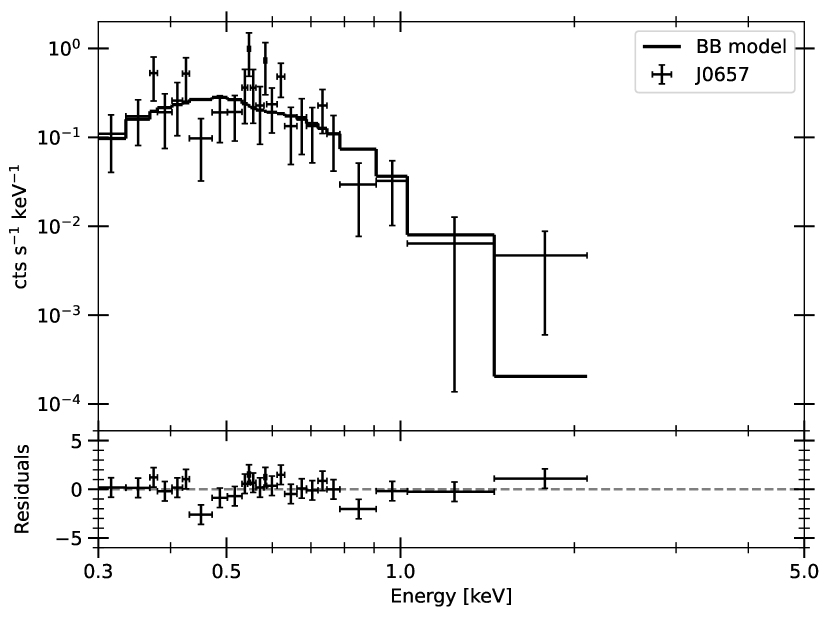
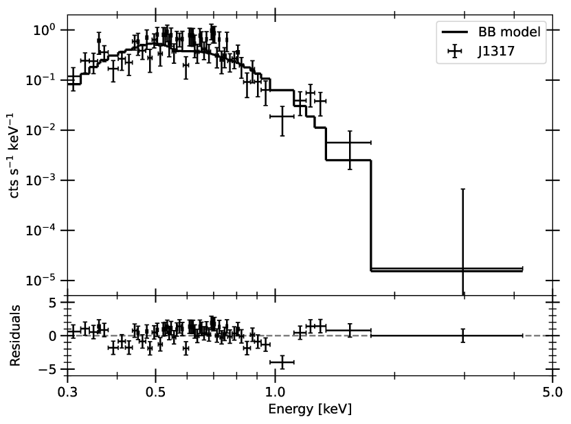
Figure 3: Stacked eRASS spectra for J0657 (top) and J1317 (bottom) along with the best-fit blackbody model (see Table 3). The spectra were rebinned for presentation purposes.

2.2 eRASS observations

The eRASS observations are carried out with eROSITA (Predehl et al., 2021), the primary instrument on board the SRG mission. eROSITA consists of seven Wolter-I X-ray telescopes (dubbed TM1, TM2,…, TM7; together referred to as the virtual telescope TM0). All telescopes are operated with a polyimide foil (the standard FILTER setup) to reduce contamination, while an aluminium filter is applied directly on the CCDs for TM 1, 2, 3, 4, and 6 (together dubbed virtual telescope TM8). For TM5 and 7 (dubbed TM9), only the polyimide foil contains a thin aluminium layer, making them more sensitive to soft X-rays. However, this configuration leads to a time-variable optical light leak (Predehl et al., 2021), which negatively affects the low energy calibration and performance. We list the available eROSITA observations for both candidates in Table 2.

To enable an analysis beyond the catalogue properties, we adopted the photon event lists produced with the most recent pipeline processing version c020 and analysed the data with the eSASS software package (version: eSASSusers_211214.0.4.2, Brunner et al., 2022). We filtered the observations for periods of low background with the flaregti task. The total net exposures are 598 s and 1397 s of ’good’ time (single visit times are presented in Table 2) for J0657 and J1317, respectively. We accepted all valid photon patterns (PATTERN$\leq$15) and excluded flagged or corrupted events, that is, those coming from bad pixels by applying FLAG=0xC000F000. We conducted a source detection run in the 0.2–10 keV band, as described in Brunner et al. (2022), with the goal of locating the target and nearby field sources via a maximum likelihood method of point spread function fitting. The output was used to create optimised source and background regions (Fig. 2) that we applied to generate the spectra via the srctool task. We then grouped the spectra with one count per spectral bin using the grppha (version: 3.1.0, Blackburn, 1995) task. The source detection results are in agreement with the catalogue values listed in Table 1. Nevertheless, the catalogue offers the advantage that systematic errors can be better taken into account. Namely, by comparing the full eRASS:4 catalogue to the ’astrometric selection’ from the GAIA DR3 qso_candidate catalogue (Gaia Collaboration et al., 2022a), a global systematic error of 0.6″ and an error scaling factor of 1.1 can be computed (see caption of Table 1). We present the single counts per visit in Table 2. Combining all telescopes and observations, 96 counts and 418 counts (0.2–5 keV band) were detected for J0657 and J1317.

2.3 Optical follow-up observations

We obtained deep optical imaging of J0657 in December 2021 and March 2022 (Table 2), using the Multi-Object Double Spectrograph 1 and 2 (MODS, Pogge et al., 2010) at LBT. Each MODS splits the incoming light into a blue and red channel, allowing the simultaneous observation in the $g$- and $r$-band. In each visit we obtained 4 $\times$ 50 s exposures with each MODS, leading to a total exposure time of 400 s in the $g$- and $r$-band. Unfortunately, the visit in March 2022 was affected by cirrus clouds, substantially increasing the sky background. For the image reduction, we used the most recent calibration images available for the respective visit. We first subtracted the bias from the science, dome, and sky flat frames and then divided the science images by a combined flat image created from the dome and sky flats.

The field of the INS candidate J1317 was observed with SALT in May 2022 (Table 2), using the Robert Stobie Spectrograph (RSS, Burgh et al., 2003; Kobulnicky et al., 2003) equipped with a fused silica clear filter. We obtained 40 $\times$ 60 s exposures in imaging mode and adopted the pipeline-processed images (version: 0.42). The pipeline corrects for gain and cross-talk, as well as the bias estimated from the overscan region; it also mosaics the CCDs. In the absence of a proper flat field correction, the images were divided by a median normalised background image, created using the photutils package (Bradley et al., 2022).

For both targets we derived the astrometric solution via the astrometry.net (Lang et al., 2010) code and aligned the single images via the wcsalign (Astropy Collaboration et al., 2013, 2018, 2022) method. The images were then added to reach the full depth.

3 Results

3.1 X-ray data analysis

3.1.1 Methodology

We adopted the Bayesian X-ray Analysis (BXA, Buchner et al., 2014) package in combination with XSPEC to fit models to the ’stacked’ (which combine events from all eRASS scans) TM0 spectra of both candidates. To account for the interstellar absorption in the direction of the X-ray source, we applied the tbabs model component and elemental abundances of Wilms et al. (2000). For the continuum, we tested a simple blackbody model (BB), a power law (PL), the emission spectrum of a hot, collisionally ionised, plasma (apec), and the neutron star atmosphere (NSA) model ( Pavlov et al., 1995; Zavlin et al., 1996). We left most parameters free to vary and fixed only the apec model abundance to the solar value. The parameter ranges were chosen to cover the physically acceptable range of parameter values. For parameters spanning multiple magnitudes (such as $N_{\rm H}$ ranging from $10^{18}$-$10^{23}$ cm^-2), we used log-uniform priors, whereas otherwise uniform priors were utilised.

We present the fit results for the different continuum model cases in Table 3. To compare the single fits, we also list the Bayesian evidence ($\log(Z)$), as well as Bayes factors (log(Z_BB/Z)) with respect to the BB result, and Akaike information criterion (AIC) values. The Bayesian evidence is also referred to as the model evidence and can be regarded as the probability that the given data can be produced by the model. The AIC describes the information loss between the process that created the observed data and the proposed model that is supposed to describe this process. In general, the model with the larger Bayesian evidence or smaller AIC value is to be preferred.

The spectra of the two INS candidates, folded with the best-fit blackbody models, are shown in Fig. 3. To estimate the overall fit quality, we present quantile-quantile and corner plots, displaying the parameter correlations and sample point distributions, in Fig. 4 and 5. The fit results do not significantly change if the TM8 or TM9 spectra are fitted instead. We conclude that the remaining calibration uncertainties of TM5 and TM7 do not significantly affect the estimated parameter values. This implies that statistical uncertainties dominate the spectra.

3.1.2 J0657

The Bayes factors and AIC values presented in Table 3 favour a BB model with $kT=108^{+15}_{-14}$ eV. Assuming a 1 kpc distance to the source, we find a $1.9^{+1.4}_{-0.7}$ km emission region radius. A PL fit results in worse log(Z) and AIC values and converges to a photon index of $6.5^{+0.9}_{-0.7}$, which is unreasonably steep for most AGN types (usual photon indices of 1.5–2.5, Ishibashi & Courvoisier, 2010), and $N_{\rm H}$ values exceeding the Galactic column density (presented in Table 1), which could support an extragalactic nature. We find the redshift parameter of the apec model to be consistent with zero and it was thence fixed. The fit resulted in a temperature $\sim 200$ eV and in $N_{\rm H}$ values below the Galactic column density, both in accordance with a stellar nature. The AIC and Bayesian evidence are, in comparison to the BB fit, still worse and we note that the quantile-quantile plot (Fig. 4) shows apec to systematically underpredict the source emission below energies of 0.7 keV.

We used the best-fit solutions of Table 3 to generate 200 BB, PL, and apec spectra and fitted the data with all three model types. The goal of the simulations is to evaluate the false-positive (the best-fit model is not the true model) and false-negative (the true model is rejected) rates, on the basis of the Bayes factors. The simulations show that the apec model is erroneously accepted in 1.5% of the cases for J0657, assuming that it emits as a blackbody. On the other hand, the small ($1.6$%) false-positive error of the blackbody disfavours apec as the underlying source spectrum. In the case of a BB nature, we never found a PL model to fit the spectrum better. Instead, we found a large false-negative rate for the steep PL spectrum, since a BB nature was favoured over the true PL in 65% of the cases. Dedicated, deeper observations, with better count statistics, are needed to discern between a BB and a PL model. As it can be seen for the case of J1317 (see Sect 3.1.3), a better exposed source spectrum can drastically reduce the false-negative rate and thereby also lead to generally worse PL fits.

We present the results of NSA fits in Table 3. We assumed a canonical NS with 12 km radius and a mass of 1.4 M_⊙. The fit quality is between those of the BB and apec fits; however, the NSA result converges to a 20–50% lower temperature, while the column density $N_{\rm H}$ exceeds the Galactic value (see Table 1). The difference in AIC and log(Z) are not sufficient to favour a particular magnetic field strength. The inferred distances are well in agreement with those of the known XDINS population.

We found no model combination (for example a BB+PL model that also accounts for non-thermal emission) that significantly improves the results of the single component models presented in Table 3. Nevertheless, one can estimate an upper limit for the non-thermal to thermal flux ratio, by fitting a BB+PL model with the PL photon index fixed to two. The fit converged to a BB component with $103^{+16}_{-14}$ eV, $N_{\rm H}$ of $6^{+5}_{-4}\times 10^{20}$ cm^-2, and an emission radius of $2.1^{+1.6}_{-0.9}$ km (at 1 kpc distance). The log(Z_BB/Z)=0.5 and AIC=65.3 indicate the fit to be of a similar quality to the single BB solution presented in Table 3. We computed $F_{\mathrm{PL}}/F_{\mathrm{BB}}\leq 56\%$ from the upper and lower $3\sigma$ power law and blackbody component flux limits located at $1.8\times 10^{-13}$ erg s^-1 cm^-2 and $3.2\times 10^{-13}$ erg s^-1 cm^-2 (0.2-10 keV).

tbabs $\times$ bbodyrad

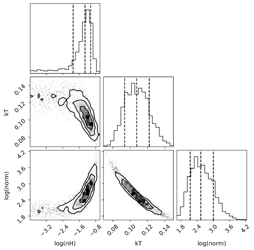
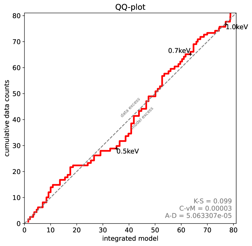
tbabs $\times$ apec

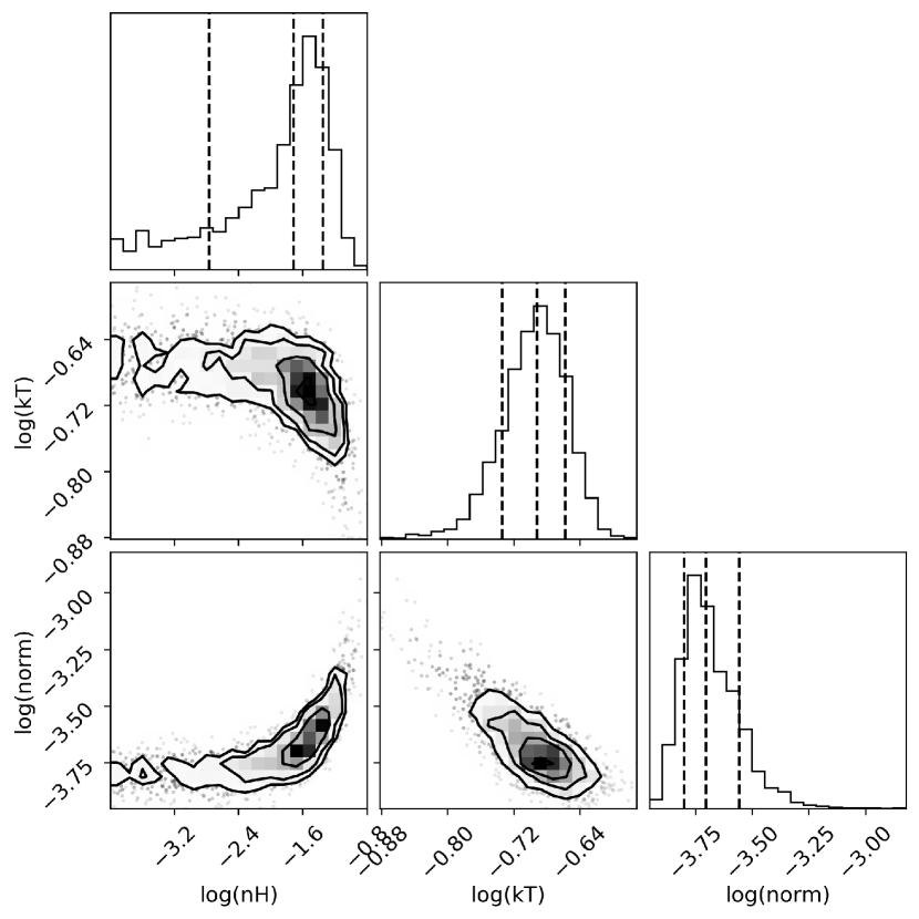
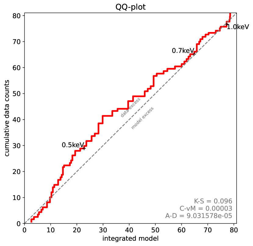
tbabs $\times$ powerlaw

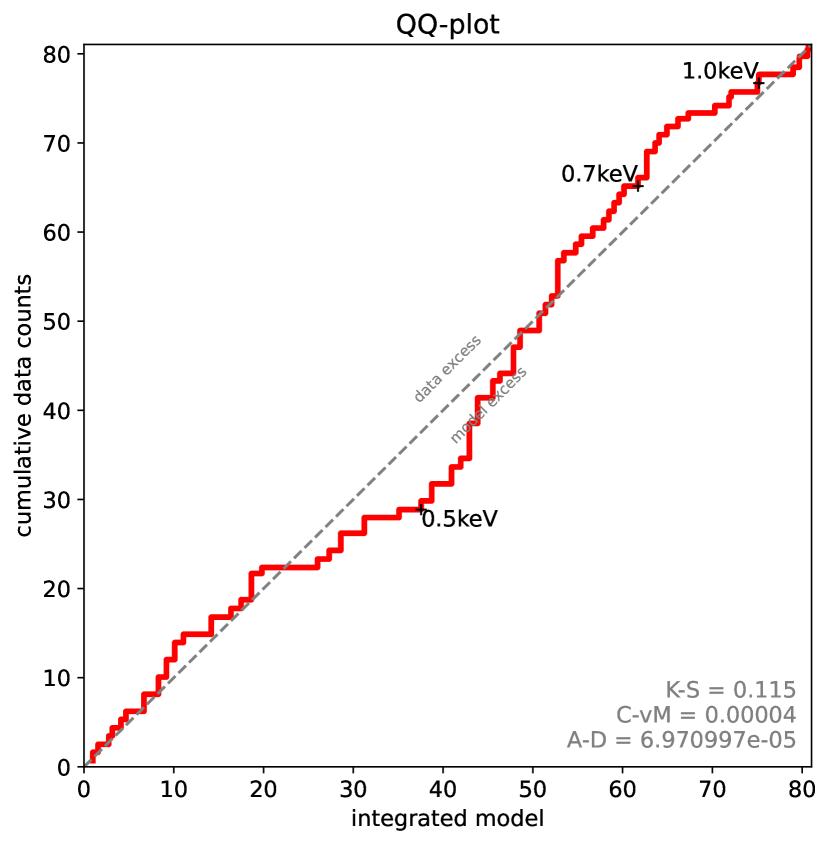
Figure 4: Diagnostic diagrams presenting the best-fit results for J0657 for absorbed blackbody, apec, and power law spectra. For each of the three models, the top row depicts corner plots presenting the parameter distribution and correlations based on the inferred sample of test points from the fit. The vertical dashed lines indicate the 16%, median, and 84% percentiles. The lower row contains quantile-quantile plots, comparing the cumulative sum of counts derived from the best-fitting model in comparison to the observed spectrum.

3.1.3 J1317

We found a BB with a temperature of $110^{+7}_{-7}$ eV to maximise the Bayesian evidence. The emission region radius at a 1 kpc distance computes to $3.0^{+0.9}_{-0.7}$ km. These values are in agreement with the expectation for an INS, but we found the fit to converge to a $N_{\rm H}$ value exceeding the Galactic limit (see Table 1). This is at odds with a Galactic INS interpretation, but could also hint towards a more complicated spectral shape. Contrarily, the AIC favours an apec fit that converges to a temperature of $281^{+15}_{-14}$ eV, coupled with a redshift of $0.170^{+0.016}_{-0.022}$ that might indicate an extragalactic nature. Interestingly, here the $N_{\rm H}$ converged to a result that is below the Galactic value and, as such, points towards the object being of Galactic origin. If one attempts to fix the redshift to zero, the fit quality worsens (log(Z_BB/Z)=13.87, AIC=153.67). A PL fit results in a photon index of $7.3^{+0.5}_{-0.5}$, which is again too steep for most known AGN types. The resulting log(Z) and AIC are clearly worse in comparison to the BB and apec models.

As for J0657, we simulated 200 spectra, using the best-fit solutions of Table 3 to estimate the false-positive and false-negative rates. Using the AIC as criterium, we find a large false-positive rate of 19% indicating apec to fit better, although we assumed BB emission for the source. Interestingly, for the same fits, the resulting Bayes factors never favoured the apec model over a BB fit. We conclude that the observed AIC, indicating apec to fit best, is likely a spurious result, although larger differences in AIC, as observed here, were found only for 1.5% of our simulations. On the other hand, the false-positive rate is very small (a true apec spectrum is never better described by a BB model). Thus, choosing the BB over the apec model seems to be robust.

We found no case where a BB spectrum was better fit by a PL than a BB model. Nevertheless, the false-positive rate of 8% – favouring a BB model, although the source has a PL nature – is still high. This value is much lower than the one observed for J0657, which we attribute to the higher number of counts in the J1317 case that allow for a better distinction between a BB and PL nature, but it is still difficult to reject an absorbed PL nature on the available fit alone.

The best-fit NSA model results, listed in Table 3, are generally worse than the BB and apec models. Comparing the Bayes factors, magnetised models seem to fit better and the distance estimates are in agreement with the known XDINS population. We again found the NSA model temperatures to be 25–50% of the BB temperatures, while the $N_{\rm H}$ is about twice the Galactic value, which is at odds with a Galactic nature of the source.

Similarly to J0657, we found no multi-component models that significantly improve the fits in comparison to the single component models shown in Table 3. A BB+PL fit, with the photon index fixed to two, is worse in quality, but it converges to BB parameter values very similar to the single BB result (log(Z_BB/Z)=1.0, AIC=129.5, $N_{\rm H}=10.7^{+4.0}_{-2.7}\times 10^{20}$ cm^-2, $kT=108^{+8}_{-8}$ eV). The fit results in an upper 3$\sigma$ PL flux limit of $1.3\times 10^{-13}$ erg s^-1 cm^-2 and a lower 3$\sigma$ BB flux limit of $1.1\times 10^{-12}$ erg s^-1 cm^-2 (0.2–10 keV). Thus, we found $F_{\mathrm{PL}}/F_{\mathrm{BB}}\leq 12\%$.

tbabs $\times$ bbodyrad

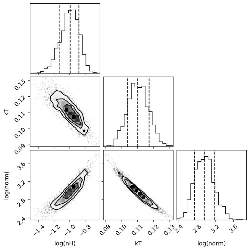
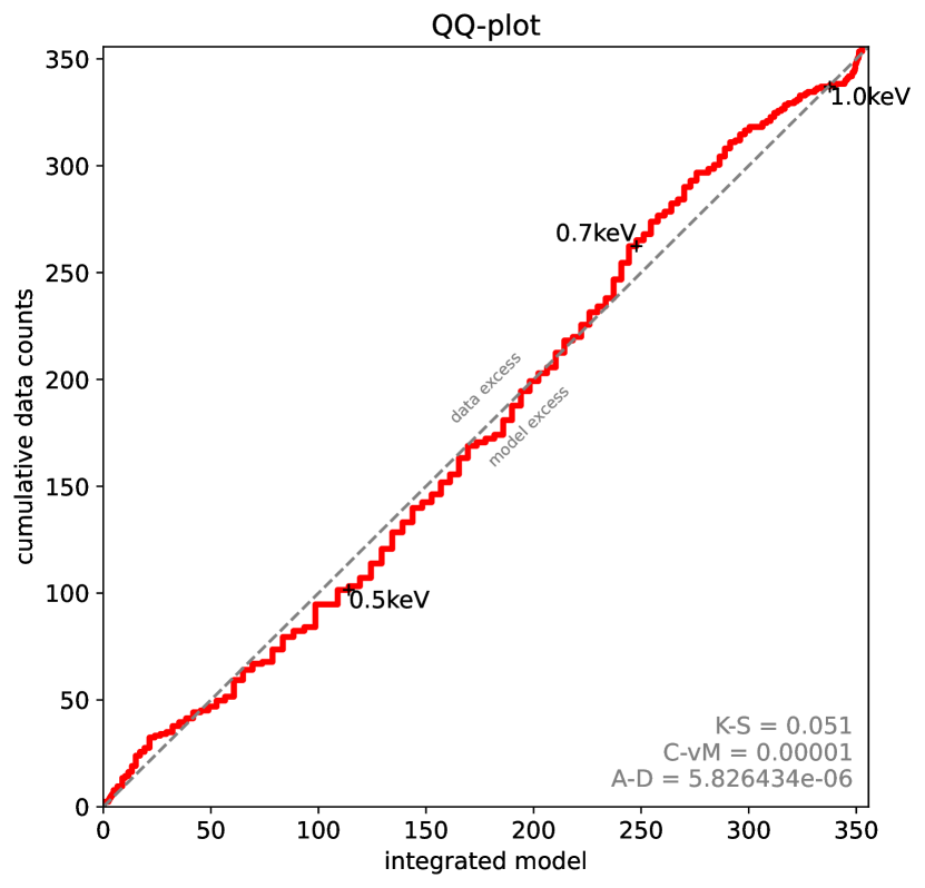
tbabs $\times$ apec

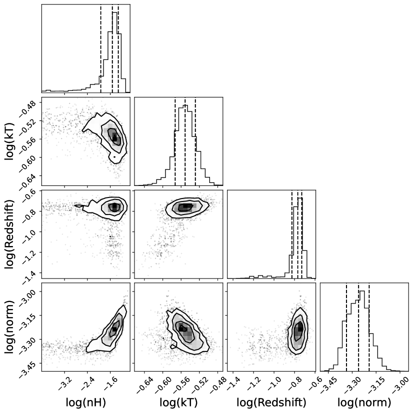
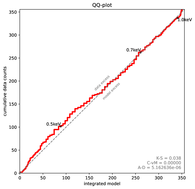
tbabs $\times$ powerlaw

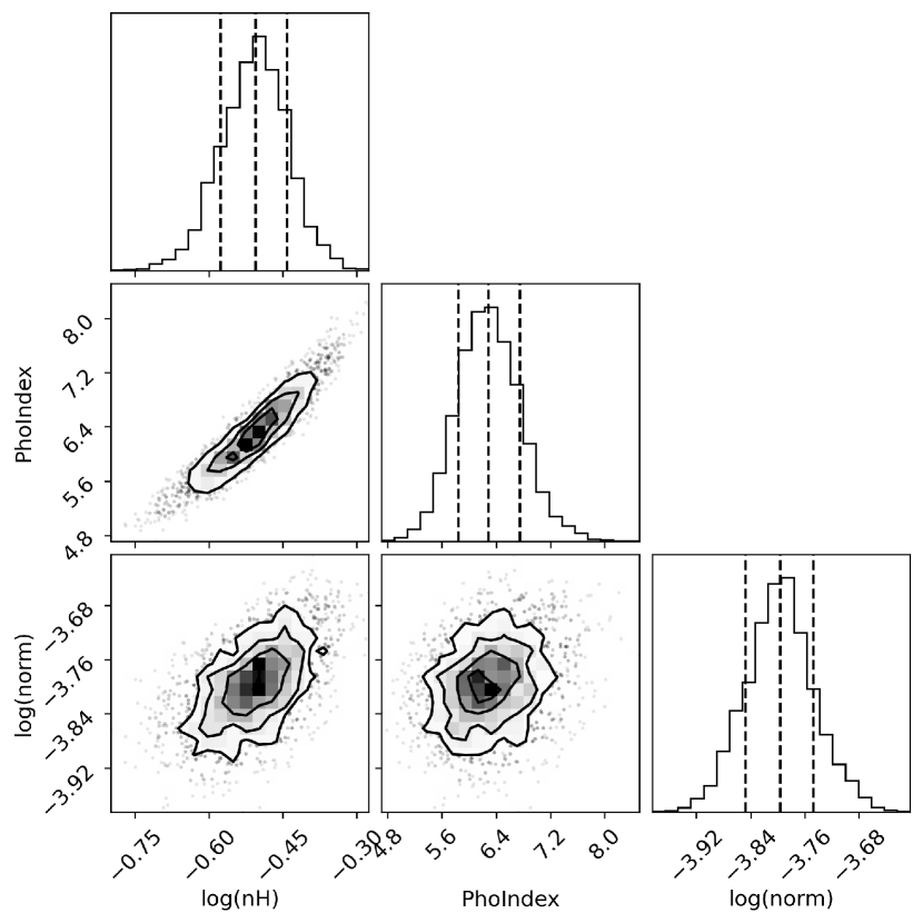
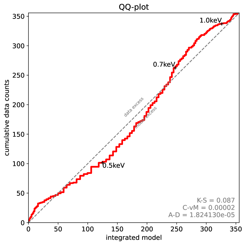
Figure 5: Diagnostic diagrams presenting the best-fit results for J1317 for absorbed blackbody, apec, and power law spectra. For each of the three models, the top row depicts corner plots presenting the parameter distribution and correlations based on the inferred sample of test points from the fit. The vertical dashed lines indicate the 16%, median, and 84% percentiles. The lower row contains quantile-quantile plots, comparing the cumulative sum of counts derived from the best-fitting model in comparison to the observed spectrum.

Table 4: Simultaneous blackbody fit results of the single eRASS spectra.

J0657
eRASS	$kT$	Radius	Absorbed flux
	[eV]	[km]	[$10^{-13}$ erg s-1 cm-2]
1	$85^{+16}_{-13}$	$3.7^{+2.4}_{-1.5}$	$2.5^{+0.8}_{-0.6}$
2	$125^{+17}_{-18}$	$1.3^{+0.7}_{-0.4}$	$2.6^{+0.8}_{-0.7}$
3	$94^{+15}_{-12}$	$3.1^{+1.7}_{-1.1}$	$3.1^{+0.7}_{-0.7}$
4	$119^{+19}_{-16}$	$1.4^{+0.8}_{-0.5}$	$2.0^{+0.6}_{-0.5}$
J1317
eRASS	$kT$	Radius	Absorbed flux
	[eV]	[km]	[$10^{-13}$ erg s-1 cm-2]
1	$104^{+7}_{-7}$	$3.7^{+0.9}_{-0.7}$	$4.8^{+0.5}_{-0.5}$
2	$113^{+9}_{-8}$	$2.8^{+0.7}_{-0.6}$	$4.4^{+0.6}_{-0.5}$
3	$115^{+11}_{-9}$	$2.8^{+0.8}_{-0.7}$	$4.7^{+0.8}_{-0.7}$
4	$110^{+10}_{-9}$	$3.0^{+0.9}_{-0.7}$	$4.3^{+0.6}_{-0.6}$
5	$111^{+11}_{-10}$	$2.6^{+0.9}_{-0.7}$	$3.5^{+0.6}_{-0.6}$

3.2 Variability and timing

The available eROSITA data, spanning multiple epochs (see Table 2), allow one to check for flux variations. To this end, we conducted simultaneous fits to the single eRASS spectra with an absorbed blackbody component, fixing the $N_{\rm H}$ to the value obtained from the fits to the stacked data, but leaving the normalisation and effective temperature free to vary between the different eRASS visits. The result is shown in Table 4. There are no hints towards a significant variation for either of the two candidates since the flux values are in agreement with each other within 1–2$\sigma$. Variations of this size were also observed for the known XDINSs and they can be attributed to low-count statistics (see Appendix B in Pires et al. (2022) for a more detailed discussion). For J1317, there is a source, 27″ away from the eRASS position, in the second ROSAT all-sky survey source catalogue (Boller et al., 2016). Considering the $1\sigma$ positional uncertainty of 20″, the identification seems robust, mostly since there are no similarly bright eRASS sources in a 5′ radius around J1317. We used the sample point distribution of the best-fit BB model from Table 3 to simulate the expected ROSAT count rate with XSPEC. We found a count rate of $2.9^{+1.5}_{-0.8}\times 10^{-2}$ s^-1 (0.1–2.4 keV) which is in agreement with the ROSAT catalogue count rate of $6.5(1.8)\times 10^{-2}$ s^-1 (0.1–2.4 keV) within 2$\sigma$. J0657, on the other hand, was not detected by ROSAT. From five ROSAT sources within 45′ of the eROSITA position, we determined that ROSAT was pointed for about 430 s in the direction of J0657, which would result in an expected ROSAT count rate of $1.9^{+1.2}_{-1.0}\times 10^{-2}$ s^-1 (0.1–2.4 keV). This is at the detection limit, as can be seen from the lower panel in Fig. 8 of Boller et al. (2016).

As the sources were observed in scanning mode, a search for pulsations is not feasible. For J0657, only about 17–25 photons (0.2–5.0 keV) are detected in each visit (Table 2). The largest photon count (105 photons) was achieved for J1317 during eRASS1. We applied a Z${}^{2}_{m}$ periodicity search (Buccheri et al., 1983) and did not find any significant pulsations. For pulsations within $P=100$ ms – $20$ s (using events within 0.2–2.0 keV and $1.3\times 10^{6}$ independent trials), this provides a non-constraining 3$\sigma$ upper limit for the pulsed fraction of 87%.

3.3 Optical imaging

We applied the SExtractor software (Bertin & Arnouts, 1996), to search for optical sources near the position of our INS candidates. The closest optical objects were detected 10$\sigma$ ($13$″ distance, J0657) and 6.7$\sigma$ ($6$″ distance, J1317) away from the respective X-ray sources’ sky position. We find no viable optical counterpart in any of the INS fields (see images in Fig. 6). In order to estimate the resulting X-ray-to-optical flux ratio limits, we cross calibrated the flux, measured in an optimised aperture from the SExtractor run, against the Pan-STARRS DR1 (Chambers et al., 2016) $g$- and $r$-band (J0657) or the GAIA DR3 (Gaia Collaboration et al., 2022b) $g$-band (J1317). The X-ray-to-optical flux ratios were computed based on the equation for the magnitude limit of a point source in an optimal Gaussian aperture (assuming a 5$\sigma$ detection limit). We determined the magnitude limit to be at magnitude 25.7 and 25.5 in the Pan-STARRS $g$- and $r$-band (J0657) and magnitude 25 in the GAIA $g$-band (J1317). The estimated photometric parameters and flux ratios are listed in Table 5. We compare the resulting absorbed X-ray-to-optical flux ratios to those of the most prevalent contaminants in Fig. 7. The candidates’ X-ray-to-optical flux ratio values are almost a magnitude larger than those of the contaminants. Taking the interstellar absorption into account and using the Predehl & Schmidt law (Predehl & Schmitt, 1995), as well as the reddening coefficients from Cardelli et al. (1989), we derived unabsorbed X-ray-to-optical flux ratio limits ranging from 1000–2000.

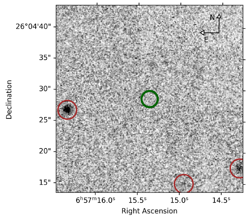
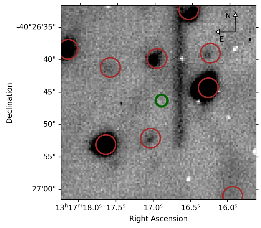
Figure 6: LBT MODS $r$-band image depicting J0657 (left) and SALT RSS image obtained for J1317 (right). The candidate position is indicated by green circles, with the radius equivalent to the 1$\sigma$ confidence regions listed in Table 1. All nearby field sources, detected from a SExtractor run, are indicated with brown circles.

Table 5: Photometric parameters and magnitude limits.

Parameter	$g$-Band	$r$-Band	$g$-Band
	(J0657)	(J0657)	(J1317)
Magnitude Zeropoint	33.7	33.8	37.3
$\sigma_{\mathrm{sky}}$	25.1	35.4	2083
FWHM (px)	10.7	10.7	6.9
FWHM (″)	1.29	1.31	1.75
5$\sigma$ mag. limit	25.65	25.46	24.97
abs. $f_{\mathrm{X}}/f_{\mathrm{opt}}$	1023	859	1167
unabs. $f_{\mathrm{X}}/f_{\mathrm{opt}}$	1392	1259	2111

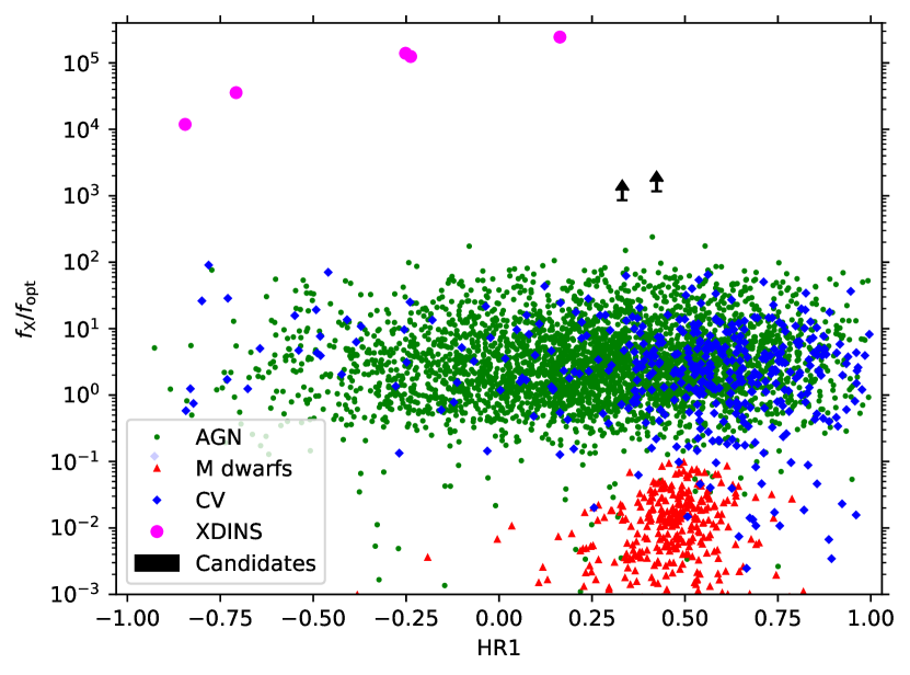
Figure 7: Candidate X-ray-to-optical flux ratio limits (black) are compared to those of the known XDINS population on the German eROSITA sky (magenta, optical flux values are based on Kaplan et al., 2011) and the most prevalent contaminants of our search, namely M dwarfs (red, taken from Magaudda et al., 2022), cataclysmic variables (blue, selected from the Ritter and Kolb catalogue (Ritter & Kolb, 2003) and the open CV catalogue by Guillochon et al. 2017), and AGN (green, taken from Liu et al., 2022).

4 Discussion and outlook

We report the discovery of two predominantly thermal INS candidates from eRASS. Both targets were followed up on in the optical with LBT and SALT, revealing no counterparts brighter than magnitude 25. The present optical limits confidently exclude more ordinary classes of X-ray emitters than an INS (Schwope et al., 1999, and see Fig. 7). The spectra of both sources are well described by simple blackbodies with $kT\sim 110$ eV, which is well in agreement for a cooling INS. The best-fit BB models are absorbed by column densities of $5-10\times 10^{20}$ cm^-2, although the estimated $N_{\rm H}$ exceeds the Galactic value (see Table 1) in the case of J1317. This suggests a more complex spectral shape, although we did not find a multi-component model to fit better than a single blackbody. Neutron star atmosphere models with temperatures of 30–50 eV and short distances of a few hundred parsecs do not reach the fit quality of a single BB component model. For both candidates, the best-fit column density is a factor of one to two in excess of the Galactic value in the direction of the sources.

Other single-component spectral models (power law, apec) describe the spectra in some instances equally well. In particular, the current spectra do not allow one to discern between a strongly absorbed power law or blackbody nature. The photon indices of the best-fit power law models in Table 3 are consistent with those of narrow-line Seyfert I galaxies observed in the eROSITA footprint (Grünwald et al., 2022). However, their optical counterparts are expected to be at least 1.5 magnitudes brighter than the present optical limits we derived for our INS candidates. Likewise, a star in our Galaxy, which is a viable solution for the INS candidate J0657 on the basis of its best-fit apec model, should be brighter than magnitude 16; this is again in stark contrast with our follow-up results. The lower temperature of the best-fit blackbody and apec models also disfavour a cataclysmic variable (CV) nature. While high-energy emission (above 1.5 keV) is to be expected in most CV types (Mukai, 2017), we see no indication for it in the spectra of either INS candidate (see Fig. 3). Finally, for both sources we find no significant variability in either flux or spectral state over the two-year time span covered by the eROSITA data. Interestingly, the source J1317, possibly detected by ROSAT, may be stable over even longer timescales (30 yr). Additional observations are not available since none of the candidates have been targeted or serendipitously detected with XMM-Newton, Chandra, or Swift in the past. We searched the radio catalogues provided in the Vizier catalogue access tool (Ochsenbein et al., 2000), but did not find any counterparts close to the X-ray sky positions of either candidate.

To put both candidates in the context of other thermally emitting INSs, we applied the Stefan–Boltzmann law to compute luminosity estimates. Since there are no constraints on the distance, we assumed a broad range of trial distances ranging from 0.1–5 kpc. The resulting $1\sigma$ regions in the radius-luminosity diagram are marked in Fig. 8, along with archival cooling INS and NS hot spots collected in Potekhin et al. (2020). For small distances (¡ 0.3 kpc), the luminosity is in agreement with a neutron star hot spot, at intermediate distances (0.3–3 kpc) the candidates could be intermediately aged rotation-powered pulsars (indicated by the ordinary pulsars in the diagram) or XDINSs, while larger distances are in agreement with a CCO-like nature or ordinary and high-B pulsars. Based on the Galactic position and assuming the same trial distance range, the candidates are located 60–1000 pc (J0657) and 110–1840 pc (J1317) above the Galactic disc. Constraints on the NS age can be derived under the assumption that the candidates formed close to the Galactic plane. From the known INS population, we know that most objects possess velocities below 1000 km s^-1 (Hobbs et al., 2005). Based on this upper value, we computed lower age limits of 65–650 kyr (J0657) and 110–1100 kyr (J1317). This is in agreement with an intermediate rotation-powered pulsar or XDINS, but is at odds with a CCO nature. The reasoning is that in accordance with Fig. 8, weakly magnetised INSs would possess the largest distances, but this results in ages that exceed those observed for the young CCOs (typical ages of a few hundred to a few thousand years, see Mayer & Becker, 2021, and references therein). We found magneto-thermal evolution models, taking the effects of magnetic field decay into account, as for example described in Viganò et al. (2013), to give similar age estimates. We compared the luminosities to Fig. 11 in the same publication and found that the observed luminosities of $10^{31}-10^{33}$ erg s^-1 imply ages on the 100,000 yr to a few million year timescale.

Most INSs of the classes considered above possess mixed X-ray spectra that contain both thermal and non-thermal emission components. In Sect. 3.1.2 and 3.1.3, we estimated the upper non-thermal to thermal flux ratio limit based on the results of a BB+PL fit and found those values to be at 56% and 12% for J0657 and J1317, respectively. These ratios do not exclude the existence of a non-thermal component, since smaller ratios have also been observed for rotation-powered pulsars. For example, the rotation-powered pulsar PSR~B0656+14 has a ratio of 0.3% (De Luca et al., 2005), such that the apparent absence of non-thermal emission for our candidates does not allow for the possible nature to be constrained. Additional follow-up is necessary to achieve this goal.

Both candidates conform well with an INS interpretation, but the exact nature cannot be determined on the available data alone. This may change in the near future since both candidates will be observed with XMM-Newton and NICER in the upcoming cycles, as part of a programme to further follow up on the most promising INS candidates from eRASS. In particular, the observations will improve the localisation and spectral parameters, as well as allow one to search for pulsations down to pulsed fractions of 5%.

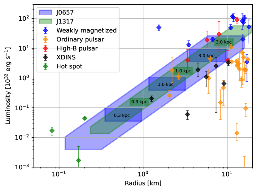
Figure 8: For J0657 (blue) and J1317 (green), we show the 1$\sigma$ confidence region distribution in luminosity and emission radius space, as it can be derived from the best-fit BB model depicted in Table 3. The rectangles indicate the 1$\sigma$ confidence region at certain distances. For the computation via the Stefan-Boltzmann law, we assumed varying test distances ranging from 0.1–5 kpc. The radius-luminosity positions of thermal emission components observed in archival INSs are marked as well. The values and object descriptions were taken from Potekhin et al. (2020).