Computing the optimal transport density: a FEM approach
Abstract.
The optimal transport density is the unique solution of the Monge-Kantorovich equations. It has been recently characterized also as the unique minimizer of the -transport energy functional . In the present work we develop and we prove convergence of a numerical approximation scheme for Our approach relies upon the combination of a FEM-inspired variational approximation of with a minimization algorithm based on a gradient flow method.
Key words and phrases:
Monge-Kantorovich Equations, Optimal Transport, Gradient Flow, Convex Optimization with Positivity Constraints, Łojasiewicz Inequality1991 Mathematics Subject Classification:
68Q25 68R10 68U051. Introduction
1.1. optimal transport
Optimal transport is the mathematical problem modeling the quest for an optimal strategy for moving a mass displacement of a material to a target distribution. Apart from the original motivation of soil dragging [27], optimal transport finds a large variety of applications, e.g, metrics in probability theory, smoothing in image processing, baricentric interpolation and many others (see for instance [30, 31] and references therein). The modern formulation of optimal transport is due to Kantorovich, see [23], and can be stated as follows. Let be two Borel measures defined on with finite equal masses. Let be a Borel function. Find a non-negative Borel Measure on (termed optimal transport plan) realizing the following infimum
| (1.1) |
under the constraints
Existence of such an optimal transport plan is guaranteed by mild assumptions on , e.g., lower semicontinuity and boundedness from below.
In this paper we focus on the case, i.e., we assume . Also, we will work under the (classical) further assumption of , for a given zero-mean function In this setting not only the problem (1.1) admits a unique optimal transport plan, also such a plan is defined by an optimal transport map, i.e., a Borel function realizing the minimum in the Monge formulation of optimal transport, i.e.
where is the push-forward measure.
The aim of the present work is to study an approximation algorithm for the solution of the -optimal transport. While the numerical solution of optimal transport has been tackled in several previous works (see e.g. [3, 5, 11] for recent contributions), schemes for the case are sparser. Typical methods for the numerical solution of this latter problem are based on the entropic regularization of the linear programming problem associated to the Kantorovich formulation and augmented Lagrangian methods, or on the reformulation of the problem in Beckmann form [13, 4, 24, 28].
In our work, we take inspiration from the work of [16, 17], where a numerical solver for the PDE based formulation of this problem was proposed. The PDE formulation of the -optimal transport originated in [15] who showed that the -optimal transport map can be constructed starting from the optimal transport density, i.e., the unique solution of the so-called Monge-Kantorovich equations
| (1.2) |
where is a bounded convex domain compactly containing . The approximation of the solution of (1.2) is a very difficult task. Indeed, the coupling of the linear PDE with the constraints on the gradient of give rise to a highly nonlinear problem with inequality constraints in the variable . Also, due to the nonlinearity of (1.2), it is not a priori clear weather (and in which sense) the solution of certain discretized version of (1.2) would converge to the solution of (1.2).
The fundamental advance introduced in [16, 17] is to address the numerical solution of the variational reformulation of the Monge-Kantorovich equation presented by [9] and solve the related optimization problem by a gradient method. In these works, the authors introduce a Lyapunov-candidate functional and conjecture the existence of a continuous time gradient flow whose asymptotic solution coincides with the optimal transport density. Relying on this conjecture, the authors propose an efficient numerical scheme for the integration of the flow based on the explicit Euler discretization of the gradient flow and the finite element approximation of the relevant integrals. We would like to note that this approach is based on the formulation of a minimization problem and its subsequent discretization. The resolution of the conjecture has been hampered by the lack of results related to existence and uniqueness of the gradient flow and its trajectories, an outcome of the setup of the minimization problem in non-separable infinite dimensional spaces. As a consequence, no theoretical convergence of the above numerical scheme have been obtained and only experimental results are available to justify this approach.
The aim of the present work is to fill this gap and develop the complete theoretical convergence analysis of the FEM-based numerical method for the approximation of the optimal transport density. The properties of the studied discretization naturally suggest that, in contrast with the explicit nature of the method proposed in [16, 17], implicit Euler and Newton schemes must combine effectively to provide a super-linearly convergent method for the solution of the -optimal transport problem.
The strategy that allows the completion of our goal can be summarized as follows. Rather than tackling the proof of the conjecture, we reformulate the problem by first discretizing the relevant functional and then defining a gradient flow in a finite-dimensional setting. This discretize-minimize approach, opposite to the minimize-discretize suggested in [17], defines a sequence of finite-dimensional approximations of the above mentioned Lyapunov-candidate functional that are designed to provide a sequence of minimizers that converge towards the optimal transport density. The minimization step of the proposed strategy exploits the real analyticity of these approximations to derive a well-posed and smooth gradient flow that converges exponentially towards the sought solution under mild hypotheses. Within this proposed framework, we are able to prove the convergence of the proposed algorithm towards the optimal transport density, to provide a sharp convergence rate estimate, and to design robust and efficient stopping criteria. The final scheme includes an adaptive time-stepping strategy that allows the use of a geometrically increasing sequence of time-step sizes leading to super-exponential convergence towards the minimizer, thus drastically improving the computational performance with respect to previous work.
1.2. Our study
Our starting point is the variational characterization of the transport density proposed in [18] and the following definition of a -transport energy:
Definition 1.1 (-Transport energy [18]).
Let be a bounded Lipschitz domain of and let be such that and . We denote by the transport energy functional defined by
| (1.3) |
and we consider the following variational problem:
Problem 1.2 (Minimization of the transport energy).
Given as above, find such that
Here and throughout the paper we denote by the space of Borel signed measures on by the non-negative Borel measures, and by the space of Borel probability measures. In addition, our work relies on the following fundamental property, see [18, Prop. 2.1].
Proposition 1.3.
Problem 1.2 has an unique solution which is an absolutely continuous measure with
We start by introducing a double indexed sequence of functionals corresponding to the restriction of to certain finite element spaces and on which we approximate and , respectively (Section 2). We consider the diagonal sequence and we show that its -limit is , the lower semicontinuous regularization of the restriction of to a dense subspace. Nevertheless, we prove in Theorem 2.6 that
moreover any sequence of minimizers of converges to the unique minimizer of in the weak∗ topology of measures, i.e.,
This result motivates the study of the numerical solution of the problems
Next (Section 3), we study conditions that ensure well-posedness and well-conditioning of these discrete minimum problems. In particular we show in Proposition 3.2 that under the Hypothesis 3.1 there exists a unique minimizer of for any , i.e., the discretized minimum problems are well-posed. Under a slightly different assumption, namely Hypothesis 3.3, we prove that such problems are also well-conditioned, see Proposition 3.4.
The following step (Section 4) is to prove global existence, uniqueness, and regularity of the following two gradient flows
Namely the gradient flow equation (4.1) for the function which is obtained from with the use of canonical coordinates on , and the gradient flow equation (4.8) for the function which is obtained from by composition with the coordinate square map (i.e., ). In particular, in Theorem 4.1, we prove that any trajectory of the first flow is converging to a global minimizer of , while we prove in Theorem 4.3 that any trajectory of the latter is converging to a local minimizer of : applying the coordinate square map we recover a global minimizer of
The definition and study of the optimization algorithms for and derived from the time discretization of the two flows above conclude our theoretical contributions (Section 5). In the first case one needs to take into account the non-negativity constraint on , so an explicit time discretization seems to be necessary. Thus the gradient flow (4.1) of can be integrated by the so-called projected forward Euler scheme, which can be solved by Algorithm 1. On the contrary, the gradient flow of is defined on , and this makes feasible the use of an implicit scheme: our choice is indeed the backward Euler scheme coupled with the (zero finding) Newton’s Method with a prescribed initial guess. We focus on the latter scheme, both because it is more promising from a numerical point of view, e.g., there are no inequality constraints, and because -roughly speaking- the higher smoothness of the continuous time trajectories should provide faster convergence. We prove in Theorem 5.1 the consistency of this scheme, i.e., the Newton’s Method converges at each time step and the sequence of the backward Euler iterates converges to a local minimizer of Then we define Algorithm 2 by choosing a particular a posteriori stopping criterion that allows us to prove a stability estimate (see Proposition 5.2). We finally prove in Theorem 5.3 the convergence of Algorithm 2 and give in Proposition 5.5 a sharp estimate of the rate of such convergence. The combination of Theorem 2.6, Theorem 5.1, and Theorem 5.3 leads to (see Corollary 5.4)
where we denoted by the limit in the weak∗ topology of measures, and by the embedding deriving from the FEM coordinates.
2. -convergence of finite elements discretization
2.1. Finite elements discretization of
We want to introduce and study a sequence of functionals that provides a well-designed sequence of approximations of for minimization purposes. In order to be termed ”well designed” the sequence needs to fulfill certain desirable properties as preserving the convexity of , having (at each stage) finite dimensional domain, possibly being smooth, and being relatively easy to be evaluated at any given point. In addition, since we are interested in the minimization of , we need to be able to prove that any sequence of minimizers converges to the minimizer of . We introduce a suitable FEM-based sequence of approximations of in the present subsection and we will prove its convergence in the next subsection.
Let us remark that, as pointed out in [15] and in [18], the role of is not relevant in our work as long as it is an open bounded convex set compactly containing the set where stands for the convex envelope operator and for the support. Therefore, possibly up to translations an dilations, we can assume a very convenient choice for our purposes. This choice prevents the need of the analysis of the so-called geometric error that occurs when considering approximations of by unions of simplices which are the elements of choice in our approach.
First, we pick a sequence of nested triangulations of indexed over and obtained by uniform refinements. Let us denote by the space of continuous real functions such that is an affine function for any Similarly, is the space of functions such that is equivalent to a constant function for any Then we can consider the finite dimensional function spaces
and denote by the non-negative cone in , i.e.,
Second, we pick a monotone sequence such that as .
We can now introduce a double sequence of approximations of the functional that is a good candidate for the variational approximation of Notice that we can re-write , for notational convenience, as
where and
Then we define
| (2.1) |
where, for any , we set
| (2.2) |
Remark 2.1.
We would like to stress here that the use of the two indices and is dictated by notational convenience. Indeed, as we will see in the next sections, the principal object of our study will be the diagonal sequence , and in this case it produces the wanted combination of meshes and spaces for and for .
In our work we will use the functionals
| (2.3) | ||||
| (2.4) | ||||
| (2.5) |
where stands for the lower semicontinuous envelope with respect to the weak∗ topology of measures, i.e.,
Here and throughout the paper, when we consider measures that are absolutely continuous with respect to the Lebesgue measure, we use (by a slight abuse of notation) the same symbol both for the density of a measure and the measure itself. Accordingly, denotes the measure
Note that the definition of the functionals is taylored to the need of treating the convergence of minimizers. A more explicit representation is obtained by means of the linear isomorphism mapping onto . Precisely, for any we can define
and, for any , we denote by the vector
| (2.6) |
Analogously, given a basis of (where ), we can identify any function with its coordinates , where
Given and , we us introduce the matrices
| (2.7) |
and, for any , the matrix-valued function (the stiffness matrix)
| (2.8) |
We extend such a definition to each , a.e., by setting
| (2.9) |
We also denote by the load vector , where ,
Remark 2.2.
We remark that, in order to distinguish indeces denoting an element of a sequence from indeces refering to a component of a vector, we use the following convention: in the latter instance we add parentheses to the index, e.g., given the sequence of vectors , we denote by the -th component of the vector .
It is worth pointing out that the operation of taking the supremum of among (used in the definition of given in eq. (2.1)) corresponds to calculating the -finite element approximation of the solution of
| (2.10) |
More precisely, given , we have
| (2.11) |
where is the unique element of such that
| (2.12) |
in other words,
| (2.13) |
In view of this we set , that is
| (2.14) |
where we denoted by the area vector
Let us consider the coordinate square map defined by setting
| (2.15) |
We can introduce the functional
Notice that the image under the map of any local minimizer of on is a local minimizer of on Moreover is a global minimizer of on due to the convexity of the objective.
The next proposition collects some properties of and that will be useful later on.
Proposition 2.3 (Differential properties of and ).
For any the functional is convex on and real analytic on
The functional is real analytic on In particular, and any such that , we have
| (2.16) | |||
| (2.17) | |||
| (2.18) | |||
| (2.19) |
where is defined in (2.13). The convex subdifferential of can be characterized on the closure of by
| (2.20) |
The minimal norm subdifferential satisfies
| (2.21) |
Proof.
The convexity of is elementary because it is defined as the supremum of affine functionals and the composition with clearly preserves such a property.
Notice that is a positive definite (and thus invertible) symmetric matrix for any and linearly depending on . Since the matrix inversion is a real analytic operation the function is real analytic on
Using and (2.13), we obtain eq. 2.16 and similarly eq. 2.18. By the chain rule we obtain eq. 2.17 and eq. 2.19. Notice that is the restriction to the non-negative cone of a (similarly defined) real analytic function defined on For small enough, using the definition of convex subdifferential, we can write
Dividing by and passing to the limit as we get
Thus (2.20) follows. Equation (2.21) is immediately obtained by minimizing the norm over this set. ∎
Corollary 2.4.
Any critical point for (i.e., ) is a global minimizer for . If is a local minimizer for , then is a global minimizer for .
Corollary 2.5 (Discrete Monge-Kantorovich equations).
For any there exists at least one minimizer of on We have if and only if there exists a (unique) such that the following equations hold true
| (2.22) |
2.2. Convergence of minimizers of to
The aim of the present section is to prove the following result.
Theorem 2.6.
Let Then
| (2.23) |
the optimal transport density of the Monge-Kantorovich equations.
Remark 2.7.
We choose to focus our study on the ”diagonal sequence” of functionals to simplify our notation and avoid few technicalities in our proofs. However, the reader can easily check that our results still hold for any subsequence such that and are non-decreasing diverging sequences.
-convergence is the main tool that we are to going to use in the proof of Theorem 2.6, and, to fix our notation, we recall in the following paragraphs the needed definitions and properties. Let be a topological space and, for any , let us denote by the filter of the neighborhoods of Let We define
If there exists a function such that
| (2.24) |
then we say that -converges to with respect to the topology and we write or Our main interest on this notion of convergence is given by the following property (cfr. for instance [14, Cor. 7.20]). Assume that and is a minimizer of . Then any cluster point of is a minimizer of and If moreover converges to in the topology then
A useful property of -convergence is that it is well-behaving under monotone limits of lower semicontinuous functionals, [14, Prop. 5.4, Rem. 5.5, Prop. 5.7]. Indeed we can prove a preliminary result exploiting the two monotonicities of the double sequence
Proposition 2.8.
Proof.
Equation 2.25 follows easily observing that is an increasing sequence of lower semicontinuous functionals and hence its -limit coincides with its point-wise limit.
To prove the second statement, we first notice that
| (2.27) |
The first equality follows by definition. For the second equality we proceed as follows. We first notice that, if then there exists such that, for any , and for all Then we can write
If we pick the lower semicontinuous regularization of eq. 2.27 we get
| (2.28) |
Note that, since iterated operators commute, using eq. 2.25 we have
| (2.29) |
On the other hand, using again the monotonicity we have
| (2.30) | ||||
| (2.31) |
The combination of equations (2.28), (2.29), (2.30), and (2.31) leads to
Since the iterated Gamma-limits exist and coincide, also the diagonal Gamma-limit exists and it is equal to the iterated limits, i.e., the first equality of (2.26) holds true. ∎
The above proven -convergence ensures that any cluster point of a sequence of minimizers of is a minimizer of but it does not imply by itself the existence of the cluster point. However, we are able to show that indeed this cluster point does exist.
Proposition 2.9.
For any , let Then is pre-compact in the weak∗ topology of measures. Any cluster point of lies in and we can extract a subsequence such that
| (2.32) |
Proof.
Notice that, denoting by the -dimensional Lebesgue measure,
| (2.33) |
Let be the solution of (2.12) with Notice that, denoting by the Poincaré constant of and using (2.11), we have
Here we used the Poincaré Inequality and the weak formulation (2.10). It follows that the sequence has bounded mass:
Thus we can extract a weak∗ converging subsequence, and the limit is a minimizer of the -limit functional (i.e., of by 2.25) due to basic properties of -limits, cfr. e.g., [14, Cor. 7.20]. ∎
The proof of Theorem 2.6 essentially relies on the uniqueness and the regularity of the optimal transport density Indeed, under our assumptions, the optimal transport density is uniquely determined and it is an absolutely continuous measure having density with respect to the Lebesgue measure, cfr. [15, 1, 19]. This is a key element of our construction because the functional and coincide on , as we state in Proposition 2.11 below. We need to prove a continuity property first.
Lemma 2.10.
Given ,then, for any , there exists a sequence , with such that
-
i)
almost everywhere in ,
-
ii)
,
-
iii)
for any ,
(2.34)
Proof.
Let us define
| (2.35) |
By the Lebesgue Differentiation Theorem it follows that almost everywhere in . Clearly
By the Lebesgue Dominated Convergence Theorem we have that
Note that in particular follows. Thus, noticing that , and using the notation for any , we have
for any Also notice that, denoting by the (strictly positive definite) stiffness matrix of the FEM discretization of the Neumann Laplacian on zero-mean functions, we have
where denotes the canonical ordering of symmetric semidefinite matrices. Hence all the considered matrices are invertible and we have
Finally we have
∎
We wold like to remark that the above result can be interpreted as a simplified application of -convergence of quadratic forms on .
Proposition 2.11.
Under our assumptions we have
| (2.36) | |||
| (2.37) |
Proof.
For notational convenience we define the sets
We begin proving (2.36). Let us pick . Then, using the notation for the restriction of a function to a set, i.e.,
we can write
Now, if , we have
if instead , by our definition of restriction, we have
In other words, due to the arbitrariness of , for any we have
| (2.38) |
Taking the as and using the lower semicontinuity of , we obtain
| (2.39) |
Since is first countable, the relaxed functional has the following equivalent characterization (see [14, Prop. 3.6]).
| (2.40) | |||
| (2.41) |
Let us pick as in (2.40): it is evident that, if , then . As a consequence and because of the lower semi-continuity of , we obtain
| (2.42) |
This concludes the proof of (2.36).
Before proving (2.37), we claim that, for any
| (2.43) |
In order to prove this, we first notice that, again due to lower semicontinuity, we have
| (2.44) |
On the other hand, we can prove the reverse inequality for the using the definition of . Note that we assume that either the supremum defining is indeed a maximum that is achieved for some or there exists a sequence such that
| (2.45) |
In the latter case we have
In the former case we have
Thus in both cases we have
| (2.46) |
We are now ready to finish the proof of (2.37). To this aim, let us recall that, if is a continuous function on a topological space and is a dense subset of , then . Notice also that, for and any the function is continuous on , while is dense in Hence we have
Using this last fact and (2.43), for any , we have the following.
Lemma 2.10 allows us to select such that almost everywhere in and
Now we observe that, since we are defining the spaces by uniform refinements,
then for any . Hence
This concludes the proof of (2.37). ∎
We are now ready to conclude the proof of Theorem 2.6.
of Theorem 2.6.
Let us pick for any Due to Proposition 2.9 there exists a weak∗ convergent subsequence and a limit point such that Recall that and notice that
| by (2.36) | ||||
Thus
Hence the above inequalities are indeed equalities and is a global minimizer of
Since the unique global minimizer of is then and the whole sequence converges to in the weak∗ topology of measures. ∎
3. Well-posedness and conditioning of finite dimensional minimum problems
We have seen that the sequence of minimum problems converges to the optimal transport density, it is quite natural to ask whether each of this problems is well-posed and well-conditioned. We briefly discuss these questions under two different sets of assumptions, namely Hypothesis 3.1 and Hypothesis 3.3 below. We will look at both and defined in (2.14) and lines below.
Hypothesis 3.1.
There exists such that
| (3.1) |
Proposition 3.2 (Well-posedness under Hypothesis 3.1).
If Hypothesis 3.1 holds true, then the functional admits the unique minimizer .
Proof.
We first prove that there exists such that, for any , we have
| (3.2) |
For, let us consider the eigendecomposition of the symmetric positive semidefinite matrix . More precisely we pick an orthonormal basis of , where , , and, for suitable , we have
Therefore we have
| (3.3) |
where we denoted by the orthogonal projection onto We claim that there exists such that
| (3.4) |
The two equalities are quite obvious, while the inequality can be proven by contradiction using the hypothesis (3.1) and the fundamental fact that we are working in a finite dimensional space. Using (3.3) and (3.4) we can conclude that (3.2) holds true with
Now we want to conclude that is the unique minimizer of in . Assume that we can pick with and define with On one hand, since is convex, so it is . On the other hand, since , needs to be constant. However we also have
This is a contraddiction, so is the unique minimizer of in . ∎
Hypothesis 3.3.
There exists and such that,
| (3.5) | |||
| (3.6) |
Proposition 3.4 (Well-posedness and well-conditioning under Hypothesis 3.3).
If Hypothesis 3.3 holds true, then the functional admits a unique minimizer . Moreover, for any
| (3.7) |
there exists such that, for any such that and for any with we have
| (3.8) |
Proof.
Note that, as a byproduct of this proof, we can state the following.
Corollary 3.5.
Hypothesis (3.3) holds true at a given for some if and only if is strictly positive definite at any such that
4. Existence, uniqueness and long time behavior of minimizing flows for
In order to minimize the functional we consider two different gradient flows. The more natural choice is to design a gradient flow for including explicitly the non-negativity constraint . It turns out that the latter constraint makes the flow trajectories possibly non-smooth. The second gradient flow we propose is applied directly to yelidng smooth trajectories and ideal characteristics for the design of a more efficient numerical scheme. For this reason this will be our method of choice described in the next section.
4.1. The Euclidean gradient flow of
Consider the following:
| (4.1) |
where is the (unique) element of minimal norm of the convex subdifferential of at We show next that every trajectory of this flow converges to a minimizer of , as , regardless of the choice of
Theorem 4.1 (Existence,uniqueness and long time behavior of the flow).
Given with , there exists a unique locally absolutely continuous and a.e. diffferentiable curve , with , that is an energy solution of (4.1), i.e.,
| (4.2) |
In particular for almost any
Moreover, for any with , we have
| (4.3) |
Proof.
The proof of existence and uniqueness of the flow (together with the local absolute continuity of the trajectories) relies on the application of [2, Th. 4.0.4] and [2, Prop. 1.4.1]. We first need to verify that the assumptions of [2, Th. 4.0.4] are satisfied, i.e., Namely:
-
(i)
, with , is a complete metric space.
-
(ii)
is proper, lower semicontinuous, and bounded from below.
-
(iii)
For any there exists a curve , with , such that, for any ,
(4.4) where we use the notation
The property (i) hods because the positive cone is a closed set of the complete metric space and thus it is complete. Property (ii) follows directly from Proposition 2.3 and the fact that is non-negative. Finally (4.4) can be verified on line employing the convexity of and the -convexity of along straight lines, namely
By [2, Th. 4.0.4 (ii)], there exists a locally Lipschitz curve of maximal slope for with respect to the metric slope of In our rather simple setting the metric slope corresponds to the norm of the minimal subdifferential (i.e., ) and the definition of a curve of maximal slope simplifies to
| (4.5) |
Since is a Hilbert space, (4.5) implies (see [2, Prop. 1.4.1 and Cor. 1.4.2]) that for almost any
We are left to prove that exists and is a minimizer of regardless of the choice of the initial data. To this aim we apply [2, Cor. 4.0.6] and, using again the fact that the metric slope of at is equal to , we obtain
| (4.6) | |||
| (4.7) |
Note that (4.6) implies that, if the curve admits a limit point for , then Such a limit indeed exists due to eq. 4.7. ∎
4.2. The Euclidean gradient flow of
We recall here the definition of the coordinate square map introduced in (2.15) of Sec. 2.1:
and the functional:
The minimization of on has at least two advantages with respect to the minimization of over namely it is an unconstrained optimization problem and the objective function is globally real analytic. On the other hand a number of potetial drawbacks can be listed. The objective function is not convex anymore and, by the symmetry of 2, uniqueness of the minimizer is lost.
We attack the problem of minimizing considering the following gradient flow:
| (4.8) |
We first prove existence, uniqueness, and regularity of the solutions of (4.8), then we prove that all the trajectories converge to a global minimizer of in Theorem 4.3.
Theorem 4.2 (Global existence, uniqueness, and regularity for (4.8)).
Let There exists a unique real-analytic classical solution of (4.8).
Proof.
For any and any we consider the compact sets
Note that and , since by definition. Let us pick such that It is clear that
Where we denoted by the Poincare’ constant of and we used that is symmetric positive definite and its minimal eigenvalue is at least for any Moreover is symmetric and positive semi-definite for any
Since is a real analytic function on , it is in particular a uniformly Lipschitz function on By the classical Picard-Lindelöf Theorem, there exists a unique solution of (4.8) in the interval with
Let us introduce the sequence
and the notation Now notice that
Therefore Thus we can repeat the argument to construct a curve which is the uique solution of the Cauchy problem
Uniqueness implies that for any . This provides existence and uniqueness of the solution of (4.8) in Iterating the same argument we can construct a solution of (4.8) in that turns out to be unique. Analyticity of the flow follows from the Cauchy Kovalevskaya Theorem and Proposition 2.3. ∎
Theorem 4.3 (Long-time asymptotics of (4.8)).
Let be such that . Then there exists such that
| (4.9) |
Proof.
For a given we denote by the curve that solves (4.8). By the Fundamental Theorem of Integral Calculus we can write, for any ,
Thus we have
In particular this implies that for any there exists such that , and that any sequence , with , is a Cauchy sequence. Hence we can define
Now we want to show that . Indeed thanks to the computations above (see the Proof of Theorem 4.2) we can write
where
and denotes the spectral radius. It follows that Let us assume by contradiction that Then we can pick such that and Notice that for any such that
then
Therefore
contradicting the hypothesis (i.e., ). Thus and, since , In particular, is a stationary point for
We observe that, by the Karush-Kuhn-Tucker (KKT) Theorem and the convexity of the following conditions are necessary and sufficient for to be a minimizer of on
| (4.10) |
Since
| (4.11) |
the first equation in (4.10) is always satisfied by
It is not difficult to prove (using an argument similar to the one used above while proving ) that we can pick a sequence such that for any such . Thus, using the definition of the gardient flow,
and for any such that Hence and for any such , i.e., also the second equation of (4.10) holds true. ∎
Theorem 4.3 is a qualitative result, but we can give a sharp quantitative estimate of the rate of convergence exploiting the real analyticity of . The key element here is the Łojasiewicz Theorem (see [25]). Łojasiewicz’s. Precisely, if is an open set and is real analytic, then, for any , there exists , a real number (called the Łojasiewicz exponent of at ), and such that
| (4.12) |
The above is the so-called Łojasiewicz Inequality, which has already been used whithin similar contexts for proving the convergence of finite and infinite dimensional gradient flows, see e.g. [8], and for estimating the rate of convergence of the flow to a critical point of the objective, see [12, 22] and references therein. Inequality (4.12) has been successfully used also for proving the convergence of the time discretization of gradient flows by e.g. backward Euler schemes, see [26]. We can specialize this quite classical tool to our setting using the results of [21] as follows.
4.3. Refined conditioning estimates by Łojasiewicz Inequality
In this subsection we exploit the existence and regularity of the gradient flow of together with the Łojasiewicz Inequality to derive a conditioning estimate similar to (3.8) (obtained in Proposition 3.4) valid also when Hypothesis 3.3 does not hold. This result will be used later in the design of the stopping criterion for our main minimization algorithm 2.
In the next proposition we use the following notation for the Euclidean distance of the point from the set minimizers of :
Note that the minimum is well defined because is compact due to the coercivity and lower semicontinuity of .
Proposition 4.5 (Refined conditioning estimates).
For any there exists , , and , such that, for any such that , there exists with
| (4.15) |
If Hypothesis 3.3 holds, we can take , i.e. we have
Proof.
We notice that the constants in the Łojasiewicz Inequality can be chosen uniformly with respect to because of the aforementioned compactness of We construct the trajectory by solving the gradient flow of starting at . This is a well-defined unique analytic curve due to Theorem 4.2 that has a limit point due to Theorem 4.3. Then, using eq. (2.10) found in the proof of Thm. 2.2 of [21], we can write
If Hypothesis 3.3 holds true, then the Hessian of at is not degenerate. Due to e.g., [26, Prop. 2.2], the Łojasiewicz Inequality holds for in a suitable neighbourhood of with ∎
Remark 4.6.
It is worth pointing out that Proposition 4.5 is a slightly stronger result than the condition estimate (3.8) that we proved in Section 3, since the latter depends on Hypothesis 3.3. On the contrary, Proposition 4.5 still leads to the (weaker) estimate (4.15) even if Hypothesis 3.3 does not hold true.
5. Minimization algorithms from numerical integration of the gradient flows
Since the gradient flow of converges to as , we may try to numerically integrate the flow, in order to design an approximation algorithm for . The most straighforward idea is to adapt the forward Euler scheme to our constrained setting by enforcing the positivity constraint at each iteration. When the feasible set is a convex subset of an Hilbert space, one can modify such a scheme including an orthogonal projection of the Euler update on the feasible set. This algorithm (and its many variants) can be casted within the framework of proximal algorithms (see [29]) and is termed projected gradient descent or projected forward Euler scheme, and its application to our case is described in Algorithm 1.
The convergence analysis of Algorithm 1 is rather standard. It can be proven that, for sufficiently small and constant time steps, any cluster point of the sequence computed by Algorithm 1 is a stationary point of the objective functional, see for instance [7]. Unfortunately, the use of the orthogonal projection in the definition of the iterates implies a non-monotone convergence and may cause few stability issues, expecially if the objective tends to be non-strongly convex.
For these reasons we pursue a different strategy by working with , thus avoiding the explicit implementation of the non-negativity constraint. This entails the derivation of a numerical algorithm that mimics De Giorgi’s minimizing movements which have been introduced for the construction of gradient flows in very general contexts, such as Banach or metric spaces, [2]. This approach applied to the construction of the gradient flow of the functional consists in picking an initial point and a time step (or a time step sequence ), then computing iteratively such that
| (5.1) |
Then, one shrinks the size of the time step (or the size of the partition in the case of variable time stepping) to zero and tries to prove that the linear interpolation of the discrete time trajectories is converging to a solution of the gradient flow equation.
Here we are interested in approximating a minimizer of rather than computing the trajectory of the flow. Therefore we are not going to shrink the time step to zero, instead we keep iterating eq. (5.1) and consider The derived optimization technique is called variational backward Euler method [26] and is still casted by some authors (see e.g., [20]) in the framework of proximal algorithms.
Note that equation (5.1) does not define yet a numerical algorithm, since one needs to choose a method for solving the optimization problem and a stopping criterion for , possibly with error bounds. Starting from (5.1), the proposed numerical algorithm is based on the following choices:
- •
-
•
the solution of the non-linear problem (5.2) is approximated by Newton method starting at ,
-
•
Newton method is stopped with a specific criterion based on the relative residual and on the sign of the new iterate, quantities that are both easily computed a posteriori,
-
•
the algorithm stops when is smaller than a prescribed tollerance, as suggested by Proposition 4.5.
The final scheme is reported in Algorithm 2.
Passing from the study of the iterated solution of (5.1) to the study of Algorithm 2 some issues come into play. First, since the function may be not globally convex, the first order optimality condition (5.2), though necessary, is not in general sufficient for (5.1) holding true. Moreover, equations (5.1) and (5.2) may have more than one solution. Lastly, convergence of Newton method is guaranteed only for a suitable choice of the initial guess. In Theorem 5.1 we will prove that, for a sufficiently small depending only on , we can iterativelly compute by solving (5.2) by Newton method (possibly with an infinite number of steps) with as initial guess. The resulting sequence satisfies (5.1) at each step and the sequence converges to a global minimizer of Note that the use of the Newton method and the prescribed choice of the initial data provide a natural well-defined sequence even when the solution of (5.1) is not unique.
Theorem 5.1 refers to an exact solution of (5.2), typically obtained by infinite iterations. On the other hand, the propagation of the error introduced when Newton method is stopped erlier must be taken into account in the numerical analysis of the scheme. In Algorithm 2 we choose a specific stopping criterion that allows us to provide a stability estimate in terms of the decrease of the functional along the computed discrete trajectory, see Proposition 5.2. Finally, using these last results, we are able to prove in Theorem 5.3 the convergence of Algorithm 2 as towards the solution of the discrete Monge-Kantorovich equations (2.22).
Theorem 5.1 (Consistency of Algorithm 2).
Let . Then, there exists such that, for any with and , and for any the following sequences are well defined
For any we have
| (5.3) |
Moreover there exists such that
| (5.4) |
Proof.
The first part of the proof is a sharp version of the classical proof of the local convergence of Newton method. Let be the connected component of the interior of the set containing . Let us set
| (5.5) | |||
| (5.6) | |||
| (5.7) | |||
| (5.8) | |||
| (5.9) | |||
| (5.10) | |||
| (5.11) |
Notice that the function has Hessian matrix independent by :
and it is strongly convex on for any , provided
| (5.12) |
Assuming (5.12), we can denote by the unique minimizer of in Note that, since
then
| (5.13) |
This in particular implies that , but may lie in a component of different from This cannot occour because is -convex in , for any , i.e.,
Indeed, if we assume that lies in the disjoint component , take so that , and set and to yeld
where . From the previous equation we can write:
which is in contrast with (5.13). As a consequence
We want to show that using Newton method with as initial guess we compute (possibly with an infinite number of steps). It is convenient to introduce the following notations in order to simplify the computations:
Then, we can rewrite the Newton step as
We now assume that, for a given and for , Writing the second order Taylor expansion for centered at , multipling both sides of the equation by and using Newton equation, we obtain
Thus
| (5.14) |
Using the first order Taylor expansion of centered at we obtain
It is not difficult to see that, if
| (5.15) |
then . Thus, due to (5.14), we have
| (5.16) |
In particular,
and, by finite induction, . Therefore, we can conclude that and that we can iterate the above reasoning to get
Using in addition (5.14), we can conclude that is converging quadratically to and (5.3) holds true.
Note that the bounds (5.12) and (5.15) on the time-step size can be uniformly satisfied by setting
| (5.17) |
where
and
Now we show that the sequence is convergent to a point , that needs to be a critical point for To this aim, since , if for some , then . In such a case but this violates the hypothesis Theorem 5.1. Thus we can assume
Since , using (5.3) and the definintion of , we can write the second order Taylor expansion of centered at and get the estimate
Summing up over ranging from to we obtain
| (5.18) |
Since is bounded from below, then the sequences and are square-summable, and we can conclude that is Cauchy. Denoting by the limit of the continuity of allows us to state that is critical for
We are still left to prove that is a minimizer of . To this aim we introduce the set and we distinguish the two cases and In the first case, if for any and , then we have . The convexity of allows to conclude.
In the second case we first notice that, for any , the sequence has constant sign, being either constantly non-negative or constantly non-positive. FMoreover we recall that, is characterized as the unique minimizer of in . If for one we have , then the point
is such that and . Thus minimizes in as well, leading to a contradiction. Thus needs to be either non-negative for any or non-positive for any .
Then, we can pick a subsequence such that for any This last claim can be proven again by contradiction. Indeed, writing , and using the fact that the sign of is constant, shows that must be a non-increasing sequence for or a non-decreasing sequence for , and cannot converge to .
From the fact that
we easily obtain
On the other hand, for any due to (5.18) and the definition of . Thus we have
| (5.19) |
These are precisely the KKT necessary optimality conditions for on Since the function is convex, such conditions are also sufficient, i.e., ∎
In order to continue our study of Algorithm 2, it is convenient to introduce some notations. Let us denote by
the map that, for any , returns the exact solution of (5.2) provided by the Newton method with as initial guess. As a biproduct of Theorem 5.1 this map is well defined, provided is sufficiently small. We also define the map as
where
| (5.20) |
We remark that, given an intial point and suitable , the Algorithm 2 computes the finite sequence
of length at most .
Proposition 5.2 (Stability estimate for Algorithm 2).
Let and let be as above. There exists , depending only on and , such that
| (5.21) |
for any .
Proof.
It is convenient to introduce the notation
Let us pick . Using the standard error bound for the Newton method we can write
Then, by the -convexity of and the stopping criterion (5.20), we get
| (5.22) |
By the triangular inequality we have
which yields:
| (5.23) |
Using the second order Taylor expansion of centered at we can obtain
| (5.24) |
On the other hand, due to (5.23) and (5.24), we can write
In order to conclude the proof, we are left to verify that for small we have
Thus
| (5.25) |
Note that as , so (5.25) is certainly satisfied for small enough. ∎
Theorem 5.3 (Convergence of Algorithm 2).
Let and such that and . Let and satisfy the hypothesis of Proposition 5.2. Then the sequence admits a limit . Moreover
| (5.26) |
Proof.
If for certain , then the use of as initial guess in the Newton method for the computation of guarantees that for any More importantly, using (5.20), we can repeat the argument of the proof of Theorem 5.1, to show that , which is not possible since we are assuming Therefore we can assume without lost of generality that
From Proposition 5.2 and the optimality of the exact step, i.e., , to get
Notice that, using the notation introduced in the proof of Proposition 5.2 and in particular eq. (5.24), this last inequality can be written in the compact form as
| (5.27) |
On the other hand, using (5.22), we get
| (5.28) |
Therefore we have
It is clear that, for any we have . Thus we can write
Thus in particular as and is a Cauchy sequence, whose limit we denote by .
By a similar reasoning, starting from (5.27) we can show that
thus It follows, by the definition of the map , that we have
Therefore we have i.e., is critical for
We are left to show that is actually a local minimizer of and thus is a global minimizer for We reason as in the final step of the proof of Theorem 5.1. If none of the components of tends to zero, then we have and we can conclude using the convexity of .
Let us assume that for a given we have Now we show that we can pick a subsequence such that
| (5.29) |
We can prove it by contradiction. Assume that
| (5.30) |
Then, from the stopping criterion we obtain:
This inequality holds only if one of the following cases occurs:
| (A) | ||||
| (B) | ||||
| (C) | ||||
| (D) | ||||
Notice that, due to (5.30), we have the following implications:
| Cases (A) or (C) | ||||
| Cases (B) or (D) |
Since the (component-wise) sign of the sequence is constant by construction, then we obtain:
This implies, in particular, that the sequence cannot approach as , leading to a contradiction. Therefore we can pick a subsequence as in (5.29) and relabel it. Notice that
so we have , Hence
Finally, since we proved that the KKT conditions hold for the convex function at , i.e.,
then is a global minimum for on ∎
The combination of Theorem 5.3 with Theorem 2.6 leads to the following result, which summarize the outcome of our construction.
Corollary 5.4.
The stability estimate of Proposition 5.2, the convergence of Algorithm 2 proven in Theorem 5.3, and the technique of [26, Prop. 2.5] provide a sharp estimate for the rate of convergence of Algorithm 2 depending on the Łojasiewicz exponent of at the limit point.
Proposition 5.5 (Rate of convergence Algorithm 2).
Let and let be computed by Algorithm 2, where all the involved parameters have been set according to the hypotheses of Theorems 5.1 and 5.3, and of Proposition 5.2, and let be the limit of . Then:
-
i)
If the Łojasiewicz Inequality (4.12) holds for at with and , then there exist , such that, for any , we have
(5.31) - ii)
Proof.
Let us introduce the following auxiliary functions and notations. We denote by the piecewise linear interpolation of the values at the nodes Also we denote by the piecewise linear function interpolating at Thus, for , we have
Therefore we can compute, for , the derivatives
| (5.33) | ||||
| (5.34) |
where we used the notation introduced in the proof of 5.2.
Our plan is to give upper and lower bounds for the function raised to the power , , in terms of and , and then combine such bounds to derive a decay estimate for Let us start from the lower bound. We pick large enough in order to get in for all , where is the radius of the Łojasiewicz Inequality. The lower bound is obtained by means of the Fundamental Theorem of Calculus. Let us start noticing that, due to the chain rule and (5.34), we have
Then, using the estimates (5.27) and (5.28), we obtain
| (5.35) |
Notice that, for any , there exists in the segment connecting to such that Therefore
Combining this last equation with (5.35) and using the Taylor formula and the stopping criterion (5.20), we get
where has been defined in (5.9). Therefore we can write
Taking the limit as and using the fact that , we obtain the lower bound:
| (5.36) |
In particular, it follows that the function
is a well-defined continuous and almost everywhere differentiable function on that vanishes at and with .
The upper bound is slightly easier to be obtained. Using the definition of , the Łojasiewicz Inequality (4.12), and the stopping criterion (5.20), for , we have
Therefore, for any , we have
| (5.37) |
The combination of (5.36), (5.37), and the definition of leads to
| (5.38) |
Now we need to distinguish the two cases and In the latter case (5.38) reads as
which by integration leads to (5.32). In the former case, (5.38) reads as
Integration over leads to
The proof is concluded by observing that
∎
6. An improved algorithm with adaptive time-stepping
In the present section we introduce a variant of Algorithm 2 that fully exploits the local convexity of the objective functional around its minimizers achieving an improved global convergence. Indeed, under the conditions stated in Hypothesis 3.3, local convexity of and optimal Łojasiewicz constant are guaranteed. Thus, we can think of replacing the fixed time-step size by a growing and possibly diverging sequence, provided that the initial Newton guess given by the numerical solution at the previous time-step is sufficiently close to the new time-step solution.
The development of this enhanced algorithm takes inspiration from a closer examination of the first part of the proof of Theorem 5.1, i.e., the convergence of the Newton method at each time-step and the variational characterization of the backward Euler scheme. A key step in the proof of this theorem is to assume that the time-step size satisfies the bound in (5.17), which derives from the uniformization of the sharper requirements (5.12) and (5.15) with respect to the time-step . Note that this uniformization procedure is required only when working with fixed time-step size. On the other hand, when we allow for a variable time-step size , we can repeat the argument of the first part of the proof of Theorem 5.1 directly using (5.12) and (5.15) instead of (5.17). The rest of the proof works also in this variable time-step size framework with only minor modifications. The same holds true for Proposition 5.2 and Theorem 5.3.
It is very natural to wonder which sequences can be used to define our modified algorithm. Notice that, under Hypothesis 3.3, the sequences of the sets and shrink to the point , a minimizer of that possesses a neighbourhood such that is strongly convex on . Thus
Hence both the upper bounds for are diverging as :
| (6.1) |
This provides a justification for the use of an increasing sequence of time-step sizes. However a trade-off is clearly needed in picking : on one hand a faster diverging sequence would lead to a faster converging algorithm, but on the other hand, in order to ensure the Newton method convergence, needs to satisfy the upper bounds (5.12) and (5.15) at any finite stage .
Our strategy is to choose the classical geometric sequence whereby the new tentative time-step size for time level is set to
| (6.2) |
with . If the subsequent Newton method does not achieve the desired tolerance within the given maximum number of iterations, then the time-step is discarded and restarted with a smaller . This procedure is summarized in Algorithm 3. We note that, in our experiments, even if is chosen considerably larger than , typically , only few Newton iterations are needed to achieve the desired tolerance and very few restarts occur.
We now show that, for a finite number of restarts, our method achieves super-exponential convergence towards the optimum. Indeed, repeating the argument of the proof of Proposition (5.5) taking into account (6.2), we can write:
| (6.3) |
where is an upper bound of the error, i.e. holds for . Then, integrating over , we obtain
Note that the sequence converges to with order exactly equal to and unit asymptotic constant.
7. Numerical experiments
In this section we test our theoretical results by looking at: i) verification of Hypothesis 3.3; ii) convergence of our discrete gradient flow (Algorithms 2 and 3), i.e., convergence towards the minimum of ; and iii) convergence of our numerical solution towards the real optimal transport density , as given in Theorem 2.6. To this aim, in i) we use as optimal point the converged numerical solution for a given tolerance as obtained by our algorithm; in ii) we look at quantities such as differences in the numerical solution at consecutive time steps and residuals of approximate KKT conditions; in iii) we make use of an explicit solution to the OT problem considered in [10], which constitutes our test case and is described in Section 7.1.
We recall that Hypothesis 3.3 implies the uniqueness of (see Proposition 3.4) and the exponential convergence of Algorithm 2 (see Proposition 5.5), and guarantees the well-conditioning of the optimization problem (see Proposition 4.5). Note that the last proposition provides an a-posteriori error estimate in terms of the gradient of the functional . Thus the following exit criterion for the gradient flow based on can be used:
Verification of Hypothesis 3.3 is done for different sequences, namely . Convergence of the gradient flow is verified by measuring the -increment between time-steps
| (7.1) |
which, as seen above, is a local estimator of the error. In addition, we control the approximate discrete KKT conditions in (5.19) by making sure that they satisfy:
| (7.2) |
where toll is the tolerance used to distinguish whether or not. Verification of the convergence of the gradient flow and the convergence towards is again performed for the different sequences of the relaxation parameter defined above.
7.1. The test case
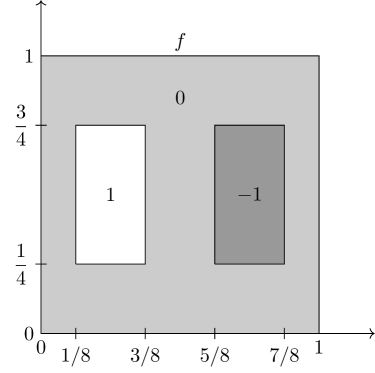
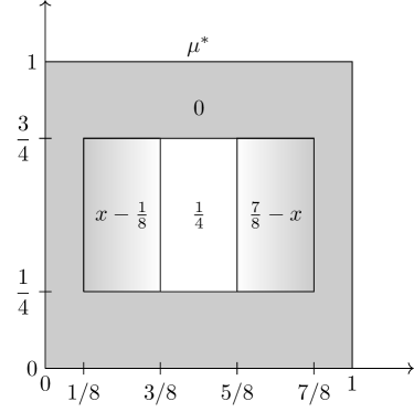
All our simulations address the test case proposed in [17] that considers a rigid transport of a unit density mass of rectangular shape from left to right. We look for the numerical solution of (1.2) defined on the domain and with forcing functions and (see Figure 1, left). The explicit solution for this problem is calculated in [10] and is given by:
| (7.3) |
and
| (7.4) |
The spatial distribution of is shown in Figure 1, right panel. This (apparently) simple test case captures most of the main challenges in solving the Monge-Kantorovich equations. In fact, the optimal transport density is zero in a large part of , leading to the degeneracy of the elliptic PDE in (1.2), and discontinuous across the segments that delimit the lower and upper boundary of its support, causing potential interpolation difficulties.
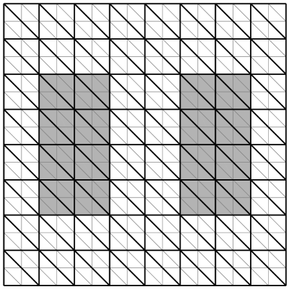
The space is defined by means of a sequence of meshes with . The coarsest mesh is a uniform triangulation of the unit square domain obtained by subdividing each side into intervals. Each subsequent mesh is obtained by uniform refinement of the previous one. Figure 2 shows the triangulations and used in the definition of and . The support of the forcing functions and , identified in the figure by gray areas, is aligned with the triangle edges to avoid any geometrical error. Automatically, the mesh results aligned with the entire support of .
7.2. Verification of Hypothesis 3.3
 |
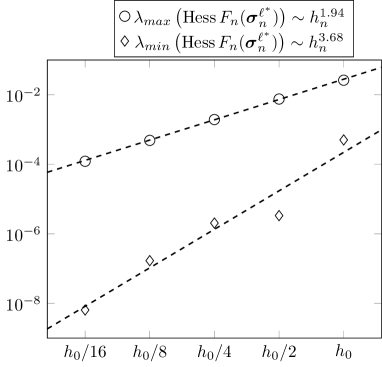 |
The numerical validation of Hypothesis 3.3 presents two difficulties. First, the conditions in (3.5) (3.6) are expressed in terms of a minimizer of , which is not known a priori. Second, the numerical evaluation of eq. (3.6) is not robust, because it requires some sort of threshold procedure to check In our experiments we consider the equivalent characterization of Hypothesis 3.3 given by Corollary 3.5 tested at the numerically computed optimum , i.e., we verify
Figure 3 shows the minimum () and maximum () for the mesh sequence for , where is denotes the mesh parameter of . We observe that the calculated minimum eigenvalues are always positive, suggesting that Hypothesis 3.3 is always verified at the numerical optimum. We note that the minimum eigenvalue tends to zero with at different rates depending on the chosen relaxation parameter . Namely, we observe experimentally that , in the case , and , in the case In addition, in both cases, the maximum and the minimum eigenvalues scale approximately at a constant rate, leading to an experimental spectral condition number of the Hessian that is proportional to in the case and to in the case .
7.3. Convergence of the gradient flow
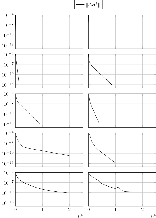
In Figure 4 we report the convergence profiles of Algorithm 2 when applied to the solution of our test case with constant time-step size on the different mesh levels ( top and bottom rows) and with (left and right columns). The -axis represents the quantity defined in (7.1), while the -axis represents time-steps (). The results shown in the first four rows correspond to mesh levels and clearly display the geometric convergence of the proposed method, as predicted by eq. (5.32) of Proposition 5.5. Indeed, after a short pre-asymtpotic phase, the curves are essentially straight lines. On the other hand, the last row, corresponding to , shows a slightly decreased experimental convergence rate with respect to our theoretical results, in particular in the last few time-steps. This saturation can be attributed to the errors in the numerical solution of the linear systems, which, from experimental calculations, are characterized by large condition numbers of the order . Indeed, increments smaller than would require a linear system solution with a residual norm smaller than , i.e., our machine precision.
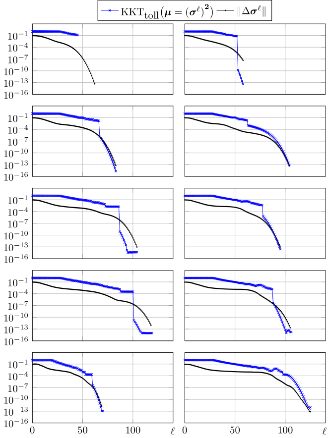
We repeat the same experiment using Algorithm 3 instead of Algorithm 2 and report the obtained results in Figure 5. Here the quantity is reported together with the approximate KKT condition residual defined in equation (7.2), which is used to experimentally verify that the computed critical point is indeed a minimum for the functional . The latter quantity naturally exhibits some drops due to the boolean nature of the test . In all the considered cases the super-exponential convergence predicted by eq.(6.3) and lines below is observed. This has a remarkable effect on the number of iterations needed to achieve a predefined precision, which, compared to the constant step case, drops by a multiplicative factor of approximately 100. Moreover, we observe that also the rate at which iterations grow as increases is slower when using Algorithm 3 instead of Algorithm 2. Finally, we note that the above mentioned saturation effect is weaker in these simulations with respect to the ones obtained by Algorithm 2.
7.4. Convergence towards
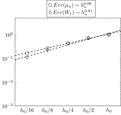

The last experiment is aimed at testing numerically the spatial convergence of the proposed method using the different mesh levels and the two choices of defined before. Figure 6 reports the related results in terms of the -norms of the errors on the minimizer, vs. , and the errors on the optimal transport energy, vs. . We would like to stress that the optimal value of the transport energy is precisely the Wasserstein-1 distance between and [17], i.e.:
The graph on the left is related to and shows that the convergence rate for both plotted quantities is smaller than 1, with a slightly greater convergence rate for the Wasserstein-1 (0.81 vs. 0.66). These results are a consequence of error saturation arising from the first order convergence of towards zero. On the other hand, the convergence profiles for the case of the right panel display superlinear convergence rates. The transport density converges towards the optimal value with a calculated rate of 1.38, while the Wasserstein-1 distance displays full second order convergence in accordance with the rate of convergence to zero of . We would like to note that similar results were found in [6], where the algorithm proposed in [17] was extended to address OT problems defined on three-dimensional embedded surfaces. The algorithm used in [17] differs from Algorithm 3 in the fact that forward Euler is used in place of backward Euler and , leading to obvious restrictions on time-step sizes and considerably higher computational costs. The obtained experimental results showed a third order convergence rate attributable to the absence of error saturation effects caused by the presence of .
Acknowledgments
References
- [1] L. Ambrosio, L. A. Caffarelli, Y. Brenier, G. Buttazzo, and C. Villani, Optimal transportation and applications, vol. 1813 of Lecture Notes in Mathematics, Springer-Verlag, Berlin; Centro Internazionale Matematico Estivo (C.I.M.E.), Florence, 2003. Lectures from the C.I.M.E. Summer School held in Martina Franca, September 2–8, 2001, Edited by Caffarelli and S. Salsa.
- [2] L. Ambrosio, N. Gigli, and G. Savaré, Gradient flows in metric spaces and in the space of probability measures, Lectures in Mathematics ETH Zürich, Birkhäuser Verlag, Basel, second ed., 2008.
- [3] J. Benamou, T. O. Gallouët, and F. Vialard, Second-order models for optimal transport and cubic splines on the wasserstein space, Found. Comput. Math., 19 (2019), p. 1113–1143.
- [4] J.-D. Benamou and G. Carlier, Augmented Lagrangian methods for transport optimization, mean field games and degenerate elliptic equations, J. Opt. Theory. Appl., 167 (2015), pp. 1–26.
- [5] R. J. Berman, Convergence rates for discretized monge–ampère equations and quantitative stability of optimal transport, Found. Comput. Math., 21 (2022), p. 1099–1140.
- [6] L. Berti, E. Facca, and M. Putti, Numerical solution of the L1-optimal transport problem on surfaces, Comp. Meth. Appl., submitted (2022).
- [7] D. P. Bertsekas, Nonlinear programming, Athena Scientific, 2nd ed., 1999.
- [8] J. Bolte, A. Daniilidis, and A. Lewis, The Łojasiewicz inequality for nonsmooth subanalytic functions with applications to subgradient dynamical systems, SIAM J. Optim., 17 (2006), pp. 1205–1223.
- [9] G. Bouchitté, G. Buttazzo, and P. Seppecher, Shape optimization solutions via Monge-Kantorovich equation, C. R. Acad. Sci. Paris Sér. I Math., 324 (1997), pp. 1185–1191.
- [10] G. Buttazzo and E. Stepanov, On regularity of transport density in the Monge–Kantorovich problem., SIAM J. Control Optim., 42 (2003), pp. 1044–1055.
- [11] J. Carrillo, K. Craig, L. Wang, and C. Wei, Primal dual methods for wasserstein gradient flows, Found. Comput. Math., 22 (2022), p. 389–443.
- [12] R. Chill, On the Łojasiewicz-Simon gradient inequality, J. Funct. Anal., 201 (2003), pp. 572–601.
- [13] M. Cuturi, Sinkhorn distances: Lightspeed computation of optimal transport, in Advances in neural information processing systems, 2013, pp. 2292–2300.
- [14] G. Dal Maso, An introduction to -convergence, vol. 8 of Progress in Nonlinear Differential Equations and their Applications, Birkhäuser Boston, Inc., Boston, MA, 1993.
- [15] L. C. Evans and W. Gangbo, Differential equations methods for the Monge-Kantorovich mass transfer problem, Mem. Amer. Math. Soc., 137 (1999), pp. viii+66.
- [16] E. Facca, F. Cardin, and M. Putti, Towards a stationary Monge-Kantorovich dynamics: the Physarum Polycephalum experience, SIAM J. Appl. Math., 78 (2018), pp. 651–676.
- [17] E. Facca, S. Daneri, F. Cardin, and M. Putti, Numerical solution of Monge-Kantorovich equations via a dynamic formulation, J. Sci. Comput., 82 (2020), pp. Paper No. 68, 26.
- [18] E. Facca, F. Piazzon, and M. Putti, Transport energy, Appl. Math. Opt., 86 (2022).
- [19] M. Feldman and R. J. McCann, Uniqueness and transport density in Monge’s mass transportation problem, Calc. Var. Partial Differ. Equ., 15 (2002), pp. 81–113.
- [20] O. Güler, On the convergence of the proximal point algorithm for convex minimization, SIAM J. Control Optim., 29 (1991), pp. 403–419.
- [21] A. Haraux and Jendoubi, Decay estimates to equilibrium for some evolution equations with an analytic nonlinearity, Asymptot. Anal., 26 (2001), pp. 21–36.
- [22] D. Hauer and J. M. Mazón, Kurdyka-Łojasiewicz-Simon inequality for gradient flows in metric spaces, Trans. Amer. Math. Soc., 372 (2019), pp. 4917–4976.
- [23] L. Kantorovitch, On the translocation of masses, C. R. (Doklady) Acad. Sci. URSS (N.S.), 37 (1942), pp. 199–201.
- [24] W. Li, E. K. Ryu, S. Osher, W. Yin, and W. Gangbo, A parallel method for earth mover’s distance, J. Scient. Comput., 75 (2018), pp. 182–197.
- [25] S. Łojasiewicz, Une propriété topologique des sous-ensembles analytiques réels, in Les Équations aux Dérivées Partielles (Paris, 1962), Éditions du Centre National de la Recherche Scientifique (CNRS), 1963, pp. 87–89.
- [26] B. Merlet and M. Pierre, Convergence to equilibrium for the backward Euler scheme and applications, Commun. Pure Appl. Anal., 9 (2010), pp. 685–702.
- [27] G. Monge, Mémoire sur la théorie des déblais et des remblais, Histoire de l’Académie Royale des Sciences de Paris, (1791), pp. 666–704.
- [28] G. Peyré and M. Cuturi, Computational optimal transport: With applications to data science, Found. Trends Mach. Learn., 11 (2019), pp. 355–607.
- [29] R. T. Rockafellar, Monotone operators and the proximal point algorithm, SIAM J. Control Optim., 14 (1976), pp. 877–898.
- [30] F. Santambrogio, Introduction to optimal transport theory, in Optimal transportation, vol. 413 of London Math. Soc. Lecture Note Ser., Cambridge Univ. Press, Cambridge, 2014, pp. 3–21.
- [31] , Optimal transport for applied mathematicians, vol. 87 of Progress in Nonlinear Differential Equations and their Applications, Birkhäuser/Springer, Cham, 2015. Calculus of variations, PDEs, and modeling.