Spherical Inducing Features for Orthogonally-Decoupled Gaussian Processes

Abstract

Despite their many desirable properties, Gaussian processes (gps) are often compared unfavorably to deep neural networks (nns) for lacking the ability to learn representations. Recent efforts to bridge the gap between gps and deep nns have yielded a new class of inter-domain variational gps in which the inducing variables correspond to hidden units of a feedforward nn. In this work, we examine some practical issues associated with this approach and propose an extension that leverages the orthogonal decomposition of gps to mitigate these limitations. In particular, we introduce spherical inter-domain features to construct more flexible data-dependent basis functions for both the principal and orthogonal components of the gp approximation and show that incorporating nn activation features under this framework not only alleviates these shortcomings but is more scalable than alternative strategies. Experiments on multiple benchmark datasets demonstrate the effectiveness of our approach.

1 Introduction

Gaussian processes (gps) provide a powerful framework for reasoning about unknown functions and are ubiquitous in probabilistic machine learning (Rasmussen & Williams, 2006). They are data-efficient, innately robust to over-fitting, and can flexibly encode priors through their covariance function. Last but not least, by virtue of their ability to faithfully capture predictive uncertainty, they form the backbone of many sequential decision-making methods that require reliable uncertainty estimates to balance trade-offs such as exploration and exploitation, e.g. in reinforcement learning (Deisenroth & Rasmussen, 2011), Bayesian optimization (Garnett, 2023), and probabilistic numerics (Hennig et al., 2022). In spite of their many advantages, gps are often compared unfavourably to deep neural networks (nns) for their poor scalability to large datasets, and their inability to capture rich hierarchies of abstract representations (Calandra et al., 2016; Wilson et al., 2016; Ober et al., 2021). While gps are the infinite-width limit of nns and therefore, in theory, have infinitely more basis functions (Neal, 1996), these basis functions are static and fully determined by the covariance function (MacKay et al., 1998). This makes it difficult for gps to flexibly adapt to complex and structured data from which it is beneficial for the basis functions to learn and encode useful representations.

Considerable research effort has been devoted to sparse approximations for gps (Csató & Opper, 2002; Seeger et al., 2003; Quinonero-Candela & Rasmussen, 2005; Snelson & Ghahramani, 2005). Not least of these is sparse variational gps (svgps) (Titsias, 2009; Hensman et al., 2013, 2015a). Such advances have not only improved the scalability of gps, but also unlocked more flexibility in model specification. In particular, the use of inter-domain inducing variables in svgp (Lázaro-Gredilla & Figueiras-Vidal, 2009) effectively equips the gp approximation with data-dependent basis functions. Recent works have exploited this to construct a new family of svgp models in which the basis functions correspond to activations of a feed-forward nn (Sun et al., 2020; Dutordoir et al., 2021). By stacking multiple layers to form a deep gp (dgp) (Damianou & Lawrence, 2013), the propagation of the predictive distribution accurately resembles a forward-pass through a deep nn.

In this paper, we show that while this approach results in a posterior predictive with a more expressive mean, the variance estimate is typically less accurate and tends to be over-dispersed. Additionally, we examine some practical challenges associated with this method, such as limitations on the use of certain popular kernel and nn activation choices. To address these issues, we propose an extension that aims to mitigate these limitations. Specifically, when viewed from the function-space perspective, the posterior predictive of svgp depends on a single set of basis functions that is determined by only a finite collection of inducing variables. Recent advances introduce an orthogonal set of basis functions as a means of capturing additional variations remaining from the standard basis (Salimbeni et al., 2018; Cheng & Boots, 2017; Shi et al., 2020). We extend this framework by introducing inter-domain variables to construct more flexible data-dependent basis functions for both the standard and orthogonal components. In particular, we show that incorporating nn activation inducing functions under this framework is an effective way to ameliorate the aforementioned shortcomings. Our experiments on numerous benchmark datasets demonstrate that this extension leads to improvements in predictive performance against comparable alternatives.

2 Background

Gaussian processes (gps) are a flexible class of distributions over functions. A random function $f:\mathcal{X}\to\mathbb{R}$ on some domain $\mathcal{X}\subseteq\mathbb{R}^{d}$ is distributed according to a gp if, at any finite collection of input locations $\mathbf{X}_{\ast}\subseteq\mathcal{X}$, its values $\mathbf{f}_{\ast}=f(\mathbf{X}_{\ast})$ follow a Gaussian distribution. A gp is fully determined by its mean function, which can be assumed without loss of generality to be constant (e.g. zero), and its covariance function $k(\mathbf{x},\mathbf{x}^{\prime})$.

Consider a supervised learning problem in which we have a dataset $\{\mathbf{x}_{n},y_{n}\}_{n=1}^{N}$ consisting of scalar outputs $y_{n}$, which are related to $f_{n}\triangleq f(\mathbf{x}_{n})$, the value of some unknown function $f(\cdot)$ at input $\mathbf{x}_{n}\in\mathcal{X}$, through the likelihood $p(y_{n}\,|\,f_{n},\theta)$. A powerful modelling approach consists of specifying a gp prior on the latent function $f(\cdot)$,

$$f(\mathbf{x})\sim\mathcal{GP}\left(0,k(\mathbf{x},\mathbf{x}^{\prime})\right).$$ (1)

Let $\mathbf{X}$ denote the inputs, $\mathbf{f}$ the corresponding latent function values, and $\mathbf{y}$ the outputs. In the regression setting, the outputs $\mathbf{y}$ are noisy observations of the latent values $\mathbf{f}$, typically related through a Gaussian likelihood $p(\mathbf{y}\,|\,\mathbf{f},\theta)=\mathcal{N}(\mathbf{y}\,|\,\mathbf{f},\beta^{-1}\mathbf{I})$ for some precision $\beta>0$. In this case, although the posterior $p(\mathbf{f}\,|\,\mathbf{y})$ is analytically tractable, its computation has time complexity $\mathcal{O}(N^{3})$.

2.1 Sparse Gaussian processes

A range of sparse gp methods have been developed over the years to mitigate these limitations (Csató & Opper, 2002; Seeger et al., 2003; Quinonero-Candela & Rasmussen, 2005; Snelson & Ghahramani, 2005). Broadly, in sparse gps, one summarizes $f(\cdot)$ succinctly in terms of inducing variables, which are values $\mathbf{u}\triangleq f(\mathbf{Z})$ taken at a collection of $M$ (usually $M\ll N$) locations $\mathbf{Z}=[\mathbf{z}_{1}\cdots\mathbf{z}_{M}]^{\top}$, where $\mathbf{z}_{m}\in\mathcal{X}$. Not least among these approaches is sparse variational gp (svgp), which casts sparse gps within the framework of variational inference (vi) (Titsias, 2009; Hensman et al., 2013, 2015a).

Specifically, the joint distribution of the model augmented by inducing variables $\mathbf{u}$ is $p(\mathbf{y},\mathbf{f},\mathbf{u})=p(\mathbf{y}\,|\,\mathbf{f})p(\mathbf{f},\mathbf{u})$ where $p(\mathbf{f},\mathbf{u})=p(\mathbf{f}\,|\,\mathbf{u})p(\mathbf{u})$ for prior $p(\mathbf{u})=\mathcal{N}(\mathbf{0},\mathbf{K}_{\mathbf{u}\mathbf{u}})$ and conditional

$$p(\mathbf{f}\,|\,\mathbf{u})=\mathcal{N}(\mathbf{f}\,|\,\mathbf{Q}_{\mathbf{f}\mathbf{u}}\mathbf{u},\mathbf{K}_{\mathbf{f}\mathbf{f}}-\mathbf{Q}_{\mathbf{f}\mathbf{f}}),$$ (2)

where $\mathbf{Q}_{\mathbf{f}\mathbf{f}}\triangleq\mathbf{Q}_{\mathbf{f}\mathbf{u}}\mathbf{K}_{\mathbf{u}\mathbf{u}}\mathbf{Q}_{\mathbf{u}\mathbf{f}}$ and $\mathbf{Q}_{\mathbf{f}\mathbf{u}}\triangleq\mathbf{K}_{\mathbf{f}\mathbf{u}}\mathbf{K}_{\mathbf{u}\mathbf{u}}^{-1}$. The joint variational distribution is defined as $q(\mathbf{f},\mathbf{u})\triangleq p(\mathbf{f}\,|\,\mathbf{u})q(\mathbf{u})$, where $q(\mathbf{u})\triangleq\mathcal{N}\left(\mathbf{m}_{\mathbf{u}},\mathbf{C}_{\mathbf{u}}\right)$ for variational parameters $\mathbf{m}_{\mathbf{u}}\in\mathbb{R}^{M}$ and $\mathbf{C}_{\mathbf{u}}\in\mathbb{R}^{M\times M}$ s.t. $\mathbf{C}_{\mathbf{u}}\succeq 0$. Integrating out $\mathbf{u}$ yields the posterior predictive

$$q(\mathbf{f}_{\ast})=\mathcal{N}\left(\mathbf{Q}_{\ast\mathbf{u}}\mathbf{m}_{\mathbf{u}},\mathbf{K}_{\ast\ast}-\mathbf{Q}_{\ast\mathbf{u}}(\mathbf{K}_{\mathbf{u}\mathbf{u}}-\mathbf{C}_{\mathbf{u}})\mathbf{Q}_{\mathbf{u}\ast}\right),$$

where parameters $\mathbf{m}_{\mathbf{u}}$ and $\mathbf{C}_{\mathbf{u}}$ are learned by minimizing the Kullback–Leibler (kl) divergence between the approximate and exact posterior, $\textsc{kl}\left[q(\mathbf{f})\;\|\;p(\mathbf{f}\,|\,\mathbf{y})\right]$. Thus seen, svgp has time complexity $\mathcal{O}(M^{3})$ at prediction time and $\mathcal{O}(M^{3}+M^{2}N)$ during training.

In the reproducing kernel Hilbert space (rkhs) associated with $k$, the predictive has a dual representation in which the mean and covariance share the same basis determined by $\mathbf{u}$ (Cheng & Boots, 2017; Salimbeni et al., 2018). More specifically, the basis function is effectively the vector-valued function $\mathbf{k}_{\mathbf{u}}:\mathcal{X}\to\mathbb{R}^{M}$ whose $m$-th component is defined as

$$\left[\mathbf{k}_{\mathbf{u}}(\mathbf{x})\right]_{m}\triangleq\mathrm{Cov}\left(f(\mathbf{x}),u_{m}\right).$$ (3)

In the standard definition of inducing points, $\left[\mathbf{k}_{\mathbf{u}}(\mathbf{x})\right]_{m}=k(\mathbf{z}_{m},\mathbf{x})$, so the basis function is solely determined by $k$ and the local influence of pseudo-input $\mathbf{z}_{m}$.

Inter-domain inducing features are a generalization of standard inducing variables in which each variable $u_{m}\triangleq L_{m}[f]$ for some linear operator $L_{m}:\mathbb{R}^{\mathcal{X}}\to\mathbb{R}$. A particularly useful operator is the integral transform, $L_{m}[f]\triangleq\int_{\mathcal{X}}f(\mathbf{x})\phi_{m}(\mathbf{x})\,\mathrm{d}\mathbf{x}$, which was originally employed by Lázaro-Gredilla & Figueiras-Vidal (2009). Refer to the manuscript of van der Wilk et al. (2020) for a more thorough and contemporary treatment. A closely related form is the scalar projection of $f$ onto some $\phi_{m}$ in the rkhs $\mathcal{H}$,

$$L_{m}[f]\triangleq\langle f,\phi_{m}\rangle_{\mathcal{H}},$$ (4)

which leads to $\left[\mathbf{k}_{\mathbf{u}}(\mathbf{x})\right]_{m}=\phi_{m}(\mathbf{x})$ by the reproducing property of the rkhs. This, in effect, equips the gp approximation with basis functions $\phi_{m}$ that are not solely determined by the kernel, and suitable choices can lead to sparser representations and considerable computational benefits (Hensman et al., 2018; Burt et al., 2020; Dutordoir et al., 2020; Sun et al., 2021).

2.2 Spherical Harmonics Inducing Features

An instance of inter-domain features in the form of Equation 4 are the variational Fourier features (vffs) (Hensman et al., 2018), in which $\phi_{m}$ form an orthogonal basis of trigonometric functions. This formulation offers significant computational advantages but scales poorly beyond a small handful of dimensions. To address this, Dutordoir et al. (2020) propose a generalization of vffs using the spherical harmonics for $\phi_{m}$, which can be viewed as a multi-dimensional extension of the Fourier basis.

The construction relies on the Mercer decomposition of zonal kernels, which can be seen as the analog of stationary kernels in Euclidean spaces, but for hyperspheres. They can be expressed as $k(\mathbf{x},\mathbf{x}^{\prime})=\kappa\left(\tilde{\mathbf{x}}^{\top}\tilde{\mathbf{x}}^{\prime}\right)$ for some shape function $\kappa:[-1,1]\to\mathbb{R}$, where $\tilde{\boldsymbol{\eta}}\triangleq\frac{\boldsymbol{\eta}}{\lVert\boldsymbol{\eta}\rVert}\in\mathbb{S}^{d-1}$ for any $\boldsymbol{\eta}\in\mathbb{R}^{d}$ . Loosely speaking, just as stationary kernels are determined by the distance between inputs, zonal kernels depend only on the angle between inputs.

The spherical harmonics form an orthonormal basis on $L_{2}(\mathbb{S}^{d-1})$ consisting of the eigenfunctions of the kernel operator $\mathcal{K}$: $\mathcal{K}{Y}_{\ell,j}=a_{\ell}{Y}_{\ell,j}$, where ${Y}_{\ell,j}$ is the spherical harmonic of level $\ell$ and order $j$, and $a_{\ell}$ is the corresponding eigenvalue, or Fourier coefficient. Conveniently, by the Funk-Hecke theorem, $a_{\ell}$ can be computed by the one-dimensional integral

$$a_{\ell}=\frac{\Omega_{d}}{C_{\ell}^{(\alpha)}(1)}\int_{-1}^{1}\kappa(t)C_{\ell}^{(\alpha)}(t)(1-t^{2})^{\frac{d-3}{2}}\,\mathrm{d}t,$$

where $C_{\ell}^{(\alpha)}$ is the Gegenbauer polynomial of degree $\ell$ and $\alpha\triangleq\frac{(d-1)}{2}$. Now, the number $J({d},{\ell})$ of spherical harmonics that exist at a given level $\ell$ is determined by the multiplicity of eigenvalue $a_{\ell}$. Thus, $\kappa(t)$ can be represented by

$$\kappa(t)=\lVert\boldsymbol{\xi}\rVert\lVert\boldsymbol{\xi}^{\prime}\rVert\sum_{\ell=0}^{\infty}\sum_{j=1}^{J({d},{\ell})}a_{\ell}{Y}_{\ell,j}(\tilde{\boldsymbol{\xi}}){Y}_{\ell,j}(\tilde{\boldsymbol{\xi}}^{\prime}),$$ (5)

where $t\triangleq\tilde{\boldsymbol{\xi}}^{\top}\tilde{\boldsymbol{\xi}}^{\prime}$ for $\boldsymbol{\xi},\boldsymbol{\xi}^{\prime}\in\mathbb{R}^{d}$. Refer to the manuscript (Appendix B) of Dutordoir et al. (2021) for a concise summary of spherical harmonics in multiple dimensions.

Importantly, Equation 5 directly yields a Mercer decomposition for zonal kernels. In particular, let $\lambda_{\ell}$ denote the Fourier coefficients associated with kernel $k$. This gives rise to the inter-domain features $\phi_{m}\triangleq{Y}_{\ell,j}$, where $m$ indexes the pairs $(\ell,j)$. Crucially, this leads to a diagonal covariance

$$\left[\mathbf{K}_{\mathbf{u}\mathbf{u}}\right]_{mm^{\prime}}\triangleq\mathrm{Cov}\left(u_{m},u_{m^{\prime}}\right)=\lambda_{m}^{-1}\delta_{mm^{\prime}},$$

where $\lambda_{m}\triangleq\lambda_{\ell}$ and $\delta$ denotes the Kronecker delta.

2.3 Neural Network Inducing Features

The recent works of Sun et al. (2020); Dutordoir et al. (2021) aim to construct inter-domain features $\phi_{m}$ such that $\mathbf{k}_{\mathbf{u}}(\mathbf{x})$ in Equation 3 corresponds to a hidden layer in a feed-forward nn: $\sigma(\boldsymbol{\beta}\mathbf{x})$, for some $\boldsymbol{\beta}\in\mathbb{R}^{M\times d}$ and activation $\sigma$ such as the softplus or the rectified linear unit (relu) function.

In particular, let $H_{m}:\mathcal{X}\to\mathbb{R}$ denote the output of the $m$-th hidden unit. Additionally, let us project this function onto the unit hypersphere,

$$H_{m}(\mathbf{x})\triangleq\lVert\mathbf{z}_{m}\rVert\lVert\mathbf{x}\rVert\cdot\sigma\left(\frac{\mathbf{z}_{m}^{\top}\mathbf{x}}{\lVert\mathbf{z}_{m}\rVert\lVert\mathbf{x}\rVert}\right).$$ (6)

Now, since this function is itself zonal, it can be represented in terms of the spherical harmonics as in Equation 5. Let $\varsigma_{\ell}$ denote its associated Fourier coefficient. Thus, the inter-domain features can be defined as $\phi_{m}\triangleq H_{m}$, which leads to the covariance

$$\left[\mathbf{K}_{\mathbf{u}\mathbf{u}}\right]_{mm^{\prime}}=\sum_{\begin{subarray}{c}\ell=0:\\ \lambda_{\ell}\neq 0\end{subarray}}^{\infty}\frac{\varsigma_{\ell}^{2}}{\lambda_{\ell}}\frac{\ell+\alpha}{\alpha}C_{\ell}^{(\alpha)}\left(\frac{\mathbf{z}_{m}^{\top}\mathbf{z}_{m^{\prime}}}{\lVert\mathbf{z}_{m}\rVert\lVert\mathbf{z}_{m^{\prime}}\rVert}\right),$$ (7)

where $\lambda_{\ell}$ denotes the Fourier coefficients associated with kernel $k$. This formulation, which we refer to as activated svgp, has been shown to produce competitive results, especially when multiple activated svgp layers are stacked to form a dgp (Damianou & Lawrence, 2013), such that the propagation of the predictive means closely emulates a forward-pass through a deep nn.

Despite these favorable properties, activated svgps have several limitations when it comes to their use with common covariance functions. Before elaborating on them in § 3, we discuss the orthogonally-decoupled gp framework on which our proposed extension relies.

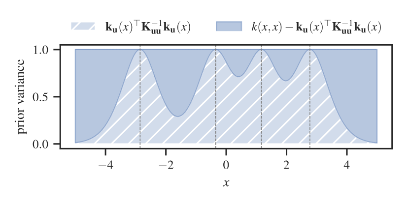
Figure 1: Prior variance deconstructed. The prior variance of $f(\mathbf{x})$ is $k(\mathbf{x},\mathbf{x})=\alpha$ for kernel amplitude $\alpha=1$, which can be decomposed as the sum of the prior variances of $g(\mathbf{x})$ and $h(\mathbf{x})$. Vertical dashed lines indicate the location of inducing inputs $\mathbf{z}_{m}$ for $m=1,\dotsc,4$. At these locations, the variance of $g(\mathbf{x})$ is 1 while that of $h(\mathbf{x})$ is 0.

2.4 Orthogonally Decoupled Inducing Points

Recent work has improved the efficiency of sparse gp methods through the structured decoupling of inducing variables (Cheng & Boots, 2017; Salimbeni et al., 2018; Shi et al., 2020). This not only enables the use of more variables at a reduced computational expense but also allows for more flexibility in modelling the predictive mean and covariance independently. We focus on the general framework of Shi et al. (2020) under which its predecessors can be subsumed.

Table 1: Summary of notation: relationships between input locations and output variables.

	$\mathbf{W}$	$\mathbf{X}$	$\mathbf{Z}$
$f(\cdot)$	$\mathbf{v}$	$\mathbf{f}$	$\mathbf{u}$
$h(\cdot)$	$\mathbf{v}^{\prime}$	$\mathbf{h}$	-

In particular, let the random function $f(\mathbf{x})$ from Equation 1 be decomposed into the sum of two independent gps: $f(\mathbf{x})=g(\mathbf{x})+h(\mathbf{x})$, where

$$g(\mathbf{x})\sim\mathcal{GP}(0,\mathbf{k}_{\mathbf{u}}^{\top}(\mathbf{x})\mathbf{K}_{\mathbf{u}\mathbf{u}}^{-1}\mathbf{k}_{\mathbf{u}}(\mathbf{x}^{\prime})),h(\mathbf{x})\sim\mathcal{GP}(0,s(\mathbf{x},\mathbf{x}^{\prime}))$$

and let the covariance function $s(\mathbf{x},\mathbf{x}^{\prime})$ be defined according to the Schur complement of $\mathbf{K}_{\mathbf{u}\mathbf{u}}$,

$$s(\mathbf{x},\mathbf{x}^{\prime})\triangleq k(\mathbf{x},\mathbf{x}^{\prime})-\mathbf{k}_{\mathbf{u}}^{\top}(\mathbf{x})\mathbf{K}_{\mathbf{u}\mathbf{u}}^{-1}\mathbf{k}_{\mathbf{u}}(\mathbf{x}^{\prime}),$$

where $\mathbf{k}_{\mathbf{u}}$ is defined in Equation 3. Intuitively, one can view $g$ as the projection of $f$ onto $\mathbf{u}$, and $h\perp g$, i.e. $h$ is orthogonal to $g$ (Hensman et al., 2018) in the statistical sense of linear independence (Rodgers et al., 1984). See Figure 1 for an illustration of the priors of $g(\mathbf{x})$ and $h(\mathbf{x})$. Let $\mathbf{h}$ be the values of $h$ at observed inputs $\mathbf{X}$, i.e. $\mathbf{h}\triangleq h(\mathbf{X})$. Then we have $p(\mathbf{h})=\mathcal{N}(\mathbf{0},\mathbf{S}_{\mathbf{f}\mathbf{f}})$, where $\mathbf{S}_{\mathbf{f}\mathbf{f}}\triangleq\mathbf{K}_{\mathbf{f}\mathbf{f}}-\mathbf{Q}_{\mathbf{f}\mathbf{f}}$. This allows one to reparameterize $\mathbf{f}\sim p(\mathbf{f}\,|\,\mathbf{u})$ from Equation 2, for a given $\mathbf{u}$, as

$$\mathbf{f}=\mathbf{Q}_{\mathbf{f}\mathbf{u}}\mathbf{u}+\mathbf{h},\qquad\mathbf{h}\sim p(\mathbf{h}).$$ (8)

The model’s joint distribution can now be written as $p(\mathbf{y},\mathbf{h},\mathbf{u})=p(\mathbf{y}\,|\,\mathbf{h},\mathbf{u})p(\mathbf{h})p(\mathbf{u})$, where $p(\mathbf{y}\,|\,\mathbf{h},\mathbf{u})=\mathcal{N}(\mathbf{y}\,|\,\mathbf{Q}_{\mathbf{f}\mathbf{u}}\mathbf{u}+\mathbf{h},\beta^{-1}\mathbf{I})$. Next, orthogonal inducing variables $\mathbf{v}$, which represent the values of $f$ at a collection of $K$ orthogonal inducing locations $\mathbf{W}\triangleq[\mathbf{w}_{1}\cdots\mathbf{w}_{K}]^{\top}$, are introduced. Similarly, inducing variables $\mathbf{v}^{\prime}$ represent the values of $h$ at $\mathbf{W}$. The reader may find it helpful to refer to Table 1 for a summary of the relationships between the input locations and the output variables defined thus far.

Now, by definition, $\mathbf{v}=\mathbf{Q}_{\mathbf{v}\mathbf{u}}\mathbf{u}+\mathbf{v}^{\prime}$, where $\mathbf{Q}_{\mathbf{v}\mathbf{u}}\triangleq\mathbf{K}_{\mathbf{v}\mathbf{u}}\mathbf{K}_{\mathbf{u}\mathbf{u}}^{-1}$ which is analogous to the relationship between $\mathbf{f}$ and $\mathbf{h}$ in Equation 8. Therefore, one need only be concerned with the treatment of $\mathbf{v}^{\prime}$. The joint distribution of the model augmented by the variables $\mathbf{v}^{\prime}$ now becomes $p(\mathbf{y},\mathbf{h},\mathbf{u},\mathbf{v}^{\prime})=p(\mathbf{y}\,|\,\mathbf{h},\mathbf{u})p(\mathbf{u})p(\mathbf{h},\mathbf{v}^{\prime})$, where $p(\mathbf{h},\mathbf{v}^{\prime})=p(\mathbf{h}\,|\,\mathbf{v}^{\prime})p(\mathbf{v}^{\prime})$ for $p(\mathbf{v}^{\prime})=\mathcal{N}(\mathbf{0},\mathbf{S}_{\mathbf{v}\mathbf{v}})$ and $p(\mathbf{h}\,|\,\mathbf{v}^{\prime})=\mathcal{N}(\mathbf{h}\,|\,\mathbf{S}_{\mathbf{f}\mathbf{v}}\mathbf{S}_{\mathbf{v}\mathbf{v}}^{-1}\mathbf{v}^{\prime},\mathbf{S}_{\mathbf{f}\mathbf{f}}-\mathbf{S}_{\mathbf{f}\mathbf{v}}\mathbf{S}_{\mathbf{v}\mathbf{v}}^{-1}\mathbf{S}_{\mathbf{v}\mathbf{f}})$, with

$$\mathbf{S}_{\mathbf{v}\mathbf{f}}\triangleq\mathbf{K}_{\mathbf{v}\mathbf{f}}-\mathbf{Q}_{\mathbf{v}\mathbf{f}},\quad\mathbf{Q}_{\mathbf{v}\mathbf{f}}\triangleq\mathbf{Q}_{\mathbf{v}\mathbf{u}}\mathbf{K}_{\mathbf{u}\mathbf{u}}\mathbf{Q}_{\mathbf{u}\mathbf{f}},$$ (9)

$$\mathbf{S}_{\mathbf{v}\mathbf{v}}\triangleq\mathbf{K}_{\mathbf{v}\mathbf{v}}-\mathbf{Q}_{\mathbf{v}\mathbf{v}},\quad\mathbf{Q}_{\mathbf{v}\mathbf{v}}\triangleq\mathbf{Q}_{\mathbf{v}\mathbf{u}}\mathbf{K}_{\mathbf{u}\mathbf{u}}\mathbf{Q}_{\mathbf{u}\mathbf{v}}.$$ (10)

Let the variational distribution now be $q(\mathbf{h},\mathbf{u},\mathbf{v}^{\prime})=p(\mathbf{h}\,|\,\mathbf{v}^{\prime})q(\mathbf{u},\mathbf{v}^{\prime})$, where $q(\mathbf{u},\mathbf{v}^{\prime})\triangleq q(\mathbf{u})q(\mathbf{v}^{\prime})$ and $q(\mathbf{v}^{\prime})\triangleq\mathcal{N}\left(\mathbf{m}_{\mathbf{v}},\mathbf{C}_{\mathbf{v}}\right)$ for variational parameters $\mathbf{m}_{\mathbf{v}}\in\mathbb{R}^{K}$ and $\mathbf{C}_{\mathbf{v}}\in\mathbb{R}^{K\times K}$ s.t. $\mathbf{C}_{\mathbf{v}}\succeq 0$. This gives the posterior predictive density $q(\mathbf{f}_{\ast})=\mathcal{N}(\boldsymbol{\mu}_{\ast},\boldsymbol{\Sigma}_{\ast\ast})$, where

$$\boldsymbol{\mu}_{\ast} \triangleq\mathbf{Q}_{\ast\mathbf{u}}\mathbf{m}_{\mathbf{u}}+\mathbf{S}_{\ast\mathbf{v}}\mathbf{S}_{\mathbf{v}\mathbf{v}}^{-1}\mathbf{m}_{\mathbf{v}},$$ (11)

$$\begin{split}\boldsymbol{\Sigma}_{\ast\ast}&\triangleq\mathbf{K}_{\ast\ast}+\mathbf{Q}_{\ast\mathbf{u}}(\mathbf{C}_{\mathbf{u}}-\mathbf{K}_{\mathbf{u}\mathbf{u}})\mathbf{Q}_{\mathbf{u}\ast}\\ &\qquad+\mathbf{S}_{\ast\mathbf{v}}\mathbf{S}_{\mathbf{v}\mathbf{v}}^{-1}(\mathbf{C}_{\mathbf{v}}-\mathbf{S}_{\mathbf{v}\mathbf{v}})\mathbf{S}_{\mathbf{v}\mathbf{v}}^{-1}\mathbf{S}_{\mathbf{v}\ast}.\end{split}$$ (12)

Thus seen, prediction incurs a cost of $\mathcal{O}(M^{3}+K^{3})$ in this framework. Like the so-called odvgp framework of Salimbeni et al. (2018), when seen from the dual rkhs perspective, the predictive mean can be decomposed into a component that shares the same standard basis as the covariance, in addition to another component that is orthogonal to the standard basis. However, this framework extends odvgp further by also decomposing the predictive covariance into parts corresponding to the standard and orthogonal bases. Accordingly, setting $\mathbf{C}_{\mathbf{v}}=\mathbf{S}_{\mathbf{v}\mathbf{v}}$ recovers the odvgp framework, and further setting $\mathbf{m}_{\mathbf{v}}=\mathbf{0}$ recovers the standard svgp framework.

3 Methodology

We begin this section by outlining some of the limitations of activated svgps that preclude the use of numerous kernels and inducing features, not the least of which being popular choices of kernels such as the squared exponential (se) kernel and the Matérn family of kernels, combined with nn inducing features with relu activations.

The root cause of these issues can be seen in Figure 2, where the Fourier coefficients of various combinations of kernels and activation features are visualized. Specifically, for each combination, we compare the (root of the) kernel coefficients $\sqrt{\lambda_{\ell}}$ against the feature coefficients $\varsigma_{\ell}$ at increasing levels $\ell=1,\dotsc,35$. The posterior predictives that result from fitting activated svgp models with these combinations are shown in Figure 3. We consider the Matérn-$\nicefrac{{5}}{{2}}$ kernel as our running example, but the analysis extends to all stationary kernels.

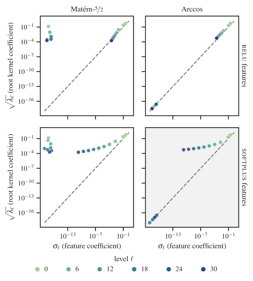
Figure 2: Comparison of the Fourier coefficients of various kernels and activation features for increasing levels $\ell=1,\dotsc,35$.

Spectra mismatch. For the Matérn kernel (left column of panes in Figures 2 and 3), we see that there are multiple levels $\ell$ at which the feature coefficients are zero while the corresponding kernel coefficients are nonzero. Such discrepancies in the spectra yields a poor Nyström approximation $\mathbf{Q}_{\mathbf{f}\mathbf{f}}$ that fails to fully capture the prior covariance $\mathbf{K}_{\mathbf{f}\mathbf{f}}$ induced by the kernel, which subsequently leads to the overestimation of the predictive variance and therefore a suboptimal evidence lower bound (elbo). In contrast, the Arccos kernel does not suffer from this pathology.

RKHS inner product. The rkhs inner product associated with zonal kernels in general is a series consisting of ratios of Fourier coefficients. Since the relu feature coefficients (top row of panes in Figures 2 and 3) decay at the same rate as the square root of the kernel coefficients, this results in a divergent series which in turn renders the rkhs inner product indeterminate. In contrast, the feature coefficients of the comparatively smoother softplus activation (bottom row of panes in Figures 2 and 3) decay at a much faster rate, and thus yields a well-defined rkhs inner product. For the reasons outlined above, the work of Dutordoir et al. (2021) restricted its scope to the use of the Arccos kernel in conjunction with the softplus activation (pane highlighted in gray in Figure 2).

Truncation error. Lastly, as expected, the truncation of the series in Equation 7 at some finite number $L$ of spherical harmonic levels often leads to overly smooth predictive response surfaces and overestimation of the variance.

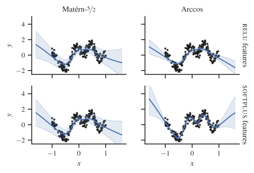
Figure 3: Posterior predictives of activated svgp models various kernels and activation features and $L=16$ levels.

Spherical Features for Orthogonally-Decoupled GPs

We propose extending the orthogonally-decoupled gp framework (§ 2.4) to use inter-domain inducing features. Accordingly, let $u_{m}\triangleq\langle f,\phi_{m}\rangle_{\mathcal{H}}$ and $v_{k}\triangleq\langle f,\psi_{k}\rangle_{\mathcal{H}}$ for some arbitrary choices of $\phi_{m},\psi_{k}\in\mathcal{H}$. This generalizes the framework of Shi et al. (2020) since, by the reproducing property, setting $\phi_{m}:\mathbf{x}\mapsto k(\mathbf{z}_{m},\mathbf{x})$ and $\psi_{k}:\mathbf{x}\mapsto k(\mathbf{w}_{k},\mathbf{x})$ leads to standard inducing points, $u_{m}=f(\mathbf{z}_{m}),v_{k}=f(\mathbf{w}_{k})$.

In particular, we define $\phi_{m}\triangleq H_{m}$, the $m$-th unit of the spherical activation layer (Equation 6) described in § 2.3, and $\psi_{k}(\mathbf{x})\triangleq k(\mathbf{w}_{k},\mathbf{x})$. The posterior predictive of the model described in § 2.4, summarized by Equations 11 and 12, is fully determined by the covariances $\mathbf{K}_{\mathbf{f}\mathbf{f}},\mathbf{K}_{\mathbf{u}\mathbf{f}},\mathbf{K}_{\mathbf{v}\mathbf{f}},\mathbf{K}_{\mathbf{u}\mathbf{u}},\mathbf{K}_{\mathbf{v}\mathbf{u}}$ and $\mathbf{K}_{\mathbf{v}\mathbf{v}}$. Recall that $\left[\mathbf{K}_{\mathbf{u}\mathbf{f}}\right]_{mn}=\left[\mathbf{k}_{\mathbf{u}}(\mathbf{x}_{n})\right]_{m}$ and $\mathbf{K}_{\mathbf{u}\mathbf{u}}$ is precisely as expressed in Equation 7. We have

$$\left[\mathbf{K}_{\mathbf{v}\mathbf{f}}\right]_{kn} \triangleq\mathrm{Cov}\left(v_{k},f(\mathbf{x}_{n})\right)=k(\mathbf{w}_{k},\mathbf{x}_{n}),$$

$$\left[\mathbf{K}_{\mathbf{v}\mathbf{u}}\right]_{km} \triangleq\mathrm{Cov}\left(v_{k},u_{m}\right)=\phi_{m}(\mathbf{w}_{k}),$$

$$\left[\mathbf{K}_{\mathbf{v}\mathbf{v}}\right]_{kk^{\prime}} \triangleq\mathrm{Cov}\left(v_{k},v_{k^{\prime}}\right)=k(\mathbf{w}_{k},\mathbf{w}_{k^{\prime}}).$$

Note that the cross-covariance $\mathbf{K}_{\mathbf{v}\mathbf{u}}$ between $\mathbf{u}$ and $\mathbf{v}$ can be interpreted as the forward-pass of the orthogonal pseudo-input $\mathbf{w}_{k}$ through the nn activation $H_{m}$. Crucially, these terms constitute the orthogonal basis and provide additional degrees of flexibility, through free parameters $\mathbf{W}$, that can compensate for errors remaining from the original basis—in both the predictive mean and variance. Suffice it to say, this is not the only possible choice but is one that possesses a number of appealing properties. We compare against a few other possibilities which we enumerate in Appendix A.

As discussed in § 2.4, the addition of $K$ inducing variables incurs a cost of $\mathcal{O}(M^{3}+K^{3})$. More precisely: suppose the exact cost is $C\cdot(M^{3}+K^{3})$ operations for some constant $C$ w.r.t. $M,K$. Further, suppose $K=B\cdot M$ for some $B>0$. Then there are a total of $(B+1)\cdot M$ inducing variables (orthogonal or otherwise) and the cost becomes $(B^{3}+1)C\cdot M^{3}$. By comparison, incorporating the same number of inducing variables in svgp costs $(B+1)^{3}C\cdot M^{3}$. That is, this approach leads to a $(B^{3}+1)$-fold increase in the constant rather than a $(B+1)^{3}$-fold increase. Concretely, this means that doubling the number of inducing variables doubles the constant in this approach, but leads to an eight-fold increase in svgp. While such a difference vanishes asymptotically for large $M$ and $K$, it still has a considerable impact for modest sizes ($M,K<1,000$) that are feasible in practice. Thus seen, incorporating an orthogonal basis spanned by $K$ inducing variables is a more cost-effective strategy for improving activated svgp than increasing $M$ or the truncation level $L$.

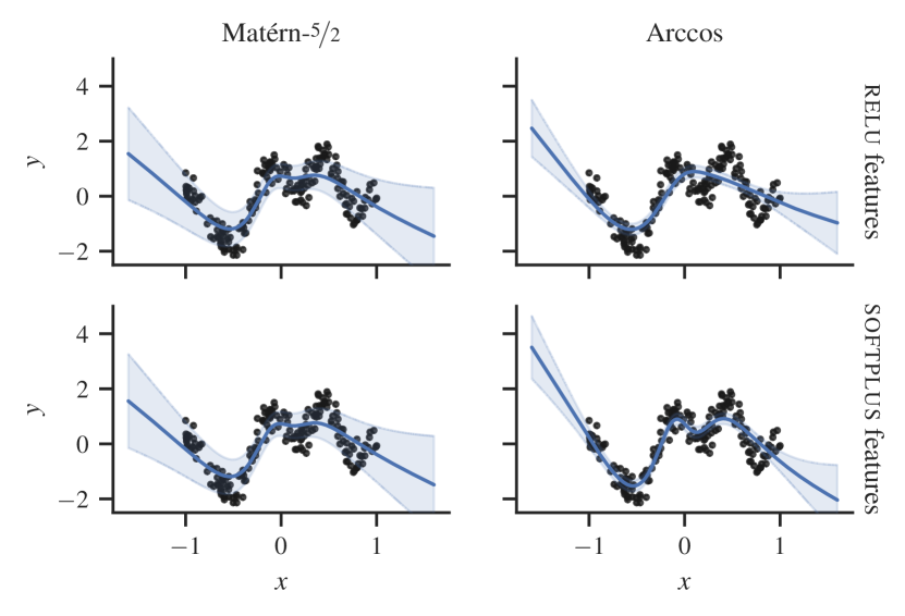
(a) Inducing activation features with $L=8$ levels.

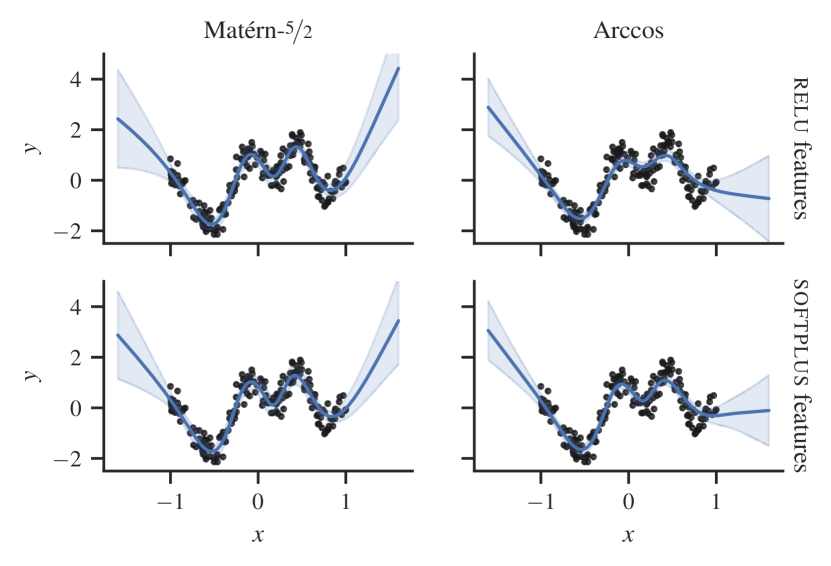
(b) Inducing activation features with $L=8$ levels and $K=8$ orthogonal bases (our method).

Figure 4: Posterior predictives of activated svgp with various kernels and activation features on the 1D Snelson dataset; black circular markers represent the observations; blue solid lines and shaded regions denote the mean and the $\pm 2$ standard deviations, resp.

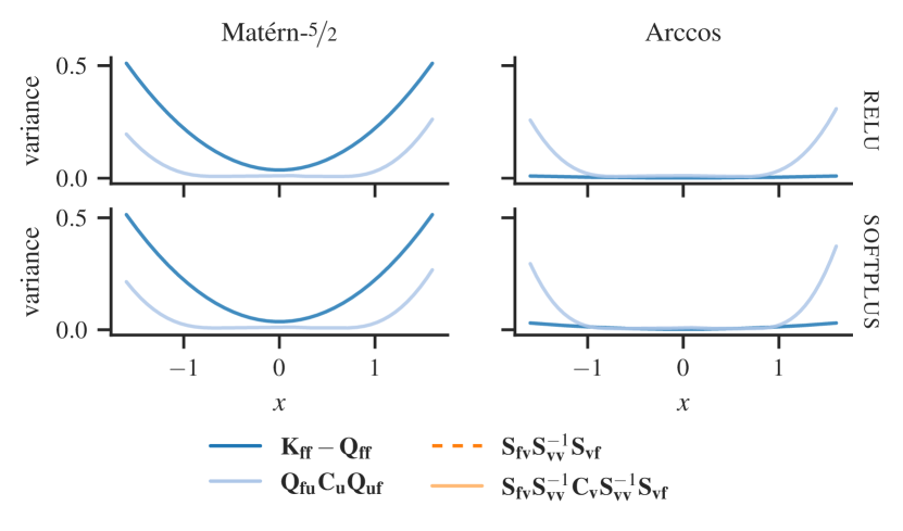
(a) Inducing activation features with $L=8$ levels.

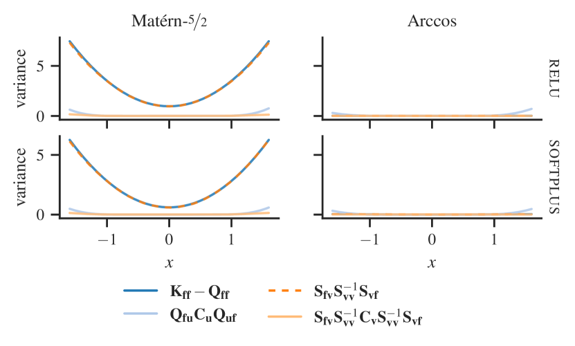
(b) Inducing activation features with $L=8$ levels and $K=8$ orthogonal bases (our method).

Figure 5: Decomposition of the posterior predictive variances of svgp with various kernels and activation features on the 1D snelson dataset (see Figure 4) into its constituent terms; the additive terms that constitute the predictive variance are indicated by solid lines, while the subtractive terms are indicated by dashed lines; terms that constitute the predictive variance of the original svgp model (Titsias, 2009) have a blue hue, while additional terms introduced by the orthogonally-decoupled model (Shi et al., 2020) have an orange hue.

4 Experiments

We describe the experiments conducted to empirically validate our approach. The open-source implementation of our method can be found at: ltiao/spherical-orthogonal-gaussian-processes. Further information concerning the experimental set-up and various implementation details can be found in Appendix B.

4.1 Synthetic 1D Dataset

We highlight some notable properties of our method on the one-dimensional dataset of Snelson & Ghahramani (2007).

First we fit activated svgp models with different combinations of kernels and activation features using $L=8$ truncation levels. The resulting posterior predictives are shown in Figure 4. More specifically, in Figure 4(a), we see that none of the model fits are particularly tight due in part to truncation errors, since we are using relatively few levels. This is especially true of the Matérn kernel (left column of panes), which results in a posterior that is not only too smooth but also clearly suffering from an overestimation of the variance. A conceptually straightforward way to improve performance is to increase the truncation level. Accordingly, Figure 3 (introduced earlier in § 3) showed results from effectively the exact same set-up, but with twice the number of levels ($L=16$). With this increase, we see a clear improvement in the Arccos-softplus case, but no discernible difference in the other combinations. Notably, the overestimation of the variances in the Matérn kernel persists. By comparison, Figure 4(b) shows results from using $L=8$ truncation levels, but with the addition of $K=8$ orthogonal inducing variables. Remarkably, incorporating just a handful of these variables produces substantial improvements, not least for the Matérn kernel.

Figure 5 offers a deeper insight into the underlying mechanisms that contribute to these improvements. Here we plot the predictive variance (Equation 12) in terms of its constituent parts. In Figure 5(a), we see that the variance estimate with Matérn kernels is heavily distorted by large spurious contributions in the $\mathbf{K}_{\mathbf{f}\mathbf{f}}-\mathbf{Q}_{\mathbf{f}\mathbf{f}}$ term (dark blue solid line), which is caused by the pathology described in § 3. On the other hand, in Figure 5(b), such spurious contributions also appear, but are offset by the subtractive term $\mathbf{S}_{\mathbf{f}\mathbf{v}}\mathbf{S}_{\mathbf{v}\mathbf{v}}^{-1}\mathbf{S}_{\mathbf{v}\mathbf{f}}$ (dark orange dashed line). This term constitutes the orthogonal basis, and provides added flexibility that is effective at nullifying errors introduced by the original basis.

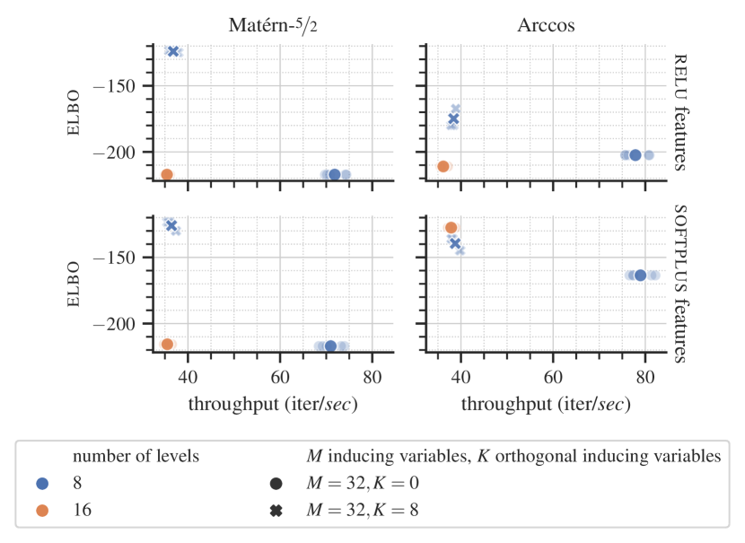
Figure 6: The elbo and throughput (of model fitting) for various kernels and activation features and the configurations visualized in Figure 3, Figures 4(a) and 5(a), and Figures 4(b) and 5(b); markers with low opacity represent the individual runs, while markers with high opacity represent the mean of each group.

Each of the three variations discussed above are repeated 5 times, and some quantitative results are summarized in Figure 6. Specifically, we report the elbo and the throughput, i.e. the average number of optimization iterations completed per second. The activated svgp with $L=8$ truncation levels, as seen in Figures 4(a) and 5(a), is represented by the blue circular markers. The model resulting from doubling the number of levels $L=16$, as seen in Figure 3, is represented by the orange circular markers. As discussed, this leads to an improvement in the Arccos-softplus case, but to modest or no improvements otherwise. However, we can now see that this has come at a significant computational expense, as the throughput has reduced by roughly half. On the other hand, the model resulting from retaining the same truncation level but incorporate an orthogonal basis consisting of $K=8$ variables, as seen in Figures 4(b) and 5(b), is represnted by the blue cross markers. This can be seen to have roughly the same footprint as doubling the truncation level, but leads to a considerably improved model fit, especially in cases involving the Matérn kernel (the only exception is in the Arccos-softplus case, where doubling the truncation level retains a slight advantage). All told, incorporating an orthogonal basis has roughly the same cost as doubling the truncation level but leads to significantly better performance improvements.

4.2 Regression on UCI Repository Datasets

We evaluate our method on a number of well-studied regression problems from the uci repository of datasets (Dua & Graff, 2017). In particular, we consider the yacht, concrete, energy, kin8nm and power datasets. Additional results on the larger datasets from this collection can be found in § C.2.

We fit variations of svgp with the Arccos, Matérn, and se kernels, and (a) standard inducing points, and inter-domain inducing features based on (b) relu- and (c) softplus-activated inducing features. For each of these variants, we consider three combinations of base and orthogonal inducing variables: (i-ii) 128 and 256 base inducing variables (and no orthogonal inducing variables), and (iii) 128 base inducing variables with 128 orthogonal inducing variables. The activation features are truncated at $L=6$ levels. Our proposed method is represented by the combinations consisting of relu- and softplus-activated features with orthogonal inducing variables (b-c,iii). The remaining combinations, against which we benchmark, correspond to the original svgp (a,i-ii) (Titsias, 2009), solvegp (a,iii) (Shi et al., 2020), and activated svgp (b-c,i-ii) (Dutordoir et al., 2021).

To quantitatively assess performance, we report the test root-mean-square error (rmse) and negative log predictive density (nlpd), shown in Figures 7 and 9, respectively. Unless otherwise stated, for each method and problem, we perform random sub-sampling validation by aggregating results from 5 repetitions across 10% held-out test sets. Within the training set, the inputs and outputs are standardized, i.e. scaled to have zero mean and unit variance and subsequently restored to the original scale at test time.

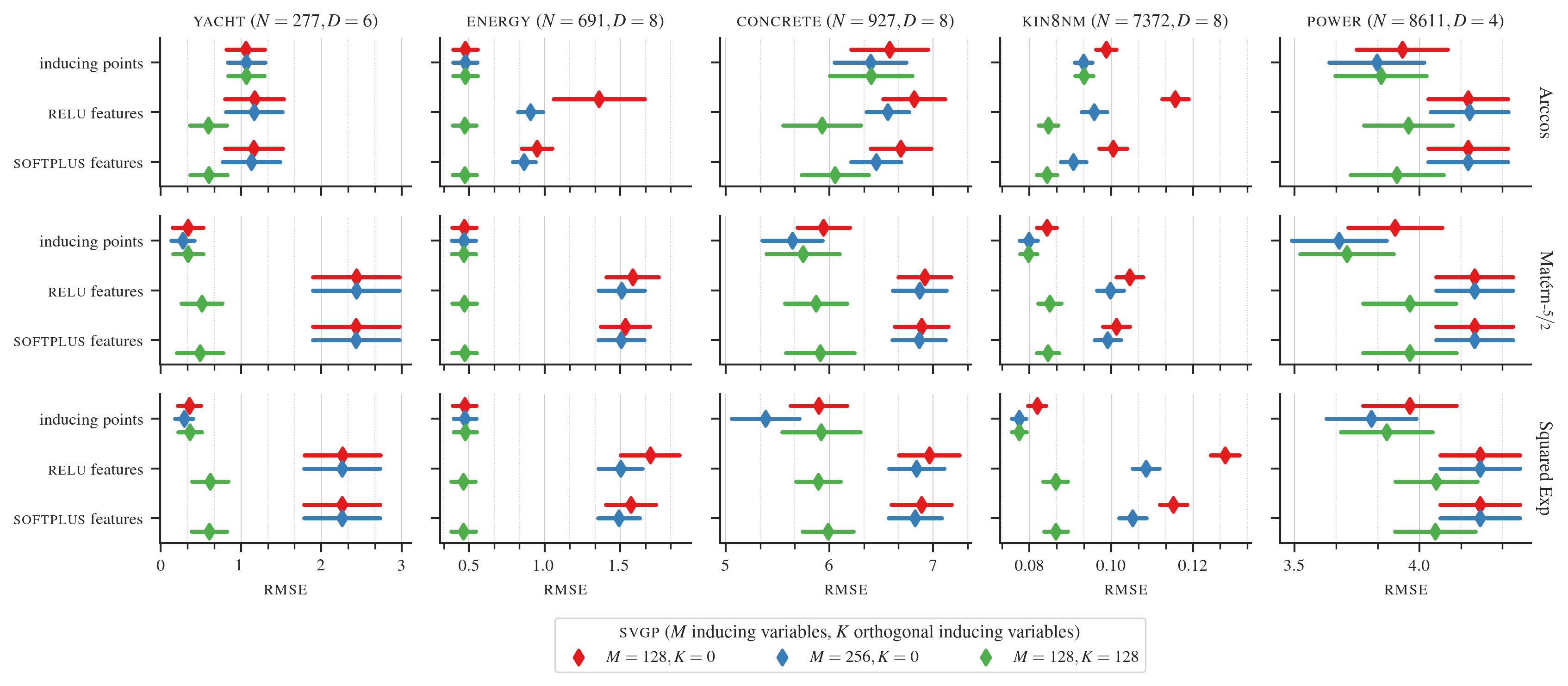
Figure 7: Test rmse on regression problems from the uci repository of datasets for various kernels and activation features. Along the rows labeled “inducing points”, the red and blue markers (${\color[rgb]{0.89453125,0.1015625,0.109375}\blacklozenge},{\color[rgb]{0.21484375,0.4921875,0.72265625}\blacklozenge}$) represent the original svgp model (Titsias, 2009), while the green markers (${\color[rgb]{0.30078125,0.6875,0.2890625}\blacklozenge}$) represent solvegp (Shi et al., 2020). Along the remaining rows, the red and blue markers (${\color[rgb]{0.89453125,0.1015625,0.109375}\blacklozenge},{\color[rgb]{0.21484375,0.4921875,0.72265625}\blacklozenge}$) represent the activated svgp (Dutordoir et al., 2021), while the green markers (${\color[rgb]{0.30078125,0.6875,0.2890625}\blacklozenge}$) represent our proposed approach.

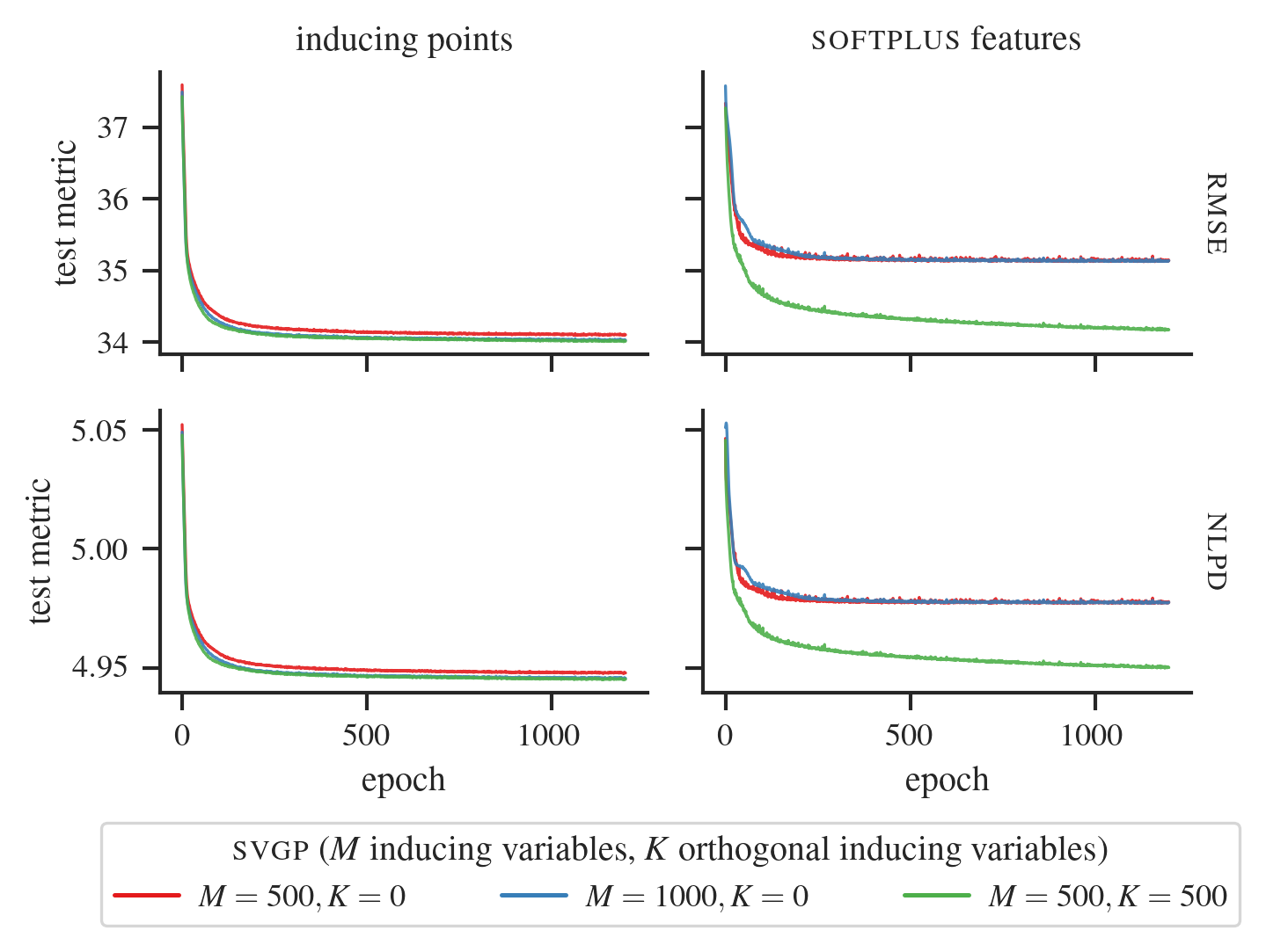
Figure 8: Test metrics, rmse and nlpd, on the large-scale 2008 U.S. airline delays dataset using the Arccos kernel with standard inducing points and softplus-activated features. Along the column labeled “inducing points”, the red and blue lines (— and —) represent the mini-batch svgp (Hensman et al., 2013), while the green line (—) represents solvegp (Shi et al., 2020). Along the column labeled “softplus features”, the red and blue lines (— and —) represent the activated svgp (Dutordoir et al., 2021), while the green line (—) represents our proposed approach.

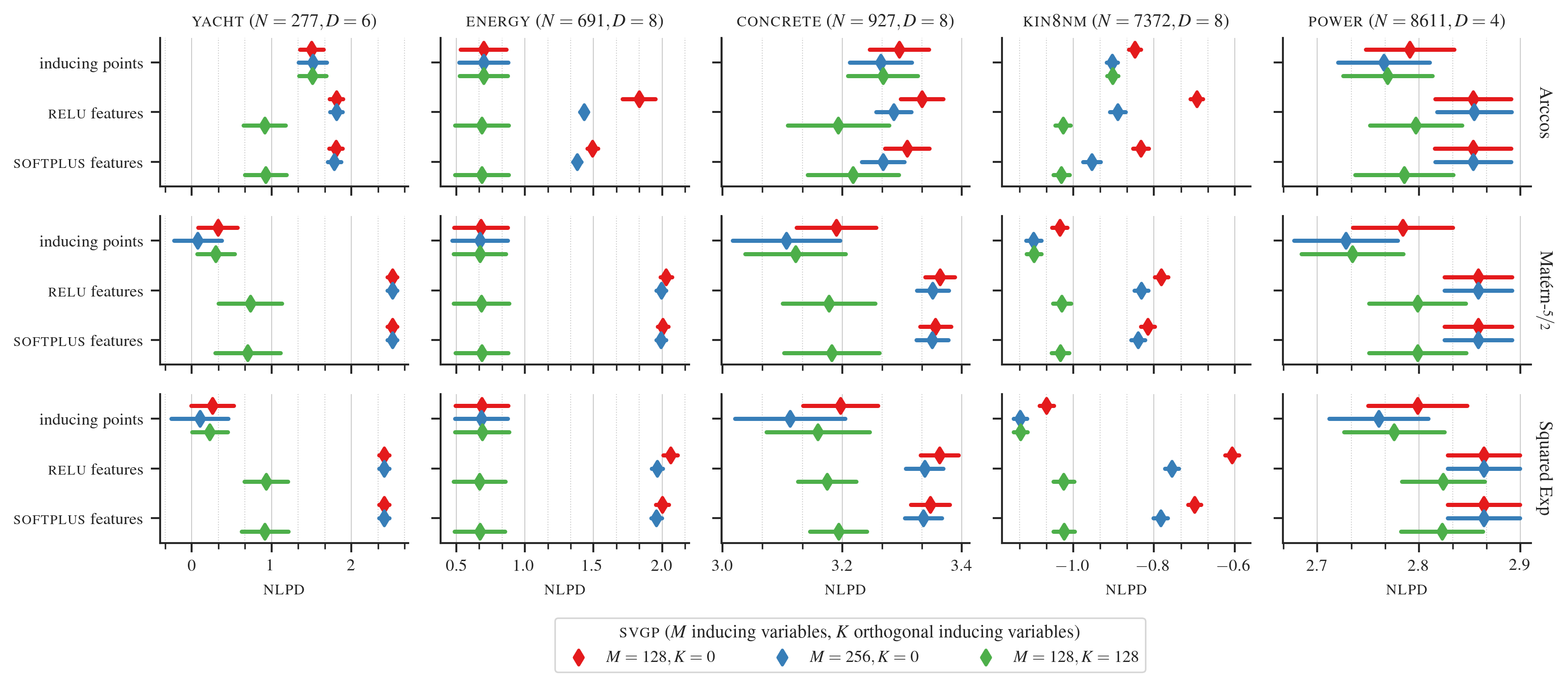
Figure 9: Test nlpd on regression problems from the uci repository of datasets for various kernels and activation features. Along the rows labeled “inducing points”, the red and blue markers (${\color[rgb]{0.89453125,0.1015625,0.109375}\blacklozenge},{\color[rgb]{0.21484375,0.4921875,0.72265625}\blacklozenge}$) represent the original svgp model (Titsias, 2009), while the green markers (${\color[rgb]{0.30078125,0.6875,0.2890625}\blacklozenge}$) represent solvegp (Shi et al., 2020). Along the remaining rows, the red and blue markers (${\color[rgb]{0.89453125,0.1015625,0.109375}\blacklozenge},{\color[rgb]{0.21484375,0.4921875,0.72265625}\blacklozenge}$) represent the activated svgp (Dutordoir et al., 2021), while the green markers (${\color[rgb]{0.30078125,0.6875,0.2890625}\blacklozenge}$) represent our proposed approach.

We observe that, irrespective of the choice of kernel, when using activation features, whether relu- or softplus-activated, augmenting the model with orthogonal bases significantly improves performance, notably even more so than doubling the number of base inducing variables. This can readily be seen across all datasets on both the nlpd and rmse metrics. Further, with the Arccos kernel, it outperforms its counterparts based on standard inducing points across most datasets (the exception being the power dataset). With the Matérn and se kernels, it achieves results comparable to its standard inducing points counterparts in most datasets.

4.3 Large-scale Regression on Airline Delays Dataset

Finally, we consider a large-scale regression dataset concerning U.S. commercial airline delays in 2008. The task is to forecast the duration of delays in reaching the destination of a given flight, utilizing information such as the route distance, airtime, scheduled month, day of the week, and other relevant factors, as well as characteristics of the aircraft such as its age (number of years since deployment). The complete dataset encompasses 5,929,413 flights, of which we randomly select 1M observations without replacement to form a subset that is more manageable but still considerable in scale. Results on a reduced 100K subset can be found in § C.1.

To quantitatively assess performance, we report the test rmse and nlpd evaluated on a $\nicefrac{{1}}{{3}}$ held-out test set. The results are shown in the top and bottom rows of Figure 8, respectively. Within the training set, the inputs and outputs are standardized, i.e. scaled to have zero mean and unit variance and subsequently restored to the original scale at test time.

Given the immense volume of data at hand, we are compelled to utilize mini-batch training for stochastic optimisation (Hensman et al., 2013). To this end, we use the Adam optimizer (Kingma & Ba, 2014) with its typical default settings (learning rate $1\text{\times}{10}^{-3}$, $\beta_{1}=0.9,\beta_{2}=0.999$). Our batch size is set to 5,000, and we train the models for a total of 1,200 epochs.

We fit variations of svgp with the Arccos kernel and (a) standard inducing points and (b) inter-domain inducing features based on softplus-activated inducing features. For each of these variants, we consider three combinations of base and orthogonal inducing variables: (i-ii) 500 and 1,000 base inducing variables (and no orthogonal inducing variables), and (iii) 500 base inducing variables with 500 orthogonal inducing variables. The activation features are truncated at $L=6$ levels. Our proposed method is represented by the combination consisting of softplus-activated features with orthogonal inducing variables (b,iii). The remaining combinations, against which we benchmark, correspond to the mini-batch svgp (a,i-ii) (Hensman et al., 2013), solvegp (a,iii) (Shi et al., 2020), and activated svgp (b,i-ii) (Dutordoir et al., 2021).

The outcomes are as expected when employing standard inducing points (left). In particular, doubling the number of base inducing points from 500 to 1,000 demonstrates significant improvements. Furthermore, by using 500 base inducing points alongside 500 orthogonal inducing points, we achieve comparable performance to having 1,000 base inducing points, while enjoying improved computationally efficiency. In contrast, when examinining the activated svgp model with softplus features (right), it’s apparent that it underperforms compared to the original svgp counterparts. Furthermore, doubling the number of inducing features from 500 to 1,000 has virtually no effect. However, by incorporating orthogonal bases into the activated svgp model with 500 features following our proposed approach, we witness substantial improvements and achieve comparable performance to its standard inducing points counterparts.

5 Conclusion

We considered the use of inter-domain inducing features in the orthogonally-decoupled svgp framework, specifically, the spherical activation features, and showed that this alleviates some of the practical issues and shortcomings associated with the activated svgp model. We demonstrated the effectiveness of this approach by conducting empirical evaluations on several problems, and showed that this leads to enhanced predictive performance over more computationally demanding alternatives such as increasing the truncation levels or the number of inducing variables.

Future work will explore alternative designs of inter-domain inducing features to construct new standard and orthogonal bases that provide additional complementary benefits.

Appendix A Combinations

Recall that the prior over $\mathbf{f},\mathbf{u},\mathbf{v}$ is

$$\begin{bmatrix}\mathbf{f}\\ \mathbf{u}\\ \mathbf{v}\end{bmatrix}\sim\mathcal{N}\left(\begin{bmatrix}\mathbf{0}\\ \mathbf{0}\\ \mathbf{0}\end{bmatrix},\begin{bmatrix}\mathbf{K}_{\mathbf{f}\mathbf{f}}&\mathbf{K}_{\mathbf{u}\mathbf{f}}^{\top}&\mathbf{K}_{\mathbf{v}\mathbf{f}}^{\top}\\ \mathbf{K}_{\mathbf{u}\mathbf{f}}&\mathbf{K}_{\mathbf{u}\mathbf{u}}&\mathbf{K}_{\mathbf{v}\mathbf{u}}^{\top}\\ \mathbf{K}_{\mathbf{v}\mathbf{f}}&\mathbf{K}_{\mathbf{v}\mathbf{u}}&\mathbf{K}_{\mathbf{v}\mathbf{v}}\end{bmatrix}\right)$$ (13)

Other than the variational parameters, the ingredients necessary to compute the predictive for the model described in § 2.4, summarized by Equations 11 and 12, are

$$\mathbf{S}_{\mathbf{f}\mathbf{f}}\triangleq\mathbf{K}_{\mathbf{f}\mathbf{f}}-\mathbf{Q}_{\mathbf{f}\mathbf{f}},\qquad\mathbf{S}_{\mathbf{v}\mathbf{f}}\triangleq\mathbf{K}_{\mathbf{v}\mathbf{f}}-\mathbf{Q}_{\mathbf{v}\mathbf{f}},\qquad\mathbf{S}_{\mathbf{v}\mathbf{v}}\triangleq\mathbf{K}_{\mathbf{v}\mathbf{v}}-\mathbf{Q}_{\mathbf{v}\mathbf{v}},$$

where

$$\mathbf{Q}_{\mathbf{f}\mathbf{f}}\triangleq\mathbf{Q}_{\mathbf{f}\mathbf{u}}\mathbf{K}_{\mathbf{u}\mathbf{u}}\mathbf{Q}_{\mathbf{u}\mathbf{f}},\qquad\mathbf{Q}_{\mathbf{v}\mathbf{f}}\triangleq\mathbf{Q}_{\mathbf{v}\mathbf{u}}\mathbf{K}_{\mathbf{u}\mathbf{u}}\mathbf{Q}_{\mathbf{u}\mathbf{f}},\qquad\mathbf{Q}_{\mathbf{v}\mathbf{v}}\triangleq\mathbf{Q}_{\mathbf{v}\mathbf{u}}\mathbf{K}_{\mathbf{u}\mathbf{u}}\mathbf{Q}_{\mathbf{u}\mathbf{v}},$$

and

$$\mathbf{Q}_{\mathbf{f}\mathbf{u}}\triangleq\mathbf{K}_{\mathbf{f}\mathbf{u}}\mathbf{K}_{\mathbf{u}\mathbf{u}}^{-1},\qquad\mathbf{Q}_{\mathbf{v}\mathbf{u}}\triangleq\mathbf{K}_{\mathbf{v}\mathbf{u}}\mathbf{K}_{\mathbf{u}\mathbf{u}}^{-1}.$$

In all the cases we shall discuss below, $\mathbf{K}_{\mathbf{f}\mathbf{f}}$ will evaluate to

$$\left[\mathbf{K}_{\mathbf{f}\mathbf{f}}\right]_{nn^{\prime}}=\mathrm{Cov}\left(f(\mathbf{x}_{n}),f(\mathbf{x}_{n^{\prime}})\right)=\langle k(\mathbf{x}_{n},\cdot\,),k(\mathbf{x}_{n^{\prime}},\cdot\,)\rangle_{\mathcal{H}}=k(\mathbf{x}_{n},\mathbf{x}_{n^{\prime}}).$$ (14)

Similarly, $\mathbf{K}_{\mathbf{u}\mathbf{f}}$ and $\mathbf{K}_{\mathbf{v}\mathbf{f}}$ will always simplify to

$$\left[\mathbf{K}_{\mathbf{u}\mathbf{f}}\right]_{mn} =\mathrm{Cov}\left(u_{m},f(\mathbf{x}_{n})\right)=\langle\phi_{m},k(\mathbf{x}_{n},\cdot\,)\rangle_{\mathcal{H}}=\phi_{m}(\mathbf{x}_{n})$$ (15)

$$\left[\mathbf{K}_{\mathbf{v}\mathbf{f}}\right]_{kn} =\mathrm{Cov}\left(v_{k},f(\mathbf{x}_{n})\right)=\langle\psi_{k},k(\mathbf{x}_{n},\cdot\,)\rangle_{\mathcal{H}}=\psi_{k}(\mathbf{x}_{n})$$ (16)

The remaining covariances $\mathbf{K}_{\mathbf{u}\mathbf{u}},\mathbf{K}_{\mathbf{v}\mathbf{u}}$ and $\mathbf{K}_{\mathbf{v}\mathbf{v}}$ reduce to different forms, depending on the choices of $\phi_{m}$ and $\psi_{k}$,

$$\left[\mathbf{K}_{\mathbf{u}\mathbf{u}}\right]_{mm^{\prime}} =\mathrm{Cov}\left(u_{m},u_{m^{\prime}}\right)=\langle\phi_{m},\phi_{m^{\prime}}\rangle_{\mathcal{H}},$$ (17)

$$\left[\mathbf{K}_{\mathbf{v}\mathbf{u}}\right]_{km} =\mathrm{Cov}\left(v_{k},u_{m}\right)=\langle\psi_{k},\phi_{m}\rangle_{\mathcal{H}},$$ (18)

$$\left[\mathbf{K}_{\mathbf{v}\mathbf{v}}\right]_{kk^{\prime}} =\mathrm{Cov}\left(v_{k},v_{k^{\prime}}\right)=\langle\psi_{k},\psi_{k^{\prime}}\rangle_{\mathcal{H}}.$$ (19)

In general, we have

$$\left[\mathbf{Q}_{\mathbf{v}\mathbf{f}}\right]_{kn}=\sum_{\begin{subarray}{c}m=1,\\ m^{\prime}=1\end{subarray}}^{M}\left[\mathbf{K}_{\mathbf{u}\mathbf{u}}^{-1}\right]_{mm^{\prime}}\langle\psi_{k},\phi_{m}\rangle_{\mathcal{H}}\langle\phi_{m^{\prime}},k(\mathbf{x}_{n},\cdot)\rangle_{\mathcal{H}},$$ (20)

and

$$\left[\mathbf{Q}_{\mathbf{v}\mathbf{v}}\right]_{kk^{\prime}}=\sum_{\begin{subarray}{c}m=1,\\ m^{\prime}=1\end{subarray}}^{M}\left[\mathbf{K}_{\mathbf{u}\mathbf{u}}^{-1}\right]_{mm^{\prime}}\langle\psi_{k},\phi_{m}\rangle_{\mathcal{H}}\langle\phi_{m^{\prime}},\psi_{k^{\prime}}\rangle_{\mathcal{H}}$$ (21)

We enumerate the combinations in turn and discuss their benefits and drawbacks.

A.1 Base Inducing Variables as Standard Inducing Points

In this case, the base inducing variables are simply standard inducing points $u_{m}=f(\mathbf{z}_{m})$, which is equivalent to defining $\phi_{m}:\mathbf{x}\mapsto k(\mathbf{z}_{m},\mathbf{x})$. Therefore, we have

$$\left[\mathbf{K}_{\mathbf{u}\mathbf{f}}\right]_{mn} =\phi_{m}(\mathbf{x}_{n})=k(\mathbf{z}_{m},\mathbf{x}_{n}),$$ (22)

$$\left[\mathbf{K}_{\mathbf{u}\mathbf{u}}\right]_{mm^{\prime}} =\langle\phi_{m},\phi_{m^{\prime}}\rangle_{\mathcal{H}}=\langle k(\mathbf{z}_{m},\cdot\,),k(\mathbf{z}_{m^{\prime}},\cdot\,)\rangle_{\mathcal{H}}=k(\mathbf{z}_{m},\mathbf{z}_{m^{\prime}}).$$ (23)

A.1.1 Orthogonal Inducing Variables as Standard Inducing Points

In this case, the orthogonal inducing variables are simply standard inducing points $v_{k}=f(\mathbf{w}_{m})$, which is equivalent to defining $\psi_{k}:\mathbf{x}\mapsto k(\mathbf{w}_{k},\mathbf{x})$. Note that this combination is precisely the original method of Shi et al. (2020). Hence, we have

$$\left[\mathbf{K}_{\mathbf{v}\mathbf{f}}\right]_{kn} =\psi_{k}(\mathbf{x}_{n})=k(\mathbf{w}_{k},\mathbf{x}_{n}),$$ (24)

$$\left[\mathbf{K}_{\mathbf{v}\mathbf{u}}\right]_{km} =\langle\psi_{k},\phi_{m}\rangle_{\mathcal{H}}=\langle k(\mathbf{w}_{k},\cdot\,),k(\mathbf{z}_{m},\cdot\,)\rangle_{\mathcal{H}}=k(\mathbf{w}_{k},\mathbf{z}_{m}),$$ (25)

$$\left[\mathbf{K}_{\mathbf{v}\mathbf{v}}\right]_{kk^{\prime}} =\langle\psi_{k},\psi_{k^{\prime}}\rangle_{\mathcal{H}}=\langle k(\mathbf{w}_{k},\cdot\,),k(\mathbf{w}_{k^{\prime}},\cdot\,))\rangle_{\mathcal{H}}=k(\mathbf{w}_{k},\mathbf{w}_{k^{\prime}}).$$ (26)

This leads to

$$\left[\mathbf{Q}_{\mathbf{v}\mathbf{f}}\right]_{kn}=\sum_{m=1}^{M}\sum_{m^{\prime}=1}^{M}\left[\mathbf{K}_{\mathbf{u}\mathbf{u}}^{-1}\right]_{mm^{\prime}}k(\mathbf{w}_{k},\mathbf{z}_{m})k(\mathbf{z}_{m^{\prime}},\mathbf{x}_{n}),$$ (27)

and $\mathbf{S}_{\mathbf{v}\mathbf{f}}$ does not simplify further.

A.1.2 Orthogonal Inducing Variables as Spherical Harmonics

Here, orthogonal inducing variables are defined through inter-domain features $v_{k}=\langle f,\psi_{k}\rangle_{\mathcal{H}}$ where $\psi_{k}\triangleq{Y}_{\ell,j}$, the spherical harmonic of level $\ell$ and order $j$, and $k$ indexes the pairs $(\ell,j)$. Hence, $\mathbf{K}_{\mathbf{v}\mathbf{f}}$ is as expressed in Equation 16,

$$\left[\mathbf{K}_{\mathbf{v}\mathbf{u}}\right]_{km} =\langle\psi_{k},\phi_{m}\rangle_{\mathcal{H}}=\langle\psi_{k},k(\mathbf{z}_{m},\cdot\,)\rangle_{\mathcal{H}}=\psi_{k}(\mathbf{z}_{m})$$ (28)

$$\left[\mathbf{K}_{\mathbf{v}\mathbf{v}}\right]_{kk^{\prime}} =\langle\psi_{k},\psi_{k^{\prime}}\rangle_{\mathcal{H}}=\lambda_{k}^{-1}\delta_{kk^{\prime}}$$ (29)

This leads to

$$\left[\mathbf{Q}_{\mathbf{v}\mathbf{f}}\right]_{kn}=\sum_{m=1}^{M}\sum_{m^{\prime}=1}^{M}\left[\mathbf{K}_{\mathbf{u}\mathbf{u}}^{-1}\right]_{mm^{\prime}}\psi_{k}(\mathbf{z}_{m})k(\mathbf{z}_{m^{\prime}},\mathbf{x}_{n})$$ (30)

and $\mathbf{S}_{\mathbf{v}\mathbf{f}}$ does not simplify further.

A.1.3 Orthogonal Inducing Variables as Spherical NN Activations

Here, orthogonal inducing variables are defined through inter-domain features $v_{k}=\langle f,\psi_{k}\rangle_{\mathcal{H}}$ where $\psi_{k}=H_{k}$, the $k$-th unit of a spherical nn activation layer (Equation 6). Again, $\mathbf{K}_{\mathbf{v}\mathbf{f}}$ is as expressed in Equation 16, and we still get $\left[\mathbf{K}_{\mathbf{v}\mathbf{u}}\right]_{km}=\psi_{k}(\mathbf{z}_{m})$ as in Equation 28 from the preceding case, but we now have

$$\left[\mathbf{K}_{\mathbf{v}\mathbf{v}}\right]_{kk^{\prime}}=\langle\psi_{k},\psi_{k^{\prime}}\rangle_{\mathcal{H}}=\sum_{\begin{subarray}{c}\ell=0:\\ \lambda_{\ell}\neq 0\end{subarray}}^{\infty}\frac{\varsigma_{\ell}^{2}}{\lambda_{\ell}}\frac{\ell+\alpha}{\alpha}C_{\ell}^{(\alpha)}\left(\frac{\mathbf{w}_{k}^{\top}\mathbf{w}_{k^{\prime}}}{\lVert\mathbf{w}_{k}\rVert\lVert\mathbf{w}_{k^{\prime}}\rVert}\right),$$ (31)

which leads to

$$\left[\mathbf{Q}_{\mathbf{v}\mathbf{f}}\right]_{kn}=\sum_{m=1}^{M}\sum_{m^{\prime}=1}^{M}\left[\mathbf{K}_{\mathbf{u}\mathbf{u}}^{-1}\right]_{mm^{\prime}}\psi_{k}(\mathbf{z}_{m})k(\mathbf{z}_{m^{\prime}},\mathbf{x}_{n}).$$ (32)

and $\mathbf{S}_{\mathbf{v}\mathbf{f}}$ does not simplify further.

A.2 Base Inducing Variables as Spherical Harmonics

Here, the base inducing variables are defined through inter-domain features $u_{m}=\langle f,\phi_{m}\rangle_{\mathcal{H}}$ where $\phi_{m}\triangleq{Y}_{\ell,j}$, the spherical harmonic of level $\ell$ and order $j$, and $m$ indexes the pairs $(\ell,j)$. In this case, $\left[\mathbf{K}_{\mathbf{u}\mathbf{f}}\right]_{mn}=\phi_{m}(\mathbf{x}_{n})$ as in Equation 15, and

$$\left[\mathbf{K}_{\mathbf{u}\mathbf{u}}\right]_{mm^{\prime}}=\langle\phi_{m},\phi_{m^{\prime}}\rangle_{\mathcal{H}}=\lambda_{m}^{-1}\delta_{mm^{\prime}}.$$ (33)

Therefore, we can already simplify $\mathbf{Q}_{\mathbf{v}\mathbf{f}}$ from Equation 20 as

$$\left[\mathbf{Q}_{\mathbf{v}\mathbf{f}}\right]_{kn}=\sum_{m=1}^{M}\sum_{m^{\prime}=1}^{M}\delta_{mm^{\prime}}\lambda_{m}\langle\psi_{k},\phi_{m}\rangle_{\mathcal{H}}\phi_{m^{\prime}}(\mathbf{x}_{n})=\sum_{m=1}^{M}\lambda_{m}\langle\psi_{k},\phi_{m}\rangle_{\mathcal{H}}\phi_{m}(\mathbf{x}_{n})$$ (34)

A.2.1 Orthogonal Inducing Variables as Standard Inducing Points

In this case, the orthogonal inducing variables are simply standard inducing points $v_{k}=f(\mathbf{w}_{m})$, which is equivalent to defining $\psi_{k}:\mathbf{x}\mapsto k(\mathbf{w}_{k},\mathbf{x})$. Hence, we have

$$\left[\mathbf{K}_{\mathbf{v}\mathbf{f}}\right]_{kn} =\psi_{k}(\mathbf{x}_{n})=k(\mathbf{w}_{k},\mathbf{x}_{n})$$ (35)

$$\left[\mathbf{K}_{\mathbf{v}\mathbf{u}}\right]_{km} =\langle\psi_{k},\phi_{m}\rangle_{\mathcal{H}}=\langle k(\mathbf{w}_{k},\cdot\,),\phi_{m}\rangle_{\mathcal{H}}=\phi_{m}(\mathbf{w}_{k})$$ (36)

$$\left[\mathbf{K}_{\mathbf{v}\mathbf{v}}\right]_{kk^{\prime}} =\langle\psi_{k},\psi_{k^{\prime}}\rangle_{\mathcal{H}}=\langle k(\mathbf{w}_{k},\cdot\,),k(\mathbf{w}_{k^{\prime}},\cdot\,))\rangle_{\mathcal{H}}=k(\mathbf{w}_{k},\mathbf{w}_{k^{\prime}})$$ (37)

Carrying on from Equation 34,

$$\left[\mathbf{Q}_{\mathbf{v}\mathbf{f}}\right]_{kn} =\sum_{m=1}^{M}\lambda_{m}\phi_{m}(\mathbf{w}_{k})\phi_{m}(\mathbf{x}_{n})=\sum_{\ell=1}^{L}\sum_{j=1}^{J_{\ell}^{d}}\lambda_{\ell,j}{Y}_{\ell,j}(\mathbf{w}_{k}){Y}_{\ell,j}(\mathbf{x}_{n}).$$ (38)

Now, as $M\to\infty$ (more precisely, as $L\to\infty$), $\left[\mathbf{Q}_{\mathbf{v}\mathbf{f}}\right]_{kn}$ converges to $k(\mathbf{w}_{k},\mathbf{x}_{n})=\left[\mathbf{K}_{\mathbf{v}\mathbf{f}}\right]_{kn}$. In other words, $\left[\mathbf{S}_{\mathbf{v}\mathbf{f}}\right]_{kn}$ approaches zero in the limit, and the orthogonal component of the variational parameterization vanishes, effectively reducing this combination to standard svgp. However, for finite $M$, particularly the modest values that are feasible in practice, the orthogonal component remains and will strictly improve the modelling capacity by capturing the residues that the base component cannot.

A.2.2 Orthogonal Inducing Variables as Spherical Harmonics

Here, orthogonal inducing variables are defined through inter-domain features $v_{k}=\langle f,\psi_{k}\rangle_{\mathcal{H}}$ where $\psi_{k}\triangleq{Y}_{\ell,j}$, the spherical harmonic of level $\ell$ and order $j$, and $k$ indexes the pairs $(\ell,j)$. Hence, $\mathbf{K}_{\mathbf{v}\mathbf{f}}$ is as expressed in Equation 16, and

$$\left[\mathbf{K}_{\mathbf{v}\mathbf{u}}\right]_{km} =\langle\psi_{k},\phi_{m}\rangle_{\mathcal{H}}=\lambda_{m}^{-1}\delta_{mk}$$ (39)

$$\left[\mathbf{K}_{\mathbf{v}\mathbf{v}}\right]_{kk^{\prime}} =\langle\psi_{k},\psi_{k^{\prime}}\rangle_{\mathcal{H}}=\lambda_{k}^{-1}\delta_{kk^{\prime}}$$ (40)

This leads to

$$\left[\mathbf{Q}_{\mathbf{v}\mathbf{f}}\right]_{kn}=\sum_{m=1}^{M}\lambda_{m}\langle\psi_{k},\phi_{m}\rangle_{\mathcal{H}}\phi_{m}(\mathbf{x}_{n})=\sum_{m=1}^{M}\delta_{mk}\phi_{m}(\mathbf{x}_{n})=\phi_{k}(\mathbf{x}_{n})$$ (41)

in this case, since $\psi_{k}=\phi_{k}$, we have $\left[\mathbf{S}_{\mathbf{v}\mathbf{f}}\right]_{kn}=0$ and this approach collapses to standard svgp, regardless of the value of $M$.

A.2.3 Orthogonal Inducing Variables as Spherical NN Activations

Here, orthogonal inducing variables are defined through inter-domain features $v_{k}=\langle f,\psi_{k}\rangle_{\mathcal{H}}$ where $\psi_{k}=H_{k}$, the $k$-th unit of a spherical nn activation layer (Equation 6). Again, $\mathbf{K}_{\mathbf{v}\mathbf{f}}$ is as expressed in Equation 16, and we now have

$$\left[\mathbf{K}_{\mathbf{v}\mathbf{u}}\right]_{km} =\langle\psi_{k},\phi_{m}\rangle_{\mathcal{H}}=\lambda_{m}^{-1}\varsigma_{m}\phi_{m}(\mathbf{w}_{k})$$ (42)

$$\left[\mathbf{K}_{\mathbf{v}\mathbf{v}}\right]_{kk^{\prime}} =\langle\psi_{k},\psi_{k^{\prime}}\rangle_{\mathcal{H}}=\sum_{\begin{subarray}{c}\ell=0:\\ \lambda_{\ell}\neq 0\end{subarray}}^{\infty}\frac{\varsigma_{\ell}^{2}}{\lambda_{\ell}}\frac{\ell+\alpha}{\alpha}C_{\ell}^{(\alpha)}\left(\frac{\mathbf{w}_{k}^{\top}\mathbf{w}_{k^{\prime}}}{\lVert\mathbf{w}_{k}\rVert\lVert\mathbf{w}_{k^{\prime}}\rVert}\right)$$ (43)

which leads to

$$\left[\mathbf{Q}_{\mathbf{v}\mathbf{f}}\right]_{kn}=\sum_{m=1}^{M}\varsigma_{m}\phi_{m}(\mathbf{w}_{k})\phi_{m}(\mathbf{x}_{n})$$ (44)

Similar to § A.2.1, as $M\to\infty$ (more precisely, as $L\to\infty$), $\left[\mathbf{Q}_{\mathbf{v}\mathbf{f}}\right]_{kn}$ converges to $\psi_{k}(\mathbf{x}_{n})=\left[\mathbf{K}_{\mathbf{v}\mathbf{f}}\right]_{kn}$. So again, $\left[\mathbf{S}_{\mathbf{v}\mathbf{f}}\right]_{kn}$ approaches zero in the limit, and the orthogonal component of the variational parameterization vanishes, effectively reducing this combination to standard svgp. However, for finite $M$, particularly the small values that are feasible in practice, the orthogonal component remains and will strictly improve the modelling capacity by capturing the residues that the base component cannot.

A.3 Base Inducing Variables as Spherical NN Activations

Here, the base inducing variables are defined through inter-domain features $u_{m}=\langle f,\phi_{m}\rangle_{\mathcal{H}}$ where $\phi_{m}=H_{m}$, the $m$-th unit of a spherical nn activation layer (Equation 6).

In this case, $\left[\mathbf{K}_{\mathbf{u}\mathbf{f}}\right]_{mn}=\phi_{m}(\mathbf{x}_{n})$ as in Equation 15, and

$$\left[\mathbf{K}_{\mathbf{u}\mathbf{u}}\right]_{mm^{\prime}}=\langle\phi_{m},\phi_{m^{\prime}}\rangle_{\mathcal{H}}=\sum_{\ell=0:\lambda_{\ell}\neq 0}^{\infty}\frac{\varsigma_{\ell}^{2}}{\lambda_{\ell}}\frac{\ell+\alpha}{\alpha}C_{\ell}^{(\alpha)}\left(\frac{\mathbf{z}_{m}^{\top}\mathbf{z}_{m^{\prime}}}{\lVert\mathbf{z}_{m}\rVert\lVert\mathbf{z}_{m^{\prime}}\rVert}\right)$$ (45)

A.3.1 Orthogonal Inducing Variables as Standard Inducing Points

In this case, the orthogonal inducing variables are simply standard inducing points $v_{k}=f(\mathbf{w}_{m})$, which is equivalent to defining $\psi_{k}:\mathbf{x}\mapsto k(\mathbf{w}_{k},\mathbf{x})$. Hence, we have

$$\left[\mathbf{K}_{\mathbf{v}\mathbf{f}}\right]_{kn} =\psi_{k}(\mathbf{x}_{n})=k(\mathbf{w}_{k},\mathbf{x}_{n})$$ (46)

$$\left[\mathbf{K}_{\mathbf{v}\mathbf{u}}\right]_{km} =\langle\psi_{k},\phi_{m}\rangle_{\mathcal{H}}=\langle k(\mathbf{w}_{k},\cdot\,),\phi_{m}\rangle_{\mathcal{H}}=\phi_{m}(\mathbf{w}_{k})$$ (47)

$$\left[\mathbf{K}_{\mathbf{v}\mathbf{v}}\right]_{kk^{\prime}} =\langle\psi_{k},\psi_{k^{\prime}}\rangle_{\mathcal{H}}=\langle k(\mathbf{w}_{k},\cdot\,),k(\mathbf{w}_{k^{\prime}},\cdot\,))\rangle_{\mathcal{H}}=k(\mathbf{w}_{k},\mathbf{w}_{k^{\prime}})$$ (48)

as in § A.2.1.

A.3.2 Orthogonal Inducing Variables as Spherical Harmonics

Here, orthogonal inducing variables are defined through inter-domain features $v_{k}=\langle f,\psi_{k}\rangle_{\mathcal{H}}$ where $\psi_{k}=H_{k}$, the $k$-th unit of a spherical nn activation layer (Equation 6).

We have

$$\left[\mathbf{K}_{\mathbf{v}\mathbf{u}}\right]_{km} =\langle\psi_{k},\phi_{m}\rangle_{\mathcal{H}}=\lambda_{k}^{-1}\varsigma_{k}\psi_{k}(\mathbf{z}_{m})$$ (49)

$$\left[\mathbf{K}_{\mathbf{v}\mathbf{f}}\right]_{kn} =\langle\psi_{k},f(\mathbf{x}_{n})\rangle_{\mathcal{H}}=\langle\psi_{k},k(\mathbf{x}_{n},\cdot\,)\rangle_{\mathcal{H}}=\psi_{k}(\mathbf{x}_{n})$$ (50)

$$\left[\mathbf{K}_{\mathbf{v}\mathbf{v}}\right]_{kk^{\prime}} =\langle\psi_{k},\psi_{k^{\prime}}\rangle_{\mathcal{H}}=\lambda_{k}^{-1}\delta_{kk^{\prime}}$$ (51)

This leads to

$$\left[\mathbf{Q}_{\mathbf{v}\mathbf{f}}\right]_{kn}=\sum_{m=1}^{M}\sum_{m^{\prime}=1}^{M}\left[\mathbf{K}_{\mathbf{u}\mathbf{u}}^{-1}\right]_{mm^{\prime}}\lambda_{k}^{-1}\varsigma_{k}\psi_{k}(\mathbf{z}_{m})\phi_{m^{\prime}}(\mathbf{x}_{n})$$ (52)

A.3.3 Orthogonal Inducing Variables as Spherical NN Activations

Here, orthogonal inducing variables are defined through inter-domain features $v_{k}=\langle f,\psi_{k}\rangle_{\mathcal{H}}$ where $\psi_{k}=H_{k}$, the $k$-th unit of a spherical nn activation layer (Equation 6).

In this case, we still get

$$\left[\mathbf{K}_{\mathbf{v}\mathbf{u}}\right]_{km} =\langle\psi_{k},\phi_{m}\rangle_{\mathcal{H}}=\sum_{\ell=0:\lambda_{\ell}\neq 0}^{\infty}\frac{\varsigma_{\ell}^{2}}{\lambda_{\ell}}\frac{\ell+\alpha}{\alpha}C_{\ell}^{(\alpha)}\left(\frac{\mathbf{w}_{k}^{\top}\mathbf{z}_{m}}{\lVert\mathbf{w}_{k}\rVert\lVert\mathbf{z}_{m}\rVert}\right)$$ (53)

$$\left[\mathbf{K}_{\mathbf{v}\mathbf{f}}\right]_{kn} =\langle\psi_{k},f(\mathbf{x}_{n})\rangle_{\mathcal{H}}=\langle\psi_{k},k(\mathbf{x}_{n},\cdot\,)\rangle_{\mathcal{H}}=\psi_{k}(\mathbf{x}_{n})$$ (54)

$$\left[\mathbf{K}_{\mathbf{v}\mathbf{v}}\right]_{kk^{\prime}} =\langle\psi_{k},\psi_{k^{\prime}}\rangle_{\mathcal{H}}=\sum_{\ell=0:\lambda_{\ell}\neq 0}^{\infty}\frac{\varsigma_{\ell}^{2}}{\lambda_{\ell}}\frac{\ell+\alpha}{\alpha}C_{\ell}^{(\alpha)}\left(\frac{\mathbf{w}_{k}^{\top}\mathbf{w}_{k^{\prime}}}{\lVert\mathbf{w}_{k}\rVert\lVert\mathbf{w}_{k^{\prime}}\rVert}\right)$$ (55)

Appendix B Experimental Set-up and Implementation Details

B.1 Hardware

All experiments were carried out on a consumer-grade laptop computer with an Intel Core™ i7-11800H (8 Cores) @ 4.6GHz Processor, 16GB Memory, and a NVIDIA GeForce RTX™ 3070 Laptop (Mobile/Max-Q) Graphics Card.

B.2 Software

Our method is implemented by extending functionality from the GPFlow software library (Matthews et al., 2017). The code will be released as open-source software upon publication. Additional software dependencies upon which our implementation relies, either directly or indirectly, are enumerated in Table 2.

Table 2: Key software dependencies.

Method	Software Library	URL (github.com/*)
svgp (Titsias, 2009)	GPFlow	GPflow/GPflow
odvgp (Salimbeni et al., 2018)	-	hughsalimbeni/orth_decoupled_var_gps
solvegp (Shi et al., 2020)	-	thjashin/solvegp
vish (Dutordoir et al., 2020)	Spherical Harmonics	vdutor/SphericalHarmonics
activated svgp (Dutordoir et al., 2021)	-	vdutor/ActivatedDeepGPs
-	Bayesian Benchmarks	hughsalimbeni/bayesian_benchmarks

B.3 Hyperparameters

We adopt sensible defaults across all problems and datasets; no hand-tuning is applied to any specific one. The choices of the hyperparameters and other relevant dependencies are summarized as follows:

Optimization.  We use the l-bfgs optimizer (Byrd et al., 1995; Zhu et al., 1997) with the default settings from scipy.optimize (Virtanen et al., 2020).

Likelihood.  The Gaussian likelihood variance is initialized to 1.0 across all experiments.

Kernel parameter initialization.  All stationary kernels are initialized with unit lengthscale and amplitude.

Variational parameter initialization.  The variational distributions $q(\mathbf{u})$, $q(\mathbf{v}^{\prime})$ are initialized with zero mean and identity covariance $\mathbf{m}=\mathbf{0},\mathbf{C}=\mathbf{I}$.

Whitened parameterization.  We do not use the whitened parameterization (as used, for example, by Murray & Adams (2010); Hensman et al. (2015b)) in either $q(\mathbf{u})$ or $q(\mathbf{v}^{\prime})$.

Inducing point initialization.  We make our best effort to ensure a fair comparison against baselines involving standard inducing points. To this end, we adopt the best practice of first optimizing the variational parameters, not least the inducing input locations $\mathbf{Z}$ (and $\mathbf{W}$ where applicable), before jointly optimizing all of the free parameters. This initialization phase is done for up to 100 iterations of the l-bfgs algorithm.

Appendix C Additional Results

C.1 Regression on Airline Delays Dataset

We repeat the experiment outlined in § 4.3, focusing on a reduced subset of the 2008 U.S. airline delays dataset that consists of 100K randomly selected observations. Unlike the previous experimental set-up, the parameters are optimised for a total of 1,000 epochs. Additionally, we report aggregated results from 5 repetitions across $\nicefrac{{1}}{{3}}$ held-out test sets. The results are shown in Figure 10.

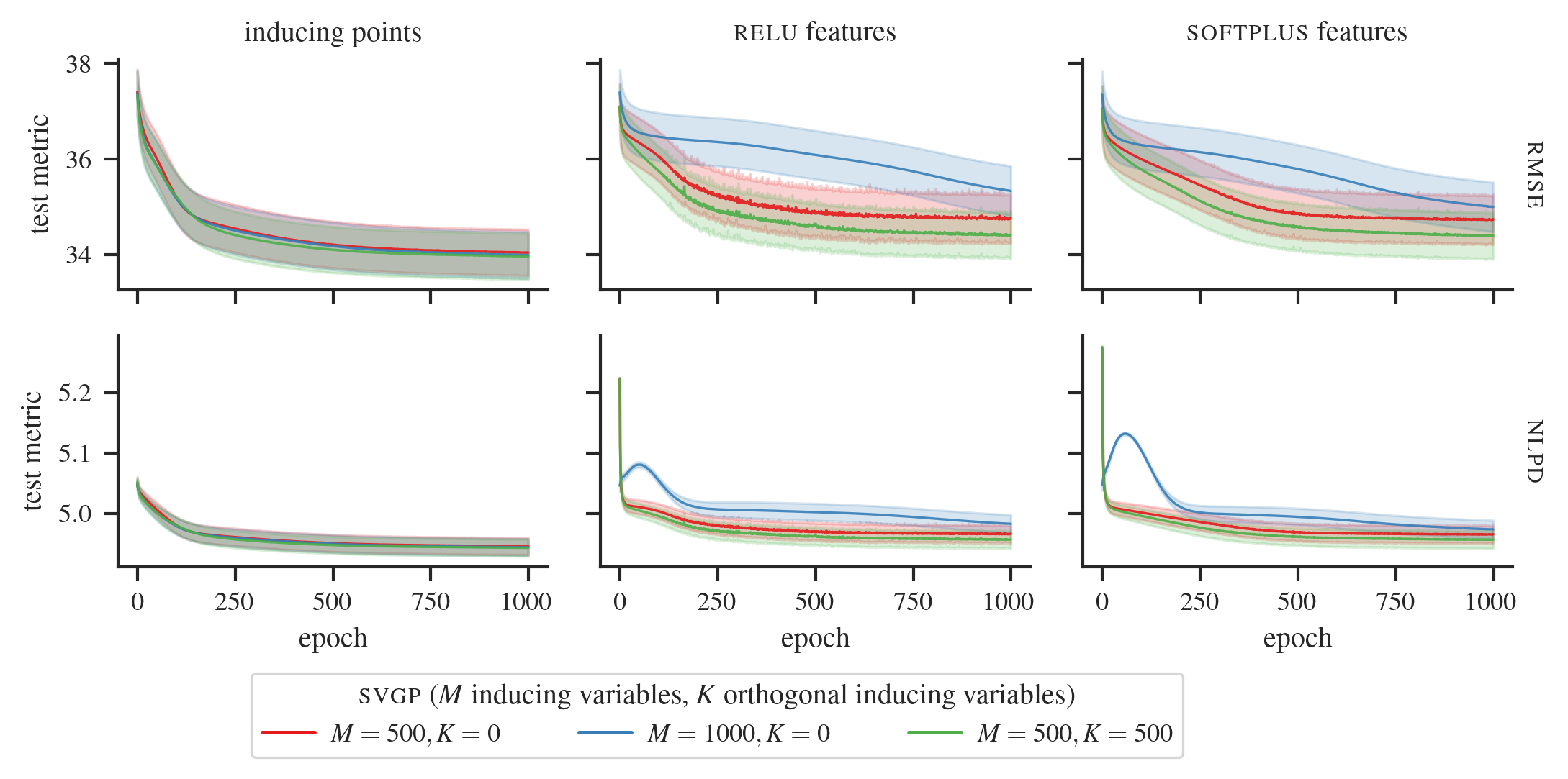
Figure 10: Test metrics, rmse and nlpd, aggregated across 5 random sub-sampling test splits on a 100K subset of the 2008 U.S. airline delays dataset. Results are shown for models using the Arccos kernel with standard inducing points and various activation features. Along the column labeled “inducing points”, the red and blue lines (— and —) represent the mini-batch svgp (Hensman et al., 2013), while the green line (—) represents solvegp (Shi et al., 2020). Along the column labeled “softplus features”, the red and blue lines (— and —) represent the activated svgp (Dutordoir et al., 2021), while the green line (—) represents our proposed approach.

C.2 Extra UCI Repository Datasets

Results on a few larger regression datasets from the uci repository can be found in Figure 11. In this analysis, we adopted the same combination of activation features and sparse gp models as described in § 4.2. However, in contrast to § 4.2, we restrict our focus to the Arccos kernel.

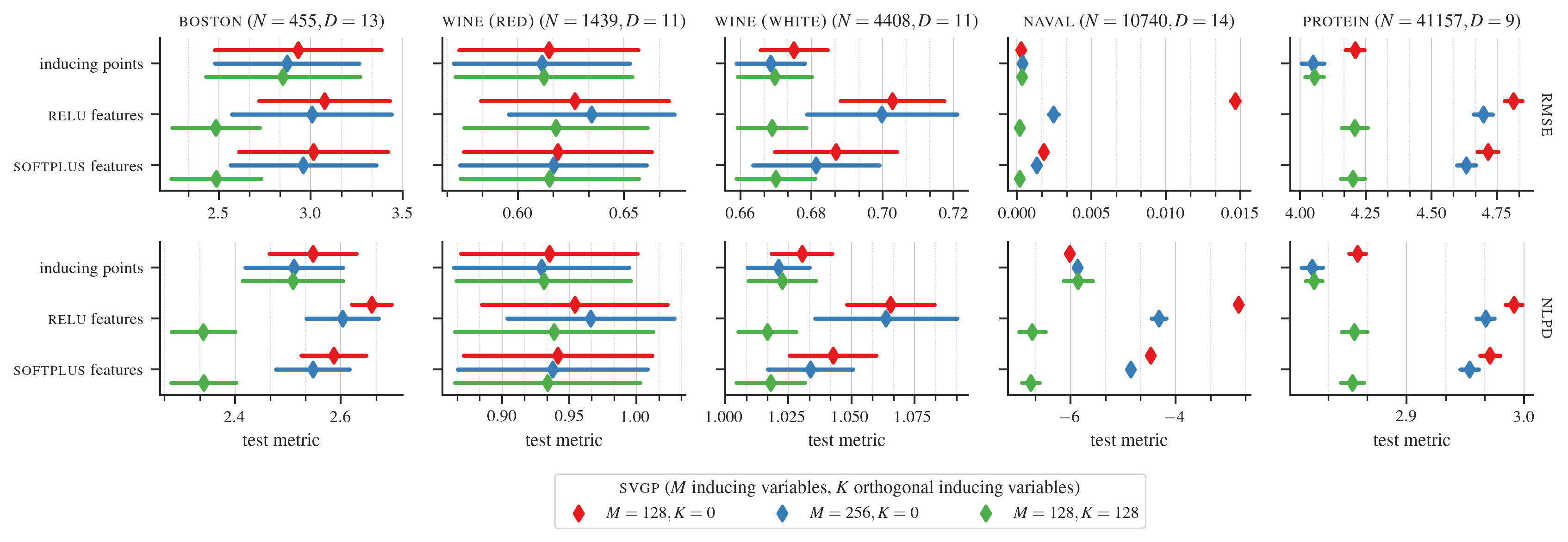
Figure 11: Test metrics, rmse and nlpd, on an extra set of larger regression problems from the uci dataset repository for the Arccos kernel and various activation features. Along the rows labeled “inducing points”, the red and blue markers (${\color[rgb]{0.89453125,0.1015625,0.109375}\blacklozenge},{\color[rgb]{0.21484375,0.4921875,0.72265625}\blacklozenge}$) represent the original svgp model (Titsias, 2009), while the green markers (${\color[rgb]{0.30078125,0.6875,0.2890625}\blacklozenge}$) represent solvegp (Shi et al., 2020). Along the remaining rows, the red and blue markers (${\color[rgb]{0.89453125,0.1015625,0.109375}\blacklozenge},{\color[rgb]{0.21484375,0.4921875,0.72265625}\blacklozenge}$) represent the activated svgp (Dutordoir et al., 2021), while the green markers (${\color[rgb]{0.30078125,0.6875,0.2890625}\blacklozenge}$) represent our proposed approach.

C.3 Numerical Tables

For completeness, we include the numerical values of underlying Figures 7 and 9 from § 4 in Tables 3 and 4 below.

Table 3: Numerical values of the test rmse corresponding to Figure 7.

	inducing variable	relu features		softplus features		inducing points
	kernel	Arccos	Matérn-$\nicefrac{{5}}{{2}}$	Arccos	Matérn-$\nicefrac{{5}}{{2}}$	Arccos	Matérn-$\nicefrac{{5}}{{2}}$
dataset	svgp ($M$ inducing variables, $K$ orthogonal inducing variables)
concrete ($N=927,D=8$)	$M=128,K=0$	$6.82\pm 0.30$	$6.92\pm 0.25$	$6.69\pm 0.29$	$6.89\pm 0.26$	$6.58\pm 0.37$	$5.94\pm 0.25$
	$M=128,K=128$	$5.93\pm 0.38$	$5.87\pm 0.30$	$6.06\pm 0.32$	$5.91\pm 0.33$	$6.40\pm 0.40$	$5.75\pm 0.35$
	$M=256,K=0$	$6.56\pm 0.20$	$6.87\pm 0.26$	$6.45\pm 0.24$	$6.86\pm 0.26$	$6.40\pm 0.35$	$5.64\pm 0.29$
energy ($N=691,D=8$)	$M=128,K=0$	$1.36\pm 0.30$	$1.58\pm 0.17$	$0.95\pm 0.10$	$1.53\pm 0.16$	$0.47\pm 0.08$	$0.47\pm 0.08$
	$M=128,K=128$	$0.47\pm 0.08$	$0.47\pm 0.08$	$0.47\pm 0.08$	$0.47\pm 0.08$	$0.48\pm 0.08$	$0.47\pm 0.08$
	$M=256,K=0$	$0.91\pm 0.08$	$1.51\pm 0.15$	$0.86\pm 0.08$	$1.51\pm 0.15$	$0.47\pm 0.08$	$0.46\pm 0.08$
kin8nm ($N=7372,D=8$)	$M=128,K=0$	$0.12\pm 0.00$	$0.10\pm 0.00$	$0.10\pm 0.00$	$0.10\pm 0.00$	$0.10\pm 0.00$	$0.08\pm 0.00$
	$M=128,K=128$	$0.08\pm 0.00$	$0.08\pm 0.00$	$0.08\pm 0.00$	$0.08\pm 0.00$	$0.09\pm 0.00$	$0.08\pm 0.00$
	$M=256,K=0$	$0.10\pm 0.00$	$0.10\pm 0.00$	$0.09\pm 0.00$	$0.10\pm 0.00$	$0.09\pm 0.00$	$0.08\pm 0.00$
power ($N=8611,D=4$)	$M=128,K=0$	$4.20\pm 0.16$	$4.22\pm 0.15$	$4.20\pm 0.16$	$4.22\pm 0.15$	$3.93\pm 0.18$	$3.90\pm 0.19$
	$M=128,K=128$	$3.96\pm 0.18$	$3.96\pm 0.19$	$3.91\pm 0.19$	$3.96\pm 0.19$	$3.85\pm 0.18$	$3.71\pm 0.19$
	$M=256,K=0$	$4.20\pm 0.16$	$4.22\pm 0.15$	$4.20\pm 0.16$	$4.22\pm 0.15$	$3.83\pm 0.19$	$3.68\pm 0.19$
yacht ($N=277,D=6$)	$M=128,K=0$	$1.17\pm 0.36$	$2.43\pm 0.54$	$1.16\pm 0.36$	$2.43\pm 0.54$	$1.06\pm 0.24$	$0.34\pm 0.19$
	$M=128,K=128$	$0.59\pm 0.23$	$0.51\pm 0.25$	$0.60\pm 0.23$	$0.49\pm 0.29$	$1.06\pm 0.23$	$0.34\pm 0.19$
	$M=256,K=0$	$1.16\pm 0.35$	$2.43\pm 0.54$	$1.13\pm 0.36$	$2.43\pm 0.54$	$1.07\pm 0.23$	$0.28\pm 0.14$

Table 4: Numerical values of the test nlpd corresponding to Figure 9.

	inducing variable	relu features		softplus features		inducing points
	kernel	Arccos	Matérn-$\nicefrac{{5}}{{2}}$	Arccos	Matérn-$\nicefrac{{5}}{{2}}$	Arccos	Matérn-$\nicefrac{{5}}{{2}}$
dataset	svgp ($M$ inducing variables, $K$ orthogonal inducing variables)
concrete ($N=927,D=8$)	$M=128,K=0$	$3.33\pm 0.04$	$3.36\pm 0.02$	$3.31\pm 0.04$	$3.36\pm 0.03$	$3.30\pm 0.05$	$3.19\pm 0.07$
	$M=128,K=128$	$3.19\pm 0.08$	$3.18\pm 0.08$	$3.22\pm 0.08$	$3.18\pm 0.08$	$3.27\pm 0.06$	$3.12\pm 0.08$
	$M=256,K=0$	$3.29\pm 0.03$	$3.35\pm 0.03$	$3.27\pm 0.04$	$3.35\pm 0.03$	$3.26\pm 0.05$	$3.11\pm 0.09$
energy ($N=691,D=8$)	$M=128,K=0$	$1.83\pm 0.12$	$2.03\pm 0.04$	$1.49\pm 0.04$	$2.01\pm 0.04$	$0.70\pm 0.17$	$0.68\pm 0.20$
	$M=128,K=128$	$0.68\pm 0.20$	$0.68\pm 0.20$	$0.69\pm 0.20$	$0.69\pm 0.19$	$0.70\pm 0.18$	$0.67\pm 0.19$
	$M=256,K=0$	$1.43\pm 0.03$	$1.99\pm 0.04$	$1.38\pm 0.03$	$1.99\pm 0.04$	$0.70\pm 0.18$	$0.67\pm 0.20$
kin8nm ($N=7372,D=8$)	$M=128,K=0$	$-0.69\pm 0.02$	$-0.78\pm 0.02$	$-0.83\pm 0.02$	$-0.82\pm 0.02$	$-0.85\pm 0.02$	$-1.03\pm 0.02$
	$M=128,K=128$	$-1.03\pm 0.02$	$-1.03\pm 0.02$	$-1.03\pm 0.02$	$-1.03\pm 0.02$	$-0.90\pm 0.01$	$-1.10\pm 0.02$
	$M=256,K=0$	$-0.89\pm 0.02$	$-0.83\pm 0.02$	$-0.95\pm 0.02$	$-0.84\pm 0.02$	$-0.90\pm 0.01$	$-1.10\pm 0.02$
power ($N=8611,D=4$)	$M=128,K=0$	$2.85\pm 0.04$	$2.86\pm 0.03$	$2.85\pm 0.04$	$2.86\pm 0.03$	$2.79\pm 0.04$	$2.78\pm 0.05$
	$M=128,K=128$	$2.80\pm 0.05$	$2.80\pm 0.05$	$2.79\pm 0.05$	$2.80\pm 0.05$	$2.77\pm 0.04$	$2.73\pm 0.05$
	$M=256,K=0$	$2.85\pm 0.04$	$2.86\pm 0.03$	$2.85\pm 0.04$	$2.86\pm 0.03$	$2.77\pm 0.05$	$2.73\pm 0.05$
yacht ($N=277,D=6$)	$M=128,K=0$	$1.81\pm 0.08$	$2.51\pm 0.06$	$1.80\pm 0.08$	$2.51\pm 0.06$	$1.50\pm 0.15$	$0.33\pm 0.25$
	$M=128,K=128$	$0.91\pm 0.26$	$0.73\pm 0.40$	$0.92\pm 0.26$	$0.70\pm 0.41$	$1.51\pm 0.17$	$0.30\pm 0.23$
	$M=256,K=0$	$1.81\pm 0.08$	$2.51\pm 0.06$	$1.79\pm 0.08$	$2.51\pm 0.06$	$1.52\pm 0.18$	$0.07\pm 0.30$

References

- Burt et al. (2020) Burt, D. R., Rasmussen, C. E., and van der Wilk, M. Variational orthogonal features. arXiv preprint arXiv:2006.13170, 2020.
- Byrd et al. (1995) Byrd, R. H., Lu, P., Nocedal, J., and Zhu, C. A limited memory algorithm for bound constrained optimization. SIAM Journal on scientific computing, 16(5):1190–1208, 1995.
- Calandra et al. (2016) Calandra, R., Peters, J., Rasmussen, C. E., and Deisenroth, M. P. Manifold Gaussian processes for regression. In 2016 International Joint Conference on Neural Networks (IJCNN), pp. 3338–3345. IEEE, 2016.
- Cheng & Boots (2017) Cheng, C.-A. and Boots, B. Variational inference for Gaussian process models with linear complexity. Advances in Neural Information Processing Systems, 30, 2017.
- Csató & Opper (2002) Csató, L. and Opper, M. Sparse on-line Gaussian processes. Neural computation, 14(3):641–668, 2002.
- Damianou & Lawrence (2013) Damianou, A. and Lawrence, N. D. Deep Gaussian processes. In Artificial intelligence and statistics, pp. 207–215. PMLR, 2013.
- Deisenroth & Rasmussen (2011) Deisenroth, M. and Rasmussen, C. E. Pilco: A model-based and data-efficient approach to policy search. In Proceedings of the 28th International Conference on machine learning (ICML-11), pp. 465–472, 2011.
- Dua & Graff (2017) Dua, D. and Graff, C. UCI machine learning repository, 2017. URL http://archive.ics.uci.edu/ml.
- Dutordoir et al. (2020) Dutordoir, V., Durrande, N., and Hensman, J. Sparse Gaussian processes with spherical harmonic features. In International Conference on Machine Learning, pp. 2793–2802. PMLR, 2020.
- Dutordoir et al. (2021) Dutordoir, V., Hensman, J., van der Wilk, M., Ek, C. H., Ghahramani, Z., and Durrande, N. Deep neural networks as point estimates for deep Gaussian processes. Advances in Neural Information Processing Systems, 34, 2021.
- Garnett (2023) Garnett, R. Bayesian Optimization. Cambridge University Press, 2023. to appear.
- Hennig et al. (2022) Hennig, P., Osborne, M. A., and Kersting, H. P. Probabilistic Numerics. Cambridge University Press, 2022.
- Hensman et al. (2013) Hensman, J., Fusi, N., and Lawrence, N. D. Gaussian processes for big data. arXiv preprint arXiv:1309.6835, 2013.
- Hensman et al. (2015a) Hensman, J., Matthews, A., and Ghahramani, Z. Scalable variational Gaussian process classification. In Artificial Intelligence and Statistics, pp. 351–360. PMLR, 2015a.
- Hensman et al. (2015b) Hensman, J., Matthews, A. G., Filippone, M., and Ghahramani, Z. MCMC for variationally sparse Gaussian processes. Advances in Neural Information Processing Systems, 28, 2015b.
- Hensman et al. (2018) Hensman, J., Durrande, N., and Solin, A. Variational Fourier features for Gaussian processes. Journal of Machine Learning Research, 18(151):1–52, 2018. URL http://jmlr.org/papers/v18/16-579.html.
- Kingma & Ba (2014) Kingma, D. P. and Ba, J. Adam: A method for stochastic optimization. arXiv preprint arXiv:1412.6980, 2014.
- Lázaro-Gredilla & Figueiras-Vidal (2009) Lázaro-Gredilla, M. and Figueiras-Vidal, A. Inter-domain Gaussian processes for sparse inference using inducing features. Advances in Neural Information Processing Systems, 22, 2009.
- MacKay et al. (1998) MacKay, D. J. et al. Introduction to Gaussian processes. NATO ASI series F computer and systems sciences, 168:133–166, 1998.
- Matthews et al. (2017) Matthews, A. G. d. G., van der Wilk, M., Nickson, T., Fujii, K., Boukouvalas, A., León-Villagrá, P., Ghahramani, Z., and Hensman, J. GPflow: A Gaussian process library using TensorFlow. Journal of Machine Learning Research, 18(40):1–6, apr 2017. URL http://jmlr.org/papers/v18/16-537.html.
- Murray & Adams (2010) Murray, I. and Adams, R. P. Slice sampling covariance hyperparameters of latent Gaussian models. Advances in neural information processing systems, 23, 2010.
- Neal (1996) Neal, R. M. Bayesian learning for neural networks, 1996.
- Ober et al. (2021) Ober, S. W., Rasmussen, C. E., and van der Wilk, M. The promises and pitfalls of deep kernel learning. In Uncertainty in Artificial Intelligence, pp. 1206–1216. PMLR, 2021.
- Quinonero-Candela & Rasmussen (2005) Quinonero-Candela, J. and Rasmussen, C. E. A unifying view of sparse approximate Gaussian process regression. The Journal of Machine Learning Research, 6:1939–1959, 2005.
- Rasmussen & Williams (2006) Rasmussen, C. E. and Williams, C. K. Gaussian processes for machine learning. MIT press Cambridge, MA, 2006.
- Rodgers et al. (1984) Rodgers, J. L., Nicewander, W. A., and Toothaker, L. Linearly independent, orthogonal, and uncorrelated variables. The American Statistician, 38(2):133–134, 1984.
- Salimbeni et al. (2018) Salimbeni, H., Cheng, C.-A., Boots, B., and Deisenroth, M. Orthogonally decoupled variational Gaussian processes. Advances in Neural Information Processing Systems, 31, 2018.
- Seeger et al. (2003) Seeger, M. W., Williams, C. K., and Lawrence, N. D. Fast forward selection to speed up sparse Gaussian process regression. In International Workshop on Artificial Intelligence and Statistics, pp. 254–261. PMLR, 2003.
- Shi et al. (2020) Shi, J., Titsias, M., and Mnih, A. Sparse orthogonal variational inference for Gaussian processes. In International Conference on Artificial Intelligence and Statistics, pp. 1932–1942. PMLR, 2020.
- Snelson & Ghahramani (2005) Snelson, E. and Ghahramani, Z. Sparse Gaussian processes using pseudo-inputs. Advances in neural information processing systems, 18, 2005.
- Snelson & Ghahramani (2007) Snelson, E. and Ghahramani, Z. Local and global sparse Gaussian process approximations. In Artificial Intelligence and Statistics, pp. 524–531. PMLR, 2007.
- Sun et al. (2020) Sun, S., Shi, J., and Grosse, R. B. Neural networks as inter-domain inducing points. In Third Symposium on Advances in Approximate Bayesian Inference, 2020.
- Sun et al. (2021) Sun, S., Shi, J., Wilson, A. G. G., and Grosse, R. B. Scalable variational Gaussian processes via harmonic kernel decomposition. In International Conference on Machine Learning, pp. 9955–9965. PMLR, 2021.
- Titsias (2009) Titsias, M. Variational learning of inducing variables in sparse Gaussian processes. In Artificial Intelligence and Statistics, pp. 567–574. PMLR, 2009.
- van der Wilk et al. (2020) van der Wilk, M., Dutordoir, V., John, S., Artemev, A., Adam, V., and Hensman, J. A framework for interdomain and multioutput Gaussian processes. arXiv preprint arXiv:2003.01115, 2020.
- Virtanen et al. (2020) Virtanen, P., Gommers, R., Oliphant, T. E., Haberland, M., Reddy, T., Cournapeau, D., Burovski, E., Peterson, P., Weckesser, W., Bright, J., van der Walt, S. J., Brett, M., Wilson, J., Millman, K. J., Mayorov, N., Nelson, A. R. J., Jones, E., Kern, R., Larson, E., Carey, C. J., Polat, İ., Feng, Y., Moore, E. W., VanderPlas, J., Laxalde, D., Perktold, J., Cimrman, R., Henriksen, I., Quintero, E. A., Harris, C. R., Archibald, A. M., Ribeiro, A. H., Pedregosa, F., van Mulbregt, P., and SciPy 1.0 Contributors. SciPy 1.0: Fundamental Algorithms for Scientific Computing in Python. Nature Methods, 17:261–272, 2020. doi: 10.1038/s41592-019-0686-2.
- Wilson et al. (2016) Wilson, A. G., Hu, Z., Salakhutdinov, R., and Xing, E. P. Deep kernel learning. In Artificial intelligence and statistics, pp. 370–378. PMLR, 2016.
- Zhu et al. (1997) Zhu, C., Byrd, R. H., Lu, P., and Nocedal, J. Algorithm 778: L-bfgs-b: Fortran subroutines for large-scale bound-constrained optimization. ACM Transactions on mathematical software (TOMS), 23(4):550–560, 1997.