Phaseless auxiliary field quantum Monte Carlo with projector-augmented wave method for solids

Abstract

We implement the phaseless auxiliary field quantum Monte Carlo method using the plane-wave based projector augmented wave method and explore the accuracy and the feasibility of applying our implementation to solids. We use a singular value decomposition to compress the two-body Hamiltonian and thus reduce the computational cost. Consistent correlation energies from the primitive-cell sampling and the corresponding supercell calculations numerically verify our implementation. We calculate the equation of state for diamond and the correlation energies for a range of prototypical solid materials. A down-sampling technique along with natural orbitals accelerates the convergence with respect to the number of orbitals and crystal momentum points. We illustrate the competitiveness of our implementation in accuracy and computational cost for dense crystal momentum point meshes comparing to a well-established quantum-chemistry approach, the coupled-cluster ansatz including singles, doubles and perturbative triple particle-hole excitation operators.

I Introduction

One of the most challenging tasks in solid-state physics is to solve the many-electron Schrödinger equation. For this purpose effective one-electron methods based on density functional theory Kohn and Sham (1965); Kohn (1999) (DFT) are particularly successful. Introducing an exchange-correlation density functional, DFT replaces the electron-electron interaction with an effective one-electron potential. Thus, the interacting many-electron problem is reduced to a set of one-electron equations, which can be solved self-consistently in a representation defined by the employed basis set. For solids, plane waves are the most popular basis functions because they exhibit a favorable scaling with system size and are independent of atom positions and species. Moreover, their convergence is systematically controlled by the plane-wave energy cutoff.

Projector augmented waves (PAWs) are an efficient way to describe the all-electron DFT orbitals.Blöchl (1994); Kresse and Joubert (1999) In this method, one constructs the all-electron orbital replacing a certain fraction of a pseudo-orbital with a localized function in the vicinity of the ions. The specific fraction depends on the overlap of the pseudo-orbital with so-called projectors. The important point is that the PAW method yields essentially all-electron precision but the plane-wave energy cutoff corresponds to the smoother pseudo-orbital. The high precision of the PAW methods has been demonstrated for density functional theory methods for both, small molecules Paier et al. (2005) as well as solids.Lejaeghere et al. (2016) Recently the evaluations were also extended to many-body calculations for small molecules,Humer et al. (2022) demonstrating that PAW potentials can reach chemical accuracy ($<$ 1 kcal/mol).

The main issue of DFT is the choice of the exchange-correlation functional. Since calculating the exact exchange-correlation functional has the same complexity as solving the Schrödinger equation, in practice, one needs to approximate the functional. These approximations lead to inaccurate results especially in strongly-correlated systems.Burke (2012) Other weaknesses of DFT include the description of thermochemical properties Curtiss et al. (1997); Paier, Marsman, and Kresse (2007) and van der Waals interactions.Dobson et al. (2001)

Alternatively, one can find the ground state of the Schrödinger equation explicitly. Quantum-chemical wavefunction based methods are limited to small-sized systems because of the adverse scaling of their computational cost. For example, the computational cost of the coupled-cluster ansatz using single, double and perturbative triple particle–hole excitation operators Raghavachari et al. (1989); Bartlett and Musiał (2007); Grüneis (2015); Gruber et al. (2018) (CCSD(T)) scales with the seventh power of the system size and configuration interaction methodsSzabo and Ostlund (2012); Cramer (2013); Vogiatzis et al. (2017) scale exponentially. Although this adverse scaling can be reduced by adopting local correlation methods, it is not guaranteed that local correlation methods entirely avoid uncontrolled errors. For example, recent work on large molecules yielded conflicting results for localized coupled-cluster methods and diffusion Monte Carlo (DMC) methods—the reason for this inconsistency not yet been known. Al-Hamdani et al. (2021); Nagy, Samu, and Kállay (2018); Nagy and Kállay (2019); Zaleśny et al. (2011) Furthermore, for densely packed 3D solids, it is not clear whether local methods can accelerate the calculations in the same way as they do for more open low-dimensional structures. Quantum Monte CarloKalos, Levesque, and Verlet (1974); Ceperley (1995); Blankenbecler, Scalapino, and Sugar (1981) (QMC) methods also overcome adverse scaling with a cubic to quartic increase of the computational cost with system size. However, DMCAnderson (1976); Ceperley, Chester, and Kalos (1977); Foulkes et al. (2001) requires local potentials and, hence, has not yet been combined with the PAW method, since the PAW methods relies on non-local projectors. Even, when non-local pseudopotentials are used in DMC, approximations must be made.Casula (2006); Casula et al. (2010); Anderson and Umrigar (2021) Variational Monte CarloMcMillan (1965) cannot typically reach chemical accuracy.Nemec, Towler, and Needs (2010) Full-configuration interaction QMCBooth, Thom, and Alavi (2009); Cleland, Booth, and Alavi (2010); Ghanem, Guther, and Alavi (2020) (FCIQMC) and semi-stochastic heat-bath configuration interactionSharma et al. (2017); Yao et al. (2020) as a variant of selected configuration interaction methodsHolmes, Tubman, and Umrigar (2016); Dash et al. (2018) are very accurate but still contain terms scaling weakly exponentially with system size.

In the auxiliary-field quantum Monte Carlo (AFQMC) method,Sorella et al. (1989); Zhang, Carlson, and Gubernatis (1995, 1997); Baer, Head-Gordon, and Neuhauser (1998); Purwanto and Zhang (2004); Motta and Zhang (2018a); Purwanto, Krakauer, and Zhang (2009a); Motta and Zhang (2017, 2018b); Purwanto, Zhang, and Krakauer (2009); Ma, Zhang, and Krakauer (2013); Al-Saidi, Zhang, and Krakauer (2006); Suewattana et al. (2007); Esler et al. (2008); Motta, Zhang, and Chan (2019) one represents the ground-state wavefunction as an ensemble of Slater determinants. AFQMC utilizes two key ideas: First, similar to other projective QMC approaches, it constructs the ground-state wavefunction by repeated application of an infinitesimal imaginary-time propagator to a trial wavefunction. Second, the Hubbard-Stratonovich transformation Stratonovich (1957); Hubbard (1959) reduces the interacting many-body problem to a high-dimensional integral of one-body operators using auxiliary fields. In real materials, one needs to carefully control the phase of the ensemble of walkers to ensure numeric stability. This so-called phase problem is a generalization of the sign problem Loh Jr et al. (1990) and is mitigated by the phaseless approximation in AFQMC (ph-AFQMC).Zhang and Krakauer (2003)

ph-AFQMC has been applied to a wide range of systems from the Hubbard model Hubbard (1963); Zheng et al. (2017) to atoms and molecular systems.Landinez Borda, Gomez, and Morales (2019); Shee et al. (2019); Williams et al. (2020) Using Gaussian-type orbitals, ph-AFQMC was compared to DMC in solidsMalone et al. (2020) and applied to solid NiO.Zhang, Malone, and Morales (2018) Zhang et al. implemented ph-AFQMC for plane waves using norm-conserving pseudopotentials.Zhang and Krakauer (2003) Furthermore, ph-AFQMC has been used to study the pressure-induced transition in silicon Purwanto, Krakauer, and Zhang (2009a) and to compute benchmark charge densities for solids.Chen et al. (2021) Algorithmic improvements reduce the computational cost with down-sampling and frozen orbitalsPurwanto, Zhang, and Krakauer (2013); Ma et al. (2015) and generalize ph-AFQMC for optimized norm-conserving pseudopotentials.Ma, Zhang, and Krakauer (2017) All these successes motivate us to combine ph-AFQMC with the PAW method to expand the limits of ab initio calculations.

In this work, we implement ph-AFQMC using the plane-wave based PAW method. Our aim is to explore whether ph-AFQMC for solids is feasible and what kind of accuracy can be expected for simple prototypical solids. To achieve this goal, we compare ph-AFQMC with widely-used quantum-chemistry methods—second-order Møller-Plesset perturbation theory Møller and Plesset (1934); Marsman et al. (2009); Grüneis, Marsman, and Kresse (2010) (MP2), and coupled-cluster calculations at the level of CCSD and CCSD(T). The numerical setup is intentionally reduced so that one can compare all these methods. Therefore, the results in this work cannot be compared directly with the experiment. We utilize a singular value decomposition (SVD) Strang et al. (1993) to reduce the computational cost. In general, we find that ph-AFQMC yields slightly larger absolute correlation energies than CCSD(T). However, the correlation-energy difference between ph-AFQMC and CCSD(T) is one order of magnitude smaller than the one between ph-AFQMC and MP2. Calculations are performed for both primitive cells and supercells, with excellent agreement between them, validating the implementation for primitive cells using $\mathbf{k}$ points.

In addition, we demonstrate down-sampling strategies to converge the results with respect to the employed $\mathbf{k}$ points and the number of unoccupied bands. These strategies facilitate computing the diamond correlation energy approximately in the complete basis-set limit. We clearly show that correlation energies of similar accuracy as CCSD(T) can be achieved. Finally, we compare the computational cost of the code to CCSD(T) as a function of the number of $\mathbf{k}$ points. The present implementation is in PythonVan Rossum and Drake (2009) and far from being fully optimized. Still, the better scaling of ph-AFQMC leads to faster execution times than using a FortranMetcalf and Reid (1999) CCSD(T) codeGruëins et al. (2011); Grüneis (2015) for dense $\mathbf{k}$-point grids.

The remainder of this paper is structured as follows: In Sec. II, we introduce the ph-AFQMC method and show how the application of an SVD reduces the computational cost. In Sec. III, we summarize our results for lattice constants and correlation energies. We compare ph-AFQMC with other quantum-chemistry methods and specifically show that it is competitive in accuracy with CCSD(T). Finally, we conclude in Sec. IV.

II Method

This section describes the required tasks to obtain the ph-AFQMC ground-state energy starting from the Born-Oppenheimer Hamiltonian. First, we reduce the computational cost applying an SVD. Second, the Hamiltonian is written in a mean-field subtracted form to reduce the variance of the ground-state energy. Third, we discuss the update of the Slater determinants and how the ground-state energy is calculated. These steps incur the largest computational cost. Finally, we lay out the general procedure used to obtain the numeric results.

II.1 Hamiltonian

We split the electronic Born-Oppenheimer Hamiltonian

$$\hat{H}=\hat{H}_{1}^{\prime}+\hat{H}_{2}^{\prime},$$ (1)

into a single-particle operator

$$\hat{H}_{1}^{\prime}=\sum_{\mathbf{k}}\sum_{pq}h_{pq}(\mathbf{k})\hat{a}^{\dagger}_{p\mathbf{k}}\hat{a}_{q\mathbf{k}},$$ (2)

and a two-particle operator

$$\hat{H}_{2}^{\prime}=\frac{1}{2}\sum_{\mathbf{q}\mathbf{G}}\hat{L}^{\prime}_{\mathbf{qG}}\hat{L}^{\prime\dagger}_{\mathbf{qG}}.$$ (3)

In Eq. (2), $\hat{a}_{p\mathbf{k}}$ ($\hat{a}^{\dagger}_{p\mathbf{k}}$) is the fermionic annihilation (creation) operator, $p$ and $q$ are band indices and $\mathbf{k}$ is the crystal momentum. In Eq. (3), $\mathbf{q}$ and $\mathbf{G}$ are the transferred crystal momentum and a reciprocal lattice vector, respectively. For more details we refer the reader to Appendix A, where we describe the contributions to the matrix elements $h_{pq}$ and how to rewrite the two-body part in terms of single-particle operators $\hat{L}^{\prime}_{\mathbf{qG}}$ as expressed in Eq. (3). We neglect the spin indices for the sake of simplicity.

II.2 Application of SVD

Table 1: Dimension of matrices introduced in Eqs. (4) and (6). Applying an SVD and truncating the singular values reduces one dimension of $L^{\prime}_{\mathbf{q}}$ from the number of plane waves $N_{\mathbf{G}}$ to the number of truncated singular values $n_{\mathbf{q}g}\leq N_{\rm s}\leq\min(N_{\rm b}^{2},N_{\mathbf{G}})$ where $N_{\mathrm{s}}$ is the number of singular values and $N_{\mathrm{b}}$ is the number of orbitals.

in Eq. (4)		in Eq. (6)
matrix	dimension	matrix	dimension
$U$	$N_{\rm b}^{2}\times N_{\rm s}$	$U^{\prime}$	$N_{\rm b}^{2}\times n_{\mathbf{q}g}$
$\Sigma$	$N_{\rm s}\times N_{\rm s}$	$\Sigma^{\prime}$	$n_{\mathbf{q}g}\times n_{\mathbf{q}g}$
$V^{\dagger}$	$N_{\rm s}\times N_{\mathbf{G}}$
$L^{\prime}_{\mathbf{q}}$	$N_{\rm b}^{2}\times N_{\mathbf{G}}$	$\mathcal{L}^{\prime}_{\mathbf{q}}$	$N_{\rm b}^{2}\times n_{\mathbf{q}g}$

For each $\mathbf{q}$, we represent the $\hat{L}^{\prime}_{\mathbf{q}\mathbf{G}}$ operators as a matrix $L^{\prime}_{\mathbf{q}}$ (see Eqs. (36), (38) and (40)). To reduce the computational cost, we reduce the size of these matrices by an SVD

$$L^{\prime}_{\mathbf{q}}=U\Sigma V^{\dagger}.$$ (4)

$\Sigma$ is a diagonal matrix containing $N_{s}$ nonzero singular values. $U$ and $V$ are semi-unitary matrices, i.e., $U^{\dagger}U=VV^{\dagger}=\mathbb{I}$, where $\mathbb{I}$ is the identity matrix. The dimension of $U$ and $V^{\dagger}$ are $N_{\rm b}^{2}\times N_{\rm s}$ and $N_{\rm s}\times N_{\mathbf{G}}$, respectively, where $N_{b}$ is the number of orbitals. The number of singular values $N_{\rm s}\leq\min(N_{\rm b}^{2},N_{\mathbf{G}})$ is reduced to $n_{\mathbf{q}g}\leq N_{\rm s}$ by neglecting values smaller than a particular threshold. Empirically, we find that $n_{\mathbf{q}g}$ is an order of magnitude smaller than $N_{\mathbf{G}}$. In passing we note that a similar approach was used for reducing the computational cost of integral calculations in periodic coupled-cluster theory with a plane-wave basis.Hummel, Tsatsoulis, and Grüneis (2017)

We then approximate the two-body part of the Hamiltonian by

$$\hat{H}_{2}^{\prime}=\frac{1}{2}\sum_{\mathbf{q}}\sum_{g=1}^{n_{\mathbf{q}g}}\hat{\mathcal{L}}^{\prime}_{\mathbf{q}g}\hat{\mathcal{L}}^{\prime\dagger}_{\mathbf{q}g},$$ (5)

where in the matrix representation we have

$${\mathcal{L}^{\prime}_{\mathbf{q}}}=U^{\prime}\Sigma^{\prime}.$$ (6)

Here, the dimension of $U^{\prime}$ and $\Sigma^{\prime}$ are $N_{\rm b}^{2}\times n_{\mathbf{q}g}$ and $n_{\mathbf{q}g}\times n_{\mathbf{q}g}$, respectively. Table. 1 summarizes the matrix dimensions in Eqs. (4) and (6).

Introducing

$$\begin{split}\hat{\mathcal{L}}^{({\rm e})}_{{\mathbf{q}g}}=\frac{1}{2}\bigg{[}\hat{\mathcal{L}}^{\prime}_{{\mathbf{q}g}}+\hat{\mathcal{L}}^{\prime\dagger}_{{\mathbf{q}g}}\bigg{]},\\ \hat{\mathcal{L}}^{({\rm o})}_{{\mathbf{q}g}}=\frac{i}{2}\bigg{[}\hat{\mathcal{L}}^{\prime}_{{\mathbf{q}g}}-\hat{\mathcal{L}}^{\prime\dagger}_{{\mathbf{q}g}}\bigg{]},\end{split}$$ (7)

the two-body part of the Hamiltonian is expressed in a quadratic form

$$\hat{H}_{2}^{\prime}=\frac{1}{2}\sum_{\mathbf{q}}\sum_{g=1}^{n_{\mathbf{q}g}}\bigg{[}\hat{\mathcal{L}}^{(e)2}_{\mathbf{q}g}+\hat{\mathcal{L}}^{(o)2}_{\mathbf{q}g}\bigg{]},$$ (8)

or in a more compact form

$$\hat{H}_{2}^{\prime}=\frac{1}{2}\sum_{\mathbf{q}}\sum_{g=1}^{2n_{\mathbf{q}g}}\hat{\mathcal{L}}^{2}_{\mathbf{q}g}.$$ (9)

Here, we also defined:

$$\hat{\mathcal{L}}_{\mathbf{q}g}=\begin{cases}\hat{\mathcal{L}}^{({\rm e})}_{{\mathbf{q}g}}&\text{for}~{}{1\leq{g}\leq n_{\mathbf{q}g}},\\ \hat{\mathcal{L}}^{({\rm o})}_{{\mathbf{q}g^{\prime}}}&\text{for}~{}{n_{\mathbf{q}g}+1\leq{g}\leq{2n_{\mathbf{q}g}}},\end{cases}$$ (10)

where $g^{\prime}=g-n_{\mathbf{q}g}$.

II.3 Mean-field subtraction

The $\hat{\mathcal{L}}_{\mathbf{q}g}$ operators induce density fluctuations. Since the reference is the vacuum state, these fluctuations may be too strong and lead to large variances in the energy estimates or even hamper the convergence to the ground state. Hence, shifting the reference to the mean field improves the numeric stability. The modified operators read

$$\begin{split}&\hat{\mathfrak{L}}_{{\mathbf{q}g}}=\hat{\mathcal{L}}_{{\mathbf{q}g}}-\bar{\mathcal{L}}_{g}\delta_{\mathbf{q},0},\end{split}$$ (11)

with

$$\bar{\mathcal{L}}_{g}=\frac{\langle\Psi_{\rm T}|\hat{\mathcal{L}}_{{\mathbf{0}g}}|\Psi_{\rm T}\rangle}{\langle\Psi_{\rm T}|\Psi_{\rm T}\rangle},$$ (12)

where the trial wavefunction $|\Psi_{\rm T}\rangle$ approximates the ground-state wavefunction with a single Slater determinant. Finally, the Hamiltonian is expressed as

$$\hat{H}=\hat{H}_{1}+\hat{H}_{2},$$ (13)

where

$$\begin{split}\hat{H}_{1}&=\hat{H}_{1}^{\prime}+\sum_{g}\bar{\mathcal{L}}_{g}\bigl{(}\hat{\mathcal{L}}_{0g}-\frac{1}{2}\bar{\mathcal{L}}_{g}\bigr{)},\\ \hat{H}_{2}&=\frac{1}{2}\sum_{\mathbf{q}}\sum_{g}\hat{\mathfrak{L}}^{2}_{{\mathbf{q}g}}.\end{split}$$ (14)

II.4 Update procedure

Using a Hubbard-Stratonovich transformation,Hubbard (1959) one can express the time-evolution for a single time step $\tau$ as (see Appendix C for more details)

$$\hat{B}(\mathbf{x})=\exp{\bigg{(}-\tau\hat{H}_{1}+i\sqrt{\tau}\sum_{\mathbf{q}}\sum_{g}x_{\mathbf{q}g}\hat{\mathfrak{L}}_{\mathbf{q}g}}\bigg{)},$$ (15)

where $\mathbf{x}$ is a random vector whose entries $x_{\mathbf{q}g}$ are normally distributed. Thouless’ theorem Thouless (1960, 1961) shows that $\hat{B}$ transforms a Slater determinant into another one. Therefore, if one initializes an ensemble of $N_{\rm w}$ random walkers as single Slater determinants $|\Psi_{\rm I}\rangle$, they remain single Slater determinants for all time steps $k$. The initial wavefunction $|\Psi_{\rm I}\rangle$ is set to the Hartee-Fock (HF) wavefunctionHartree (1928); Fock (1930); Slater (1930) denoted by $|\Psi_{\rm T}\rangle$. In addition, we assign complex weights $W_{k}^{w}{\rm e}^{i\theta_{k}^{w}}$ to each of the walkers that are initialized to one. At the $k$-th MC step the walkers’ states are updated as

$$|\Psi_{{k+1}}^{w}\rangle=\hat{B}(\mathbf{x}_{{k}}^{w})|\Psi_{{k}}^{w}\rangle.$$ (16)

The update criteria for the complex weights is

$$W_{{k+1}}^{w}{\rm e}^{i\theta_{{k+1}}^{w}}=\frac{\langle\Psi_{\rm T}|\Psi_{k+1}^{w}\rangle}{\langle\Psi_{\rm T}|\Psi_{k}^{w}\rangle}W_{k}^{w}{\rm e}^{i\theta_{k}^{w}}.$$ (17)

The update scheme formulated by Eqs. (16) and (17) is called free-projection AFQMC. This scheme is theoretically exact but numerically unstable due to the fermionic phase problem.Zhang and Krakauer (2003) The issue is suppressed by using the phaseless approximation.Zhang and Krakauer (2003) In this scheme, the walkers’ states and weights are updated asMotta and Zhang (2018a)

$$\begin{split}\@add@centering\centering&|\Psi_{k+1}^{w}\rangle=\hat{B}(\mathbf{x}_{k}^{w}-{\mathbf{f}}_{k}^{w})|\Psi_{k}^{w}\rangle,\\ &W_{k+1}^{w}=W_{k}^{w}\bigg{|}\frac{\langle\Psi_{\rm T}|\Psi_{k+1}^{w}\rangle}{\langle\Psi_{\rm T}|\Psi_{k}^{w}\rangle}I_{k}^{w}\bigg{|}\max(0,\cos(\Delta\theta)),\end{split}$$ (18)

where $\Delta\theta$ is the phase difference of $\langle\Psi_{\rm T}|\Psi_{k+1}^{w}\rangle$ and $\langle\Psi_{\rm T}|\Psi_{k}^{w}\rangle$ at each time step, i.e.,

$$\Delta\theta={\rm Arg}\bigg{(}\frac{\langle\Psi_{\rm T}|\Psi_{k+1}^{w}\rangle}{\langle\Psi_{\rm T}|\Psi_{k}^{w}\rangle}\bigg{)},$$ (19)

and the importance sampling factor is defined as

$$\begin{split}I_{k}^{w}\equiv I(\mathbf{x}_{k}^{w},{\mathbf{f}_{k}^{w}},\Psi_{k}^{w})=\exp\ \bigl{[}(\mathbf{x}_{k}^{w}-{\textstyle\frac{1}{2}}\mathbf{f}_{k}^{w})\cdot\mathbf{f}_{k}^{w}\bigr{]}.\end{split}$$ (20)

This imposed shift $\mathbf{f}_{k}^{w}$ to the auxiliary field vector $\mathbf{x}_{k}^{w}$ is called force bias. Choosing the entries of the force bias vector as

$$f_{\mathbf{q}g,k}^{w}=-i\sqrt{\tau}\frac{\langle\Psi_{\rm T}|\hat{\mathfrak{L}}_{\mathbf{q}g}|\Psi_{k}^{w}\rangle}{\langle\Psi_{\rm T}|\Psi_{k}^{w}\rangle}$$ (21)

minimizes the fluctuations in the importance function to first order in $\sqrt{\tau}$.Motta and Zhang (2018a) See Appendix D for the matrix representation of the force bias.

As the ph-AFQMC simulation proceeds the weights of some of the walkers become very large and statistically more important. The comb procedureCalandra Buonaura and Sorella (1998); Booth and Gubernatis (2009) increases efficiency by splitting these walkers into multiple independent ones. Some walkers with small weight are killed to keep the total number of walkers constant. The bias imposed by the population control can be removed by a standard linear extrapolation or using a large enough number of walkers in the simulation.Al-Saidi, Zhang, and Krakauer (2006); Purwanto, Krakauer, and Zhang (2009b)

II.5 Measurement of ground-state energy

We measure the ground state energy at the $k$-th MC step in the ph-AFQMC simulation using

$$E_{\rm 0}=\frac{\sum_{kw}W_{k}^{w}E_{\rm{loc}}(\Psi_{k}^{w})}{\sum_{kw}W_{k}^{w}}~{}.$$ (22)

The local energy

$$E_{\rm{loc}}(\Psi_{k}^{w})=\frac{\langle\Psi_{\rm T}|\hat{H}|\Psi_{k}^{w}\rangle}{\langle\Psi_{\rm T}|\Psi_{k}^{w}\rangle}=E_{1}(\Psi_{k}^{w})+E_{\rm H}(\Psi_{k}^{w})+E_{\rm X}(\Psi_{k}^{w})$$ (23)

consists of a single-particle contribution $E_{1}(\Psi_{k}^{w})$ and the two-particle contributions of Hartree $E_{\rm H}(\Psi_{k}^{w})$ and exchange $E_{\rm X}(\Psi_{k}^{w})$. We present the matrix representations of one- and two-body parts of the local energy in Appendix E.

II.6 Computational details

Table 2: List of PAW potentials used in the present work and the corresponding valence electrons. For the projector radii $r_{\rm cut}$, the subscript describes their angular momentum and a prefactor their multiplicity. Within $r_{\rm core}$ the pseudopotential replaces the all-electron potential. The values of $r_{\rm cut}$ and $r_{\rm core}$ are in atomic units. In VASP, the PAWs are labeled Li_GW_sv for Li and X_GW for all other elements. Potentials were released in the dataset potpaw_PBE.54.

atom	valence	projector radii $r_{\rm cut}$	$r_{\rm core}$
Li	$1s^{2}2s^{1}$	$2\times 1.2_{s}$, $1.3_{s}$, $2\times 1.5_{p}$, $1.5_{d}$	1.5
B	$2s^{2}2p^{1}$	$2\times 1.5_{s}$, $2\times 1.7_{p}$, $1.7_{d}$	1.7
C	$2s^{2}2p^{2}$	$2\times 1.2_{s}$, $2\times 1.5_{p}$, $1.5_{d}$	1.5
N	$2s^{2}2p^{3}$	$2\times 1.3_{s}$, $2\times 1.5_{p}$, $1.5_{d}$	1.5
F	$2s^{2}2p^{5}$	$2\times 1.1_{s}$, $2\times 1.4_{p}$, $1.4_{d}$	1.4
Ne	$2s^{2}2p^{6}$	$3\times 1.4_{s}$, $3\times 1.5_{p}$, $1.5_{d}$, $1.6_{d}$	1.6
Al	$3s^{2}3p^{1}$	$2\times 1.9_{s}$, $2\times 1.9_{p}$, $2\times 1.9_{d}$, $2.0_{f}$	2.0
Si	$3s^{2}3p^{2}$	$2\times 1.9_{s}$, $2\times 1.9_{p}$, $2\times 1.9_{d}$, $1.9_{f}$	1.9
P	$3s^{2}3p^{3}$	$2\times 1.9_{s}$, $2\times 1.9_{p}$, $2\times 2.0_{d}$, $2.0_{f}$	2.0
Ar	$3s^{2}3p^{6}$	$1.4_{s}$, $1.9_{s}$, $2\times 1.9_{p}$, $2\times 1.9_{d}$, $1.9_{f}$	1.9

Table 3: Experimentally measured or extrapolated $T=0$ K lattice constants $a$, crystal structures and plane-wave energy cutoffs $E_{\rm cut}$ for the solids studied in the present work. All plane-wave energy cutoffs are in eV and the lattice constants are in Å.

crystal	symmetry	$a$	$E_{\rm cut}$
Ne	Fm$\bar{3}$m	4.430 Wyckoff (1963)	1000
Ar	Fm$\bar{3}$m	5.260 Wyckoff (1963)	1000
C	Fd$\bar{3}$m	3.567 Staroverov et al. (2004)	1000
SiC	F$\bar{4}$3m	4.358 Staroverov et al. (2004)	1000
Si	Fd$\bar{3}$m	5.430 Staroverov et al. (2004)	1000
LiF	Fm$\bar{3}$m	4.010 Staroverov et al. (2004)	1500
LiCl	Fm$\bar{3}$m	5.106 Staroverov et al. (2004)	1500
BN	F$\bar{4}$3m	3.607 Madelung (2004)	1000
BP	F$\bar{4}$3m	4.538 Madelung (2004)	1000
AlN	F$\bar{4}$3m	4.380 Trampert, Brandt, and Ploog (1997)	1000
AlP	F$\bar{4}$3m	5.460 Madelung (2004)	1000

We used the Vienna Ab initio Simulation PackageBlöchl (1994); Kresse and Joubert (1999) (VASP) to compute the matrix representation of $\hat{H}^{\prime}_{1}$ in Eq. (2) and $\hat{L}^{\prime}_{\mathbf{qG}}$ in Eq. (3). VASP represents the pseudo-orbitals with plane waves but computes the matrix elements with all-electron precision using the PAW method. For more details about the VASP interface we refer reader to Appendix B. We employed the PAW potentials listed in Table. 2. For Li, we considered the semi-core $1s$ states as valence states. Table 3 summarizes the experimental lattice constants, the crystal structures and the plane-wave energy cutoffs of the solids explored in Sec. III. We computed the MP2, CCSD, and CCSD(T) energies with the same setup in VASP to ensure comparability.

The probe-charge Ewald method treats the Coulomb kernel singularity in the reciprocal space.Massidda, Posternak, and Baldereschi (1993) In this method, one subtracts an auxiliary function, which has the same singularities as the Coulomb kernel, to regularize the exchange integral. Gygi and Baldereschi (1986) In practice, VASP calculates the correction by placing a probe-charge and compensating homogeneous background into a supercell (determined by the primitive cell and the employed $\mathbf{k}$-point grid) and calculates this energy using an Ewald summation.Paier et al. (2005) This introduces a constant shift in the input matrices, which we call singularity correction. The singularity correction must be taken into account in the calculation of total energies but does not affect energy differences. For instance, the HF energy and the ph-AFQMC energies shift by a constant value proportional to the number of electrons and the singularity correction. This means that we do not need to apply the correction in the ph-AFQMC calculation, as long as we determine only the correlation energy in the ph-AFQMC calculation. We also performed ph-AFQMC calculations with and without imposing the singularity correction and confirmed that both approaches yield identical correlation energies within statistical errors.

Furthermore, as a sanity test, we reconstructed the Fock matrix from the input matrices and ascertained that they yield consistent eigenvalues and MP2 correlation energies.

III Results

In this section, we present our ph-AFQMC results. We explore the errors associated with the finite time step and the population control (Sec. III.1). Comparing the correlation energy, we validate the implementation with a $\mathbf{k}$-point mesh and the equivalent supercell (Sec. III.2). For the equation of state of diamond, ph-AFQMC agrees almost perfectly with CCSD(T) much improving on CCSD and MP2 (Sec. III.3). This trend holds for the correlation energy of many more materials (Sec. III.4). Finally, we employ a down-sampling technique in order to recover the correlation energy of a denser $\mathbf{k}$-point mesh at large basis sets (Sec. III.5). All energies are reported in eV per unit cell.

III.1 Population-control and time-step errors

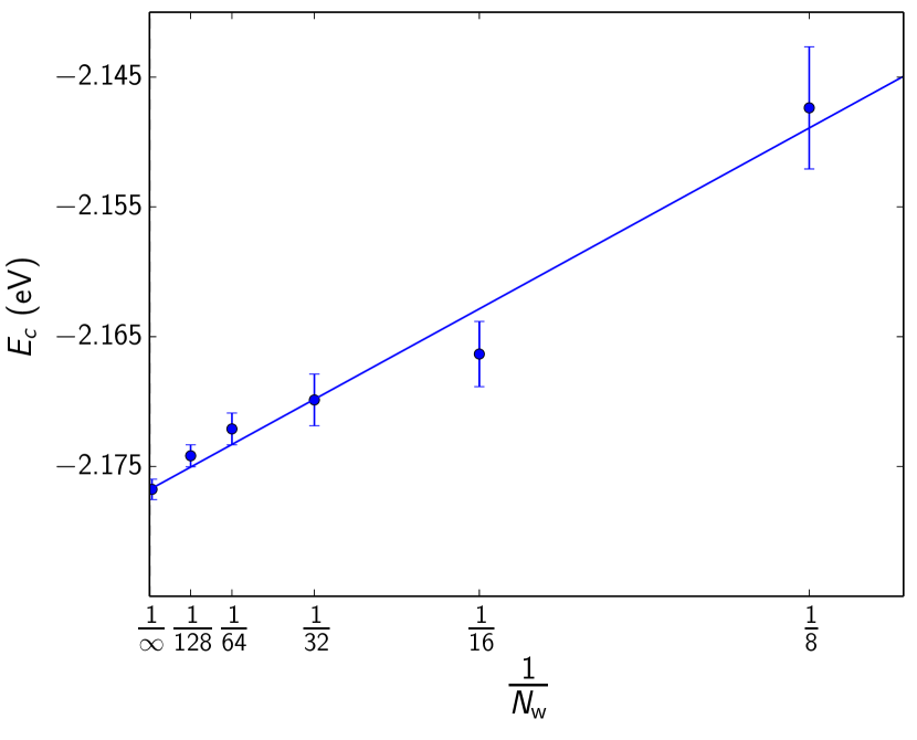
Figure 1: ph-AFQMC correlation energy $E_{\rm c}$ vs. inverse population size for diamond using a $\Gamma$-centered $2\times 2\times 2$ $\mathbf{k}$-point mesh with 8 electrons in 8 HF orbitals per $\mathbf{k}$ point. The population control biases $E_{\rm c}$ when small populations are used. 256 walkers reproduce $E_{\rm c}$ of the infinite population size limit to a precision of 1 meV.

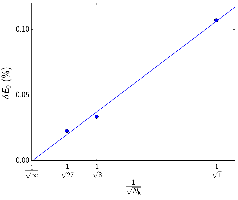
Figure 2: In diamond, the relative error $\delta E_{0}$ of the total energy shows a linear relation with $\frac{1}{\sqrt{N_{\mathbf{k}}}}$ where $N_{\mathbf{k}}$ is the number of $\mathbf{k}$ points. We employed 8 HF orbitals per $\mathbf{k}$ point.

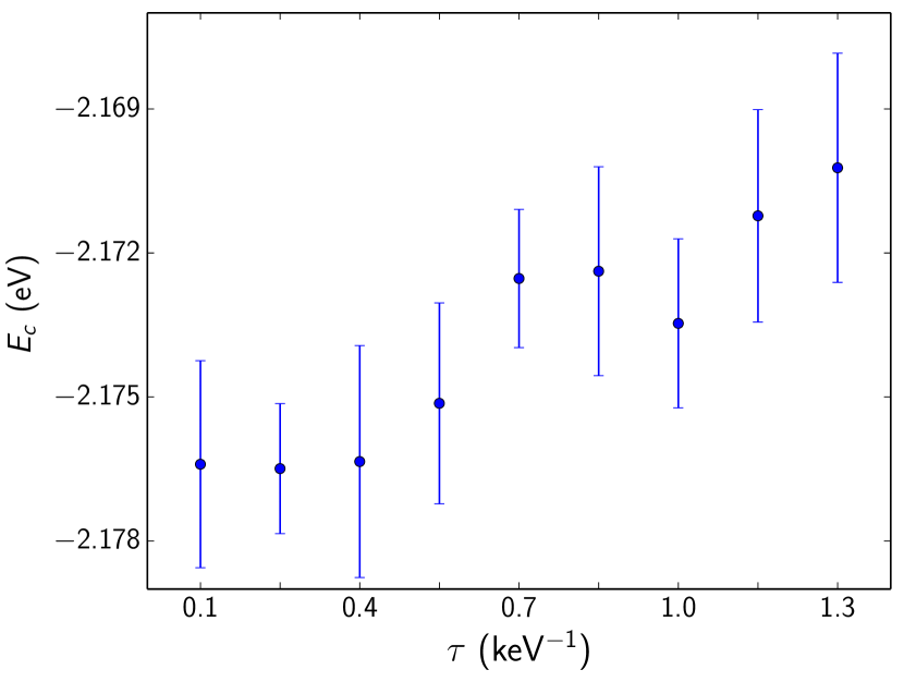
Figure 3: ph-AFQMC correlation energy $E_{\rm c}$ vs. time step $\tau$ for diamond using a $\Gamma$-centered $2\times 2\times 2$ $\mathbf{k}$-point mesh with 8 electrons in 8 HF orbitals per $\mathbf{k}$ point. For all $\tau\leq 0.55$ ${\rm keV}^{-1}$, the calculated $E_{\rm c}$ agree within statistical errors.

We investigate the time-step error and the population-control bias to determine appropriate choices for the time step and the walker population size to ascertain that these systematic errors are smaller than the statistical error.

For small walker populations, the population control biases the correlation energy towards smaller absolute values.Motta and Zhang (2018a) Fig. 1 shows the correlation energy $E_{\rm c}$ of diamond employing a $2\times 2\times 2$ $\mathbf{k}$-point mesh. The error in the correlation energy increases proportionally to the inverse of the population size consistent with what Ref. Motta and Zhang, 2018a reports for molecules. This dependence allows to extrapolate to the infinite population size to correct for this bias.Al-Saidi, Zhang, and Krakauer (2006); Purwanto, Krakauer, and Zhang (2009b) The linear extrapolated value agrees with the result with 2048 walkers. We find that 256 walkers are sufficient to calculate the correlation energy to a precision of 1 meV.

Fig. 2 shows how the relative error $\delta E_{0}$ of the total energy per unit cell scales with number of $\mathbf{k}$ points $N_{\mathbf{k}}$. Here, we defined $\delta E_{0}=\frac{\Delta E_{0}}{E_{0}}$, where $\Delta E_{0}$ is the standard error of the mean. We conclude that utilizing a denser $\mathbf{k}$-point mesh requires a smaller number of MC steps because each walker samples more of the Brillouin zone in each MC step. For a fixed number of walkers, we observe a linear relationship between the relative error and $\frac{1}{\sqrt{N_{\mathbf{k}}}}$. Therefore, denser $\mathbf{k}$-point meshes achieve the same relative error $\delta E_{0}$ in $\frac{1}{\sqrt{N_{\mathbf{k}}}}$ fewer MC steps, if the number of walkers is kept fixed. This observation is very beneficial, and suggests that the statistical errors at different $\mathbf{k}$ points are largely uncorrelated and thus average out. It also means that we can either decrease the number of walkers or the sampling period by $N_{\mathbf{k}}$, when the number of $\mathbf{k}$ points increases.

ph-AFQMC is only accurate up to linear order in the time step $\tau$. The Hubbard-Stratonovich transformation, the Trotter factorizationTrotter (1959), and evaluating the matrix exponential introduce time-step errors.Motta and Zhang (2018a) Fig. 3 illustrates that time steps $\tau\leq 0.55$ ${\rm keV}^{-1}$ yield equivalent correlation energies considering the statistical fluctuations. Larger time steps systematically decrease the absolute value of the correlation energy. In this work, we set the time step to $\tau=0.25$ keV^-1 and expect a negligible (less than statistical error) time-step error without extrapolation.

III.2 Supercell vs. primitive-cell calculation

Table 4: ph-AFQMC correlation energies of the primitive cell ($E^{\rm AF}_{\rm prim}$) and of the corresponding supercell ($E^{\rm AF}_{\rm sc}$) agree within statistical fluctuations. The absolute value of ph-AFQMC correlation-energy is systematically larger than the one obtained with CCSD(T) ($E_{\rm sc}^{\rm CC}$).

crystal		$E^{\rm AF}_{\rm prim}$(eV)	$E^{\rm AF}_{\rm sc}$(eV)	$E^{\rm CC}_{\rm sc}$(eV)
Ne	Fm$\bar{3}$m	$-0.2131(12)$	$-0.2127(12)$	$-0.2107$
C	Fd$\bar{3}$m	$-1.4945(101)$	$-1.4951(54)$	$-1.4830$
BN	F$\bar{4}$3m	$-1.1913(153)$	$-1.1988(52)$	$-1.1861$
LiF	Fm$\bar{3}$m	$-0.5257(18)$	$-0.5223(37)$	$-0.5134$
SiC	F$\bar{4}$3m	$-1.0323(76)$	$-1.0310(70)$	$-1.0252$

In this subsection, we validate our ph-AFQMC implementation with a $\mathbf{k}$-point mesh in the primitive cell against the corresponding supercell. Sampling the Brillouin zone with a $2\times 2\times 2$ $\mathbf{k}$-point mesh is equivalent to a $\Gamma$-point calculation of a supercell enlarged by a factor of two along each axis. The primitive-cell calculation takes advantage of translational symmetry. Therefore, the number of numerical operations is roughly a factor $N_{\mathbf{k}}$ smaller in the primitive cell than in the corresponding supercell. We note in passing that these savings are not always observed in actual calculations, since the matrix dimensions are significantly smaller in the primitive cell, resulting in some performance loss.

For a direct comparison, it is important that the primitive cell and the supercell use the same orbitals. The orbitals are ordered by their eigenvalues $\varepsilon_{n\mathbf{k}}$ at each $\mathbf{k}$ point. In the primitive cell, $\varepsilon_{n+1\mathbf{k}}<\varepsilon_{n\mathbf{k}^{\prime}}$ is possible; whereas in the supercell the former would be included before the latter. To address this, we include more bands in the primitive cell such that all eigenvalues of the supercell are reproduced. Then, we zero all contributions in the primitive cell corresponding to orbitals not present in the supercell.

In Table 4, we verify that our ph-AFQMC implementation computes correlation energies consistent within statistical fluctuations for five different crystals. For all systems, we used 8 HF orbitals per $\mathbf{k}$ point in the primitive cell. Compared to ph-AFQMC, CCSD(T) yields systematically about 10 meV more positive correlation energies, a point we will return to in Section III.4.

III.3 Equation of state

Figure 4: Equation of state for diamond: MP2 (blue) and CCSD (green) yield larger energies than CCSD(T) (red) and ph-AFQMC (black). The optimized lattice constants (dashed vertical lines) are very similar except for the MP2 method. CCSD and ph-AFQMC vertical lines, marking the equilibrium lattice constants, are visually indistinguishable.

In this section, we benchmark the accuracy of the ph-AFQMC total energies against popular deterministic quantum-chemistry methods for diamond, concentrating in particular on relative energies, such as those produced by changes of the volume. Fig. 4 shows the equation of state of diamond for a range of lattice constants. The calculations use a $\Gamma$-centered $3\times 3\times 3$ $\mathbf{k}$-point mesh with 8 HF orbitals per $\mathbf{k}$ point. Compared to ph-AFQMC, the total energies of MP2 and CCSD are 273 meV and 99 meV higher, respectively. In contrast, the CCSD(T) energies are less than 10 meV higher than the ph-AFQMC energies. Furthermore, the optimized lattice constant is 3.578 Å in MP2 considerably smaller than the one of 3.596 Å in ph-AFQMC. CCSD and CCSD(T) yield lattice constants of 3.596 Å and 3.597 Å, respectively, almost identical to the ph-AFQMC result.

III.4 Comparison with coupled-cluster methods for total energies

Figure 5: Relative correlation energies obtained from CCSD (green), ph-AFQMC (black) and ph*-AFQMC (yellow) with respect to the CCSD(T) values for a range of crystals employing a $\Gamma$-centered $2\times 2\times 2$ $\mathbf{k}$-point mesh. The reference values are the CCSD(T) correlation energies, i.e., $\Delta E=E_{\rm c}-E_{\rm c}^{\rm CCSD(T)}$.

This subsection illustrates what accuracy of the correlation energy one can expect from ph-AFQMC compared to coupled-cluster methods. We compute correlation energies for several prototypical semiconductors and insulators with experimental band gaps ranging from 1.4 eV (Si) to 21.7 eV (Ne) to cover different bonding situations. A $\Gamma$-centered $2\times 2\times 2$ $\mathbf{k}$-point mesh allows for a reasonable run time for all systems. For LiF and LiCl, we use 10 electrons and 9 HF orbitals per $\mathbf{k}$ point. All other materials are calculated with 8 valence electrons and 8 HF orbitals per $\mathbf{k}$ point.

We compare the correlation energy of the different methods in Fig. 5. With the exception of the noble-gas crystals, CCSD underestimates the absolute value of the correlation energy by 40 meV to 95 meV compared to ph-AFQMC. In contrast, ph-AFQMC and CCSD(T) agree within 25 meV for the correlation energy of all materials, which is within chemical accuracy.

Sukurma et al.Sukurma et al. (2023) recently proposed a modified version of the phaseless approximation (ph*-AFQMC) to suppress the over-correlation issues of ph-AFQMC. In this approach, the complex nature of the walker weights is retained and if $|\theta_{k}^{w}|\geq\frac{\pi}{2}$ the walker is explicitly killed. Furthermore, the real part of the importance weight instead of the absolute value is used in the update procedure. For more detailed description of ph*-AFQMC we refer the reader to Ref. Sukurma et al., 2023. Fig. 5 demonstrates that ph*-AFQMC yields either consistent or slightly less negative correlation energies compared to the original ph-AFQMC method for the explored solids with the exception of LiF. This is consistent with what Ref. Sukurma et al., 2023 reports for the HEAT set molecules.

Generally, compared to CCSD(T), ph-AFQMC yields more negative correlation energies with the exception of silicon. As to why the ph-AFQMC values are more negative than the CCSD(T) values, we need to speculate. Generally, for weakly correlated systems, coupled-cluster methods converge from above to the exact correlation energy.Bomble et al. (2005) In other words, CCSD(T) has a slight tendency to under-correlate compared to coupled-cluster methods that include triple, quadruple and pentuple excitation operators.Bomble et al. (2005) However, likewise ph-AFQMC can also yield too negative correlation energies.Sukurma et al. (2023) Only if strong double excitations are relevant, ph-AFQMC generally tends to under-correlate. Since both methods are non-variational, it is hard to tell which value is more accurate. The under-correlation for Si and the relatively small single particle band gap of Si, however, suggests that the slight under-correlation for Si is related to ph-AFQMC underestimating energy contributions from double excitations.

Since the ph*-AFQMC correlation energies are also more negative than the CCSD(T) ones, we tend to believe that the ph*-AFQMC are closer to the ground truth. Anyhow, to resolve this issue, obviously more accurate reference methods are required. Booth et al.Booth et al. (2013) employed FCIQMC with the initiator approximation ($i$-FCIQMC) on the same set of materials to investigate the accuracy of standard quantum-chemistry methods. However, recent work suggests that various approximations such as the number of initiators used in this seminal work could have led to an underestimation of the correlation energies.Ghanem, Lozovoi, and Alavi (2019) Underestimated absolute correlation energies were also found for benzene, where $i$-FCIQMC results were 1.5 kcal/mol above the most accurate total energy estimates.Eriksen et al. (2020); Blunt, Thom, and Scott (2019) Hence, although our results are within chemical accuracy of the reference values, fully converged CI calculations with consistent basis sets and pseudopotentials are required to resolve this ambiguity. In this context it is also worth noting that Lee et al.Lee, Malone, and Morales (2019) carried out a comparative study using ph-AFQMC for the uniform electron gas. Their findings show that ph-AFQMC correlation energies are in good agreement with $i$-FCIQMC at densities corresponding to $r_{S}=1.0$ and $r_{S}=2.0$, whereas at $r_{S}=5.0$ the $i$-FCIQMC correlation are more negative than those obtained with ph-AFQMC.Lee, Malone, and Morales (2019); Shepherd, Booth, and Alavi (2012) CCSDT theory yields energies in good agreement with $i$-FCIQMC at high densities but underestimates the absolute correlation energies at densities corresponding $r_{S}=2.0$ and $r_{S}=5.0$.Lee, Malone, and Morales (2019); Neufeld and Thom (2017) Although CCSD(T) and CCSDT can differ, this is not expected for the investigated relatively small system sizes with about 14 electrons. Therefore, the uniform electron gas findings also support our hypothesis that ph*-AFQMC is closer to the ground truth for the investigated solids in this work.

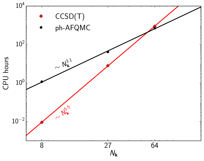
Figure 6: System size scaling of ph-AFQMC (black) and CCSD(T) (red) for various $\Gamma$-centered $\mathbf{k}$-point meshes of diamond. We employed 8 HF orbitals per $\mathbf{k}$ point. Both ph-AFQMC and CCSD(T) calculations were performed on a single-socket AMD EPYC 7713 and one MPI process.

ph-AFQMC exhibits a better scaling with system size compared to CCSD(T). To illustrate this, we benchmark the scaling of our ph-AFQMC Python code against the VASP CCSD(T) code developed in Fortran. In Fig. 6, we explore the scaling for various regular $\Gamma$-centered $\mathbf{k}$-point meshes of diamond with 8 orbitals per $\mathbf{k}$ point. The CCSD(T) computational cost is slightly larger than for ph-AFQMC at $N_{\mathbf{k}}=64$, which is the largest system size we have investigated in this work. Empirically, ph-AFQMC shows a roughly-cubic scaling with $N_{\mathbf{k}}$ while CCSD(T) approximately scales as $N_{\mathbf{k}}^{5.5}$, here.

III.5 Down-sampling of the correlation energy

Figure 7: Diamond correlation energy $E_{\rm c}$ sampled with an $n_{\mathbf{k}}\times n_{\mathbf{k}}\times n_{\mathbf{k}}$ $\mathbf{k}$-point mesh. The solid lines extrapolate to $n_{\mathbf{k}}\rightarrow\infty$ using $n_{\mathbf{k}}=3$ and $n_{\mathbf{k}}=4$. (a) Comparison of the down-sampled correlation energy (blue) with the one obtained with the complete basis set for MP2 (orange). The extrapolated lines are visually indistinguishable. (b) The down-sampled correlation energies for MP2 (blue), CCSD (green), CCSD(T) (red) and ph-AFQMC (black).

The preceding subsections illustrated benchmark calculations for the PAW method with coarse $\mathbf{k}$-point meshes and few HF orbitals. In this subsection, we present a strategy to perform predictive ph-AFQMC calculations. This strategy is outlined and tested for diamond. We test two commonly used techniques to converge to the complete basis-set (CBS) limit. First, natural orbitals Löwdin (1955); Bender and Davidson (1966); Davidson (1972); Thunemann et al. (1977) reduce the number of virtual orbitals required to converge to the correlation energy. We use natural orbitals obtained by the random phase approximation.Ramberger et al. (2019); Humer et al. (2022) Second, because differences converge faster than absolute energies, down-sampling via energy differencesGrüneis et al. (2011) allows to estimate the CBS correlation energy at significantly reduced cost.

Specifically, we intend to extrapolate the correlation energy to infinitely-dense $\mathbf{k}$-point meshes. Here, we use $n_{\mathbf{k}}\times n_{\mathbf{k}}\times n_{\mathbf{k}}$ $\mathbf{k}$-point meshes for a linear fit to zero volume per $\mathbf{k}$ point based on $n_{\mathbf{k}}=3$ and $n_{\mathbf{k}}=4$. To obtain the down-sampled correlation energy at a denser $\mathbf{k}$-point mesh, we compute the energy difference when increasing $n_{\mathbf{k}}$ at fixed number of orbitals per $\mathbf{k}$ point ${n}_{\rm b}$

$$\Delta_{\rm c}(n_{\mathbf{k}},{n}_{\rm b})=E_{\rm c}(n_{\mathbf{k}}+1,{n}_{\rm b})-E_{\rm c}(n_{\mathbf{k}},{n}_{\rm b})~{}.$$ (24)

We converge the correlation energy at the coarser $\mathbf{k}$-point mesh with respect to the number of orbitals per $\mathbf{k}$ point ${n}_{\rm b}$. Adding the difference yields an approximation for the correlation energy at the dense mesh

$$E_{\rm c}(n_{\mathbf{k}}+1)\approx\tilde{E}_{\rm c}(n_{\mathbf{k}}+1,{n}_{\rm b})=E_{\rm c}(n_{\mathbf{k}})+\Delta_{\rm c}(n_{\mathbf{k}},{n}_{\rm b}).$$ (25)

One can then iterate this procedure with a reduced ${n}_{\rm b}$ to obtain approximations for even denser meshes.

To verify this procedure, we evaluate the correlation energy of MP2 with the down-sampling technique

$$\begin{split}E_{\rm c}(n_{\mathbf{k}}=3)&\approx E_{\rm c}(n_{\mathbf{k}}=2)+\Delta_{\rm c}(n_{\mathbf{k}}=2,{n}_{\rm b}=16),\\ E_{\rm c}(n_{\mathbf{k}}=4)&\approx E_{\rm c}(n_{\mathbf{k}}=3)+\Delta_{\rm c}(n_{\mathbf{k}}=3,{n}_{\rm b}=8)~{}.\end{split}$$ (26)

We compute the correlation energy $E_{\rm c}(n_{\mathbf{k}}=2)$ with 64 natural orbitals. Fig. 7a compares these energies to the CBS where all calculations use ${n}_{\rm b}=64$; the two sets of data points are visually indistinguishable. Extrapolating to the infinitely dense $\mathbf{k}$-point mesh yields a correlation energy of $-$8.987 eV for the CBS and of $-$8.986 eV for the down-sampled energies.

We employ the down-sampling technique for the correlation energy of MP2, CCSD, CCSD(T), and ph-AFQMC. Fig. 7b shows the resulting extrapolations. For MP2, the extrapolation from $n_{\mathbf{k}}=3$ to $n_{\mathbf{k}}=4$ shows a different slope and a large deviation for $n_{\mathbf{k}}=2$ compared to the other methods. In contrast, the ph-AFQMC correlation energy would only change by 9 meV if one used $n_{\mathbf{k}}=2$ and $n_{\mathbf{k}}=3$ for the extrapolation. CCSD(T) and ph-AFQMC agree within statistical errors for denser meshes. The extrapolated correlation energy is $-$9.116 eV for CCSD(T) and $-$9.106(30) eV for ph-AFQMC.

Table 5: CCSD(T) and ph-AFQMC down-sampled correlation energies of the primitive cell for various $n_{\mathbf{k}}$ and $n_{\rm b}$.

$n_{\mathbf{k}}$	$n_{\rm b}$	$E_{\rm c}^{\rm CC}$ (eV)	$E_{\rm c}^{\rm AF}$ (eV)
2	64	-8.661	-8.693(10)
3	16	-8.966	-8.977(13)
4	8	-9.052	-9.052(16)

There are two important conclusions we can draw from this test, and these are also more clearly borne out in Table 5. First, the difference in the correlation energy between ph-AFQMC and CCSD(T) does not increase as the number of virtual orbitals increases. On the contrast it seems to decrease, although we might need better statistical accuracy and tests for more materials to be certain. This observation is fully in line with the observations we recently made for small molecules.Sukurma et al. (2023) This also means that the potential errors of both methods relate to low energy excitations, and tests using few states are already very meaningful. Second, increasing the number of ${\mathbf{k}}$ points does not change the difference between ph-AFQMC and CCSD(T) appreciably (note that our error bars for the densest ${\mathbf{k}}$-point mesh are fairly sizable). Hence, the excellent agreement of CCSD(T) and ph-AFQMC prevails even in the thermodynamic limit.

IV Conclusion

ph-AFQMC is potentially a great method to obtain very accurate reference results for solid-state systems. The present work merely tries to establish that ph-AFQMC is competitive to CCSD(T) and is capable to yield very accurate results for solids with quite different characteristics. As already emphasized in the introduction, one advantage of ph-AFQMC is that it is fully compatible with other quantum-chemistry methods, such as MP2, CCSD or CCSD(T). This means that one can directly compare predicted energies with these and other well-established quantum-chemistry methods. It is clear and well understood that this also entails significant disadvantages, such as a slow convergence with respect to the number of virtual states (unoccupied orbitals) included in the calculations. Certainly DMC is superior in this respect, but validation of DMC against other quantum-chemistry methods is notoriously difficult. For instance, recent conflicting results for localized coupled-cluster and DMC calculations for large weakly bonded molecules are very difficult to disentangle, as absolute energies can not be compared between the methods. Al-Hamdani et al. (2021)

We have demonstrated that in the thermodynamic limit—that is for many $\mathbf{k}$ points and virtual bands—ph-AFQMC is superior to a quite efficient Fortran implementation of CCSD(T). This is insofar remarkable, as our own implementation is not yet fully optimized and uses Python. Specifically, CCSD(T) possesses a disadvantageous scaling with both the number of $\mathbf{k}$ points and the number of virtual orbitals. In practice we found that our ph-AFQMC code scales quadratic with respect to the number of unoccupied orbitals, and cubic with respect to the number of $\mathbf{k}$ points. This means it will always outpace a CCSD(T) code for sufficiently large systems.

The second important observation is that for the solids investigated here, CCSD(T) and ph-AFQMC agree within chemical accuracy for absolute energies. Although we have done the comparison initially for few $\mathbf{k}$ points and few bands, our tests for diamond clearly show that the differences will not increase as the number of $\mathbf{k}$ points or bands increases. The excellent agreement also means that one can potentially mix and match ph-AFQMC and CCSD(T) in actual investigations and rely on advantages of one or the other method for specific sub-problems.

Last but not least, we have made one somewhat disconcerting observation: our ph-AFQMC correlation energies are generally slightly more negative than the corresponding CCSD(T) energies (but again well within chemical accuracy). It is well understood that CCSD(T) often converges from above, so potentially better agreement would be obtained when quadruple and pentuple excitation operators are included in the coupled-cluster calculations. However, ph-AFQMC—being non-variational—also sometimes over-correlates; so maybe the CCSD(T) values are more accurate after all. The available data are clearly not sufficient to draw a final conclusion. Specifically, the reported FCIQMC values hint towards even smaller absolute correlation energies than CCSD(T). This we believe to be unlikely: for instance for small molecules, CCSD(T) certainly underestimates the correlation energy consistently.Bomble et al. (2005); Sukurma et al. (2023) Why should this be any different for simple prototypical insulators and semiconductors? So reference-type calculations for solids using few $\mathbf{k}$ points and bands would be very helpful to solve this small but important "riddle".

Author declarations

Conflict of Interest

The authors have no conflicts to disclose.

Author Contributions

Amir Taheridehkordi: Investigation, Methodology, Software, Writing – original draft. Martin Schlipf: Software, Writing – review & editing. Zoran Sukurma: Methodology, Writing – review & editing. Moritz Humer: Writing – review & editing. Andreas Grüneis: Writing – review & editing. Georg Kresse: Project administration, Writing – review & editing.

Data availability

The data that support the findings of this study are available within the article. The Python code is available from the first author upon reasonable request.

Appendix A Hamiltonian

Units used in the appendix and throughout the manuscript are Hatree-units. The electronic Born-Oppenheimer Hamiltonian consists of one-body and two-body parts Born and Oppenheimer (1927); Szabo and Ostlund (2012)

$$\hat{H}=\hat{H}_{1}+\hat{H}_{2}.$$ (27)

The one-body part is defined as

$$\hat{H}_{1}=\sum_{pq}t_{pq}\hat{a}_{p}^{\dagger}\hat{a}_{q},$$ (28)

where $\hat{a}_{p}$ ($\hat{a}^{\dagger}_{p}$) are fermionic annihilation (creation) operators associated with an orthonormal basis $\phi_{p}$. The matrix elements are

$$t_{pq}=\int{\rm d}\mathbf{r}\phi_{p}^{*}(\mathbf{r})\bigg{(}-\frac{1}{2}\hat{\nabla}^{2}-\sum_{a}\frac{Z_{a}}{|\mathbf{r}-\mathbf{R}_{a}|}\bigg{)}\phi_{q}(\mathbf{r}),$$ (29)

where $\mathbf{R}_{a}$ and $Z_{a}$ denote the position and atomic number of the nuclei with label $a$, respectively. The two-body part of the Hamiltonian (27) describes the electron-electron interaction

$$\hat{H}_{2}=\frac{1}{2}\sum_{pqrs}\langle pq|rs\rangle\hat{a}_{p}^{\dagger}\hat{a}_{q}^{\dagger}\hat{a}_{s}\hat{a}_{r}$$ (30)

introducing an abbreviation for the Coulomb integral

$$\langle pq|rs\rangle=\int{\rm d}\mathbf{r}{\rm d}\mathbf{r}^{\prime}\phi_{p}^{*}(\mathbf{r})\phi_{q}^{*}(\mathbf{r}^{\prime})\frac{1}{|\mathbf{r}-\mathbf{r}^{\prime}|}\phi_{r}(\mathbf{r})\phi_{s}(\mathbf{r}^{\prime}).$$ (31)

Next, we introduce a $\mathbf{k}$-point mesh to sample the Brillouin zone. The one-body part is diagonal in the Bloch vector $\mathbf{k}$

$$\hat{H}_{1}=\sum_{\mathbf{k}}\sum_{pq}t_{pq}(\mathbf{k})\hat{a}_{p\mathbf{k}}^{\dagger}\hat{a}_{q\mathbf{k}}.$$ (32)

The two-body part has to fulfill momentum conservation Motta, Zhang, and Chan (2019)

$$\hat{H}_{2}=\frac{1}{2}\sum_{\mathbf{k}_{p}+\mathbf{k}_{q}=\mathbf{k}_{r}+\mathbf{k}_{s}}\sum_{prqs}\langle p\mathbf{k}_{p},q\mathbf{k}_{q}|r\mathbf{k}_{r},s\mathbf{k}_{s}\rangle\\ \times\hat{a}_{p\mathbf{k}_{p}}^{\dagger}\hat{a}_{q\mathbf{k}_{q}}^{\dagger}\hat{a}_{s\mathbf{k}_{s}}\hat{a}_{r\mathbf{k}_{r}},$$ (33)

which we rewrite introducing the transferred momentum $\mathbf{q}=\mathbf{k}_{p}-\mathbf{k}_{r}$

$$\hat{H}_{2}=\frac{1}{2}\sum_{\mathbf{q}\mathbf{k}_{r}\mathbf{k}_{s}}\sum_{prqs}\langle p\mathbf{k}_{r}+\mathbf{q},q\mathbf{k}_{s}-\mathbf{q}|r\mathbf{k}_{r},s\mathbf{k}_{s}\rangle\\ \times\hat{a}_{p\mathbf{k}_{r}+\mathbf{q}}^{\dagger}\hat{a}_{q\mathbf{k}_{s}-\mathbf{q}}^{\dagger}\hat{a}_{s\mathbf{k}_{s}}\hat{a}_{r\mathbf{k}_{r}}.$$ (34)

Using a plane-wave basis set, we express electron-repulsion integrals in the reciprocal space as

$$\langle p\mathbf{k}_{r}+\mathbf{q},q\mathbf{k}_{s}-\mathbf{q}|r\mathbf{k}_{r},s\mathbf{k}_{s}\rangle=\sum_{\mathbf{G}}\frac{4\pi}{|\mathbf{G}-\mathbf{q}|^{2}}\\ \times\rho_{pr\mathbf{k}_{r}}(\mathbf{q},\mathbf{G})\rho^{\ast}_{sq\mathbf{k}_{s}-\mathbf{q}}(\mathbf{q},\mathbf{G}).$$ (35)

Here, we introduced the two-orbital density $\rho$

$$\rho_{pr\mathbf{k}_{r}}(\mathbf{q},\mathbf{G})=\frac{1}{\sqrt{\Omega}}\int{\rm d}\mathbf{r}{\rm{e}}^{i(\mathbf{G}-\mathbf{q})\cdot\mathbf{r}}\phi_{p\mathbf{k}_{r}+\mathbf{q}}^{\ast}(\mathbf{r})\phi_{r\mathbf{k}_{r}}(\mathbf{r})$$ (36)

and $\Omega$ is the volume of the system. The summation over plane waves in Eq. (35) is truncated by an energy cutoff $G^{2}/2=E_{\rm{cut}}$.

Finally, we commute $\hat{a}_{r\mathbf{k}_{r}}$ to the left in Eq. (34) using the anti-commutation relations between the fermionic operators $\{\hat{a}_{r}^{\dagger},\hat{a}_{p}\}=\hat{a}_{r}^{\dagger}\hat{a}_{p}+\hat{a}_{p}\hat{a}_{r}^{\dagger}=\delta_{rp}$. This yields the modified one- and two-body operators shown in Eqs. (2) and (3), respectively. The updated one-body matrix elements are

$$h_{pq}(\mathbf{k})=t_{pq}(\mathbf{k})-\frac{1}{2}\sum_{\mathbf{k}_{r}}\sum_{r}\langle p\mathbf{k},r\mathbf{k}_{r}|r\mathbf{k}_{r},q\mathbf{k}\rangle.$$ (37)

We introduce the operators

$$\hat{L}^{\prime}_{\mathbf{qG}}=\frac{\sqrt{4\pi}}{|\mathbf{G}-\mathbf{q}|}\sum_{\mathbf{k}_{r}}\sum_{pr}\rho_{pr\mathbf{k}_{r}}(\mathbf{q},\mathbf{G})\hat{a}_{p\mathbf{k}_{r}+\mathbf{q}}^{\dagger}\hat{a}_{r\mathbf{k}_{r}}$$ (38)

to write the two-body operator in terms of one-body operators:

$$\hat{H}_{2}^{\prime}=\frac{1}{2}\sum_{\mathbf{q}\mathbf{G}}\hat{L}^{\prime}_{\mathbf{qG}}\hat{L}^{\prime\dagger}_{\mathbf{qG}}.$$ (39)

Appendix B VASP interface

For the ph-AFQMC code, we require the one-body matrix $t_{pq}(\mathbf{k})$ in Eq. (32) and the two-body tensor

$$L^{\prime}_{pr\mathbf{k}_{r}\mathbf{q}\mathbf{G}}=\frac{\sqrt{4\pi}}{|\mathbf{G}-\mathbf{q}|}\rho_{pr\mathbf{k}_{r}}(\mathbf{q},\mathbf{G}),$$ (40)

in Eq. (38). We compute these using VASP.Blöchl (1994); Kresse and Joubert (1999) Typically, we use a smaller energy cutoff for the two-body tensor than for the one-body matrix; this can lead to small inconsistencies in the energy of the HF ground state. To address this, we pre-calculate the fully self-consistent one-body HF-Hamiltonian matrix $t_{pq}^{\mathrm{H}F}(\mathbf{k})$ within the VASP code. This term includes the kinetic energy, the ion-electron potential, the Hartree potential and the Fock exchange operator. Details on the VASP implementation are given in Ref. Paier et al., 2005. For the canonical HF orbitals, the matrix is diagonal and equal to the eigenvalues $t_{pq}^{\mathrm{H}F}(\mathbf{k})=\varepsilon_{p\mathbf{k}}\delta_{pq}$. For the ph-AFQMC calculation, we require only the kinetic energy term and the ion-electron potential. We compute this term by subtracting the Hartree ($J_{pq}(\mathbf{k})$) and Fock contribution ($K_{pq}(\mathbf{k})$) calculated from the two-body tensors (with the lower energy cutoff, which is equal to the plane-wave energy cutoff) and subtract them to obtain the matrix elements

$$t_{pq}(\mathbf{k})=t_{pq}^{\mathrm{H}F}(\mathbf{k})-J_{pq}(\mathbf{k})+K_{pq}(\mathbf{k}),$$ (41)

with

$$\begin{split}&J_{pq}(\mathbf{k})=2\sum_{i\mathbf{k}^{\prime}\mathbf{G}}\bigg{(}\sum_{\mathbf{q}}L^{\prime}_{\mathbf{qG}}\bigg{)}_{p\mathbf{k},q\mathbf{k}}\bigg{(}\sum_{\mathbf{q}}L^{\prime}_{\mathbf{qG}}\bigg{)}^{*}_{i\mathbf{k}^{\prime},i\mathbf{k}^{\prime}},\\ &K_{pq}(\mathbf{k})=\sum_{i\mathbf{k}^{\prime}\mathbf{G}}\bigg{(}\sum_{\mathbf{q}}L^{\prime}_{\mathbf{qG}}\bigg{)}_{p\mathbf{k},i\mathbf{k}^{\prime}}\bigg{(}\sum_{\mathbf{q}}L^{\prime}_{\mathbf{qG}}\bigg{)}^{*}_{q\mathbf{k},i\mathbf{k}^{\prime}}.\end{split}$$ (42)

where index $i$ goes over the occupied states. This strategy minimized truncation errors that would occur if we just exported the kinetic energy and the electron-ion matrix elements from the VASP code. For instance, a self-consistent HF calculation using the one-body Hamiltonian $t_{pq}(\mathbf{k})$ and the two body tensors $L^{\prime}_{\mathbf{qG}}$ yields exactly the same eigenvalues as the preceding VASP calculation.

For the two-orbital tensor defined above, we loop $\mathbf{q}$ and $\mathbf{k}_{p}$ over the mesh sampling the Brillouin zone. Each pair corresponds to a $\mathbf{k}_{r}=\mathbf{k}_{p}-\mathbf{q}$ conserving the momentum. $\mathbf{k}_{r}$ may lay outside of the first Brillouin zone; folding it back with a reciprocal lattice vector $\delta\mathbf{G}$ introduces a phase $\varphi=\exp[i\,\delta\mathbf{G}\cdot\mathbf{r}]$. The orbitals $\phi_{r\mathbf{k}_{r}}$ consist of a smooth pseudo-orbital $\tilde{\phi}_{r\mathbf{k}_{r}}$ augmented by the difference of atomic orbitals $\phi^{1}_{\nu}$ and their pseudized counterpart $\tilde{\phi}^{1}_{\nu}$. Projectors $p_{\nu}^{1}$ determine the replaced fraction of the pseudo-orbital

$$|\phi_{r\mathbf{k}_{r}}\rangle=|\tilde{\phi}_{r\mathbf{k}_{r}}\rangle+\sum_{\nu}\bigl{(}|\phi_{\nu}^{1}\rangle-|\tilde{\phi}_{\nu}^{1}\rangle\bigr{)}\langle p_{\nu}^{1}|\tilde{\phi}_{r\mathbf{k}_{r}}\rangle.$$ (43)

The superscript 1 indicates one-center quantities that are only nonzero within the PAW sphere of one atom. Non-local operators contain coupling between the pseudo-orbital and the one-center terms.Blöchl (1994) Therefore the two-orbital density given by Eq. (36) consists of a pseudo and a one-center contribution

$$\rho_{pr\mathbf{k}_{r}}(\mathbf{q},\mathbf{G})=\tilde{\rho}_{pr\mathbf{k}_{r}}(\mathbf{q},\mathbf{G})+\rho_{pr\mathbf{k}_{r}}^{1}(\mathbf{q},\mathbf{G}).$$ (44)

Representing the one-center term would require a very dense real-space grid. To avoid this one introduces a compensation density $\hat{\rho}$ that restores the multi-poles of the all-electron density on the plane-wave grid.Kresse and Joubert (1999); Paier et al. (2005) As a result, the one-center density has no Coulomb interaction outside the PAW sphere. We also neglect the contributions inside the PAW sphere in the present work:

$$\rho_{pr\mathbf{k}_{r}}(\mathbf{q},\mathbf{G})\approx\tilde{\rho}_{pr\mathbf{k}_{r}}(\mathbf{q},\mathbf{G})+\hat{\rho}_{pr\mathbf{k}_{r}}(\mathbf{q},\mathbf{G}).$$ (45)

To make up for the neglect of the terms in the PAW spheres, we use shape restoration. Shape restorations allows to accurately restore the all-electron density distribution inside the PAW spheres even on a coarse plane-wave grid.Shishkin and Kresse (2006); Unzog, Tal, and Kresse (2022) It is routinely used in VASP for calculations using, e.g., the random phase approximation and sufficiently accurate to obtain highly reliable correlation energy differences.Humer et al. (2022) Here, we set LMAXFOCKAE = 4 to force an accurate treatment for the charge augmentation up to the angular quantum number of 4. Finally, we combine the two-orbital density with the square of the Coulomb potential and correct the phase $\varphi$ if necessary.

The one-body matrix $t_{pq}(\mathbf{k})$ and the two-body tensor $L^{\prime}_{pr\mathbf{k}_{r}\mathbf{q}\mathbf{G}}$ are each exported in NPY format to facilitate easy processing in Python.

Appendix C Time evolution

To determine the ground-state wavefunction $|\Phi_{0}\rangle$ of a system governed by a Hamiltonian $\hat{H}$, the imaginary-time propagator is applied to the initial wavefunction $|\Psi_{\rm I}\rangle$ in the infinite time limit Zhang and Krakauer (2003)

$$|\Phi_{0}\rangle\propto\lim_{\beta\to\infty}e^{-\beta\hat{H}}|\Psi_{\rm I}\rangle.$$ (46)

In practice, one approaches the ground-state wavefunction by repeated application of the imaginary-time propagator for a small time step $\tau=\frac{\beta}{n}$

$$\lim_{\beta\to\infty}e^{-\beta\hat{H}}|\Psi_{\rm I}\rangle=\lim_{n\to\infty}\bigg{[}{\rm e}^{-\tau\hat{H}}\bigg{]}^{n}|\Psi_{\rm I}\rangle.$$ (47)

The Hubbard-Stratonovich transformationStratonovich (1957); Hubbard (1959) translates the two-body part to an integral of one-body operators

$${\rm e}^{-\tau\hat{H}}=\int{\rm d}\mathbf{x}p(\mathbf{x})\hat{B}(\mathbf{x})+O(\tau^{2}).$$ (48)

$p(\mathbf{x})$ is the normal distribution function

$$p(\mathbf{x})=(2\pi)^{-N_{g}/2}{\rm e}^{-\frac{1}{2}|\mathbf{x}|^{2}},$$ (49)

where $N_{g}$ is the number of components of $\mathbf{x}$. The propagation operator $\hat{B}$ is defined in Eq. (15) in the main text.

Appendix D Force bias

The force bias is given by

$$f_{\mathbf{q}g,k}^{w}=-i\sqrt{\tau}\frac{\langle\Psi_{\rm T}|\hat{\mathfrak{L}}_{\mathbf{q}g}|\Psi_{k}^{w}\rangle}{\langle\Psi_{\rm T}|\Psi_{k}^{w}\rangle}.$$ (50)

A creation-annihilation operator pair is

$$\frac{\langle\Psi_{\rm T}|\hat{a}_{P}^{\dagger}\hat{a}_{R}|\Psi_{k}^{w}\rangle}{\langle\Psi_{\rm T}|\Psi_{k}^{w}\rangle}=\Bigl{[}\Psi_{k}^{w}\big{(}\Psi_{\rm T}^{\dagger}\Psi_{k}^{w}\big{)}^{-1}\Psi_{\rm T}^{\dagger}\Bigr{]}_{RP}$$ (51)

in matrix representation. $P$ and $R$ are composite indices for band and momentum, i.e., $R\equiv(r\mathbf{k}_{r})$. We compute the biorthogonalized orbitals in every step

$$\Theta_{k}^{w}=\Psi_{k}^{w}\big{(}\Psi_{\rm T}^{\dagger}\Psi_{k}^{w}\big{)}^{-1}.$$ (52)

The action of the $\hat{\mathfrak{L}}$ operator onto the trial wavefunction is precomputed

$$\alpha_{{\mathbf{q}g}}=\Psi_{\rm T}^{\dagger}\mathfrak{L}_{{\mathbf{q}g}}~{}.$$ (53)

We convolute these two matrices to obtain the force bias for a non-spin-polarized system

$$f_{{\mathbf{q}g,k}}^{w}=-2i\sqrt{\tau}{\rm Tr}[\Theta_{k}^{w}\alpha_{\mathbf{q}g}].$$ (54)

Appendix E Local energy

The local energy is

$$E_{\rm{loc}}(\Psi_{k}^{w})=\frac{\langle\Psi_{\rm T}|\hat{H}_{1}+\hat{H}_{2}|\Psi_{k}^{w}\rangle}{\langle\Psi_{\rm T}|\Psi_{k}^{w}\rangle}.$$ (55)

Similar to the force bias we use Eq. (51) to evaluate the one-body part in the matrix representation. For a non-spin-polarized system we obtain

$$\begin{split}E_{1}(\Psi_{k}^{w})=2{\rm{Tr}}[\Psi_{\rm T}^{\dagger}H_{1}\Theta_{k}^{w}].\end{split}$$ (56)

For the two-body part we consider the generalized Wick’s theorem: Wick (1950); Balian and Brezin (1969)

$$\begin{split}\frac{\langle\Psi_{\rm T}|\hat{a}_{P}^{\dagger}\hat{a}_{Q}^{\dagger}\hat{a}_{S}\hat{a}_{R}|\Psi^{w}\rangle}{\langle\Psi_{\rm T}|\Psi^{w}\rangle}=\mathcal{G}_{PR}^{w}\mathcal{G}_{QS}^{w}-\mathcal{G}_{PS}^{w}\mathcal{G}_{QR}^{w}.\end{split}$$ (57)

Here, $\mathcal{G}$ is the Green’s function

$$\mathcal{G}_{PR}^{w}\equiv\mathcal{G}_{PR}(\Psi^{w})=\frac{\langle\Psi_{\rm T}|\hat{a}_{P}^{\dagger}\hat{a}_{R}|\Psi^{w}\rangle}{\langle\Psi_{\rm T}|\Psi^{w}\rangle}$$ (58)

that we know to compute from Eq. (51).

Thus, the two-body part of the local energy is split into Hartree- and exchange-like terms:

$$\begin{split}E_{2}(\Psi_{k}^{w})=E_{\rm H}(\Psi_{k}^{w})+E_{\rm X}(\Psi_{k}^{w}).\end{split}$$ (59)

For a non-spin-polarized system:

$$\begin{split}E_{\rm H}(\Psi_{k}^{w})=2\sum_{\mathbf{q}}\sum_{g=1}^{N_{\mathbf{q}g}}{\rm{Tr}}[\Theta_{k}^{w}\alpha_{{\mathbf{q}}{{g}}}]{\rm{Tr}}[\Theta_{k}^{w}\beta_{{\mathbf{q}}{{g}}}],\\ E_{\rm X}(\Psi_{k}^{w})=-\sum_{\mathbf{q}}\sum_{g=1}^{N_{\mathbf{q}g}}{\rm{Tr}}[(\Theta_{k}^{w}\alpha_{{\mathbf{q}}{{g}}})(\Theta_{k}^{w}\beta_{{\mathbf{q}}{{g}}})],\end{split}$$ (60)

where for each specific $g$ we have

$$\begin{split}&\beta_{{\mathbf{q}}{{g}}}=\Psi_{\rm T}^{\dagger}\mathfrak{L}^{\dagger}_{{\mathbf{q}g}},\end{split}$$ (61)

and $\alpha_{{\mathbf{q}}{\rm{g}}}$ is given by Eq. (53).

References

- Kohn and Sham (1965) W. Kohn and L. J. Sham, Phys. Rev. 140, A1133–A1138 (1965).
- Kohn (1999) W. Kohn, Rev. Mod. Phys. 71, 1253–1266 (1999).
- Blöchl (1994) P. E. Blöchl, Phys. Rev. B 50, 17953 (1994).
- Kresse and Joubert (1999) G. Kresse and D. Joubert, Phys. Rev. B 59, 1758 (1999).
- Paier et al. (2005) J. Paier, R. Hirschl, M. Marsman, and G. Kresse, J. Chem. Phys. 122, 234102 (2005).
- Lejaeghere et al. (2016) K. Lejaeghere, G. Bihlmayer, T. Björkman, P. Blaha, S. Blügel, V. Blum, D. Caliste, I. E. Castelli, S. J. Clark, A. Dal Corso, et al., Science 351, 1394 (2016).
- Humer et al. (2022) M. Humer, M. E. Harding, M. Schlipf, A. Taheridehkordi, Z. Sukurma, W. Klopper, and G. Kresse, J. Chem. Phys. 157, 194113 (2022).
- Burke (2012) K. Burke, J. Chem. Phys. 136, 150901 (2012).
- Curtiss et al. (1997) L. A. Curtiss, K. Raghavachari, P. C. Redfern, and J. A. Pople, J. Chem. Phys. 106, 1063–1079 (1997).
- Paier, Marsman, and Kresse (2007) J. Paier, M. Marsman, and G. Kresse, J. Chem. Phys. 127, 024103 (2007).
- Dobson et al. (2001) J. F. Dobson, K. McLennan, A. Rubio, J. Wang, T. Gould, H. M. Le, and B. P. Dinte, Aust. J. Chem. 54, 513–527 (2001).
- Raghavachari et al. (1989) K. Raghavachari, G. W. Trucks, J. A. Pople, and M. Head-Gordon, Chem. Phys. Lett. 157, 479–483 (1989).
- Bartlett and Musiał (2007) R. J. Bartlett and M. Musiał, Rev. Mod. Phys. 79, 291 (2007).
- Grüneis (2015) A. Grüneis, J. Chem. Phys. 143, 102817 (2015).
- Gruber et al. (2018) T. Gruber, K. Liao, T. Tsatsoulis, F. Hummel, and A. Grüneis, Phys. Rev. X 8, 021043 (2018).
- Szabo and Ostlund (2012) A. Szabo and N. S. Ostlund, Modern quantum chemistry: introduction to advanced electronic structure theory (Courier Corporation, 2012).
- Cramer (2013) C. J. Cramer, Essentials of computational chemistry: theories and models (John Wiley & Sons, 2013).
- Vogiatzis et al. (2017) K. D. Vogiatzis, D. Ma, J. Olsen, L. Gagliardi, and W. A. de Jong, J. Chem. Phys. 147, 184111 (2017).
- Al-Hamdani et al. (2021) Y. S. Al-Hamdani, P. R. Nagy, A. Zen, D. Barton, M. Kállay, J. G. Brandenburg, and A. Tkatchenko, Nat. Commun. 12, 3927 (2021).
- Nagy, Samu, and Kállay (2018) P. R. Nagy, G. Samu, and M. Kállay, J. Chem. Theory Comput. 14, 4193–4215 (2018).
- Nagy and Kállay (2019) P. R. Nagy and M. Kállay, J. Chem. Theory Comput. 15, 5275–5298 (2019).
- Zaleśny et al. (2011) R. Zaleśny, M. G. Papadopoulos, P. G. Mezey, and J. Leszczynski, Linear-Scaling Techniques in Computational Chemistry and Physics: Methods and Applications, Vol. 13 (Springer Science & Business Media, 2011).
- Kalos, Levesque, and Verlet (1974) M. H. Kalos, D. Levesque, and L. Verlet, Phy. Rev. A 9, 2178 (1974).
- Ceperley (1995) D. M. Ceperley, Rev. Mod. Phys. 67, 279 (1995).
- Blankenbecler, Scalapino, and Sugar (1981) R. Blankenbecler, D. Scalapino, and R. Sugar, Phys. Rev. D 24, 2278 (1981).
- Anderson (1976) J. B. Anderson, J. Chem. Phys. 65, 4121–4127 (1976).
- Ceperley, Chester, and Kalos (1977) D. Ceperley, G. V. Chester, and M. H. Kalos, Phys. Rev. B 16, 3081–3099 (1977).
- Foulkes et al. (2001) W. M. C. Foulkes, L. Mitas, R. J. Needs, and G. Rajagopal, Rev. Mod. Phys. 73, 33–83 (2001).
- Casula (2006) M. Casula, Phys. Rev. B 74, 161102 (2006).
- Casula et al. (2010) M. Casula, S. Moroni, S. Sorella, and C. Filippi, J. Chem. Phys. 132, 154113 (2010).
- Anderson and Umrigar (2021) T. A. Anderson and C. J. Umrigar, J. Chem. Phys. 154, 214110 (2021).
- McMillan (1965) W. L. McMillan, Phys. Rev. 138, A442–A451 (1965).
- Nemec, Towler, and Needs (2010) N. Nemec, M. D. Towler, and R. J. Needs, J. Chem. Phys. 132, 034111 (2010).
- Booth, Thom, and Alavi (2009) G. H. Booth, A. J. W. Thom, and A. Alavi, J. Chem. Phys. 131, 054106 (2009).
- Cleland, Booth, and Alavi (2010) D. Cleland, G. H. Booth, and A. Alavi, J. Chem. Phys. 132, 041103 (2010).
- Ghanem, Guther, and Alavi (2020) K. Ghanem, K. Guther, and A. Alavi, J. Chem. Phys. 153, 224115 (2020).
- Sharma et al. (2017) S. Sharma, A. A. Holmes, G. Jeanmairet, A. Alavi, and C. J. Umrigar, J. Chem. Theory Comput. 13, 1595–1604 (2017).
- Yao et al. (2020) Y. Yao, E. Giner, J. Li, J. Toulouse, and C. Umrigar, J. Chem. Phys. 153, 124117 (2020).
- Holmes, Tubman, and Umrigar (2016) A. A. Holmes, N. M. Tubman, and C. Umrigar, J. Chem. Theory Comput. 12, 3674–3680 (2016).
- Dash et al. (2018) M. Dash, S. Moroni, A. Scemama, and C. Filippi, J. Chem. Theory Comput. 14, 4176–4182 (2018).
- Sorella et al. (1989) S. Sorella, S. Baroni, R. Car, and M. Parrinello, Europhys. Lett. 8, 663 (1989).
- Zhang, Carlson, and Gubernatis (1995) S. Zhang, J. Carlson, and J. E. Gubernatis, Phys. Rev. Lett. 74, 3652–3655 (1995).
- Zhang, Carlson, and Gubernatis (1997) S. Zhang, J. Carlson, and J. E. Gubernatis, Phys. Rev. B 55, 7464 (1997).
- Baer, Head-Gordon, and Neuhauser (1998) R. Baer, M. Head-Gordon, and D. Neuhauser, J. Chem. Phys. 109, 6219–6226 (1998).
- Purwanto and Zhang (2004) W. Purwanto and S. Zhang, Phys. Rev. E 70, 056702 (2004).
- Motta and Zhang (2018a) M. Motta and S. Zhang, WIREs Comput. Mol. Sci. 8, e1364 (2018a).
- Purwanto, Krakauer, and Zhang (2009a) W. Purwanto, H. Krakauer, and S. Zhang, Phys. Rev. B 80, 214116 (2009a).
- Motta and Zhang (2017) M. Motta and S. Zhang, J. Chem. Theory Comput. 13, 5367–5378 (2017).
- Motta and Zhang (2018b) M. Motta and S. Zhang, J. Chem. Phys. 148, 181101 (2018b).
- Purwanto, Zhang, and Krakauer (2009) W. Purwanto, S. Zhang, and H. Krakauer, J. Chem. Phys. 130, 094107 (2009).
- Ma, Zhang, and Krakauer (2013) F. Ma, S. Zhang, and H. Krakauer, New J. Phys. 15, 093017 (2013).
- Al-Saidi, Zhang, and Krakauer (2006) W. A. Al-Saidi, S. Zhang, and H. Krakauer, J. Chem. Phys. 124, 224101 (2006).
- Suewattana et al. (2007) M. Suewattana, W. Purwanto, S. Zhang, H. Krakauer, and E. J. Walter, Phys. Rev. B 75, 245123 (2007).
- Esler et al. (2008) K. P. Esler, J. Kim, D. M. Ceperley, W. Purwanto, E. J. Walter, H. Krakauer, S. Zhang, P. R. C. Kent, R. G. Hennig, C. Umrigar, M. Bajdich, J. Kolorenč, L. Mitas, and A. Srinivasan, J. Phys.: Conf. Ser. 125, 012057 (2008).
- Motta, Zhang, and Chan (2019) M. Motta, S. Zhang, and G. K.-L. Chan, Phys. Rev. B 100, 045127 (2019).
- Stratonovich (1957) R. L. Stratonovich, Sov. Phys. Dokl. 2, 416 (1957).
- Hubbard (1959) J. Hubbard, Phys. Rev. Lett. 3, 77 (1959).
- Loh Jr et al. (1990) E. Loh Jr, J. Gubernatis, R. Scalettar, S. White, D. Scalapino, and R. Sugar, Phys. Rev. B 41, 9301 (1990).
- Zhang and Krakauer (2003) S. Zhang and H. Krakauer, Phys. Rev. Lett. 90, 136401 (2003).
- Hubbard (1963) J. Hubbard, Proc. R. Soc. London, Ser. A 276, 238–257 (1963).
- Zheng et al. (2017) B.-X. Zheng, C.-M. Chung, P. Corboz, G. Ehlers, M.-P. Qin, R. M. Noack, H. Shi, S. R. White, S. Zhang, and G. K.-L. Chan, Science 358, 1155–1160 (2017).
- Landinez Borda, Gomez, and Morales (2019) E. J. Landinez Borda, J. Gomez, and M. A. Morales, J. Chem. Phys. 150, 074105 (2019).
- Shee et al. (2019) J. Shee, B. Rudshteyn, E. J. Arthur, S. Zhang, D. R. Reichman, and R. A. Friesner, J. Chem. Theory Comput. 15, 2346–2358 (2019).
- Williams et al. (2020) K. T. Williams, Y. Yao, J. Li, L. Chen, H. Shi, M. Motta, C. Niu, U. Ray, S. Guo, R. J. Anderson, J. Li, L. N. Tran, C.-N. Yeh, B. Mussard, S. Sharma, F. Bruneval, M. van Schilfgaarde, G. H. Booth, G. K.-L. Chan, S. Zhang, E. Gull, D. Zgid, A. Millis, C. J. Umrigar, and L. K. Wagner (Simons Collaboration on the Many-Electron Problem), Phys. Rev. X 10, 011041 (2020).
- Malone et al. (2020) F. D. Malone, A. Benali, M. A. Morales, M. Caffarel, P. R. C. Kent, and L. Shulenburger, Phys. Rev. B 102, 161104 (2020).
- Zhang, Malone, and Morales (2018) S. Zhang, F. D. Malone, and M. A. Morales, J. Chem. Phys. 149, 164102 (2018).
- Chen et al. (2021) S. Chen, M. Motta, F. Ma, and S. Zhang, Phys. Rev. B 103, 075138 (2021).
- Purwanto, Zhang, and Krakauer (2013) W. Purwanto, S. Zhang, and H. Krakauer, J. Chem. Theory Comput. 9, 4825–4833 (2013).
- Ma et al. (2015) F. Ma, W. Purwanto, S. Zhang, and H. Krakauer, Phys. Rev. Lett. 114, 226401 (2015).
- Ma, Zhang, and Krakauer (2017) F. Ma, S. Zhang, and H. Krakauer, Phys. Rev. B 95, 165103 (2017).
- Møller and Plesset (1934) C. Møller and M. S. Plesset, Phys. Rev. 46, 618–622 (1934).
- Marsman et al. (2009) M. Marsman, A. Grüneis, J. Paier, and G. Kresse, J. Chem. Phys. 130, 184103 (2009).
- Grüneis, Marsman, and Kresse (2010) A. Grüneis, M. Marsman, and G. Kresse, J. Chem. Phys. 133, 074107 (2010).
- Strang et al. (1993) G. Strang, G. Strang, G. Strang, and G. Strang, Introduction to linear algebra, Vol. 3 (Wellesley-Cambridge Press Wellesley, MA, 1993).
- Van Rossum and Drake (2009) G. Van Rossum and F. L. Drake, Python 3 Reference Manual (CreateSpace, Scotts Valley, CA, 2009).
- Metcalf and Reid (1999) M. Metcalf and J. K. Reid, Fortran 90/95 explained (Oxford University Press, Inc., 1999).
- Gruëins et al. (2011) A. Gruëins, G. H. Booth, M. Marsman, A. Alavi, and G. Kresse, J. Chem. Theory Comput. 7, 2780 (2011).
- Hummel, Tsatsoulis, and Grüneis (2017) F. Hummel, T. Tsatsoulis, and A. Grüneis, J. Chem. Phys. 146, 124105 (2017).
- Thouless (1960) D. J. Thouless, Nuclear Phys. 21, 225–232 (1960).
- Thouless (1961) D. Thouless, Nuclear Phys. 22, 78–95 (1961).
- Hartree (1928) D. R. Hartree, Math. Proc. Camb. Philos. Soc. 24, 89–110 (1928).
- Fock (1930) V. Fock, Z. Phys. 61, 126–148 (1930).
- Slater (1930) J. C. Slater, Phys. Rev. 35, 210–211 (1930).
- Calandra Buonaura and Sorella (1998) M. Calandra Buonaura and S. Sorella, Phys. Rev. B 57, 11446–11456 (1998).
- Booth and Gubernatis (2009) T. E. Booth and J. E. Gubernatis, Phys. Rev. E 80, 046704 (2009).
- Purwanto, Krakauer, and Zhang (2009b) W. Purwanto, H. Krakauer, and S. Zhang, Phys. Rev. B 80, 214116 (2009b).
- Wyckoff (1963) R. W. G. Wyckoff, Crystal structures, Vol. 1 (Interscience publishers New York, 1963).
- Staroverov et al. (2004) V. N. Staroverov, G. E. Scuseria, J. Tao, and J. P. Perdew, Phys. Rev. B 69, 075102 (2004).
- Madelung (2004) O. Madelung, Semiconductors: data handbook (Springer Science & Business Media, 2004).
- Trampert, Brandt, and Ploog (1997) A. Trampert, O. Brandt, and K. Ploog, “Crystal structure of group iii nitrides,” in Semiconductors and Semimetals, Vol. 50 (Elsevier, 1997) pp. 167–192.
- Massidda, Posternak, and Baldereschi (1993) S. Massidda, M. Posternak, and A. Baldereschi, Phys. Rev. B 48, 5058–5068 (1993).
- Gygi and Baldereschi (1986) F. Gygi and A. Baldereschi, Phys. Rev. B 34, 4405–4408 (1986).
- Trotter (1959) H. F. Trotter, Proc. Am. Math. Soc. 10, 545–551 (1959).
- Sukurma et al. (2023) Z. Sukurma, M. Schlipf, M. Humer, A. Taheridehkordi, and G. Kresse, (2023), arXiv:2303.04256 .
- Bomble et al. (2005) Y. J. Bomble, J. F. Stanton, M. Kállay, and J. Gauss, J. Chem. Phys. 123, 054101 (2005).
- Booth et al. (2013) G. H. Booth, A. Grüneis, G. Kresse, and A. Alavi, Nature 493, 365–370 (2013).
- Ghanem, Lozovoi, and Alavi (2019) K. Ghanem, A. Y. Lozovoi, and A. Alavi, J. Chem. Phys. 151, 224108 (2019).
- Eriksen et al. (2020) J. J. Eriksen, T. A. Anderson, J. E. Deustua, K. Ghanem, D. Hait, M. R. Hoffmann, S. Lee, D. S. Levine, I. Magoulas, J. Shen, et al., J. Phys. Chem. Lett. 11, 8922–8929 (2020).
- Blunt, Thom, and Scott (2019) N. S. Blunt, A. J. W. Thom, and C. J. C. Scott, J. Chem. Theory Comput. 15, 3537–3551 (2019).
- Lee, Malone, and Morales (2019) J. Lee, F. D. Malone, and M. A. Morales, J. Chem. Phys. 151, 064122 (2019).
- Shepherd, Booth, and Alavi (2012) J. J. Shepherd, G. H. Booth, and A. Alavi, J. Chem. Phys. 136, 244101 (2012).
- Neufeld and Thom (2017) V. A. Neufeld and A. J. W. Thom, J. Chem. Phys. 147, 194105 (2017).
- Löwdin (1955) P.-O. Löwdin, Phys. Rev. 97, 1474–1489 (1955).
- Bender and Davidson (1966) C. F. Bender and E. R. Davidson, J. Phys. Chem. 70, 2675–2685 (1966).
- Davidson (1972) E. R. Davidson, Rev. Mod. Phys. 44, 451–464 (1972).
- Thunemann et al. (1977) K. H. Thunemann, J. Römelt, S. D. Peyerimhoff, and R. J. Buenker, Int. J. Quantum Chem. 11, 743–752 (1977).
- Ramberger et al. (2019) B. Ramberger, Z. Sukurma, T. Schäfer, and G. Kresse, J. Chem. Phys. 151, 214106 (2019).
- Grüneis et al. (2011) A. Grüneis, G. H. Booth, M. Marsman, J. Spencer, A. Alavi, and G. Kresse, J. Chem. Theory Comput. 7, 2780–2785 (2011).
- Born and Oppenheimer (1927) M. Born and R. Oppenheimer, Ann. Phys. 389, 457–484 (1927).
- Shishkin and Kresse (2006) M. Shishkin and G. Kresse, Phys. Rev. B 74, 035101 (2006).
- Unzog, Tal, and Kresse (2022) M. Unzog, A. Tal, and G. Kresse, Phys. Rev. B 106, 155133 (2022).
- Wick (1950) G.-C. Wick, Phys. Rev. 80, 268 (1950).
- Balian and Brezin (1969) R. Balian and E. Brezin, Nuovo Cimento B 64, 37–55 (1969).