STraM: a framework for strategic national freight transport modeling

Abstract

To achieve carbon emission targets worldwide, decarbonization of the freight transport sector will be an important factor. To this end, national governments must make plans that facilitate this transition. National freight transport models are a useful tool to assess what the effects of various policies and investments may be. The state of the art consists of very detailed, static models. While useful for short-term policy assessment, these models are less suitable for the long-term planning necessary to facilitate the transition to low-carbon transportation in the upcoming decades.

In this paper, we fill this gap by developing a framework for strategic national freight transport modeling, which we call STraM, and which can be characterized as a multi-period stochastic network design model, based on a multimodal freight transport formulation. In STraM, we explicitly include several aspects that are lacking in state-of-the art national freight transport models: the dynamic nature of long-term planning, as well as new, low-carbon fuel technologies and long-term uncertainties in the development of these technologies. We illustrate our model using a case study of Norway and discuss the resulting insights. In particular, we demonstrate the relevance of modeling multiple time periods, the importance of including long-term uncertainty in technology development, and the efficacy of carbon pricing.

3

1 Introduction

As part of global efforts to reduce carbon emissions, many national governments have defined specific targets for decarbonizing their economies. For example, the Norwegian government has committed to reducing carbon emissions by 90–95% by 2050 (UNFCCC, 2020). One significant contributing sector in this regard is the freight transport sector, which was responsible for approximately 10% of global $\text{CO}_{2}$ emissions in 2018 (Ritchie, 2020). As freight transport emissions are harder to abate than emissions in other sectors (Sharmina et al., 2021), and with global demand for freight transport expected to triple by 2050 compared to 2015 levels (International Transport Forum, 2019), decarbonizing freight transport is an important step in reducing global emissions and achieving national decarbonization targets. For national governments, this raises the question of how decarbonization of the freight transport sector can be achieved.

In this paper, we develop a framework for strategic national freight transport modeling, which we call STraM (Strategic Transport Model), that can help national governments determine how to decarbonize the freight transport sector. Specifically, STraM produces cost-efficient pathways for decarbonization, in terms of the use of different transport modes and fuel technologies and the necessary infrastructure investments required to facilitate the use of these modes and fuels. Moreover, STraM can provide insights into the efficacy of different policy measures, such as carbon prices.

A substantial amount of literature exists on national freight transport models and many national governments, including those of Canada, Germany, Finland, Italy, the Netherlands, Norway, Sweden, and the United Kingdom have developed their own models (de Jong et al., 2013b). Most national freight transport models are based on the four-step procedure originally developed for passenger transport models (de Jong et al., 2004). In this framework, the modeling task is divided into four steps. The first two steps, “production/attraction” and “distribution” consist of generating production and consumption levels at different locations in the network, and translating these to specific demands for transportation of goods (defined by an origin and destination location). The third step, “modal split”, consist of dividing the demand over different modes of transport, such as road, sea, or rail. The final step, “assignment”, assigns the demand to specific vehicles and routes in the network, given the selected mode.

The general trend over the past decades has been towards more and more detailed, high-resolution models that are designed to capture as many relevant aspects of the transport system as possible. In particular, many authors have focused on developing advanced logistics modules that accurately reflect the logistics decision-making processes in the freight transport system (de Jong et al., 2013b). For example, the Norwegian National Freight Transport Model (Anne Madslien et al., 2015) uses a so-called aggregate-disaggregate-aggregate approach by Ben-Akiva & de Jong (2013). Here, aggregate production and consumption levels are translated to disaggregated firm-level transportation demands. Such high-resolution models, which often resemble simulation models, can accurately represent the actual transportation sector and can be used for detailed analyses of the impacts of exogenously given policy measures or infrastructure investments in specific links, nodes, and corridors (de Jong & Ben-Akiva, 2007; de Jong et al., 2013b). See Wangsness et al. (2021); Tavasszy & van Meijeren (2011); Jourquin & Beuthe (1996) for some examples of such applications.

However, these high-resolution models are less suitable for strategic planning of national freight transport systems in the context of decarbonization targets, where system-wide decisions need to be made over the course of a long time horizon and where long-term uncertainties play a major role (Tavasszy & de Jong, 2014). A major drawback is the fact that high-resolution models need detailed data, which is not available for future states of the transport system, which are highly uncertain. In addition, the current national freight transport models are static and deterministic and thus, have difficulty coping with structural changes and the uncertainties with which we are confronted in the context of, e.g., new fuel technologies and decarbonization (Meersman & Van de Voorde, 2019). Models for problems of a strategic scope, suitable for answering broad questions regarding the evolution of the freight transport system as a whole, are lacking. Some authors perform what-if analyses on the existing static models (Crainic et al., 1990b; Pinchasik et al., 2020), but the limitations of what-if analyses are well-known (Higle & Wallace, 2003). Thus, besides detailed, high-resolution models, there is a need for higher-level, lower-resolution strategic national freight transport models (Tavasszy & de Jong, 2014).

With STraM, we aim to help fill this gap by developing a strategic national freight transport model that explicitly accounts for some of the difficulties arising in strategic planning. To do so, we take inspiration from the multimodal transport network design modeling framework STAN of Guélat et al. (1990); Crainic et al. (1990a). The main strategic decision variables in this framework relate to investments in the infrastructure from a system perspective, while the operation of the network is modeled on an aggregate scale to assess the feasibility and performance of the infrastructure investments (Crainic et al., 2021). The STAN framework has been applied in different countries, including Brazil and Sweden (University of Montreal, 1989; de Jong & Johnson, 2009). Nevertheless, it lacks a number of important elements that are relevant in the context of strategic planning for decarbonizing the transport system.

Our contribution with STraM is to develop a strategic national freight transport model, based on a multimodal network design modeling approach, that explicitly captures the following aspects that are relevant for strategic planning of decarbonization of the transport system:

• new (low-carbon) fuel technologies, and their gradual adoption over time,

• multiple strategic time periods within a long planning horizon,

• long-term uncertainty in technology development.

We shortly motivate the need for each of these aspects.

Decarbonization of the freight transport sector will only be feasible through the adoption of new, low-emission fuel technologies, such as hydrogen or battery-electric trucks. One of the main questions in this context is what fuel technologies have the best potential for decarbonizing freight transport in a cost-effective way. Hence, we want our model to allow for different possible fuel technologies on every mode of transport. To our knowledge, no existing national freight transport models capture this explicitly.

The process of decarbonizing freight transport will most likely be a process spanning several decades, as is reflected in, e.g., the European Green Deal (European Comission, 2019), which sets a net carbon neutrality target for the year 2050. To accurately capture the development of several elements in the model over such a long planning horizon (the development and adoption of new technologies, a decreasing emission budget, investments over time, etc.), there is a need for models spanning multiple time periods. This contrasts with the national freight transport models from the literature, which are static models.

The future development of new, sustainable fuel technologies is inherently uncertain. However, strategic infrastructure investment decisions must be made today. Hence, there is a need for models that can deal with this long-term uncertainty, such as stochastic programming models (Kall & Wallace, 1994). In the literature, some national freight transport models do consider short-term uncertainty in, e.g., the modal split (Tavasszy et al., 1998). Moreover, Demir et al. (2016) deal with short term uncertainty in transport demand and travel times in service network design modeling. However, to our knowledge, there are no national freight transport models that consider long-term uncertainty.

To our knowledge, STraM is the first national freight transport modeling framework to include either of the three elements listed above. To illustrate its capabilities, we apply STraM to a case study of the Norwegian freight transport sector. The results show that the explicit modeling of multiple time periods leads to significantly different outcomes in terms of the resulting fuel mix and the associated investments made. Similarly, we demonstrate that explicitly considering uncertainty leads to a significant improvement in the overall objective function compared to deterministic planning. In terms of policy insights, we find that a carbon price is an effective instrument to achieve decarbonization of the freight transport system. Finally, the results show interesting regional differences in optimal infrastructure investments.

The remainder of this paper is organized as follows. In Section 2 we introduce our general modeling approach in STraM and discuss the scope and main assumptions. Section 3 provides a mathematical formulation of our model, while Section 4 highlights several model details. In Section 5 we apply the STraM framework on a case study of the Norwegian freight transport system, yielding several insights into the performance of our modeling framework. Finally, Section 6 concludes the paper.

2 Model scope and assumptions

In this section we sketch the scope of our strategic national freight transport model STraM and we discuss some of our main assumptions.

In terms of the four-step procedure for transport modeling, STraM encompasses the last two steps: modal split and assignment. The demand for transport is assumed to be exogenously given, while the model determines what modes (and fuels) are used to transport each demand from its origin to its destination. Specifically, STraM is a multimodal freight transport model (Guélat et al., 1990).

STraM takes the perspective of a social planner and decides on major infrastructure investments and flows of transport through a multimodal network in terms of routes, modes and fuels. In terms of the four-step procedure for transport modeling, this encompasses the last two steps: modal split and assignment (demand for transport is assumed to be exogenously given). The objective is to minimize overall investment costs and transport costs. The (generalized) transport costs are dependent on the distance and weight of transported goods, as well as the representative vehicle that is used. These costs include fuel costs, driver or crew wages and vehicle costs, plus a cost for transferring goods from one mode to another. Additionally, we include a carbon price per tonne of $\text{CO}_{2}$ emissions, which can be used as a means to reach the emission targets.

In STraM we focus on long-distance freight transport. To this end, we divide a country into large zones (e.g., provinces or counties), and we consider transport between these zones. First and last mile transport within zones fall outside the scope of our model. Each zone is collapsed into a single node, located at the biggest city in the node. Neighboring international areas are represented by even larger zones. All the transport originating from (or ending in) a zone is aggregated and assigned to the respective node. Thus, the network can be represented by a graph with one node for each zone.

The transport of goods through this network is further characterized in terms of products, modes, and fuels (specific types of trucks, ships or trains). Goods to be transported are categorized into groups that share similar characteristics (e.g., timber, fish, etc.). Then, these goods can be transported using a vehicle of a certain mode and using a certain fuel. Here, a mode represents a class of vehicles that uses the same infrastructure (e.g., road, rail, and sea). On every mode, the transporting vehicle may use one of a range of available fuels (e.g., diesel, hydrogen, ammonia, battery-electricity) to provide the energy required for transport. For each combination of a specific mode, fuel and product group, we model the average associated cost, emissions, and capacity properties by means of a single representative vehicle.

There are limitations on how much each mode and fuel can be used. Freight transport on rail is restricted by limited capacity in both the railway infrastructure and the rail terminal, while sea transport is only restricted by harbor capacity. Moreover, the use of specific fuels in each time period is restricted by the availability of necessary infrastructure (e.g., charging and filling infrastructure on road). These capacities can be expanded by means of infrastructure investments, which are the main strategic decision variables in STraM.

STraM uses an annual time resolution. This means that every time period in the model represents a year and the demand for transport, as well as the flow through the network are in terms of aggregate yearly levels. To capture the development of the transport system over time, we include multiple time periods (for example, in the case study in Section 5 we use 2023, 2028, 2034, 2040, 2050. For all years in between a subsequent pair of time periods, the system is assumed to operate in a steady state.

Finally, uncertainty in the development of new fuel technologies is modeled by means of different scenarios. The scenarios are characterized by a limit on the (rate of) adoption of each technology in each year, as well as a value for the associated transport costs.

3 Mathematical formulation

In this section we present the mathematical formulation of STraM. We introduce the necessary notation in Section 3.1 and we formulate the model in Section 3.2.

3.1 Sets, parameters and variables

The underlying transportation network is modeled as a directed graph $\mathcal{G}=(\mathcal{N},\mathcal{A})$. Nodes $\mathcal{N}$ represent the major areas in a country, while directed arc $(i,j,m,r)\in\mathcal{A}$ represents the link from node $i\in\mathcal{N}$ to node $j\in\mathcal{N}$ for transport mode $m\in\mathcal{M}$ and route alternative $r\in\mathcal{R}$. Route alternatives are used to model multiple ways to go from $i$ to $j$ using mode $m$, for example when there are parallel rail tracks going through different valleys. While flow of goods through the network can be expressed in terms of the directed arcs, we also define the corresponding undirected edges $e\in\mathcal{E}$ to represent the underlying infrastructure.

Demand for transportation from origin $o\in\mathcal{N}$ to destination $d\in\mathcal{N}$ is differentiated by product group $p\in\mathcal{P}$. This demand can be fulfilled along paths $k\in\mathcal{K}$ in the network, which are defined as ordered sequences of directed arcs, i.e., $k=(a_{1},...,a_{n})$ for $a_{1},...,a_{n}\in\mathcal{A}$. To restrict the feasible space of the model, only a limited set $\mathcal{K}$ of admissible paths is used in the model. Along every arc $a=(i,j,m,r)$ on the path, different fuels $f\in\mathcal{F}_{m}$ can be used for transporting the goods. The representative vehicles that are used to transport the different product groups need not be unique. For example, a general combi train can be used to transport both general cargo as well as industrial goods. As such, we define for each transport mode $m$ a set of unique vehicle types $\mathcal{V}_{m}$.

Several elements of the network are capacitated. First, some of the edges (e.g., those representing railroads) have a maximum capacity. Moreover, certain edges $e$ can be upgraded to allow the usage of a specific fuel $f$. These upgrade possibilities are collected in the set $\mathcal{U}\subseteq\mathcal{E}\times\mathcal{F}$ and most notably contain the electrification of certain rail edges. Additionally, within each node there can be different capacitated terminals that are used to load and unload goods at their origin and destination and to transfer goods between different modes along a path. Each mode can have several terminal classes $c\in\mathcal{C}_{m}$ (e.g., timber-specific or all-purpose train terminals), each with their own capacity. The paths that use terminal capacity in a node are collected in the set $\mathcal{K}^{\text{cap}}_{im}$.

To deal with the dynamic nature of the problem, we define a set of time periods $\mathcal{T}=\left\{0,1,...,T\right\}$, which correspond to different years in the planning horizon. We account for uncertainty by defining a scenario tree that lives on this timeline, represented by the set $\mathcal{S}$ of scenarios. Section 4.3 elaborates on the procedure to generate a scenario tree that describes the uncertainty.

For each time period $t\in\mathcal{T}$ and scenario $s\in\mathcal{S}$ we define a range of decision variables. The annual flow (in tonnes) of a product type $p\in\mathcal{P}$ on a path $k\in\mathcal{K}$ is given by the continuous non-negative variable $h_{kpts}$. These path-flow variables are linked to the arc-flow variables $x_{apfts}$, representing the flow (in tonnes) of a product $p\in\mathcal{P}$ over arc $a\in\mathcal{A}$, where the index $f\in\mathcal{F}$ specifies which fuel type is being used. Due to geographical imbalances in transport demand, in some cases, vehicles have to make empty trips. We model this using path-flow variables $\tilde{h}_{kvts}$ and arc-flow variables $b_{afvts}$. From these flow variables we can derive the total transport amount (in tonne-km) of a mode-fuel combination $(m,f)$ throughout the entire network, which we denote by $q_{mfts}$.

To facilitate larger transport flows, investments can be made in nodes and edges. The binary variable $\nu_{ncmts}$ allows for a one-time capacity expansion in node $i$ of terminal type $c$ for mode $m$, while $\varepsilon_{ets}$ represents a capacity expansion of edge $e$. The charging or filling capacity of a fuel $f$ on edge $e$ can be increased by means of the continuous non-negative variable $y_{efts}$. Finally, the binary variable $\upsilon_{efts}$ allows for the upgrade of the infrastructure on edge $e\in\mathcal{E}$ to allow for the use of fuel $f\in\mathcal{F}$. For all these investment decisions we assume that the investment is finished after a predefined lead time.

For a complete overview of the sets, parameters and variables in our model, see Tables 1-3.

Table 1: Sets and indices

$\mathcal{A}$	Set of directed arcs, indexed by $a$, where $a=(i,j,m,r)$.
	is defined from node $i$ to node $j$ with mode $m$ on route $r$.
$\mathcal{A}_{e}\subseteq\mathcal{A}$	Arcs $a$ on edge $e$.
$\mathcal{A}_{m}\subseteq\mathcal{A}$	Arcs $a$ using mode $m$.
$\mathcal{A}^{\text{in}}_{nm}\subseteq\mathcal{A}$	Arcs $a=(i,n,m,r)$ entering node $n$, using mode $m$.
$\mathcal{A}^{\text{out}}_{nm}\subseteq\mathcal{A}$	Arcs $a=(n,j,m,r)$ leaving node $n$, using mode $m$.
$\mathcal{C}_{m}$	Set of possible terminal classes for mode $m$, indexed by $c$.
$\mathcal{E}$	Set of undirected edges defined as $\mathcal{E}=\text{undir}(\mathcal{A})$, indexed by $e$.
$\mathcal{E}_{m}\subseteq\mathcal{E}$	Set of edges $e$ for a specific mode $m$.
$\mathcal{F}$	Set of fuels, indexed by $f$.
$\mathcal{F}_{a}\subseteq\mathcal{F}$	Set of allowed fuels on arc $a$.
$\mathcal{F}_{m}\subseteq\mathcal{F}$	Set of allowed fuels for a mode $m$.
$\mathcal{F}_{m}^{\text{\text{new}}}\subseteq\mathcal{F}$	Set of new fuels that are allowed on mode $m$.
$\mathcal{K}$	Set of paths, indexed by $k$.
$\mathcal{K}_{a}\subseteq\mathcal{K}$	Set of paths that include arc $a$.
$\mathcal{K}_{od}\subseteq\mathcal{K}$	Set of paths that lead from origin $o$ to destination $d$.
$\mathcal{K}_{im}^{\text{cap}}\subseteq\mathcal{K}$	Set of all paths that use capacity in node $i$ for mode $m$.
$\mathcal{K}^{\text{uni}}\subseteq\mathcal{K}$	Set of all unimodal paths.
$\mathcal{K}_{m}^{\text{uni}}\subseteq\mathcal{K}$	Set of all unimodal paths using mode $m$.
$\mathcal{M}$	Set of modes, indexed by $m$. We have $\mathcal{M}=\left\{Rail,Road,Sea\right\}$.
$\mathcal{N}$	Set of nodes, indexed by $n,i,j,o$, or $d$.
$\mathcal{N}_{m}\subseteq\mathcal{N}$	Set of all nodes with the possibility to invest in terminals for mode $m$.
$\mathcal{P}$	Set of product groups, indexed by $p$.
$\mathcal{P}_{c}$	Set of product groups that can be processed at terminal class $c$.
$\mathcal{R}$	Set of route alternatives, indexed by $r$.
$\mathcal{S}$	Set of scenarios, indexed by $s$.
$\mathcal{S}^{t}_{s}\subseteq\mathcal{S}$	Set of scenario’s that share the same history as scenario $s$,
	up to, and including, time period $t$.
$\mathcal{T}$	Set of time periods, indexed by $t$.
$\mathcal{T}_{t}^{g}$	Set of time periods for which, when investing in $g\in\left\{\text{edge},\text{node},\right.$
	$\left.\text{upgr},\text{charge}\right\}$, the investment is finished by time period $t$.
$\mathcal{U}\subseteq\mathcal{E}\times\mathcal{F}$	Set of possible upgrades in terms of edge-fuel combinations.
$\mathcal{V}_{m}$	Set of vehicle types on mode $m$.
$\mathcal{V}_{a}$	Set of vehicle types on mode $m$ used in arc $a=(i,j,m,r)$.
$\mathcal{Y}$	Set of all years within the planning horizon.

Table 2: Parameters

$A_{mft}\in\left[0,1\right]$	Theoretical maximum technology adoption level of a mode-fuel combination
	in time period $t$ based on the associated Bass diffusion model.
${C_{afpts}}$	Generalized cost of transporting one tonne of product $p$, using arc $a$ and
	fuel $f$ in time period $t$ and scenario $s$ (NOK/tonne).
${C^{\text{transf}}_{kp}}$	Total transfer costs on path $k$ for product $p$ (NOK/tonne).
${C^{\text{charge}}_{af}}$	Unit cost of increasing charging/filling capacity on arc $a$ for fuel $f$
	(NOK/tonne).
${C^{\text{edge}}_{e}}$	Investment cost of increasing the capacity of edge $e$ (NOK).
${C^{\text{node}}_{ncm}}$	Investment cost of increasing the capacity at node $n$ for terminal class $c$ and
	mode $m$ (NOK).
${C^{\text{upg}}_{e}}$	Investment cost of upgrading edge $e$ (NOK).
$D_{opt}$	Demand for transport of product $p$ from origin $o$ to destination $d$ in time
	period $t$ (tonnes).
$L_{a}$	Length of an arc $a$ (km).
$M$	Sufficiently large number (big M).
$N_{mf}$	Lifespan of the representative vehicle for mode $m$ and fuel $f$ (years).
$P_{s}\in\left[0,1\right]$	Probability assigned to scenario $s$.
${\overline{Q}^{\text{charge}}_{ef}}$	Initial charging/filling capacity of edge $e$ for fuel $f$ (tonnes).
${\overline{Q}^{\text{edge}}_{e}}$	Initial capacity of edge $e$ (tonnes).
${Q^{\text{edge}}_{e}}$	Capacity increase from investing in infrastructure on edge $e$ (tonnes).
${\overline{Q}^{\text{node}}_{ncm}}$	Initial capacity in node $n$ for terminal class $c$ for mode $m$ (tonnes).
${Q^{\text{node}}_{ncm}}$	Capacity increase from investing in node $n$, terminal class $c$ and mode $m$
	(tonnes).
$U_{mf}\in[0,1]$	Potential adoption share of mode $m$ and fuel $f$.
$Y_{t}$	Years passed at the beginning of time period $t$ (years).
$\alpha_{mf\tau s}$	Coefficient of innovation in the Bass diffusion model for mode-fuel
	combination $(m,f)$ in year $\tau$ in scenario $s$.
$\beta_{mf\tau s}$	Coefficient of imitation in the Bass diffusion model for mode-fuel
	combination $(m,f)$ in year $\tau$ in scenario $s$.
$\delta\in\left[0,1\right]$	Yearly discount factor.
$\rho_{mt}\in\left[0,1\right]$	Maximum allowed relative decrease in transport work of mode $m$
	compared to time period $t-1$.

Table 3: Variables

Continuous variables
$b_{afvts}$	Flow of balancing movements over arc $a$ using fuel $f$ and vehicle type $v$
	in time period $t$ in scenario $s$ (tonnes of carrying capacity).
$h_{kpts}$	Flow of product $p$ on path $k$ in time period $t$ in scenario $s$ (tonnes).
$\tilde{h}_{kvts}$	Flow of balancing movements for vehicle type $v$ on path $k$ in time period $t$
	in scenario $s$ (tonnes of carrying capacity).
$q_{mfts}$	Total transport amount using mode-fuel combination $(m,f)$ in
	period $t$ in scenario $s$ (tonne-km).
$\tilde{q}_{mf\tau s}$	Total transport amount using mode-fuel combination $(m,f)$ in
	year $\tau$ in scenario $s$ (tonne-km).
$\tilde{q}^{\text{tot}}_{m\tau s}$	Total transport amount on mode $m$ in year $\tau$ in scenario $s$ (tonne-km).
$q^{-}_{mfts}$	Total decrease in transport amount using mode-fuel combination $(m,f)$
	from period $t-1$ to period $t$ in scenario $s$ (tonne-km).
$x_{afpts}$	Flow of product $p$ over arc $a$ using fuel $f$ in time period $t$ in scenario $s$ (tonnes).
$y_{efts}$	Increase in charging/filling capacity on edge $e$ for fuel $f$ in time period $t$ in
	scenario $s$ (tonnes).
Binary variables
${\upsilon_{efts}}$	$1$ if edge $e$ is upgraded in time period $t$ in scenario $s$ to allow fuel $f$; $0$ otherwise.
${\varepsilon_{ets}}$	$1$ if the capacity of edge $e$ is expanded in time period $t$ in scenario $s$; $0$ otherwise.
${\nu_{ncmts}}$	$1$ if in node $n$ the capacity of terminal class $c$ for mode $m$ is expanded in time
	period $t$ in scenario $s$; $0$ otherwise.

3.2 Mathematical formulation

Mathematically, STraM is a two-stage stochastic mixed-integer linear program defined by (1)-(12m). We describe the risk-averse objective function and the constraints separately.

3.2.1 Objective function

When considering decarbonization of the freight transport sector in a network design modeling context, it is likely that a social planner (government) has a preference for solutions that are cost-efficient, but also robust across different future scenarios. To model such risk-averse preferences regarding uncertainty, we use a so-called mean-CVaR objective function. That is, the objective function is a weighted average of the expected value and the conditional value at risk (CVaR) of the total discounted costs $f(\xi,\mathbf{x})$:

$$\min_{\mathbf{x}}\left\{(1-\lambda)\mathbb{E}\big{[}f(\xi,\mathbf{x})\big{]}+\lambda\text{CVaR}_{\gamma}\big{(}f(\xi,\mathbf{x})\big{)}\right\},$$ (1)

where $\lambda\in[0,1]$ represents the relative weight of CVaR compared to the expectation. Here, CVaR with a parameter $\gamma\in[0,1)$ is defined as

$$\text{CVaR}_{\gamma}(Z):=\min_{u\in\mathbb{R}}\left\{u+(1-\gamma)^{-1}\mathbb{E}\big{[}(Z-u)^{+}\big{]}\right\},$$ (2)

and can be interpreted as the expected value of the $(1-\gamma)100\%$ worst cases (Rockafellar & Uryasev, 2002). It is a coherent risk measure in the sense of Artzner et al. (1999), meaning that it satisfies a number of properties that are deemed desirable for a risk measure to accurately reflect risk. Note that the level of risk aversion is parametrized by $\lambda$ and $\gamma$, where higher values correspond to higher levels of risk aversion.

The total discounted costs $f(\xi,\mathbf{x})$ are a function of the uncertain parameters summarized as $\xi$ and the first-stage decision variables summarized as $\mathbf{x}$. For scenario $s\in\mathcal{S}$, it is defined as

$$f(\xi^{s},\mathbf{x}):= \sum_{t\in\mathcal{T}}\left[\sum_{n=Y_{t}}^{Y_{t+1}-1}\delta^{n}\left(\sum_{a\in\mathcal{A}}\sum_{f\in\mathcal{F}_{a}}\left\{\sum_{p\in\mathcal{P}}C_{afpts}x_{afpts}+\sum_{v\in\mathcal{V}_{a}}\tilde{C}_{afvts}b_{afvts}\right\}\right.\right.$$

$$+\left.\sum_{p\in\mathcal{P}}\sum_{k\in\mathcal{K}}C^{\text{transf}}_{kp}h_{kpts}\right)+\delta^{Y_{t}}\left(\sum_{m\in\left\{\text{sea},\text{rail}\right\}}\sum_{n\in\mathcal{N}_{m}}\sum_{c\in\mathcal{C}_{m}}C^{\text{node}}_{ncm}\nu_{ncmts}\right.$$ (3)

$$+\left.\left.\sum_{e\in\mathcal{E}_{Rail}}C^{\text{edge}}_{e}\varepsilon_{ets}+\sum_{(e,f)\in\mathcal{U}}C^{\text{upg}}_{ef}\upsilon_{efts}+\sum_{e\in\mathcal{E}_{\text{road}}}\sum_{f\in\mathcal{F}_{m}}C^{\text{charge}}_{ef}y_{efts}\right)\right].$$

The cost function consists of a discounted sum of transport costs (within the first pair of round brackets) and investment costs (within the second pair of round brackets). The annual transport costs consist of: (i) the generalized cost of transporting the goods from all product groups using specific arc-fuel combinations (including empty balancing trips); and (ii) the transfer costs that occur when using a particular route. Since a single time period covers multiple years, and we assume steady state operation during these years, we discount the annual transport costs for each year individually. In contrast, the investment costs need only be discounted once.

3.2.2 Constraints

The demand, arc-path and fleet balancing constraints are given by:

$$\sum_{k\in\mathcal{K}_{od}}h_{kpts}=D_{odpt},\qquad o,d\in\mathcal{N},\>p\in\mathcal{P},\>t\in\mathcal{T},\>s\in\mathcal{S},$$ (4)

$$\sum_{f\in\mathcal{F}_{a}}x_{afpts}=\sum_{k\in\mathcal{K}_{a}}h_{kpts},\quad a\in\mathcal{A},\>p\in\mathcal{P},\>t\in\mathcal{T},\>s\in\mathcal{S},$$ (5)

$$\sum_{f\in\mathcal{F}_{a}}b_{afvts}=\sum_{k\in\mathcal{K}_{a}\cap\mathcal{K}^{\text{uni}}_{m}}\tilde{h}_{kvts},\quad\quad\quad\quad\quad\quad\quad\quad a\in\mathcal{A},\>v\in\mathcal{V}_{a},\>t\in\mathcal{T},\>s\in\mathcal{S},$$ (6)

$$\mathrlap{\sum_{p\in\mathcal{P}_{v}}\left(\sum_{a\in\mathcal{A}_{nm}^{\text{in}}}x_{afpts}-\sum_{a\in\mathcal{A}_{nm}^{\text{out}}}x_{afpts}\right)=\sum_{a\in\mathcal{A}_{nm}^{\text{out}}}b_{afvts}-\sum_{a\in\mathcal{A}_{nm}^{\text{in}}}b_{afvts},}$$

$$\mathllap{n\in\mathcal{N},\>m\in\mathcal{M},\>f\in\mathcal{F}_{m},\>v\in\mathcal{V}_{m},\>t\in\mathcal{T},\>s\in\mathcal{S}.}$$ (7)

Here, constraints (4) ensure that the demand for transport between all origins and destinations is satisfied. Constraints (5) and (6) describe the arc-path relation for the freight flow variables and for the vehicle balancing variables, respectively. Note that fleet balancing can only take place using unimodal paths in $\mathcal{K}^{\text{uni}}$ to reduce the solution space. The fleet balancing constraints (7) ensure that for every vehicle type, every vehicle that leaves a node eventually comes back. In particular, this models the fact that sometimes trips with empty vehicles are needed, due to geographical imbalances in transport demand. This is a feature that has been introduced in a strategic transport model by Crainic et al. (1990b), although it has been neglected in some more recent models.

Investment constraints limit the flow of goods on nodes and edges:

$$\mathrlap{\sum_{f\in\mathcal{F}_{a}}\left(\sum_{p\in\mathcal{P}}x_{afpts}+\sum_{v\in\mathcal{V}_{a}}b_{afvts}\right)\leq\frac{1}{2}\left(\overline{Q}^{\text{edge}}_{e}+Q^{\text{edge}}_{e}\sum_{t^{{}^{\prime}}\in\mathcal{T}_{et}^{\text{edge}}}\varepsilon_{et^{{}^{\prime}}s}\right),}\quad$$

$$e\in\mathcal{E}_{\text{rail}},\>a\in\mathcal{A}_{e},\>t\in\mathcal{T},\>s\in\mathcal{S},$$ (8a)

$$\sum_{t\in\mathcal{T}}\varepsilon_{et^{{}^{\prime}}s}\leq 1,\quad e\in\mathcal{E}_{\text{rail}},\>s\in\mathcal{S},$$ (8b)

$$\sum_{p\in\mathcal{P}_{c}}\sum_{k\in\mathcal{K}^{\text{cap}}_{im}}h_{kpts}\leq\overline{Q}^{\text{node}}_{ncm}+Q^{\text{node}}_{ncm}\sum_{t^{{}^{\prime}}\in\mathcal{T}_{ncmt}^{\text{node}}}\nu_{ncmt^{{}^{\prime}}s},\quad$$

$$\mathllap{m\in\left\{\text{sea},\text{rail}\right\},\>n\in\mathcal{N}_{m},\>c\in\mathcal{C}_{m},\ t\in\mathcal{T},\>s\in\mathcal{S}},$$ (8c)

$$\sum_{t\in\mathcal{T}}\nu_{ncmts}\leq 1,\quad \mathllap{m\in\left\{\text{sea},\text{rail}\right\},\>n\in\mathcal{N}_{m},\>c\in\mathcal{C}_{m},\>s\in\mathcal{S}},$$ (8d)

$$\mathrlap{\sum_{a\in\mathcal{A}_{e}}\left(\sum_{p\in\mathcal{P}}x_{afpts}+\sum_{v\in\mathcal{V}_{a}}b_{afvts}\right)\leq\overline{Q}^{\text{charge}}_{ef}+\sum_{t^{{}^{\prime}}\in\mathcal{T}_{eft}^{\text{charge}}}y_{eft^{{}^{\prime}}s},}\quad$$

$$e\in\mathcal{E}_{\text{road}},\>f\in\mathcal{F}_{e},\>t\in\mathcal{T},\>s\in\mathcal{S},$$ (8e)

$$\sum_{p\in\mathcal{P}}\sum_{a\in\mathcal{A}_{e}}x_{afpts}\leq M\sum_{t^{{}^{\prime}}\in\mathcal{T}_{eft}^{\text{upg}}}\upsilon_{eft^{{}^{\prime}}s},\quad (e,f)\in\mathcal{U},\>t\in\mathcal{T},\>s\in\mathcal{S}.$$ (8f)

Constraints (8a) and (8b) limit the flow of goods on an arc by a maximum edge capacity that can be increased by means of an infrastructure investment on the corresponding edge. Similarly, for a given node and mode, the flow of goods that uses terminal capacity is constrained by a maximum node capacity that can be increased by an investment, as represented in (8c) and (8d). Constraints (8e) model the fact that for certain fuels, transport can only take place on edges that have necessary charging/filling infrastructure installed. Finally, (8f) enables the upgrade of an edge-fuel combination.

Fleet renewal constraints prevent the fleet mix from changing too suddenly:

$$q_{mfts}=\sum_{p\in\mathcal{P}}\sum_{a\in\mathcal{A}_{m}}L_{a}x_{afpts},\hskip 85.35826pt\quad {m\in\mathcal{M},\>f\in\mathcal{F}_{m},\>t\in\mathcal{T},\>{s\in\mathcal{S}}},$$ (9a)

$$q^{-}_{mfts}\geq q_{mf(t-1)s}-q_{mfts},\quad {m\in\mathcal{M},\>f\in\mathcal{F}_{m},\>t\in\mathcal{T}\setminus\{0\},\>{s\in\mathcal{S}}},$$ (9b)

$$\sum_{f\in\mathcal{F}_{m}}q^{-}_{mfts}\leq\frac{Y_{t}-Y_{t-1}}{N_{m}}\tilde{q}_{m(t-1)s},\quad {m\in\mathcal{M},\>t\in\mathcal{T}\setminus\{0\},\>{s\in\mathcal{S}}},$$ (9c)

$$\sum_{f\in\mathcal{F}_{m}}q_{mfts}\geq(1-\rho_{mt})\ \sum_{f\in\mathcal{F}_{m}}q_{mf,t-1,s},\quad {m\in\mathcal{M},\>t\in\mathcal{T}\setminus\{0\},\>{s\in\mathcal{S}}.}$$ (9d)

First, constraints (9a) define the total transport amount (in tonne-km) of a mode-fuel combination, which is a proxy of the number of vehicles used. Constraints (9b), in combination with the non-negativity constraints on $q_{mfts}^{-}$, define the latter variable as the decrease in the number of vehicles of mode-fuel $(m,f)$ from period $t-1$ to period $t$. These variables are used in the fleet renewal constraints (9c) and (9d). First, constraints (9c) limit the rate at which the fleet may be transformed, as significant inertia exists in transport fleets. Specifically, we limit the total decrease in the fleet of vehicles on each mode $m$. Second, constraints (9d) limit decreases in modal transport work over time, capturing that existing supply chains do not change too rapidly.

Technology adoption constraints (10) restrict the (rate of) adoption of new fuel technologies:

$$\tilde{q}_{mf,Y_{t},s}=q_{mfts},\quad m\in\mathcal{M},\>f\in\mathcal{F}_{m},\>t\in\mathcal{T},\>s\in\mathcal{S},$$ (10a)

$$\tilde{q}^{\text{tot}}_{m\tau s}=\sum_{f\in\mathcal{F}_{m}}\tilde{q}_{mf\tau s},\quad m\in\mathcal{M},\>\tau\in\mathcal{Y},\>s\in\mathcal{S},$$ (10b)

$$\tilde{q}_{mf\tau s}\leq A_{mft}\ \tilde{q}^{\text{tot}}_{m\tau s},\quad m\in\mathcal{M},\>f\in\mathcal{F}^{\text{new}}_{m},\>\tau\in\mathcal{Y},\>s\in\mathcal{S},$$ (10c)

$$\mathrlap{\tilde{q}_{mf\tau s}-\tilde{q}_{mf,\tau-1,s}\leq\alpha_{mf,\tau-1,s}\ U_{mf}\ \tilde{q}^{\text{tot}}_{m,\tau-1,s}+\beta_{mf,\tau-1,s}\ \tilde{q}_{mf,\tau-1,s},}$$

$$m\in\mathcal{M},\ f\in\mathcal{F}^{\text{new}}_{m},\ \tau\in\mathcal{Y}\setminus\{0\},\ s\in\mathcal{S}.$$ (10d)

These constraints are based on the Bass diffusion model explained in Section 4.1. We use yearly counterparts $\tilde{q}_{mf\tau s}$ to the variables $q_{mfts}$ to track the adoption of fuel technologies on a yearly time scale. Constraints (10a) equate both variables in the years associated with the time periods $t\in\mathcal{T}$. Constraints (10b) define the total transport amount on mode $m$ for year $\tau$. Constraints (10c) limit the adoption share of a new fuel technology to its best-case level according to the corresponding Bass diffusion model. This models the fact that new technologies are adopted gradually over time, not suddenly. Similarly, constraints (10d) limit the rate of adoption from period to period. See Section 4.1 for more details on these constraints.

Non-anticipativity constraints (11) are required to make sure that decisions in a time period only depend on the history up to that point, and do not utilize information from future periods. In other words, in every time period, the values of variables that share the same history up to that period should be the same:

$$\mathbf{x}_{s}-\mathbf{x}_{s^{\prime}}=0,\quad s\in\mathcal{S},\>s^{\prime}\in\mathcal{S}^{t}_{s},$$ (11)

where $\mathbf{x}_{s}$ is defined as the vector consisting of all decision variables that are indexed by scenario $s$ (i.e., all second stage decision variables).

Finally, the domains of the variables are given by:

$$b_{afvts}\geq 0,\quad \mathllap{a\in\mathcal{A},\>f\in\mathcal{F}_{a},\>v\in\mathcal{V}_{a},\>t\in\mathcal{T},\>s\in\mathcal{S}},$$ (12a)

$$h_{kpts}\geq 0,\quad k\in\mathcal{K},\>p\in\mathcal{P},\>t\in\mathcal{T},\>s\in\mathcal{S},$$ (12b)

$$\tilde{h}_{kvts}\geq 0,\quad k\in\mathcal{K}^{\text{uni}},\>v\in\mathcal{V},\>t\in\mathcal{T},\>s\in\mathcal{S},$$ (12c)

$$q_{mfts}\geq 0,\quad m\in\mathcal{M},\>f\in\mathcal{F}_{m},\>t\in\mathcal{T},\>s\in\mathcal{S},$$ (12d)

$$q^{-}_{mfts}\geq 0,\quad m\in\mathcal{M},\>f\in\mathcal{F}_{m},\>t\in\mathcal{T}\setminus\{0\},\>s\in\mathcal{S},$$ (12e)

$$\tilde{q}_{mf\tau s}\geq 0,\quad m\in\mathcal{M},\>f\in\mathcal{F}_{m},\>\tau\in\mathcal{Y},\>s\in\mathcal{S},$$ (12f)

$$\tilde{q}^{\text{tot}}_{m\tau s}\geq 0,\quad m\in\mathcal{M},\>\tau\in\mathcal{Y},\>s\in\mathcal{S},$$ (12g)

$$x_{afpts}\geq 0,\quad \mathllap{a\in\mathcal{A},\>f\in\mathcal{F}_{a},\ p\in\mathcal{P},\>t\in\mathcal{T},\>s\in\mathcal{S}},$$ (12h)

$$y_{efts}\geq 0,\quad e\in\mathcal{E}_{\text{road}},\>f\in\mathcal{F}_{e},\>t\in\mathcal{T},\>s\in\mathcal{S},$$ (12i)

$$z_{ts}\geq 0,\quad t\in\mathcal{T},\>s\in\mathcal{S},$$ (12j)

$$\upsilon_{efts}\in\left\{0,1\right\},\quad (e,f)\in\mathcal{U},\>t\in\mathcal{T},\>s\in\mathcal{S},$$ (12k)

$$\varepsilon_{ets}\in\left\{0,1\right\},\quad e\in\mathcal{E}_{\text{rail}},\>t\in\mathcal{T},\>s\in\mathcal{S},$$ (12l)

$$\nu_{ncmts}\in\left\{0,1\right\},\quad m\in\left\{\text{sea},\text{rail}\right\},\>n\in\mathcal{N}_{m},\>c\in\mathcal{C}_{m},\>t\in\mathcal{T},\>s\in\mathcal{S}.$$ (12m)

4 Model details

In this section we elaborate on several model details in STraM. In particular, in Section 4.1 we elaborate on our modeling of the adoption of new fuel technologies. Section 4.2 describes the generation of paths in our network, while Section 4.3 discusses how we generate scenarios.

4.1 Technology adoption

A core element in our strategic model is the explicit inclusion of novel fuel technologies. Many technologies are still under development and have not yet been widely adopted by the industry. In practice, new technologies are typically not adopted overnight, but follow a gradual adoption process. We wish to include this fact in our model by means of limitations on the (rate of) adoption of new fuel technologies. Here, we represent the level of adoption of a fuel $f\in\mathcal{F}_{m}$ on mode $m$ in scenario $s$ by means of its adoption share $A_{mfs}(\tau)$ at time $\tau$, i.e., the amount of transport work (in tonne-kilometers) of technology $(m,f)$ as a fraction of the total transport work on mode $m$.

As a starting point for our technology adoption constraints, we take the seminal Bass diffusion model Bass (1969) of technology adoption. The Bass model is given by the following set of equations:

$$\begin{cases}F_{mfs}(\tau)=0,&\tau\leq\bar{\tau}_{mf},\\ \frac{\frac{d}{d\tau}F_{mfs}(\tau)}{1-F_{mfs}(\tau)}=\alpha_{mfs}(\tau)+\beta_{mfs}(\tau)F_{mfs}(\tau),&\tau\geq\bar{\tau}_{mf},\\ A_{mfs}(\tau)=U_{mf}F_{mfs}(\tau),&\tau\in\mathbb{R},\end{cases}$$ (13)

where $\bar{\tau}_{mf}$ is the moment at which the adoption development starts, $U_{mf}$ is the maximum adoption share that the technology can potentially reach, $F_{mfs}(\tau)$ is the adoption share $A_{mfs}(\tau)$ as a fraction of its potential $U_{mf}$, and $\alpha_{mfs}(\tau)$ and $\beta_{mfs}(\tau)$ are the parameters governing the diffusion process. Here, the coefficient of innovation $\alpha_{mfs}(\tau)$ represents the part of the adoption rate that is independent of others’ behavior, while the coefficient of imitation $\beta_{mfs}(\tau)$ describes how the adoption rate increases as the adoption share $A_{mf}(\tau)$ increases. We take these two parameters are constant over time and equal across scenarios in the first stage, and constant over time but different across scenarios in the second stage. See Figure 1 for an illustration of one base scenario and a fast and slow scenario, respectively.

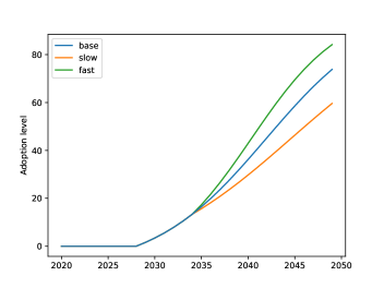
Figure 1: Illustration of a Bass diffusion process $A_{mfs}(\tau)$ from (13) starting in year $\bar{\tau}_{mf}=2028$. Plotted are a base scenario with constant $\alpha$ and $\beta$ parameters, as well as a slow and fast scenario, with a decrease and increase, respectively, in these parameter values by 25% in the year 2034.

We use this diffusion model to derive two constraints in our model that constitute upper bounds on both the adoption level of technology $(m,f)$ and its rate of change. First, we use the theoretical value $A_{mfs}(\tau)$ from the Bass diffusion above as an upper bound on the actual adoption share $\frac{\tilde{q}_{mf\tau s}}{\tilde{q}^{\text{tot}}_{m\tau s}}$ of technology $(m,f)$ in our model. That is, we add the constraint:

$$\tilde{q}_{mf\tau s}\leq A_{mfs}(\tau)\tilde{q}^{\text{tot}}_{m\tau s}.$$ (14)

Thus, the diffusion model represents the fastest possible adoption path for the technology. The reason we only use this as an upper bound is that we do not wish to force the adoption of any technology; the model should be free to choose what technologies to use.

A caveat of this constraint is that it does not directly limit the rate of adoption. For instance, if the actual adoption starts later than at time $\bar{\tau}_{mf}$, then the adoption rate may “jump” from zero to a high value if we do not add any additional constraints. To mitigate this issue, we add another constraint that restrict the rate of adoption, especially in early stages of the adoption process. Again, we base this on the Bass diffusion model. As a starting point, we take the Bass equation:

$$\frac{\frac{d}{d\tau}F_{mfs}(\tau)}{1-F_{mfs}(\tau)}=\alpha_{mfs}(\tau)+\beta_{mfs}(\tau)F_{mfs}(\tau).$$ (15)

Our aim is to translate this non-linear differential equation into a linear constraint that we can add to our model. First, we change the equality by an inequality (to yield an upper bound on the rate of adoption) and approximate the differential equation by a difference equation, yielding:

$$\frac{F_{mfs}(\tau)-F_{mfs}(\tau-1)}{1-F_{mfs}(\tau-1)}\leq\alpha_{mf,\tau-1,s}+\beta_{mf,\tau-1,s}F_{mfs}(\tau-1),$$ (16)

where $\alpha_{mf\tau s}:=\alpha_{mfs}(\tau)$ and $\beta_{mf\tau s}:=\beta_{mfs}(\tau)$, $\tau\in\mathcal{T}$. This constraint is nonlinear in $F_{mfs}(\tau-1)$ due to the fraction on the left-hand side. Note that we are mainly interested in limiting the rate of adoption in early stages of the adoption path, i.e., when $F_{mfs}(\tau-1)$ is close to zero, i.e., when $1-F_{mfs}(\tau-1)$ is close to one. Thus, we can approximate the inequality above by ignoring the factor $1-F_{mfs}(\tau-1)$ in the denominator:

$$F_{mfs}(\tau)-F_{mfs}(\tau-1)\leq\alpha_{mf,\tau-1,s}+\beta_{mf,\tau-1,s}F_{mfs}(\tau-1).$$ (17)

Writing this in terms of the adoption level $A_{mfs}(\tau)=U_{mf}F_{mfs}(\tau)$, using the equality $A_{mfs}(\tau)=\frac{\tilde{q}_{mf\tau s}}{\tilde{q}^{\text{tot}}_{m\tau s}}$, we obtain:

$$\frac{1}{U_{mf}}\left(\frac{\tilde{q}_{mf\tau s}}{\tilde{q}^{\text{tot}}_{m\tau s}}-\frac{\tilde{q}_{mf,\tau-1,s}}{\tilde{q}^{\text{tot}}_{m,\tau-1,s}}\right)\leq\alpha_{mf,\tau-1,s}+\frac{\beta_{mf,\tau-1,s}}{U_{mf}}\frac{\tilde{q}_{mf,\tau-1,s}}{\tilde{q}^{\text{tot}}_{m,\tau-1,s}}.$$ (18)

Approximating $\tilde{q}^{\text{tot}}_{m\tau s}$ by $\tilde{q}^{\text{tot}}_{m,\tau-1,s}$ (which we expect to be quite close), and multiplying both sides by $U_{mf}\>\tilde{q}^{\text{tot}}_{m,\tau-1,s}$, we obtain:

$$\tilde{q}_{mf\tau s}-\tilde{q}_{mf,\tau-1,s}\leq\alpha_{mf,\tau-1,s}\>U_{mf}\>\tilde{q}^{\text{tot}}_{m,\tau-1,s}+\beta_{mf,\tau-1,s}\>\tilde{q}_{mf,\tau-1,s}.$$ (19)

This is the inequality that is included in STraM. Note that, similar to the Bass model, it limits the rate of adoption $\tilde{q}_{mf\tau s}-\tilde{q}_{mf,\tau-1,s}$ of fuel technology $f$ on mode $m$ by the sum of two terms: one depending on the current adoption level $\tilde{q}_{mf,\tau-1,s}$ of fuel technology $f$, and one independent of the current adoption level.

4.2 Path generation

Our path-flow model formulation requires the a priori generation of a set of admissible paths. That is, for every origin-destination pair $(o,d)\in\mathcal{N}\times\mathcal{N}$, we need to generate a collection of paths that can be used to transport goods from $o$ to $d$. To keep the model size manageable, we only generate a limited number of “reasonable” paths, which is common practice in multimodal transport network design models (de Jong et al., 2013a; Van Riessen et al., 2015; Zhang et al., 2008). Here, we describe the process we use to generate these paths.

The main criterion we use for generating paths is the cost of transporting one tonne of goods over that path. Only the cheapest possible paths are included in the set of admissible paths. However, we want our path generation procedure to be agnostic about the choice of modes in the path. Hence, for every origin-destination pair, we generate a cheapest path for every sequence of modes (e.g., road–sea) from a predefined set of admissible sequences. In particular, we allow all sequences of modes that consist of at most two modes.

To compute the cheapest paths, we follow a procedure from the “BuildChain” module in the the Norwegian National Freight Model System (de Jong et al., 2013a). First, we compute all unimodal cheapest paths (i.e., paths using only one transport mode $m\in\mathcal{M}$) by means of Dijkstra’s shortest path algorithm (Dijkstra, 1959). Then, to compute the cheapest two-mode path from $o\in\mathcal{N}$ to $d\in\mathcal{N}$ using the mode sequence $(m_{1},m_{2})$, we only need to find the optimal transfer node $n\in\mathcal{N}$. Using the already computed cheapest unimodal paths, the cost of the path from $o$ via $n$ to $d$ simply consists of the cost of the cheapest unimodal $m_{1}$-path from $o$ to $n$ plus the cost of the cheapest unimodal $m_{2}$-path from $n$ to $d$. Looping over all possible transfer nodes $n\in\mathcal{N}$ and picking the transfer node with the lowest total cost yields the cheapest $(m_{1},m_{2})$-path. An analogous procedure can be used to find the cheapest three-mode paths: here we need to find the optimal transfer node $n$ where we split the three-mode path into a unimodal $m_{1}$-path from $o$ to $n$ and a two-mode $(m_{2},m_{3})$-path from $n$ to $d$. Again, the costs of these subpaths have already been calculated before.

One difficulty in generating the cheapest paths in this way is the fact that in our model, the cost of transporting goods over a given path depends on various factors. First, the cost of transporting a tonne of goods over a given arc $a\in\mathcal{A}$ in the path with corresponding mode $m\in\mathcal{M}$ depends on (1) the vehicle used that mode (which we assume to directly depend on the product type $p\in\mathcal{P}$), (2) the fuel $f\in\mathcal{F}_{m}$ used in the vehicle, and (3) the cost scenario $s\in\mathcal{S}$. Second, the cost of transferring goods from one mode to another along the path also depends on the product group $p\in\mathcal{P}$. These dependencies make the path costs ambiguous and hence, make it unclear what path should be deemed cheapest and added to the set of admissible paths.

A limited version of this issue has been recognized by Zhang et al. (2008), who consider a model where path costs also depend on the product type (but not on fuels or scenarios). Their solution to the issue is simple: find the cheapest path for every given product type $p\in\mathcal{P}$ and add all the generated paths to the set of admissible paths. We follow this idea and generate paths for every possible combination of product type $p\in\mathcal{P}$, fuel $f\in\mathcal{F}_{m}$ for each mode $m\in\mathcal{M}$, and scenario $s\in\mathcal{S}$. Hence, in total our path generation algorithm is run $|\mathcal{P}|\times\sum_{m\in\mathcal{M}}|\mathcal{F}_{m}|\times|\mathcal{S}|$ times. Note, however, that in many runs the same paths are found, so the resulting total number of paths remains limited.

4.3 Scenario generation

To explicitly account for the uncertainty in the development of new fuel technologies in our model, we define a set of scenarios with associated probabilities. Every scenario represents one possible realization of the development of all fuel technologies in terms of their adoption level (according to the associated Bass diffusion process) and their associated levelized cost of transport. Here we describe how we generate these scenarios.

First, we define a base development path for every technology (i.e., for every mode-fuel combination $(m,f)$), representing a prediction of its development, based on the most reliable data, forecasting models, and expert opinions that are available. Next, we generate alternative development paths by varying a number of relevant parameters by a predetermined amount, to create optimistic and pessimistic development paths. In particular, we vary the generalized transport costs $C_{afpts}$ and the technology adoption parameters $\alpha_{mfts}$ and $\beta_{mfts}$ associated with a technology $(m,f)$. The deviations we use are presented in Table 4. These parameter changes take place starting in 2034, i.e., at the start of the second stage in our stochastic program. Before 2034, the values are the same for all scenarios.

	$C_{afpts}$	$\alpha_{mfts}$	$\beta_{mfts}$
Optimistic	$+25\%$	$+25\%$	$+25\%$
Pessimistic	$-25\%$	$-25\%$	$-25\%$

Table 4: Parameter deviations in optimistic and pessimistic development paths, relative to the base path.

Every technology $(m,f)$ has its own cost and technology adoption parameters that can be varied. However, to keep the number of scenarios limited, we vary these parameters by fuel group. These are groups of mode-fuels that make use of similar technologies, whose technological development can be expected to be correlated. In our case study we define four technology groups: established technologies, battery-based technologies, hydrogen technologies, and biofuel technologies; see Table 6 in Section 5 for more details. Of these, we keep the technologies in the established group fixed at their base path, while varying the other technology groups. Generating all combinations of optimistic, and pessimistic development paths, besides a base scenario we obtain a limited number of $2^{3}+1=9$ scenarios. The scenario tree is illustrated in Figure 2.

Figure 2: Schematic illustration of the scenario tree used in STraM. The scenario names consist of three letters, corresponding to the fuel groups battery-based, hydrogen-based and biofuels, respectively, indicating whether for that fuel group the optimistic (O), base (B), or pessimistic (P) case is active in the scenario.

5 Numerical illustration: Norway

To illustrate the capabilities of STraM, we provide a numerical illustration using a case study of the Norwegian freight transport system. We describe the case study in Section 5.1, and we discuss our analysis and results in Section 5.2.

5.1 Case description

We consider the development of the Norwegian transport system for discrete time periods $\left\{2023,2028,2034,2040,2050\right\}$, where the underlying transport network is summarized in Figure 3. The nodes represent the main cities/capitals for the counties in Norway, along with Northern-Sweden (represented by Umeå) and Southern-Sweden (represented by Stockholm), the Norwegian Continental Shelf (for oil and gas production), mainland Europe and the rest of the World.

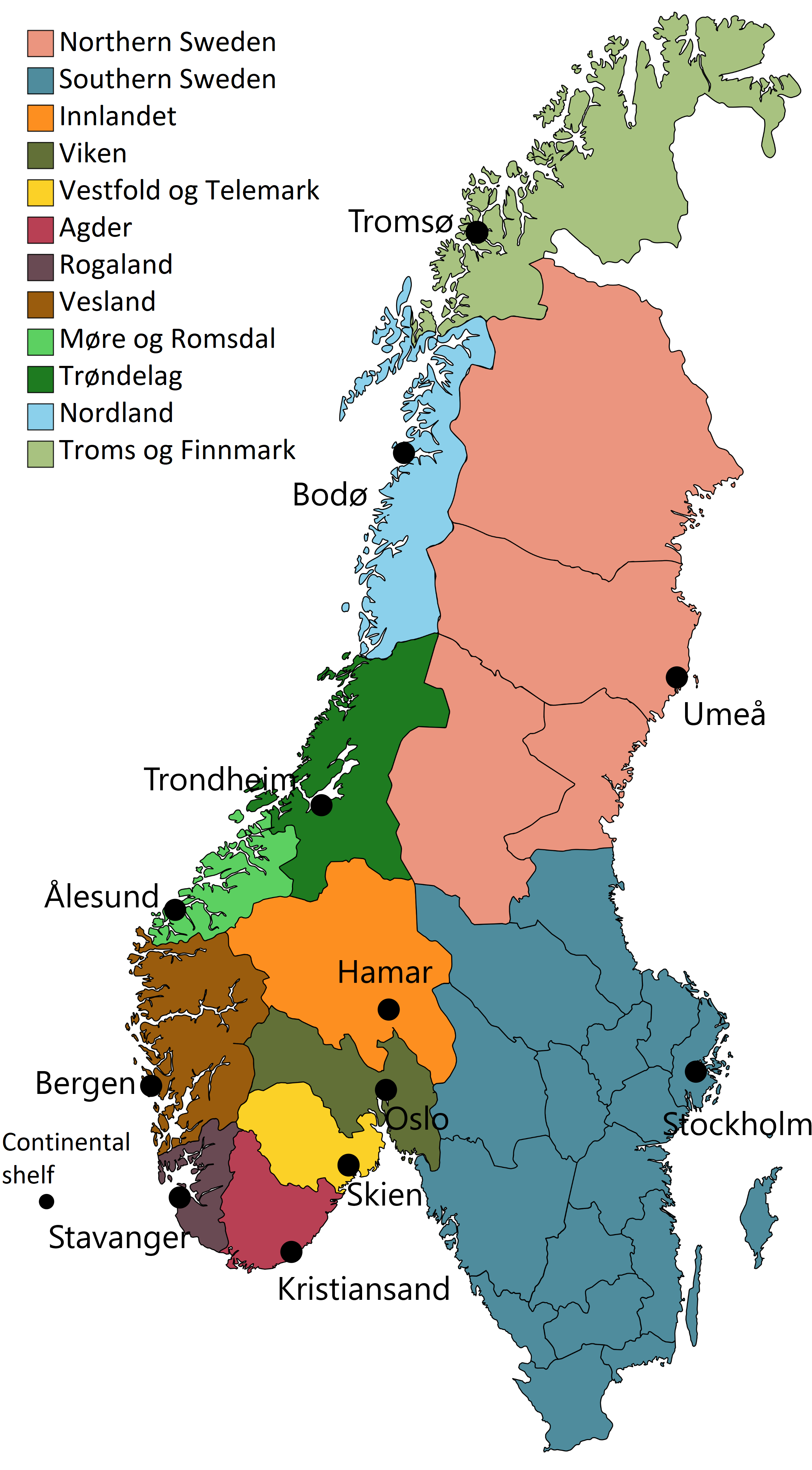
(a) Regions

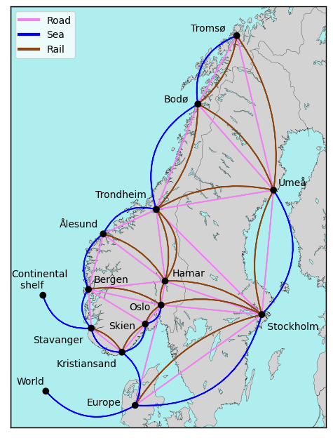
(b) Network

Figure 3: The considered network. Figure 3(a) shows the mapping from regions/counties to nodes, while Figure 3(a) visualizes the transport network that we consider.

Undirected edges are defined between all feasible combinations of nodes (cities/areas), modes (rail, road, sea) and routes. The edges therefore represent the main transport corridors. As an example, transport between Trondheim and Bodø can be performed on road, rail and sea. Hence, we include three distinct edges between these nodes. Contrarily, sea transport is not possible between Hamar and Trondheim, but there are two different rail lines (or routes) that can be used, namely, Dovrebanen and Rørosbanen. We note that some links are not yet established (e.g. rail between Bodø and Tromsø). But, investments in these links can increase capacity and lead to positive flows. Based on the developed network, the path generation algorithm outlined in Section 4.2 generates $3030$ unique paths between the nodes in the system, when allowing for a single mode shift.

The network is used to satisfy the demand for the transport from an origin node to a destination node for the following six product groups (commodities): dry bulk, fish, general cargo, industrial goods, thermo and timber. We note that we excluded wet bulk as it mainly consists of transport of hydrocarbons from the Norwegian Continental Shelf that have a dedicated value chain. We consider demand for long-distance transport between counties, but not short-distance transport within counties (which we assume to a large extend will be electrified). The (remaining) transport amount (in Tonnes) is visualized in Table 5 and Figure 4.

Table 5: Annual transport demand (in megatonnes) in each time period.

Year	2022	2026	2030	2040	2050
Demand (in MTonnes)	129.6	152.0	167.2	175.3	196.4

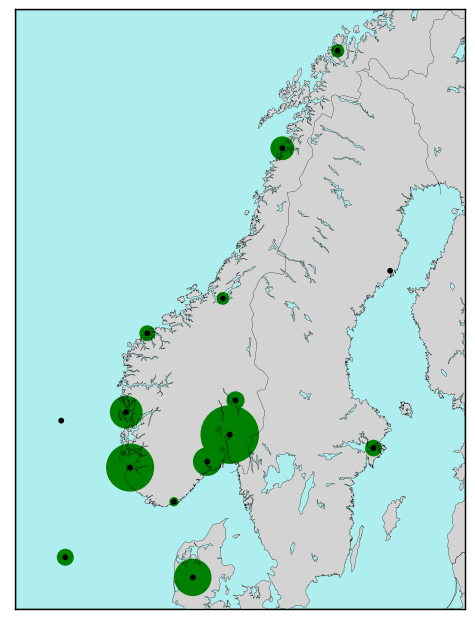
(a) Origin

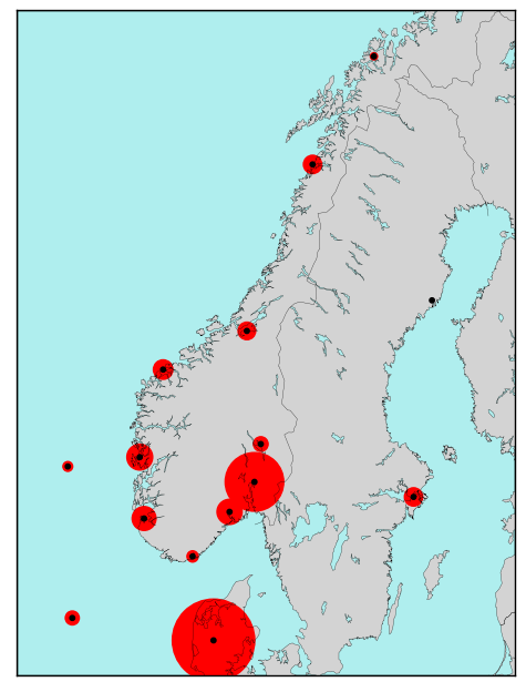
(b) Destination

Figure 4: Visualization of the transport demand matrix for 2022.

Moreover, the modes of transport can use different fuel technologies, including Heavy Fuel Oil (HFO), Marine Gas Oil (MGO), Liqued Natural Gas (LNG), Contact Line Electric Train (CL), Hydrogen (H2) and Ammonia (NH3). Table 6 presents an overview over the different configurations that we consider.

Table 6: Mode-fuel combinations and fuel groups.

	Established					Battery-based		H2-Based		Biofuels
	HFO	MGO	LNG	CL	Diesel	Battery	Hybrid	H2	NH3	Bio- diesel	Bio- gas
Rail				x	x	x	x	x		x
Road					x	x		x		x	x
Sea	x	x	x					x	x	x	x

The table allocates the fuel technologies to one of the four technology groups defined in Section 4.3: established technologies, battery-based technologies, hydrogen technologies, and biofuel technologies.

The underlying parameter values that we use (e.g., transport costs, capacities and investments) are openly available on GitHub (Bakker & van Beesten, 2023). Moreover, we have listed all references that were used to construct this dataset in A. For a more extensive description of the data used, we refer to Brynildsen et al. (2022), which contains an earlier version of the case study.

5.2 Results

In this section, we present computational results for the model developed in Section 3 and Section 4, using the case study as described in Section 5.1. The model is implemented in Python 3.10.4, formulated using Pyomo and solved using Gurobi 10.0. The model is openly available on GitHub (Bakker & van Beesten, 2023). The analysis are carried out on a Lenovo NextScale nx360 M5 server with an Intel E5-2643v3, 2x3.4 GHz processor, 512Gb RAM, running CentOS 7.9.2009 and using up to twelve threads. The extensive form of the model with $9$ scenarios consists of $94,874$ constraints, $552,098$ continuous variables and $762$ binary variables after pre-solve. It solves in approximately $1$ hour with an optimality gap of $0.5\%$ .

5.2.1 Base case

We first discuss general findings observed in the base case, which corresponds to the model (1)-(12m) with the data described in Section 5.1 and risk parameters $\lambda=0.2$ and $\gamma=0.8$. We visualize the results in various ways. First, we break down the objective function in its cost components. Figure 5(a) shows the one-time investment costs in each time period.

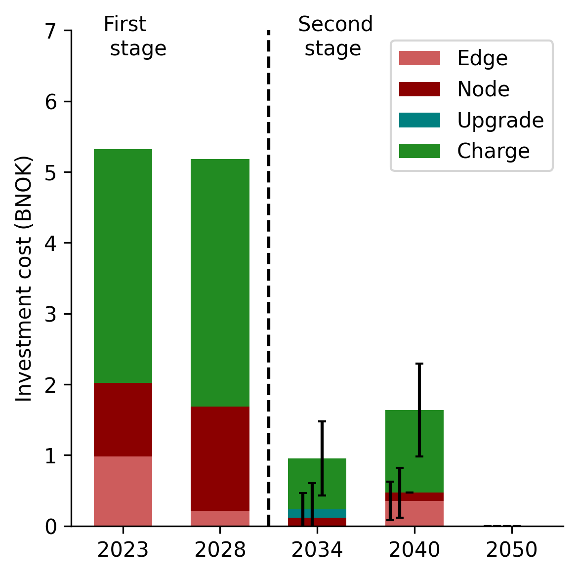
(a) Investments

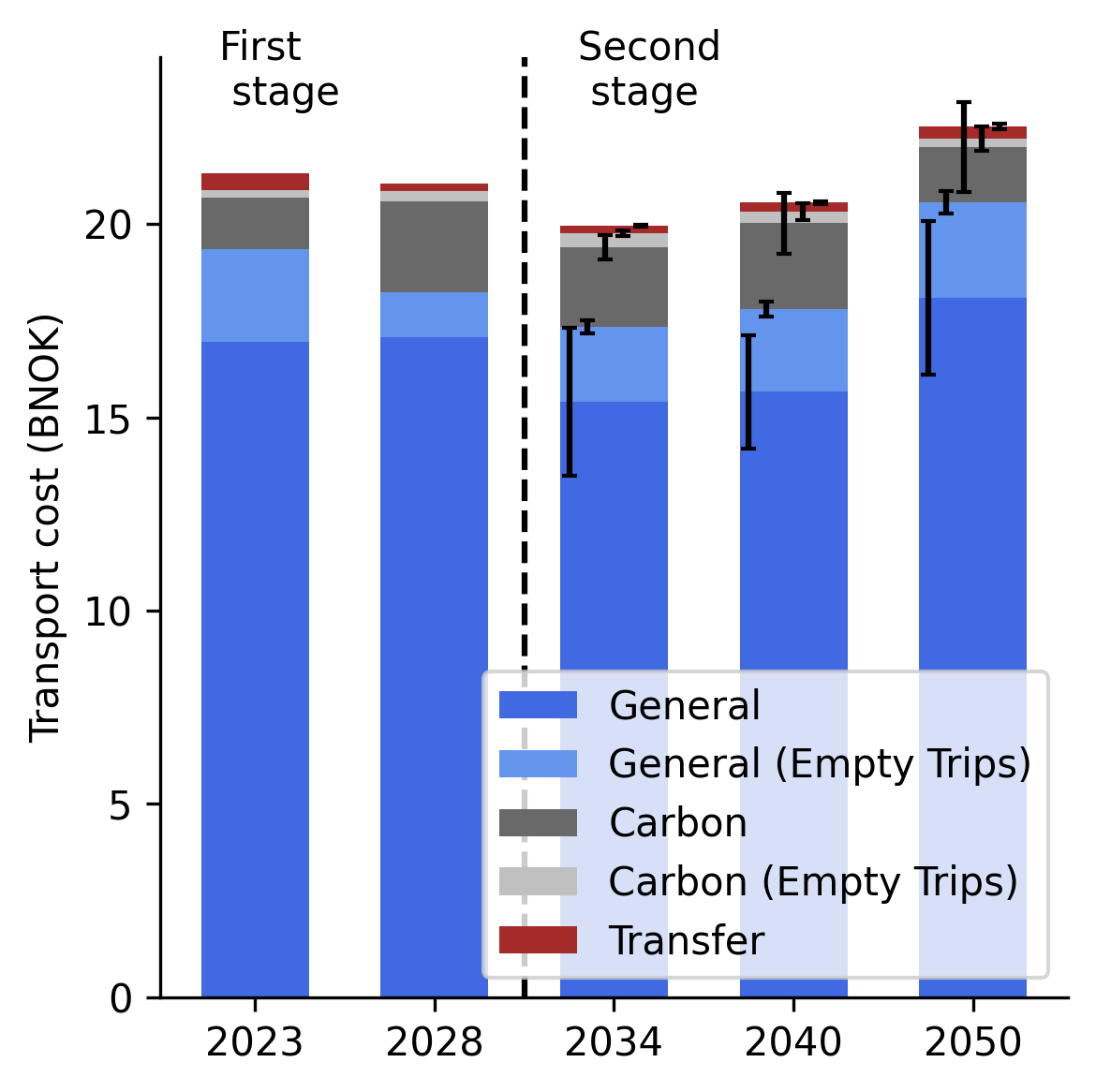
(b) Transport costs

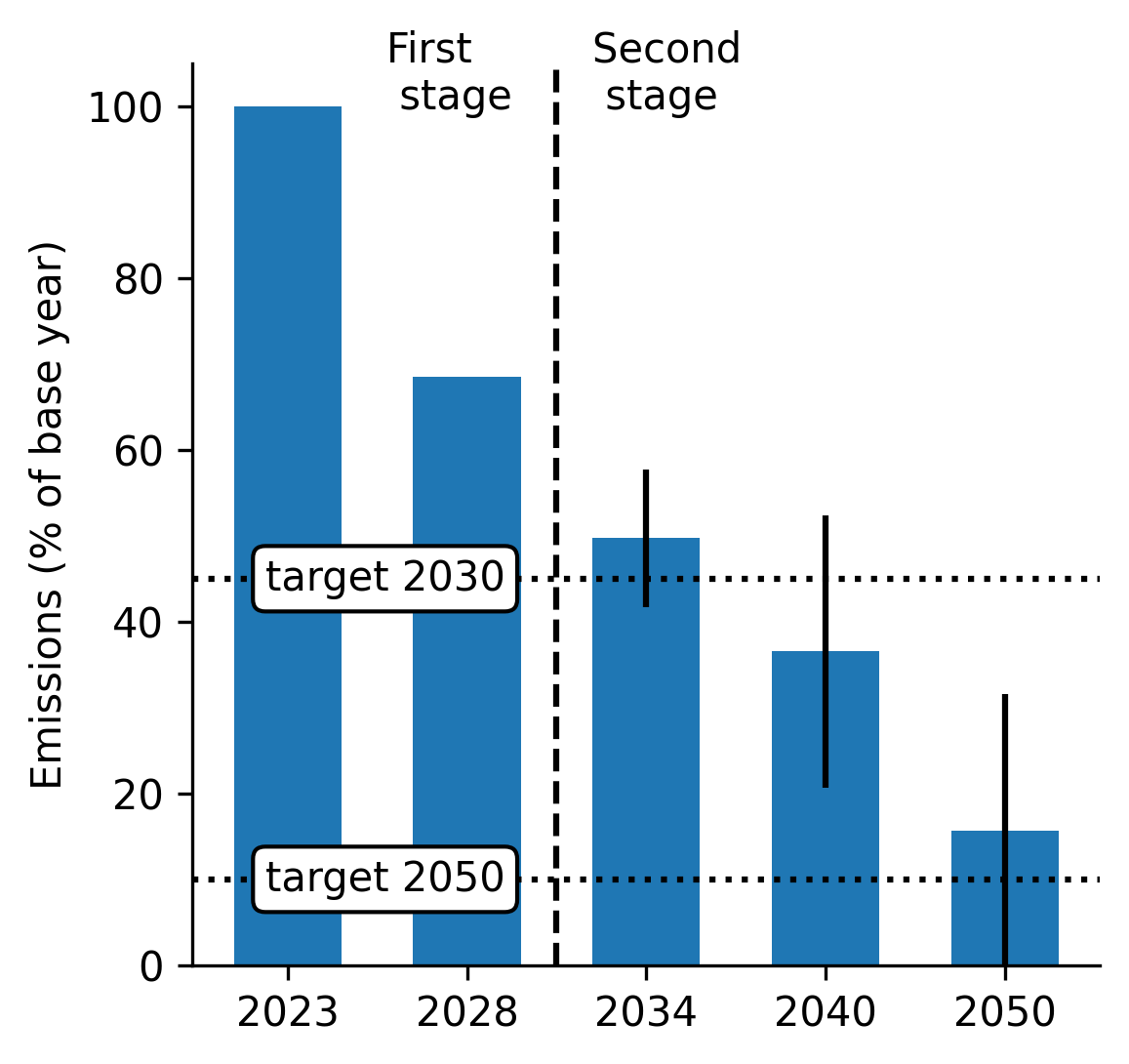
(c) Emissions

Figure 5: Cost structures for (5(a)) investments and (5(b)) transport, where the carbon costs are extracted from the generalized transport costs. Implied emissions (relative to the base emissions in 2023) are presented in (5(c)). The black error bars denote standard deviations.

In the first stage, investments are made in charging and filling infrastructure on road, upgrading railway lines from diesel to contact-line electric and expanding terminal capacity in some of the nodes. Moving to the second stage, we observe that the level of investments depends on the scenario (realization of uncertainty), in particular for investments in charging infrastructure on road. From Figure 5(b) we see that there is an initial decrease in the (generalized) transport costs. This can be explained by sustainable fuels, in particular battery technologies, becoming increasingly competitive over time. Eventually, the transport costs increase, as rising carbon prices force more expensive low-carbon mode-fuel combinations into the transport mix, at the cost of fossil fuels. Nevertheless, we see that the share of carbon costs to operational costs stays fairly constant. Finally, we note that the empty, balancing, trips account for a significant amount of the costs, and should not be neglected.

The increasing carbon price, is responsible for a growing share of sustainable fuels in the optimal mode-fuel split . Figure 5(c) shows the implied emissions for the base case and compares it with targets set by the Norwegian government. Despite a significant decrease in emissions over time, we observe that for the majority of scenarios the targets are not achieved.

Figure 6 shows significant changes in the mode-fuel split over time.

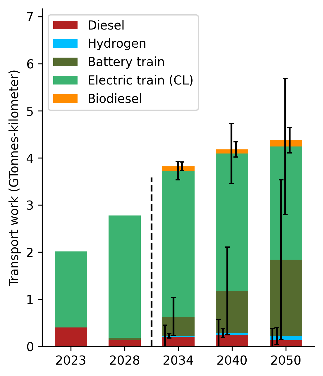
(a) Rail

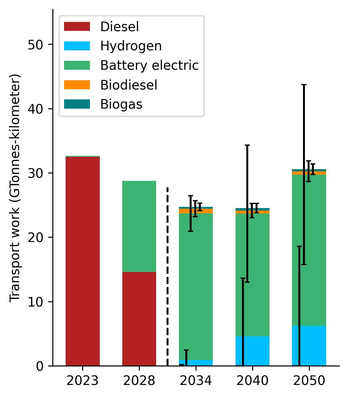
(b) Road

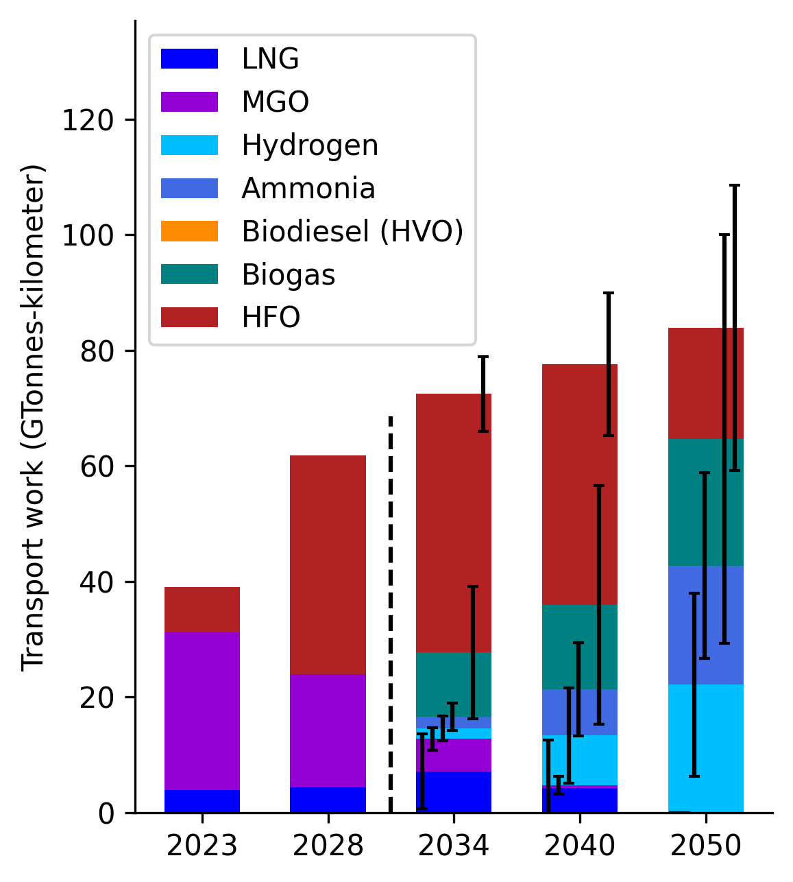
(c) Sea

Figure 6: Mode-fuel splits for the different transport modes. Standard deviations of second stage results are visualized using black error bars.

From Figure 6(b) we see that the transport share on road decreases during the first time periods. The main explanation here is that, rail and sea transport are a more cost-efficient solution mode of transport for certain product groups in the short term, as is confirmed visually in Figures 6(a) and 6(c) through the increasing mode shares. Another factor is that the technology adoption constraints (10) limit the adoption of new technologies. Furthermore, we observe that transport on rail is initially at maximum capacity. But due to the edge investments and upgrades visualized in Figure 5(a), the total amount of transport work increases monotonically over time. For sea transport we observe that the transition to low-carbon fuels is slow. This is a consequence of the fact that these fuels become competitive relatively late, in combination the fleet renewal constraints, which have a strong effect due to the fact that ships have long lifetimes. Common across all modes of transport is the fairly high level of uncertainty in the future mode-fuel splits. Most fuels are being used in some future scenario realization, but the level of adaption strongly depends on the realization of uncertainty. This in turn can have significant impact on the infrastructure investments in the first stage. For example, investments are made in charging and filling infrastructure for battery electric as well as fuel-cell electric trucks.

Next, we analyze geographical properties of our solutions.

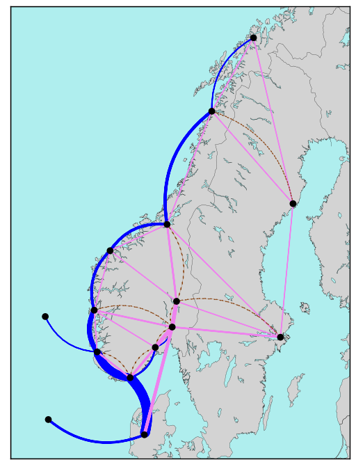
(a) Flow in 2023 by mode.

(b) Change in flow from 2023 to 2050 (green represents an increase, red represents a decrease in aggregate flow).

(c) Flow of fish in 2050 by mode in the base scenario

(d) Flow of Timber in 2050 by mode in the base scenario.

Figure 7: Geographical plots of flow of goods. The thickness of each edge is proportional to the aggregated flow of goods in tonnes in both directions; these thicknesses are normalized for each plot separately. Curved blue edges represent sea, straight pink edges represent road, curved, dashed, brown edges represent rail.

In Figure 7 we plot the flow of goods on a map. Figure 7(a) shows the mode split of the aggregate flow over all product groups in 2023. Coastal transport tends to make use of sea, while inland transport tends to use road as the preferred mode of transport. The overall picture for 2050 looks similar. However, some interesting changes can be observed in Figure 7(b). In the base scenario, the pattern described above is even more pronounced in 2050: more sea is used for coastal transport, at the cost of road, while more road is used for inland transport. Besides, there are some increases in rail transport. Figure 7(c)–7(d) illustrates that the choice of transport mode varies significantly by product group: for example, fish is transported mostly by sea, while timber is transported mostly by road.

In Figure 8 we plot the investments in charging infrastructure for battery-electric trucks in the first-stage years 2023 and 2028.

(a) 2023

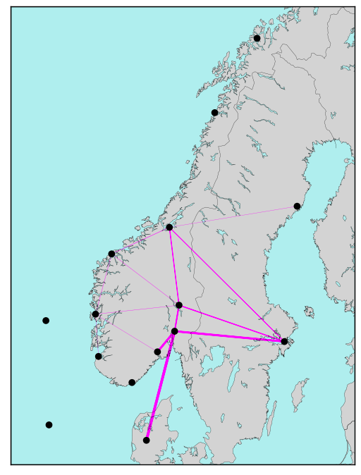
(b) 2028

Figure 8: Geographical plot of optimal charging infrastructure investments for battery-electric trucks in 2023 and 2028. The thickness of each edge represents the investment level in tonnes of capacity.

In 2023, investments mainly take place on the inland route Bergen – Oslo – Hamar – Trondheim and on the connections from South-Sweden to the neighboring Norwegian nodes. The explanation for these investments is that for geographical reasons, the relevant road connections are much shorter than connections by sea, which is the main competitor mode. Elsewhere in the network, the availability of short sea connections makes investments in road infrastructure less attractive. In 2028 we see a similar pattern, but with additional investments on the edge from Oslo to Europe and along coastal edges.

5.2.2 The value of uncertainty

In this section we evaluate the effect of including uncertainty in our model and quantify the extend to which this improves the solution. First, we compare the results from our stochastic programming solution (SP) in the base case, with the so-called expectation of the expected value solution (EEV) (Birge, 1982). The expected value solution (EV) solves a deterministic model with all uncertain parameters equal to their expected (base) values. The EEV then solves the stochastic model, but fixes the first stage decisions from the EV. Figure 9(a) and Figure 9(b) present the resulting investment costs for the SP and EEV, respectively.

(a) SP

(b) EEV

(c) Risk-neutral

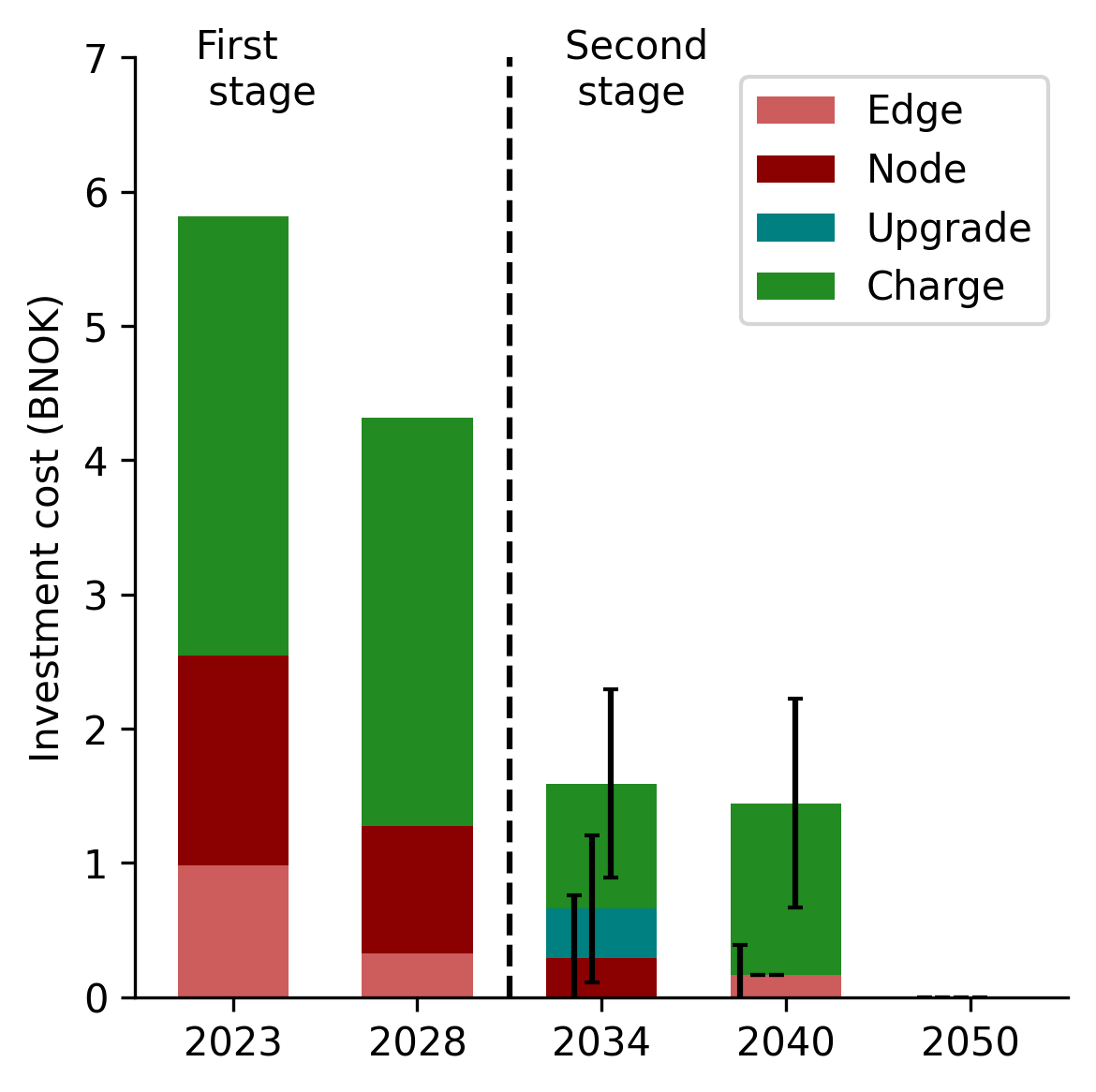
(d) Maximally risk-averse

Figure 9: Investment cost structures for (9(a)) the SP solution; (9(b)) the EEV solution; (9(c))a risk-neutral case, and (9(d)) a maximally risk-averse case. Capacity increasing investments can be made in edges for rail (Edge) or road (Charge) or in terminals (Node). Upgrade enables the use of new technologies on rail. The black error bars denote standard deviations.

We observe that the EEV invests more and earlier. The SP rather waits a bit more and postpones some investments to the second stage, when uncertainty is realized. This flexibility gives a monetary gain that can be quantified using the value of stochastic solution (VSS), defined as the difference between the SP and EEV. With a discounted system cost of $615.65$ Billion Norwegian kroners (BNOK) for the SP, and $655.15$BNOK for the EEV, this implies a VSS of $6.03\%$. In addition, the average total emissions (across all scenarios) are $32$ thousand Tonnes CO₂ lower for VSS than EEV ($4.86\%$).

Figures 9(c) and 9(d) show the investment costs when solving the model using a risk neutral objective function (only using the expected value) and a maximally risk-averse objective function (only counting the worst scenario). Compared to the base case with modest risk aversion, the risk neutral case in general invests less. For the maximally risk-averse case, investments are, in general, made earlier and the magnitude of investments is higher. Thus, risk is mitigated by investing early.

5.2.3 Carbon price sensitivity

Figure 5(c) showed that with the given carbon price, in most scenarios the emission targets are not reached. We perform a sensitivity on these carbon prices to show its effectiveness as a political instrument. Figure 10(a) and 10(b) present the emissions when the carbon price is set to zero, or when the carbon price is doubled, respectively.

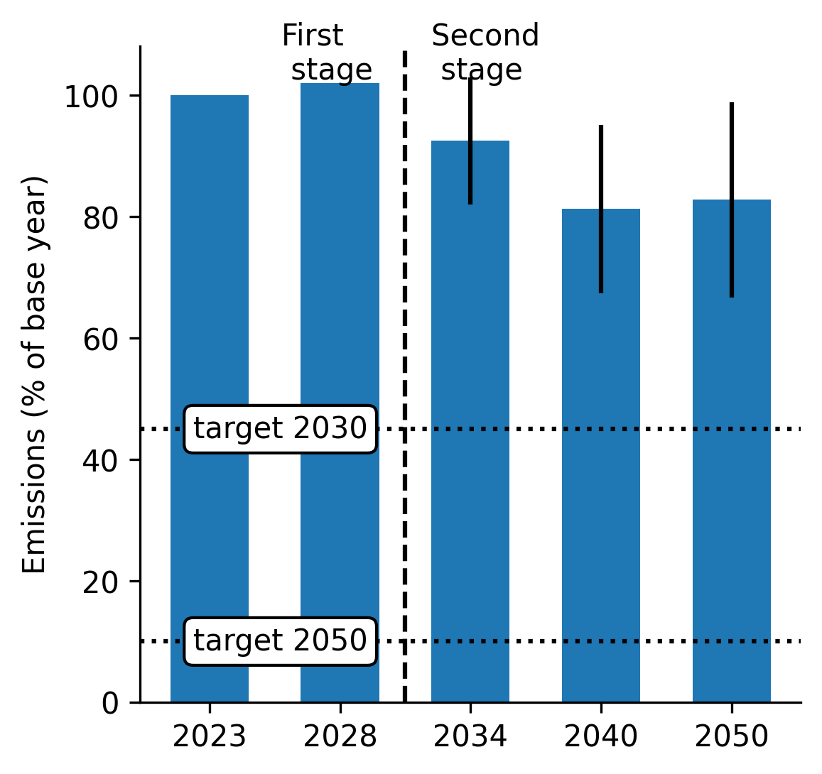
(a) No carbon price

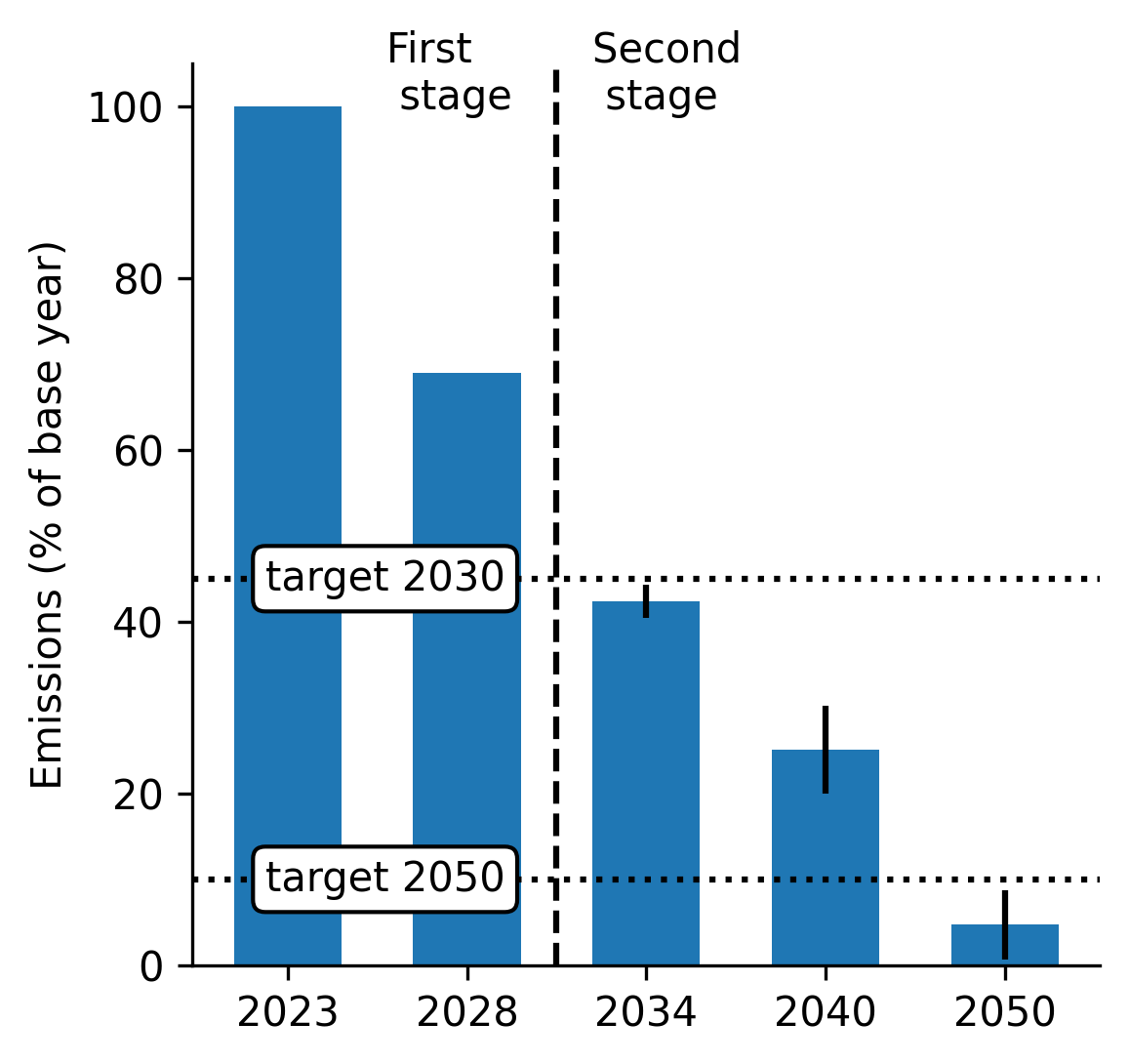
(b) Double carbon price

Figure 10: Emissions for a case with no carbon price (10(a)) and a doubling in the carbon price (10(b)). The black error bars denote standard deviations.

Figure 10(a) clearly shows that, despite showing a modest decrease in emissions, a significant carbon price is needed to come anywhere near the emission targets. Doubling the carbon price relative to the base values, ensures that emission targets are reached from $2034$ and on-wards. Nevertheless, due to technology adoption and fleet renewal constraints, the $2030$ target of $55\%$ emission reductions might be difficult to achieve much earlier than $2034$, despite high carbon prices. When inspecting the mode-fuel splits, the most striking behaviour is on sea, where HFO turns out to take the whole share of maritime transport in $2050$. In contrast, when doubling the carbon price, HFO almost completely diminishes from the mix.

5.2.4 Static model comparison

A common approach to performing strategic analyses with the existing static transport models is to solve the static model for a given time period in the future using fixed parameter forecasts (see e.g., Crainic et al. (1990b); Pinchasik et al. (2020)). Such an approach neglects temporal dependencies, such as fleet renewal and technology adoption, but rather focuses on finding the optimal fleet mix in a given year. To illustrate some of the differences with such an approach, we mimic the static modeling behaviour by neglecting all operational constraints except for the year of interest. We note that we do allow for investments in all time periods. Figure 11 compares the mode-fuel split resulting from the static run with the base case for $2034$ as well as $2050$.

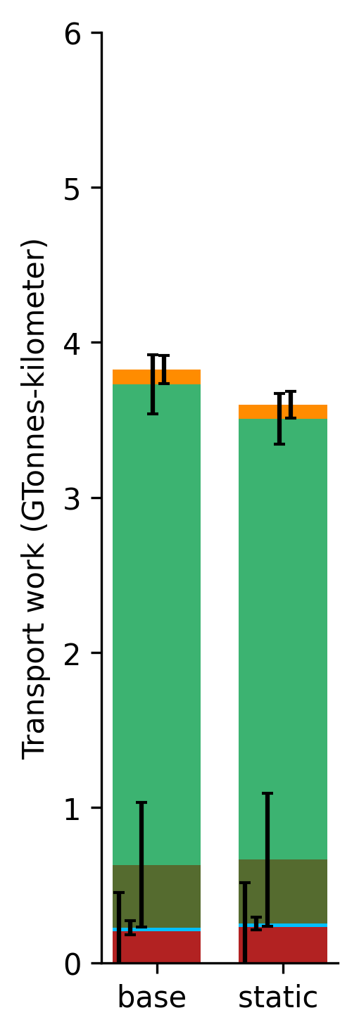
(a) Rail, 2034

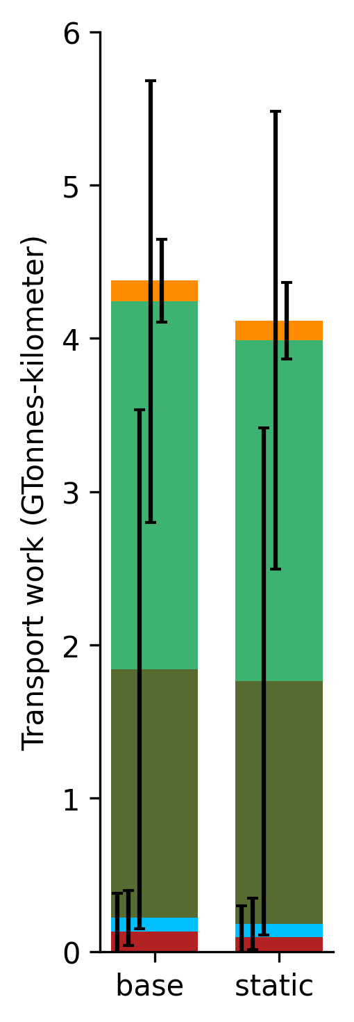
(b) Rail, 2050

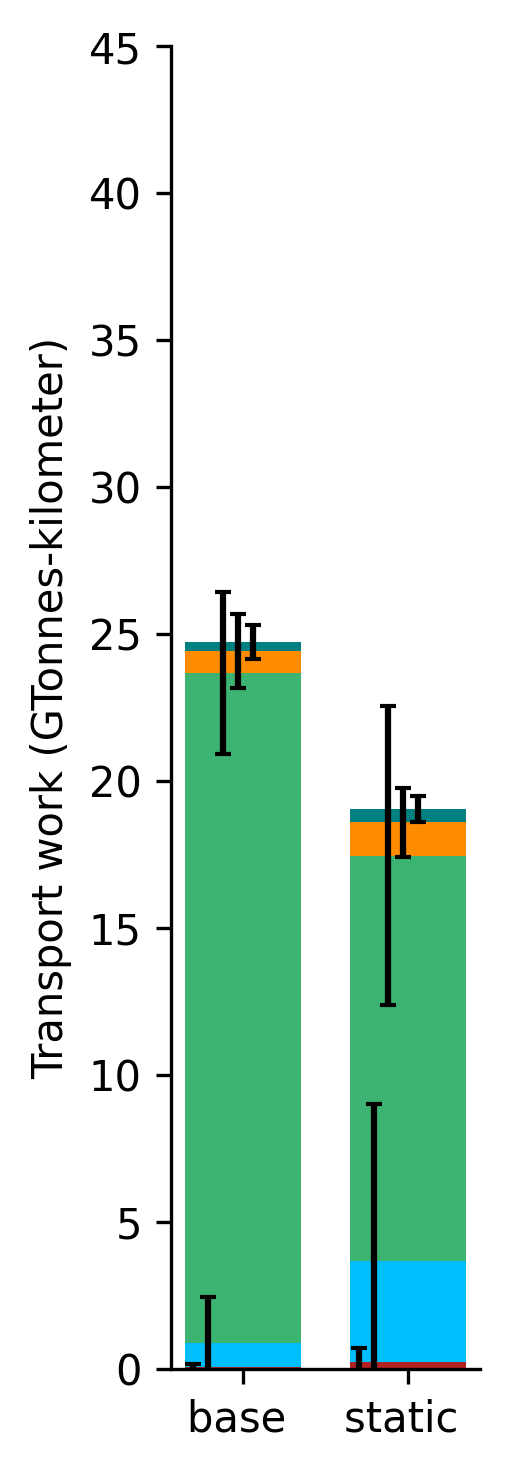
(c) Road, 2034

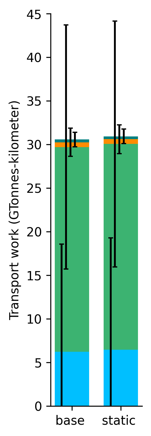
(d) Road, 2050

(e) Sea, 2034

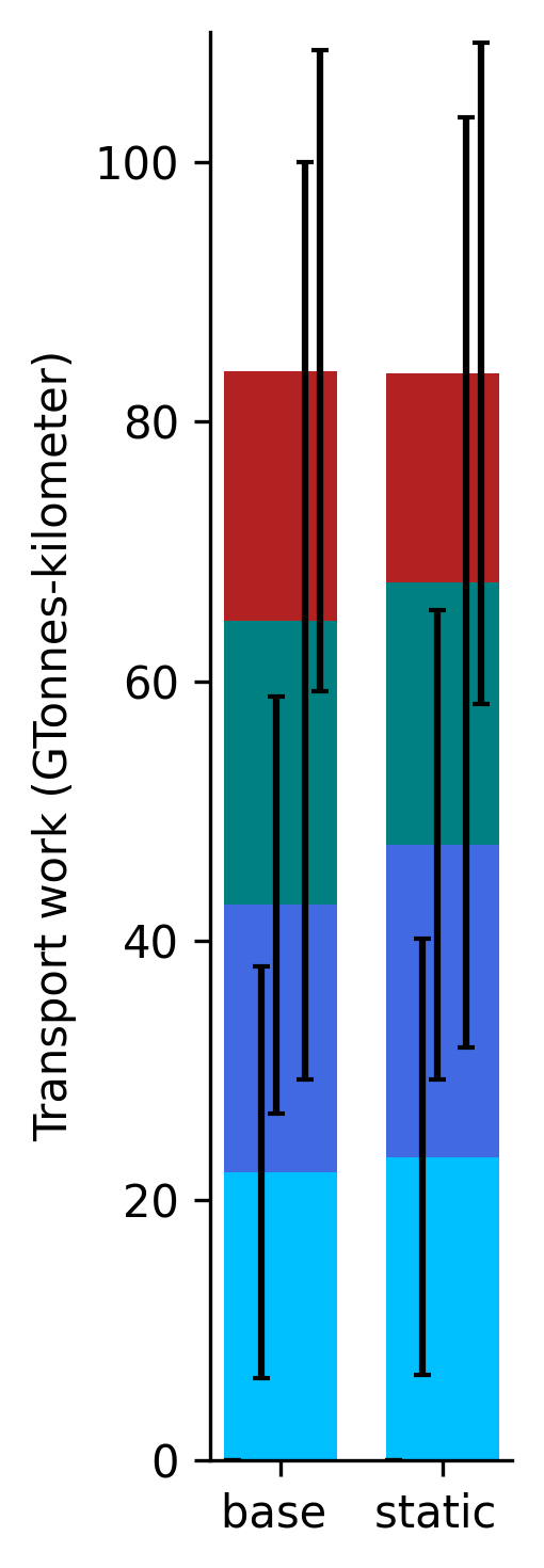
(f) Sea, 2050

Figure 11: Mode-fuel splits in 2034 and 2050 for base and static case.

We observe that while the fleet mixes are nearly identical in $2050$, the fleet mixes differ significantly in $2034$. Thus, both approaches mostly agree on what the system should look like by 2050, but the static model fails to anticipate for this future system when optimizing for the year 2034. Moreover, static approaches only manage to highlight the existence of infrastructure in a given year. In contrast, STraM provides information on the exact timing of long-term investments. Overall, this shows the relevance of a dynamic, multi-period approach, that takes into account fleet renewal and technology adoption constraints.

6 Conclusion

In this article, we have presented STraM, a framework for strategic national freight transport modeling. By explicitly accounting for the dynamic nature of long-term planning, as well as the development and adoption of new fuel technologies with corresponding uncertainties, STraM is tailored to identify decarbonization pathways and evaluate the impact of government or industry policies. To be able to include these strategic elements, we sacrifice some of the more detailed logistics elements (such as consolidation) that are implemented in the current state-of-the-art national freight transport models. We believe that this is an acceptable limitation as our focus lies on evaluating long-term investments. Moreover, by explicitly modeling the flow of goods in the system in each time period, we still obtain a good approximation of the performance of the operations.

To evaluate the developed framework, we constructed a case study for the freight transport sector in Norway. Our results show that the commonly used what-if approach does not manage to consider technology adaption and fleet renewal, leading to a forecasted transport system that is considerably different from the optimal system that results from STraM. This clearly illustrates the need for a dynamic, multi-period, transport model. Moreover, we find that the explicit consideration of uncertainty in transport costs and technology development leads to a significant improvement in results. In particular, we identify a value of the stochastic solution of approximately $6\%$. An interesting result from a policy-maker point of view is that a carbon price proves to be an efficient measure to reach emission targets, although relatively high prices are needed. Furthermore, we find that investment patterns differ both spatially and temporally. Overall, we conclude that all of the methodological contributions, i.e., the consideration of multiple time periods with endogenous infrastructure investments; description of (new) fuel technology adoption; and long-term technology- and cost-uncertainty, contribute to better strategic freight transport modeling.

In future work we will use STraM for policy-oriented analyses. We are currently in the process of validating and aligning data input with various industry actors and research institutions. Moreover, we want to investigate the relationship with energy infrastructure that currently falls outside of the scope of the model.

CRediT authorship contribution statement

Steffen J. Bakker, E. Ruben van Beesten: Conceptualization, Methodology, Software, Formal Analysis, Visualization, Writing - original draft Ingvild Synnøve Brynildsen, Anette Sandvig, Marit Siqveland: Conceptualization, Methodology, Data curation, Software, Writing - Review & Editing Asgeir Tomasgard: Funding acquisition, Conceptualization, Writing - Review & Editing

Appendix A Data sources

For each of the six product groups (dry bulk, fish, general cargo, industrial goods, thermo and timber), the Norwegian Institute of Transport Economics provided detailed commodity flow matrices (Hovi, 2018; Madslien & Hovi, 2021). We aggregate these demand matrices from a municipality level to a county level (with the main city as the geographical center). We consider demand for long-distance transport between counties, but not short-distance transport within counties (which we assume to a large extend will be electrified).

For each product group and mode-fuel combination, we identify a representative vehicle with different properties. The capacities of the representative vehicles are from Grønland (2018, 2022). For road and sea in combination with Diesel, Hydrogen, Ammonia and HFO, we were able to obtain levelized cost of transport (LCOT) estimates (in NOK/Tonnes-km) using the dynamic cost model developed by Martin et al. (2022). For the remaining combinations, we estimate relative cost estimates based on Pinchasik et al. (2021); Fun-sang Cepeda et al. (2019); Ryste et al. (2019); van der Maas (2020). For rail, we estimate the costs based on van der Meulen et al. (2020); Flisnes et al. (2019); Zenith et al. (2020). These generalized transport costs have a well-to-wheel perspective and include both capital expenditures (cost of the vehicle) and operational expenditures (fuel costs, wages, maintenance). The costs do not include any taxes or subsidies, or any costs related to energy station infrastructure.

When a multimodal path is chosen, transfer costs may occur due to (un)loading activities. We obtain transfer costs from Grønland (2018) which include directs costs related to staffing and equipment, but also waiting costs for the vehicles. We do not consider product dependent costs, such as harbor fees, or specific storage costs.

The network is capacitated, meaning that the flows of goods are restricted. Nevertheless, investments in edges (e.g. railway lines) or nodes (terminals) can increase capacity. The main source for estimation of capacities and one-time investments in railway lines is Norwegian Railway Directorate (2020). We consider two terminal classes: (i) general terminals (combi), where all product groups can be transfered; and (ii) timber specific terminals. Capacity estimates for the former are obtained from Norwegian Public Roads Administration et al. (2020); Grønland & Hovi (2014), while we use a wide range of sources for timber terminal capacities. We determine the cost and capacity increase of terminal expansions based on the estimated existing capacities as well as the numbers presented by Norwegian Railway Directorate (2019). Finally, it is possible to upgrade railway lines to be partially or fully electrified. While non-electrified lines can run diesel, biodiesel and hydrogen, partially electrified lines can also run battery trains and fully electrified lines can run all fuels compatible for rail. We determine the costs of partial and full electrification based on Norwegian Railway Directorate (2015); Aarsland et al. (2021). Turning to the capacities of harbor terminals, we find maximum capacities based on Statistics Norway (2022); Caspersen & Hovi (2014) where we aggregate across the harbors in each county.

We estimate costs and capacities for charging and filling infrastructure for road based on Thema Consulting Group & Grønt Landtransport Program (2022). The main determinant here is the assumed average distance between charging and filling stations. We do not consider charging and filling infrastructure for sea in this case study, as there simply is too much uncertainty regarding the solutions that will be needed.

We consider greenhouse gas emissions ($\mathrm{CO_{2}}$-equivalents) in a well-to-wheel (wake) perspective. We estimate emission factors for each combination of mode, fuel, representative vehicle type, and product group based on Hagman (2019); VTT Technical Research Centre of Finland (2022). We assume that there are no emissions connected to electricity and hydrogen production, which leads to an ”optimistic bias” in terms of emission in the short term. We set emission targets as a percentage of $2023$-emission levels which are relatively close to the values for $2005$, being the actual base level used by the government. We extrapolate the carbon price linearly using today’s price ($\approx 766$ NOK/g$\mathrm{CO_{2}}$) and the proposed price in 2030 ($2000$ NOK/g$\mathrm{CO_{2}}$).

References

- Aarsland et al. (2021) Aarsland, D., Bryne, B., Vadseth, G., Einarson, A., Gebhardt, O., Finborud, M., Hambro, L., Karlsson, H., & Palm, J. (2021). NULLFIB2: Nullutslipp - batteridrift på jernbanen - Hovedrapport. Technical Report Norwegian Railway Directorate.
- Anne Madslien et al. (2015) Anne Madslien, Christian Steinsland, & Stein Erik Grønland (2015). Nasjonal godstransportmodell. En innføring i bruk av modelen. Technical Report The Norwegian Institute of Transport Economics. URL: https://www.toi.no/publikasjoner/nasjonal-godstransportmodell-en-innforing-i-bruk-av-modellen-article31775-8.html.
- Artzner et al. (1999) Artzner, P., Delbaen, F., Eber, J.-M., & Heath, D. (1999). Coherent measures of risk. Mathematical finance, 9, 203–228.
- Bakker & van Beesten (2023) Bakker, S. J., & van Beesten, E. R. (2023). STraM: Strategic TRansport Model [Source Code]. URL: https://github.com/ntnuiotenergy/STraM.
- Bass (1969) Bass, F. M. (1969). A new product growth for model consumer durables. Management science, 15, 215–227.
- Ben-Akiva & de Jong (2013) Ben-Akiva, M., & de Jong, G. (2013). The Aggregate-Disaggregate-Aggregate (ADA) Freight Model System. In Freight Transport Modelling (pp. 69–90). Emerald Group Publishing Limited. doi:10.1108/9781781902868-004.
- Birge (1982) Birge, J. R. (1982). The value of the stochastic solution in stochastic linear programs with fixed recourse. Mathematical programming, 24, 314–325.
- Brynildsen et al. (2022) Brynildsen, I. S., Sandvig, A., & Siqveland, M. (2022). Stochastic Network Design Modelling for Decarbonization of the Norwegian Freight Transportation System. Master’s thesis Norwegian University of Science and Technology Trondheim.
- Caspersen & Hovi (2014) Caspersen, E., & Hovi, I. B. (2014). Sårbarhet og beredskap i godstransport. Technical Report Norwegian Center for Transport Research (TØI). URL: https://www.toi.no/publikasjoner/sarbarhet-og-beredskap-i-godstransport-article32700-8.html.
- Fun-sang Cepeda et al. (2019) Fun-sang Cepeda, M. A., Pereira, N. N., Kahn, S., & Caprace, J. D. (2019). A review of the use of LNG versus HFO in maritime industry. Marine Systems and Ocean Technology, 14, 75–84. doi:10.1007/s40868-019-00059-y.
- Crainic et al. (1990a) Crainic, T. G., Florian, M., Guelat, J., & Spiess, H. (1990a). Strategic Planning of Freight Transportation: ST AN, An Interactive-Graphic System. Transportation research record, 1283.
- Crainic et al. (1990b) Crainic, T. G., Florian, M., & Léal, J.-E. (1990b). A Model for the Strategic Planning of National Freight Transportation by Rail. Transportation Science, 24, 1–24. URL: https://www.jstor.org/stable/25768403.
- Crainic et al. (2021) Crainic, T. G., Genderau, M., & Gendron, B. (2021). Network Design with Applications to Transportation and Logistics. Cham: Springer International Publishing. doi:10.1007/978-3-030-64018-7.
- Demir et al. (2016) Demir, E., Burgholzer, W., Hrušovský, M., Arıkan, E., Jammernegg, W., & Woensel, T. V. (2016). A green intermodal service network design problem with travel time uncertainty. Transportation Research Part B: Methodological, 93, 789–807. doi:10.1016/j.trb.2015.09.007.
- Dijkstra (1959) Dijkstra, E. W. (1959). A note on two problems in connexion with graphs. Numerische Mathematik, 1, 269–271.
- European Comission (2019) European Comission (2019). The European Green Deal. Technical Report. URL: https://eur-lex.europa.eu/resource.html?uri=cellar:b828d165-1c22-11ea-8c1f-01aa75ed71a1.0002.02/DOC_1&format=PDF.
- Flisnes et al. (2019) Flisnes, M. K., Oommen, S., & Skauge, A. (2019). NULLFIB - Final report. Technical Report Norwegian Railway Directorate.
- Grønland (2018) Grønland, S. E. (2018). Cost models for freight transport and logistics – base year 2016. Technical Report Norwegian Center for Transport Research (TØI). URL: https://www.toi.no/publikasjoner/kostnadsmodeller-for-transport-og-logistikk-basisar-2016-article35060-8.html.
- Grønland (2022) Grønland, S. E. (2022). Cost models for transport and logistics - 2021. Technical Report Norwegian Center for Transport Research (TØI). URL: https://www.toi.no/publikasjoner/kostnadsmodeller-for-transport-og-logistikk-basisar-2021-article37713-8.html.
- Grønland & Hovi (2014) Grønland, S. E., & Hovi, I. B. (2014). Reference alternative - starting point for analysis of terminal structures. Technical Report Norwegian Center for Transport Research (TØI).
- Guélat et al. (1990) Guélat, J., Florian, M., & Crainic, T. G. (1990). A Multimode Multiproduct Network Assignment Model for Strategic Planning of Freight Flows. Transportation Science, 24, 25–39. URL: https://about.jstor.org/terms.
- Hagman (2019) Hagman, R. (2019). Technology and fuels for environmentally friendly heavy duty vehicles. Technical Report Norwegian Center for Transport Research (TØI). URL: https://www.toi.no/publikasjoner/klima-og-miljovurdering-av-teknologi-og-drivstoff-for-tunge-kjoretoy-difi-drivstoffmatrise-article35859-8.html.
- Higle & Wallace (2003) Higle, J. L., & Wallace, S. W. (2003). Sensitivity analysis and uncertainty in linear programming. Interfaces, 33, 53–60.
- Hovi (2018) Hovi, I. B. (2018). Commodity flow matrices for Norway as of 2016. Technical Report The Norwegian Institute of Transport Economics.
- International Transport Forum (2019) International Transport Forum (2019). How transport demand will change by 2050. In ITF Transport Outlook 2019 ITF Transport Outlook (pp. 21–46). Paris: OECD Publishing. doi:10.1787/16826a30-en.
- de Jong & Ben-Akiva (2007) de Jong, G., & Ben-Akiva, M. (2007). A micro-simulation model of shipment size and transport chain choice. Transportation Research Part B: Methodological, 41, 950–965. doi:10.1016/j.trb.2007.05.002.
- de Jong et al. (2013a) de Jong, G., Ben-Akiva, M., Baak, J., & Erik Grønland, S. (2013a). Method Report-Logistics Model in the Norwegian National Freight Model System (Version 3). Technical Report Significance.
- de Jong et al. (2004) de Jong, G., Gunn, H., & Walker, W. (2004). National and international freight transport models: An overview and ideas for future development. Transport Reviews, 24, 103–124. doi:10.1080/0144164032000080494.
- de Jong & Johnson (2009) de Jong, G., & Johnson, D. (2009). Discrete mode and discrete or continuous shipment size choice in freight transport in Sweden. In European Transport Conference.
- de Jong et al. (2013b) de Jong, G., Vierth, I., Tavasszy, L., & Ben-Akiva, M. (2013b). Recent developments in national and international freight transport models within Europe. Transportation, 40, 347–371. doi:10.1007/s11116-012-9422-9.
- Jourquin & Beuthe (1996) Jourquin, B., & Beuthe, M. (1996). Transportation policy analysis with a geographic information system: The virtual network of freight transportation in Europe. Transportation Research Part C: Emerging Technologies, 4, 359–371. URL: https://linkinghub.elsevier.com/retrieve/pii/S0968090X96000198. doi:10.1016/S0968-090X(96)00019-8.
- Kall & Wallace (1994) Kall, P., & Wallace, S. W. (1994). Stochastic programming. Springer.
- van der Maas (2020) van der Maas, T. (2020). Assessment and Comparison of Alternative Marine Fuels. Master’s thesis Utrecht University.
- Madslien & Hovi (2021) Madslien, A., & Hovi, I. B. (2021). Projections for freight transport 2018-2050. Technical Report The Norwegian Institute of Transport Economics.
- Martin et al. (2022) Martin, J., Neumann, A., & Ødegård, A. (2022). Sustainable Hydrogen Fuels versus Fossil Fuels for Trucking, Shipping and Aviation: A Dynamic Cost Model. Technical Report MIT CEEPR Cambridge, MA.
- Meersman & Van de Voorde (2019) Meersman, H., & Van de Voorde, E. (2019). Freight transport models: Ready to support transport policy of the future? Transport Policy, 83, 97–101. doi:10.1016/j.tranpol.2019.01.014.
- van der Meulen et al. (2020) van der Meulen, S., Grijspaardt, T., Mars, W., van der Geest, W., Roest-Crollius, A., & Kiel, J. (2020). Cost Figures for Freight Transport-final report. Technical Report The Netherlands Institute for Transport Policy Analysis (KiM). URL: https://www.jernbanedirektoratet.no/contentassets/1f455e006cc84457b67e6c081c1becac/final-report-nullfib.pdf.
- University of Montreal (1989) University of Montreal, C. f. R. o. T. (1989). Part 4 - specifying data for the STAN system; requirements, concepts, sources and estimation procedures. In M. Florian, & T. Crainic (Eds.), Strategic planning of freight transportation in Brazil: methodology and applications.
- Norwegian Public Roads Administration et al. (2020) Norwegian Public Roads Administration, Norwegian Railway Directorate, & Norwegian Coastal Administration (2020). Godsterminalstruktur i Oslofjordområdet. Technical Report.
- Norwegian Railway Directorate (2015) Norwegian Railway Directorate (2015). Strategi for driftsform på ikke-elektrifiserte baner. Technical Report.
- Norwegian Railway Directorate (2019) Norwegian Railway Directorate (2019). Videreutvikling av Alnabruterminalen. Technical Report.
- Norwegian Railway Directorate (2020) Norwegian Railway Directorate (2020). Samfunnsøkonomiske analyser av kapasitetsøkende tiltak for godstransporten. Technical Report.
- Pinchasik et al. (2021) Pinchasik, D. R., Figenbaum, E., Beate, I., Astrid, H., & Amundsen, H. (2021). Green Trucking? Technology status, costs, user experiences.. Technical Report Norwegian Center for Transport Research (TØI). URL: https://www.toi.no/publikasjoner/gronn-lastebiltransport-teknologistatus-kostnader-og-brukererfaringer-article37228-8.html.
- Pinchasik et al. (2020) Pinchasik, D. R., Hovi, I. B., Mjøsund, C. S., Grønland, S. E., Fridell, E., & Jerksjö, M. (2020). Crossing borders and expanding modal shift measures: Effects on mode choice and emissions from freight transport in the nordics. Sustainability, 12. doi:10.3390/su12030894.
- Ritchie (2020) Ritchie, H. (2020). Cars, planes, trains: where do co2 emissions from transport come from? URL: https://ourworldindata.org/co2-emissions-from-transport.
- Rockafellar & Uryasev (2002) Rockafellar, R. T., & Uryasev, S. (2002). Conditional value-at-risk for general loss distributions. Journal of banking & finance, 26, 1443–1471.
- Ryste et al. (2019) Ryste, J. A., Wold, M., & Sverud, T. (2019). Comparison of Alternative Marine Fuels. Technical Report DNV-GL. URL: www.dnvgl.com.
- Sharmina et al. (2021) Sharmina, M., Edelenbosch, O. Y., Wilson, C., Freeman, R., Gernaat, D. E., Gilbert, P., Larkin, A., Littleton, E. W., Traut, M., van Vuuren, D. P., Vaughan, N. E., Wood, F. R., & Le Quéré, C. (2021). Decarbonising the critical sectors of aviation, shipping, road freight and industry to limit warming to 1.5–2∘C. Climate Policy, 21, 455–474. doi:10.1080/14693062.2020.1831430.
- Statistics Norway (2022) Statistics Norway (2022). Table 10916: Godsmengde, etter havn, retning, opprinnelse/destinasjon og lastetype (tonn) 2013 - 2021. URL: https://www.ssb.no/statbank/table/10916/.
- Tavasszy & de Jong (2014) Tavasszy, L., & de Jong, G. (2014). Comprehensive versus simplified models. In Modelling Freight Transport (pp. 245–256). Elsevier.
- Tavasszy et al. (1998) Tavasszy, L., Smeenk, B., & Ruijgrok, C. (1998). A DSS For Modelling Logistic Chains in Freight Transport Policy Analysis. International Transactions in Operational Research, 5, 447–459. doi:10.1111/j.1475-3995.1998.tb00128.x.
- Tavasszy & van Meijeren (2011) Tavasszy, L. A., & van Meijeren, J. (2011). Modal Shift Target for Freight Transport Above 300 km: An Assessment. In Proceedings of the 17th ACEA SAG meeting.
- Thema Consulting Group & Grønt Landtransport Program (2022) Thema Consulting Group, & Grønt Landtransport Program (2022). Infrastrukturkostnader for etablering av et nettverk av energistasjoner til tungstransport. Technical Report.
- UNFCCC (2020) UNFCCC (2020). Norway’s long-term low-emission strategy for 2050. Technical Report. URL: https://unfccc.int/documents/266947.
- Van Riessen et al. (2015) Van Riessen, B., Negenborn, R. R., Lodewijks, G., & Dekker, R. (2015). Impact and relevance of transit disturbances on planning in intermodal container networks using disturbance cost analysis. Maritime Economics and Logistics, 17, 440–463. doi:10.1057/mel.2014.27.
- VTT Technical Research Centre of Finland (2022) VTT Technical Research Centre of Finland (2022). LIPASTO - calculation system for transport exhaust emissions and energy use in Finland. URL: http://lipasto.vtt.fi/en/index.htm.
- Wangsness et al. (2021) Wangsness, P. B., Madslien, A., Hovi, I. B., & Hulleberg, N. (2021). Double-track railway between Oslo and Gothenburg: An analysis using the Norwegian Freight Transport model. Technical Report Transportøkonomisk Institut. URL: www.toi.no.
- Zenith et al. (2020) Zenith, F., Isaac, R., Hoffrichter, A., Thomassen, M. S., & Møller-Holst, S. (2020). Techno-economic analysis of freight railway electrification by overhead line, hydrogen and batteries: Case studies in Norway and USA. Proceedings of the Institution of Mechanical Engineers, Part F: Journal of Rail and Rapid Transit, 234, 791–802. doi:10.1177/0954409719867495.
- Zhang et al. (2008) Zhang, K., Nair, R., Mahmassani, H. S., Miller-Hooks, E. D., Arcot, V. C., Kuo, A., Dong, J., & Lu, C. C. (2008). Application and validation of dynamic freight simulation-assignment model to large-scale intermodal rail network. Transportation Research Record, (pp. 9–20). doi:10.3141/2066-02.