Rotation and Translation Invariant Representation Learning
with Implicit Neural Representations

Abstract

In many computer vision applications, images are acquired with arbitrary or random rotations and translations, and in such setups, it is desirable to obtain semantic representations disentangled from the image orientation. Examples of such applications include semiconductor wafer defect inspection, plankton microscope images, and inference on single-particle cryo-electron microscopy (cryo-EM) micro-graphs. In this work, we propose Invariant Representation Learning with Implicit Neural Representation (IRL-INR), which uses an implicit neural representation (INR) with a hypernetwork to obtain semantic representations disentangled from the orientation of the image. We show that IRL-INR can effectively learn disentangled semantic representations on more complex images compared to those considered in prior works and show that these semantic representations synergize well with SCAN to produce state-of-the-art unsupervised clustering results. Code: https://github.com/sehyunkwon/IRL-INR.

capbtabboxtable[][]

1 Introduction

In many computer vision applications, images are acquired with arbitrary or random rotations and translations. Examples of such applications include semiconductor wafer defect inspection (Wang, 2008; Wang & Chen, 2019, 2020), plankton microscope images (Zhao et al., 2009), and inference on single-particle cryo-electron microscopy (cryo-EM) micrographs (Zhong et al., 2021). In such applications, the rotation and translation of images serve as nuisance parameters (Cox & Hinkley, 1979, §7.3) that may interfere with the inference of the semantic meaning of the image. Therefore, it is desirable to obtain semantic representations that are not dependent on such nuisance parameters.

Obtaining low-dimensional “disentangled” representations is an active area of research in the area of representation learning. Prior works such as $\beta$-VAE (Higgins et al., 2017) and Info-GAN (Chen et al., 2016) propose general methods for disentangling latent representations so that components correspond to semantically independent factors. However, such fully general approaches are limited in the extent of disentanglement that they can accomplish. Alternatively, Spatial-VAE (Bepler et al., 2019) and TARGET-VAE (Nasiri & Bepler, 2022) explicitly, and therefore much more effectively, disentangle nuisance parameters from the semantic representation using an encoder with a so-called spatial generator. However, we find that these prior methods are difficult to train on more complex datasets such as semiconductor wafer maps or plankton microscope images, as we demonstrate in Section 3.4. We also find that the learned representations do not synergize well with modern deep-learning-based unsupervised clustering methods, as we demonstrate in Section 4.3.

In this work, we propose Invariant Representation Learning with Implicit Neural Representation (IRL-INR), which uses an implicit neural representation (INR) with a hypernetwork to obtain semantic representations disentangled from the orientation of the image. Through our experiments, we show that IRL-INR can learn disentangled semantic representations on more complex images. We also show that these semantic representations synergize well with SCAN (Van Gansbeke et al., 2020) to produce state-of-the-art clustering results. Finally, we show a scaling phenomenon in which the clustering performance improves as the dimension of the semantic representation increases.

2 Related Works

Disentangled representation learning.

Finding disentangled latent representations corresponding to semantically independent factors is a classical problem in machine learning (Comon, 1994; Hyvärinen & Oja, 2000; Shakunaga & Shigenari, 2001). Recently, generative models have been used extensively for this task. DR-GAN (Tran et al., 2017), TC-$\beta$-VAE (Chen et al., 2018), DIP-VAE (Kumar et al., 2018), Deformation Autoencoder (Shu et al., 2018), $\beta$-VAE (Higgins et al., 2017), StyleGAN (Karras et al., 2019), and Locatello et al. (2020) are prominent prior work finding disentangled representations of images. However these methods are post-hoc approaches that do not explicitly structure the latent space to separate the semantic representations from the known factors to be disentangled. In contrast, Spatial-VAE (Bepler et al., 2019) attempts to explicitly separate latent space into semantic representation of a image and its rotation and translation information, but only the generative part of spatial-VAE ends up being equivariant to rotation and translation. TARGET-VAE (Nasiri & Bepler, 2022) is the first method to successfully disentangle rotation and translation information from the semantic representation in an explicit manner. However, we find that TARGET-VAE fails to obtain meaningful semantic representation of complex data such as semiconductor wafer maps and plankton image considered in Figure 2.

Invariant representation learning.

Recently, contrastive learning methods have been widely used to learn invariant representations (Wang & Gupta, 2015; Sermanet et al., 2018; Wu et al., 2018; Dwibedi et al., 2019; Hjelm et al., 2019; He et al., 2020; Misra & Maaten, 2020; Chen et al., 2020; Yeh et al., 2022). Contrastive learning maximizes the similarity of positive samples generated by data augmentation and maximizes dissimilarity to negative samples. Since positive samples are defined by data augmentation such as rotation, translation, crop, color jitter and etc., contrastive learning forces data representations to be invariant under the designated data augmentation.

Siamese networks is another approach for learning invariant representation (Bromley et al., 1993). The approach is to maximize the similarity between an image and its augmented image. Since only maximizing similarity may lead to a bad trivial solution, having an additional constraint is essential. For example, momentum encoder (Grill et al., 2020), stop gradient method (Chen & He, 2021), and reconstruction loss (Chen & Salman, 2011; Giancola et al., 2019; Zhou et al., 2020; Liu et al., 2020) were used to avoid the trivial solution. Our IRL-INR methodology can be interpreted as an instance of the Siamese network that uses reconstruction loss as a constraint.

Implicit neural representations.

It is natural to view an image as a discrete and finite set of measurements of an underlying continuous signal or image. To model this view, Stanley (2007) proposed using a neural network to represent a function $f$ that can be evaluated at any input position $(x,y)$ as a substitute for the more conventional approach having a neural network to output a 2D array representing an image. The modern literature now refers to this approach as an Implicit Neural Representation (INR). For example, Dupont et al. (2022); Sitzmann et al. (2019, 2020) uses deep neural networks to parameterize images and uses hypernetworks to obtain the parameters of such neural networks representing a continuous image (Ha et al., 2017).

Taking the coordinate as an input makes INR, by definition, symmetric or equivariant under rotation and translation. Leveraging the equivariant structure of INR, Bepler et al. (2019); Mildenhall et al. (2020); Anokhin et al. (2020); Zhong et al. (2021); Karras et al. (2021); Deng et al. (2021); Chen et al. (2021); Nasiri & Bepler (2022) proposed the generative networks that are equivariant under rotation or translation, and our method uses the equivariance property to learn invariant representations.

Figure 1: The IRL-INR framework. Encoder $\mathbf{E}_{\phi}$ takes an image $J$ as input and outputs rotation representation $\hat{\theta}$, translation representation $\hat{\tau}$ and semantic representation $z$. Hypernetwork $\mathbf{H}_{\psi}$ takes $z$ as an input and then outputs the weights and biases of INR network. INR network $\mathbf{I}$ outputs the pixel (image) value corresponding to the input $(x,y)$ coordinate.

Deep clustering.

Representation learning plays an essential role in modern deep clustering. Many deep-learning-based clustering methods utilize a pretext task to extract a clustering-friendly representation. Early methods such as Tian et al. (2014); Xie et al. (2016) used the auto-encoder to learn low-dimensional representation space and directly clustered on this obtained representation space. Later, Ji et al. (2017); Zhou et al. (2018); Zhang et al. (2021) proposed a subspace representation learning as a pretext task, where images are well separated by mapping into a suitable low-dimensional subspace. More recently, Van Gansbeke et al. (2020); Dang et al. (2021); Li et al. (2021); Shen et al. (2021) established state-of-the-art performance on many clustering benchmarks by utilizing contrastive learning-based pretext tasks such as SimCLR (Chen et al., 2020) or MOCO (He et al., 2020). However, none of the pretext tasks considered in prior work explicitly take into account rotation and translation invariant clustering.

3 Method

Our method Invariant Representation Learning with Implicit Neural Representation (IRL-INR) obtains a representation that disentangles the semantic representation from the rotation and translation of the image, using an implicit neural representation (INR) with a hypernetwork. Our main framework is illustrated in Figure 1, and we describe the details below.

3.1 Data and its measurement model

Our data $J^{(1)},\dots,J^{(N)}$ are images with resolution $P$ (number of pixels) and $C$ color channels. In the applications we consider, $C=1$ or $C=3$. We index the images with the spatial indices reshaped into a single dimension, so that $J^{(i)}\in\mathbb{R}^{C\times P}$ and

$$J^{(i)}_{p}\in\mathbb{R}^{C},\qquad p=1,\dots,P$$

for $i=1,\dots,N$. We assume $J^{(i)}$ represents measurements of a true underlying continuous image $\mathcal{I}^{(i)}$ that has been randomly rotated and translated for $i=1,\dots,N$. We further detail our measurement model below.

We assume there exist continuous 2-dimensional images $\mathcal{I}^{(1)},\dots,\mathcal{I}^{(N)}$ (so $\mathcal{I}^{(i)}(x,y)\in\mathbb{R}^{C}$ for any $x,y\in\mathbb{R}$) . We observe/measure a randomly rotated and translated version of $\mathcal{I}^{(1)},\dots,\mathcal{I}^{(N)}$ on a discretized finite grid, to obtain $J^{(1)},\dots,J^{(N)}$. Mathematically, we write

$$J^{(i)}=M[T_{\tau^{(i)}}[R_{\theta^{(i)}}[\mathcal{I}^{(i)}]]],\qquad i=1,\dots,N,$$

where $R_{\theta^{(i)}}$ denotes rotation by angle $\theta^{(i)}\in[0,2\pi)$, $T_{\tau^{(i)}}$ denotes translation by direction $\tau^{(i)}\in\mathbb{R}^{2}$, and $M$ is a measurement operator that measures a continuous image on a finite grid. More specifically, given a continuous image $\tilde{\mathcal{I}}$, the measurement $M[\tilde{\mathcal{I}}]$ is a finite image

$$(M[\tilde{\mathcal{I}}])_{p}=\tilde{\mathcal{I}}(x_{p},y_{p})\in\mathbb{R}^{C},\qquad p=1,\dots,P$$

with a pre-specified set of gridpoints $\{(x_{p},y_{p})\}_{p=1}^{P}$, which we take to be a uniform grid on $[-1,1]^{2}$. Throughout this work, we assume that $\theta^{(1)},\dots,\theta^{(N)}\stackrel{{\scriptstyle\text{IID}}}{{\sim}}\mathrm{Uniform}([0,2\pi])$, i.e., that the rotations sampled uniformly at random, and that translations $\tau^{(1)},\dots,\tau^{(N)}$ are sampled IID from some distribution.

To clarify, we do not have access to the true underlying continuous images $\mathcal{I}^{(1)},\dots,\mathcal{I}^{(N)}$, so we do not use them on our framework. Also, the rotation $\theta^{(i)}$ and translation $\tau^{(i)}$ of $\mathcal{I}^{(i)}$ that produced the observed image $J^{(i)}$ for $i=1,\dots,N$ are impossible to learn without additional supervision, so we do not attempt to learn it.

3.2 Implicit neural representation with a hypernetwork

Our framework takes in, as input, a discrete image $J$, which we assume originates from a true underlying continuous image $\mathcal{I}$. The framework, as illustrated in Figure 1, uses the rotation and translation operators $R_{\theta}$ and $T_{\tau}$ and three neural networks $\mathbf{E}_{\phi}$, $\mathbf{H}_{\psi}$, and $\mathbf{I}$.

Define the rotation operation $R_{\theta}$ and translation operation $T_{\tau}$ on points and images as follows. For notational convenience, define $S_{\theta,\tau}=R_{\theta}\circ T_{\tau}$. When translating and rotating a point in $\mathbb{R}^{2}$, define $S_{\theta,\tau}$ as

$$S_{\theta,\tau}(x,y)=\begin{bmatrix}\cos{\theta}&-\sin{\theta}\\ \sin{\theta}&\cos{\theta}\end{bmatrix}\left(\begin{bmatrix}x\\ y\end{bmatrix}+\tau\right)\in\mathbb{R}^{2}.$$

For rotating and translating a continuous image $\mathcal{I}$, define

$$S_{\theta,\tau}^{-1}[\mathcal{I}](x,y)=\mathcal{I}\left(S_{\theta,\tau}(x,y)\right),$$

where $S_{\theta,\tau}^{-1}=T_{\tau}^{-1}\circ R_{\theta}^{-1}=T_{-\tau}\circ R_{-\theta}$. For rotating and translating a discrete image $J$, we use an analogous formula with nearest neighbor interpolation.

The encoder network

$$\mathbf{E}_{\phi}(J)=(z,{\hat{\theta}},{\hat{\tau}})\in\mathbb{R}^{d}\times\mathbb{R}\times\mathbb{R}^{2},$$

where $J$ is an input image and $\phi$ is a trainable parameter, is trained such that the semantic representation $z\in\mathbb{R}^{d}$ captures a representation of $\mathcal{I}$ disentangled from the arbitrary orientation $J$ is presented in.

The rotation representation $\hat{\theta}\in[0,2\pi)$ and translation representation $\hat{\tau}\in\mathbb{R}^{2}$ are trained to be estimates of the rotation and translation with respect to a certain canonical orientation. Specifically, given an image $J$ and its canonical orientation $J^{\text{(can)}}$, we define $(\hat{\theta},\hat{\tau})$ such that

$$J^{\text{(can)}}=S_{\hat{\theta},\hat{\tau}}[J],$$

and the equivariance property (1) that we soon discuss implies that

$$\mathbf{E}_{\phi}(J^{\text{(can)}})=(z,0,0).$$

This canonical orientation $J^{\text{(can)}}$ is not (cannot be) the orientation of $\mathcal{I}$. Rather, it is an orientation that we designate through the symmetry braking technique that we soon describe in Section 3.4.

The hypernetwork has the form

$$\mathbf{H}_{\psi}(z)=\eta,$$

where the semantic representation $z\in\mathbb{R}^{d}$ is the input and $\psi$ is a trainable parameter. (Notably, $\hat{\theta}$ and $\hat{\tau}$ are not inputs.) The output $\mathbf{H}_{\psi}(z)=\eta=(w_{1},b_{1},w_{2},b_{2},\dots,w_{k},b_{k})$ will be used as the weights and biases of the $k$ layers of the INR network, to be defined soon. We train the hypernetwork so that the INR network produces a continuous image representation approximating $\mathcal{I}$.

The implicit neural representation (INR) network has the form

$$\mathbf{I}(x,y;\eta)\in\mathbb{R}^{C},$$

where $x,y\in\mathbb{R}$ and $\eta$ is the output of the hypernetwork. The IRL-INR framework is trained so that

$$\mathbf{I}(\cdot,\cdot;\eta^{(i)})\approx\mathcal{I}^{(i)}(\cdot,\cdot)$$

in some sense, where $\eta^{(i)}$ is produced by $\mathbf{H}_{\psi}$ and $\mathbf{E}_{\phi}$ with $J^{(i)}$ provided as input. More specifically, we view $\mathbf{I}(x,y;\eta)$ as a continuous 2-dimensional image with inputs $(x,y)$ and fixed parameter $\eta$, and we want $\mathbf{I}(x,y;\eta^{(i)})$ and $\mathcal{I}^{(i)}(x,y)$ to be the same image in a different orientation. The INR network is a deep neural network (specifically, we use an MLP), but it has no trainable parameters as its weights and biases $\eta$ are generated by the hypernetwork $\mathbf{H}_{\psi}(z)$.

3.3 Reconstruction and consistency losses

We train IRL-INR with the loss

$$\mathcal{L}(\phi,\psi)=\lambda_{\text{recon}}\,\mathcal{L}_{\text{recon}}+\lambda_{\text{consis}}\,\mathcal{L}_{\text{consis}}+\lambda_{\text{symm}}\,\mathcal{L}_{\text{symm}},$$

where $\lambda_{\text{recon}}>0$, $\lambda_{\text{consis}}>0$, and $\lambda_{\text{symm}}>0$. We define $\mathcal{L}_{\text{recon}}$ and $\mathcal{L}_{\text{consis}}$ in this section and define $\mathcal{L}_{\text{symm}}$ in Section 3.4.

3.3.1 Reconstruction Loss

We use the reconstruction loss

$$\mathcal{L}_{\text{recon}}(\phi,\psi)=\mathbb{E}_{J}[\hat{\mathcal{L}}_{\text{recon}}(J;\phi,\psi)],$$

with the per-image loss $\hat{\mathcal{L}}_{\text{recon}}(J;\phi,\psi)$ defined as

$$(z,\hat{\theta},\hat{\tau}) =\mathbf{E}_{\phi}(J)$$

$$\eta =\mathbf{H}_{\psi}(z)$$

$$(\tilde{x}_{p},\tilde{y}_{p}) =S_{\hat{\theta},\hat{\tau}}(x_{p},y_{p}),\qquad p=1,\dots,P$$

$$\hat{\mathcal{L}}_{\text{recon}}(J;\phi,\psi) =\frac{1}{P}\sum\limits_{p=1}^{P}\left[\left\|J_{p}-\mathbf{I}(\tilde{x}_{p},\tilde{y}_{p};\eta)\right\|^{2}\right].$$

Given an image $J$ and its canonical orientation $J^{\text{(can)}}$, minimizing the reconstruction loss induces $J_{p}\approx\mathbf{I}(\tilde{x}_{p},\tilde{y}_{p};\eta)$, which is roughly equivalent to $J^{\text{(can)}}_{p}\approx\mathbf{I}(x_{p},y_{p};\eta)$ for $p=1,\dots,P$. This requires the latent representation $(z,\hat{\theta},\hat{\tau})=\mathbf{E}_{\phi}(J)$ to contain sufficient information about $J$ so that $\mathbf{H}_{\psi}$ and $\mathbf{I}$ are capable of reconstructing $J$. This is a similar role as those served by the reconstruction losses of autoencoders and VAEs.

We believe that the INR structure already carries a significant inductive bias that promotes disentanglement between the semantic representation and the orientation information $(\hat{\theta},\hat{\tau})$. However, it is still possible that the same image in different orientations produces different semantic representations $z$ while still producing the same reconstruction. (Two different latent vectors can produce the same reconstructed image in autoencoders and INRs.) Therefore, we use an additional consistency loss to further enforce disentanglement between the semantic representation and the orientation of the image.

3.3.2 Consistency Loss

We use the consistency loss

$$\mathcal{L}_{\text{consis}}(\phi)=\mathbb{E}_{J}[\hat{\mathcal{L}}_{\text{consis}}(J;\phi)]$$

with the per-image loss $\hat{\mathcal{L}}_{\text{consis}}(J;\phi)$ is defined as

$$\tau_{1},\tau_{2} \sim\mathcal{N}(0,\sigma^{2}I_{2})$$

$$\theta_{1},\theta_{2} \sim\mathrm{Uniform}([0,2\pi])$$

$$(z_{i},\hat{\theta}_{i},\hat{\tau}_{i}) =\mathbf{E}_{\phi}(S_{\theta_{i},\tau_{i}}[J]),\qquad i=1,2$$

$$\hat{\mathcal{L}}_{\text{consis}}(J;\phi) =1-\frac{z_{1}\cdot z_{2}}{\|z_{1}\|\,\|z_{2}\|}.$$

Note that this is the cosine similarity between $z_{1}$ and $z_{2}$. Since $S_{\theta_{1},\tau_{1}}[J]$ and $S_{\theta_{2},\tau_{2}}[J]$ are also measurements of the same underlying continuous image $\mathcal{I}$, minimizing this consistency loss enforces $\mathbf{E}_{\phi}$ to produce the same semantic representation $z$ regardless of the orientation in which $J$ is provided. (Of course, $\mathbf{E}_{\phi}$ produces different $\hat{\theta}$ and $\hat{\tau}$ depending on the orientation of $J$.)

It is possible to use other distance measures, such as the MSE loss, instead of the cosine similarity in measuring the discrepancy between $z_{1}$ and $z_{2}$. However, we found that the cosine similarity distance synergized well with the SCAN-based clustering of Section 4.3.

Equivariance of encoder.

Minimizing the reconstruction and consistency losses induces the following equivariance property. If $\mathbf{E}_{\phi}(J)=(z,\hat{\tau},\hat{\theta})$, then

$$\mathbf{E}_{\phi}(S_{\theta,\tau}[J])\approx(z,R_{\hat{\theta}-\theta}[\hat{\tau}]-\tau,\hat{\theta}-\theta)$$ (1)

for all $\tau\in\mathbb{R}^{2}$ and $\theta\in[0,2\pi)$, where $\hat{\theta}-\theta\in[0,2\pi)$ should be understood in the sense of modulo $2\pi$. In other words, rotating $J$ by $\theta$ will subtract $\theta$ to the rotation predicted by $\mathbf{E}_{\phi}$. For translation, the rotation effect must be taken into account. To see why, note that minimizing the consistency loss enforces $\mathbf{E}_{\phi}(J)$ and $\mathbf{E}_{\phi}(S_{\theta,\tau}[J])$ to produce an (approximately) equal semantic representation $z$, and therefore, the corresponding $\eta=\mathbf{H}_{\psi}(z)$ will be (approximately) equal. Minimizing the reconstruction loss implies

$$0 \stackrel{{\scriptstyle\text{(a)}}}{{\approx}}\hat{\mathcal{L}}_{\text{recon}}(J;\phi,\psi)$$

$$=\frac{1}{P}\sum\limits_{p=1}^{P}\left[\left\|J_{p}-\mathbf{I}(S_{\hat{\theta},\hat{\tau}}[(x_{p},y_{p})];\eta)\right\|^{2}\right]$$

$$\stackrel{{\scriptstyle\text{(b)}}}{{\approx}}\frac{1}{P}\sum\limits_{p=1}^{P}\left[\left\|(S_{\theta,\tau}[J])_{p}-\mathbf{I}(S_{\hat{\theta}-\theta,R_{\hat{\theta}-\theta}[\hat{\tau}]-\tau}[(x_{p},y_{p})];\eta)\right\|^{2}\right],$$

$$\stackrel{{\scriptstyle\text{(c)}}}{{\approx}}\hat{\mathcal{L}}_{\text{recon}}(S_{\theta,\tau}[J];\phi,\psi)\stackrel{{\scriptstyle\text{(a)}}}{{\approx}}0.$$

Steps (a) holds since the recontruction loss is minimized. Step (b) holds since if two images are similar, then their rotated and translated versions are also similar. More precisely, let $J^{\prime}$ be the discrete image defined as $J^{\prime}_{p}=\mathbf{I}(S_{\hat{\theta},\hat{\tau}}[(x_{p},y_{p})];\eta)$ for $p=1,\dots P$. If $J\approx J^{\prime}$, then $S_{\theta,\tau}[J]\approx S_{\theta,\tau}[J^{\prime}]$. Furthermore,

$$(S_{\theta,\tau}[J^{\prime}])_{p} \stackrel{{\scriptstyle\text{(d)}}}{{\approx}}\mathbf{I}(S_{\theta,\tau}^{-1}S_{\hat{\theta},\hat{\tau}}[(x_{p},y_{p})];\eta)$$

$$\stackrel{{\scriptstyle\text{(d)}}}{{\approx}}\mathbf{I}(S_{\hat{\theta}-\theta,R_{\hat{\theta}-\theta}[\hat{\tau}]-\tau}[(x_{p},y_{p})];\eta),$$

where we the approximation of (d) captures interpolation artifacts. Step (c) holds since the left-hand-side and the right-hand-side are both approximately $0$. Finally, the fact that (c) holds implies that the equivariance property (1) holds.

3.4 Symmetry-breaking loss

Our assumed data measurement model is symmetric/invariant with respect to the group of rotations and translations. More specifically, let $\mathcal{G}$ be the group generated by rotations and translations, then for any image $J$ and $g\in\mathcal{G}$, the images

$$J,\qquad\tilde{J}=g[J]$$

are equally likely observations and carry exactly the same information about the true underlying continuous image $\mathcal{I}$. However, our framework inevitably decides on a canonical orientation as it disentangles the semantic representation $z$ from the orientation information $(\hat{\theta},\hat{\tau})$, such that input image $J$ and its canonical orientation $J^{\text{(can)}}$ satisfy

$$J^{\text{(can)}}=S_{\hat{\theta},\hat{\tau}}[J],\qquad\mathbf{E}_{\phi}(J^{\text{(can)}})\approx(z,0,0).$$

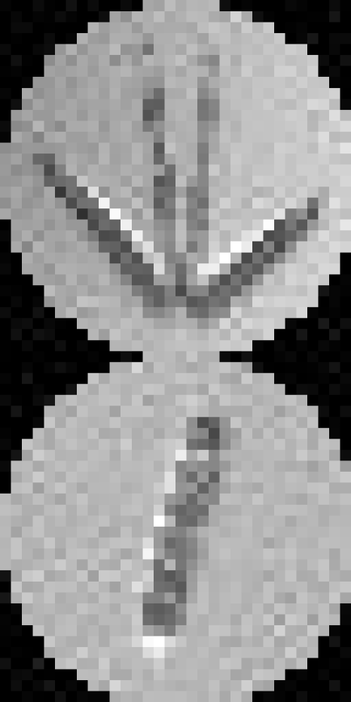
(a) Ground Truth

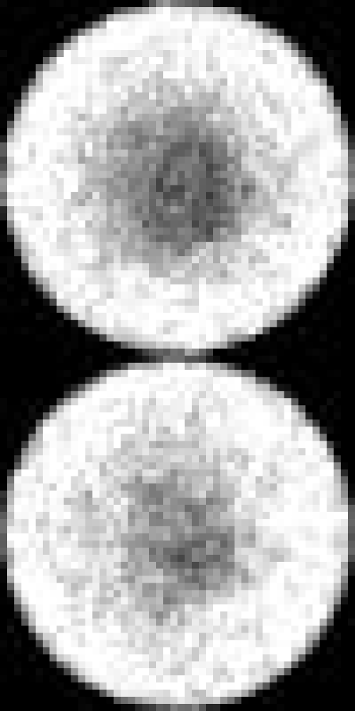
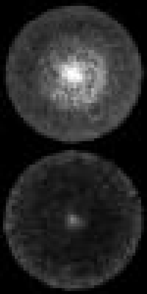
(b) TARGET-VAE

(c) IRL-INR w/o s.b.

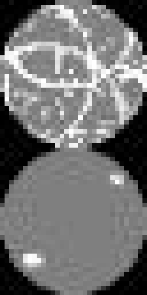
(d) IRL-INR w/ s.b.

Figure 2: Methods without symmetry fail to reconstruct WM811k and WHOI-Plankton images.

(a) MNIST (U)

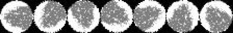
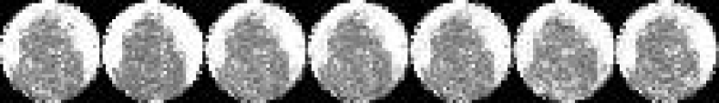
(b) WM811K

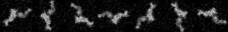
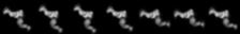
(c) 5HDB

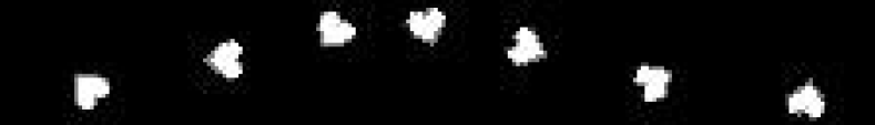
(d) dSprites

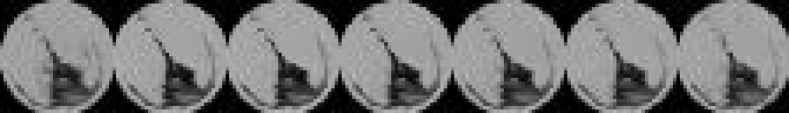
(e) WHOI-Plankton

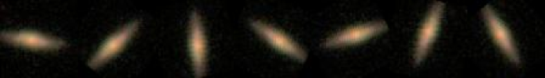
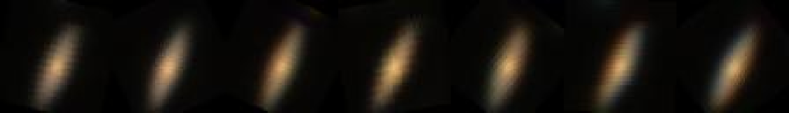
(f) Galaxy Zoo

Figure 3: To validate the disentanglement of semantic representations, we verify that the reconstructions are indeed invariant under rotation and translation. The first row of (a)–(f) are rotated by $\frac{2\pi}{7}$ degrees. The second row of (a)–(f) are reconstructions using only the semantic representation $z$, without any rotation or translation. We see that the reconstructions are invariant with respect to the rotations and translations. The setup is further detailed in Appendix F and more images are provided in Figure 12.

This canonical orientation is not orientation of the true underlying continuous image $\mathcal{I}$. The prior work of Bepler et al. (2019); Nasiri & Bepler (2022) allows the canonical orientation to be determined by the neural networks and their training process. Some of the datasets used in Nasiri & Bepler (2022) are fully rotationally symmetric (such as “MNIST(U)”) and for those setups, the symmetry makes the determination of the canonical orientation an arbitrary choice. We find that if we break the symmetry by manually prescribing a rule for the canonical orientation, the trainability of the framework significantly improves as we soon demonstrate.

We propose a symmetry breaking based on the center of mass of the image. Given a continuous image $\mathcal{I}$, we define its center of mass as

$$(m_{x},m_{y})=\frac{1}{\|\mathcal{I}\|_{1}}\int^{\infty}_{-\infty}\int^{\infty}_{-\infty}(x,y)\|\mathcal{I}(x,y)\|_{1}\;dxdy\in\mathbb{R}^{2}$$

where $\|\mathcal{I}\|_{1}=\int^{\infty}_{-\infty}\int^{\infty}_{-\infty}|\mathcal{I}(x,y)|\;dxdy$ is $L_{1}$ norm. For a discrete image $J$, we use an analogous discretized formula. Given an image $J$ with center of mass $m=(m_{x},m_{y})$, let $\tau=-m$ and let $\theta\in[0,2\pi)$ such that

$$m=\|\tau\|(\cos\theta,-\sin\theta).$$

Then $J^{\text{(can)}}=S_{\hat{\theta},\hat{\tau}}[J]$ and $J^{\text{(can)}}$ has its center of mass at $(0,0)$.

We use the symmetry-breaking loss

$$\mathcal{L}_{\text{symm}}(\phi)=\mathbb{E}_{J}[\hat{\mathcal{L}}_{\text{symm}}(J;\phi)]$$

with the per-image loss $\hat{\mathcal{L}}_{\text{symm}}(J;\phi)$ is defined as

$$(z,\hat{\tau},\hat{\theta}) =\mathbf{E}_{\phi}(J)$$

$$m =\text{CoM}(J)$$

$$\hat{\mathcal{L}}_{\text{symm}}(J;\phi) =\left\|m-\|\hat{\tau}\|(\cos\hat{\theta},-\sin\hat{\theta})\right\|^{2},$$

where $\text{CoM}(J)$ denotes the center of mass of $J$.

The use of an INR with a hypernetwork is essential in directly enforcing the representation to disentangled while allowing the network to be sufficiently expressive to be able to learn sufficiently complex tasks. Specifically, we show in Figure 2 that we could not train TARGET-VAE and IRL-INR to reconstruct the WM811k dataset without using the symmetry breaking technique.

4 Experiments

4.1 Experimental setup

The encoder network $\mathbf{E}_{\phi}(J)$ uses the ResNet18 architecture (He et al., 2016) with an MLP as the head. The hypernetwork $\mathbf{H}_{\psi}(z)$ is an MLP with input dimension $d$. The INR network $\mathbf{I}(x,y;\eta)$ uses a random Fourier feature (RFF) encoding in the style of (Rahimi & Recht, 2007; Tancik et al., 2020) followed by an MLP with output dimension 1 (for grayscale images) or 3 (for rgb images). The architectures for $\mathbf{H}_{\psi}(z)$ and $\mathbf{I}(x,y;\eta)$ are inspired by Dupont et al. (2022). Further details of the architecture can be found in Appendix A or the code provided as supplementary materials.

We use the Adam optimizer with learning rate $1\times 10^{-4}$, weight decay $5\times 10^{-4}$, and batch size $128$. For the loss function scaling coefficients, we use $\lambda_{\text{recon}}=\lambda_{\text{consis}}=1$ and $\lambda_{\text{symm}}=15$. We use the MSE and cosine similarity distances for the consistency loss for our results of Section 4.2 and Section 4.3, respectively.

We evaluate the performance of IRL-INR against the recent prior work TARGET-VAE (Nasiri & Bepler, 2022). For TARGET-VAE experiments, we mostly use the code and settings provided by the authors. We use the TARGET-VAE with $P_{16}$ and $d=32$, which Nasiri & Bepler (2022) report to perform the best for the clustering. For more complex datasets, such as WM811K or WHOI-PLANKTON, we increase the number of layers from $2$ to $6$ in their “spatial generator” network, as the authors did for the cryo-EM dataset. For the clustering experiments of Sections Section 4.3 and Section 4.4, we separate the training set and test set and evaluate the accuracy on the test set.

4.1.1 Datasets

MNIST(U) is derived from MNIST with random rotations and translations respectively sampled from $\mathrm{Uniform}([0,2\pi))$ and $\mathcal{N}(0,5^{2})$. To accommodate the translations, we embed the images into $50\times 50$ pixels as was done in (Nasiri & Bepler, 2022).

WM811k is a dataset of silicon wafer maps classified into 9 defect patterns (Wu et al., 2015). The wafer maps are circular, and the semiconductor fabrication process makes the data rotationally invariant. Because the original full dataset has a severe class imbalance, we distill the dataset into 7350 training set and 3557 test set images with reasonably balanced 9 defect classes and resize the images to $32\times 32$ pixels.

5HDB consists of 20,000 simulated projections of integrin $\alpha_{\text{IIb}}$ in complex with integrin $\beta_{3}$ (Lin et al., 2015; Bepler et al., 2019) with varying orientations. There are 16,000 training set and 4000 test set images of $40\times 40$ pixels.

dSprites consists of 2D shapes procedurally generated from 6 ground truth independent latent factors (Higgins et al., 2017). All possible combinations of these latents are present exactly once, resulting in 737,280 total images.

WHOI-Plankton is an expert-labeled image dataset for plankton (Orenstein et al., 2015). The orientation of the plankton with respect to the microscope is random, so the dataset exhibits rotation and translation invariance. However, the original dataset has a severe class imbalance, so we distill the dataset into 10 balanced classes with 1000 training set and 200 test set images. We also perform a circular crop and resize the images to $32\times 32$ pixels.

Galaxy Zoo consists of 61,578 RGB color images of galaxies from the Sloan Digital Sky Survey (Lintott et al., 2008). Each image is cropped and downsampled to $64\times 64$ pixels following common practice (Dieleman et al., 2015). We divide into 50,000 training set and 11,578 test set images.

4.2 Validating disentanglement

In this section, we validate whether the encoder network $\mathbf{E}_{\phi}(J)=(z,\hat{\theta},\hat{\tau})$ is indeed successfully trained to produce a semantic representation $z$ disentangled from the orientation of the input image $J$.

Figure 3 shows images and their reconstructions with MNIST(U), WM811k, 5HDB, dSprites, WHOI-Plankton, and Galaxy Zoo datasets. The first row of each subfigure shows images that have been rotated or translated from a given image, and we compute $\mathbf{E}_{\phi}(J)=(z,\hat{\theta},\hat{\tau})$. The second row of each figure is the reconstruction of these images by the disentangled semantic representation $z$. More specifically, the reconstructions correspond to $\mathbf{I}(x,y;\mathbf{H}_{\psi}(z))$ with $(x,y)$ not rotated or translated. (So the $(\hat{\theta},\hat{\tau})$ output by $\mathbf{E}_{\phi}(J)$ is not used.) We can see that the reconstruction is indeed (approximately) invariant regardless of the orientation of the input image $J$. For comparison, TARGET-VAE was unable to learn representations from the WM811k and WHOI-Plankton datasets, as discussed in Section 3.4.

Table 1 and Figure 4 shows how well the predicted rotation $\hat{\theta}$ and predicted translation $\hat{\tau}$ matched the true rotation $\theta$ and true translation $\tau$. Table 1 shows the Pearson correlation between the predicted rotation $\hat{\theta}$ and the true rotation $\theta$, predicted translation $\hat{\tau}$ and true translation $\tau$. We confirmed that our method has the highest correlation value. Also, in Figure 4 we plotted values of $\theta$ and $\hat{\theta}$. We can observe that most of predicted rotation degree are exactly same with true rotation. Interestingly, in the case of the WM811k, there were many cases where predicted degree and true degree are differed by $2\pi$, which is acceptable because the rotation degree is equivalent under mod $2\pi$.

	Translation	Rotation
Spatial-VAE	0.982, 0.983	0.005
$\text{TARGET-VAE P}_{4}$	0.975, 0.976	0.80
$\text{TARGET-VAE P}_{8}$	0.972, 0.971	0.859
$\text{TARGET-VAE P}_{16}$	0.974, 0.971	0.93
IRL-INR	0.999, 0.999	0.9891

Table 1: Correlation between true rotation and predicted rotation and true translation and predcited translation from MNIST(U).

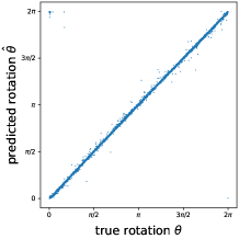
(g) MNIST(U)

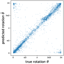
(h) WM811k

Figure 4: Difference between predicted rotation values and true rotation values on MNIST(U) and WM811.

4.3 Clustering with semantic representations and SCAN

As the semantic representations are disentangled from the orientation of the image, they should be more amenable to be used for clustering, provided that the semantic meaning of the underlying dataset is invariant under different orientations of the image. In this section, we use the semantic representations to perform clustering based on two approaches: directly with $z$ and using SCAN.

Table 2 shows the results of applying $k$-means and agglomerative clustering on the semantics representation $z$. For TARGET-VAE, we used the original authors’ code and hyperparameters to best reproduce their results. We see that the semantic representation produced by our framework IRL-INR has better clustering accuracies and has significantly less variability.

	MNIST(U)	WM811k
Spatial-VAE (K-means)	31.87 $\pm$ 3.72	27.4 $\pm$ 1.16
Spatial-VAE (Agg)	35.62 $\pm$ 2.08	28.73 $\pm$ 1.39
Target-VAE (K-means)	64.63 $\pm$ 4.4	39.6 $\pm$ 1.29
Target-VAE (Agg)	68.8 $\pm$ 4.39	40.11 $\pm$ 2.7
IRL-INR (K-means)	59.6 $\pm$ 1.12	55.06 $\pm$ 1.83
IRL-INR (Agg)	71.53 $\bf{\pm}$ 1.01	56.74 $\pm$ 1.15

Table 2: Clustering on semantics representation $z$. The confidence interval is a single standard deviation measured over 5 runs.

To further improve the clustering accuracy, we combine our framework with one of the state-of-the-art deep-learning-based method SCAN (Van Gansbeke et al., 2020). The original SCAN framework adopted SimCLR (Chen et al., 2020) as its pretext task. We instead use the training of IRL-INR as a pretext task and then use the trained encoder network $\mathbf{E}_{\phi}$ with only the $z$ output for the SCAN framework. (The $(\hat{\theta},\hat{\tau})$ are not used with SCAN.) Since SimCLR is based on InfoNCE loss (van den Oord et al., 2018), which uses cosine similarity, we also use cosine similarity distance in training IRL-INR.

Table 3 shows that IRL-INL synergizes well with SCAN to produce state-of-the-art performance. Specifically, the clustering accuracy significantly outperforms vanilla SCAN (with InfoNCE loss) and combining Target-VAE with SCAN yields little or no improvement compared to directly clustering the semantic representations of Target-VAE.

The confusion matrix Figure 5 shows that there is significant misclassification between 6 and 9. In Appendix D, we present our clustering results with the class 9 removed, and IRL-INR + SCAN achieves a 98% accuracy.

	​​​ MNIST(U)	​​​ WM811k
TARGET-VAE + SCAN	​​​ 63.09 $\pm$ 1.7	43.39 $\pm$ 4.55
SimCLR + SCAN	​​​ 85.4 $\pm$ 1.46	57.1 $\pm$ 2.81
IRL-INR + SCAN	​​​ 90.4 $\pm$ 1.74	​​​ 64.6 $\pm$ 1.01

Table 3: Using IRL-INR as pretext task for SCAN outperformed other combinations using TARGET-VAE and SimCLR. Here, $d$ is the dimension of the semantic representation $z$.

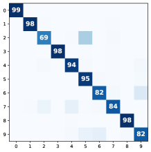
(a) MNIST(U)

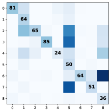
(b) WM811k

Figure 5: Confusion matrices of clustering of IRL-INR + SCAN.

4.4 Scaling latent dimension $d$

Table 4 shows that clustering accuracy of IRL-INR scales (improves) as the latent dimension $d$, the size of the semantic representation $z$, becomes larger. This phenomenon may seem counterintuitive as one might think that a smaller semantic representation is a more compressed and, therefore, better representation.

We also tried scaling the output dimension of the SimCLR + SCAN’s backbone model, but we did not find any noticeable performance gain or trend. To clarify, SimCLR + SCAN and IRL-INR + SCAN used the same backbone model, ResNet18, but only IRL-INR + SCAN exhibited the scaling improvement. We also conducted a similar scaling experiment with TARGET-VAE, but we did not find any performance gain or trend with or without SCAN.

IRL-INR + SCAN	​​​ MNIST(U)	​​​ WM811k
$d=32$	​​​ 84.18 $\pm$ 2.11	53.78 $\pm$ 3.41
$d=64$	​​​ 86 $\pm$ 1.78	​​​ 55.4 $\pm$ 1.35
$d=128$	​​​ 85.8 $\pm$ 1.46	​​​ 56.2 $\pm$ 1.16
$d=256$	​​​ 87 $\pm$ 0.89	​​​ 58.6 $\pm$ 1.62
$d=512$	​​​ 90.4 $\pm$ 1.74	​​​ 64.6 $\pm$ 1.01

Table 4: Increasing latent dimension $d$ of IRL-INR leads to better clustering performance.

4.5 Ablation studies

IRL-INR uses a hypernetwork-INR architecture, but one can alternatively consider: (1) using a simple MLP generator or (2) using a standard autoencoder while directly rotating the generated output image through pixel interpolation. We find that both alternatives fail in the following sense. For the more complex images, such as the plankton microscope or silicon wafer maps, if we use the losses for requiring the semantic representation to be invariant, then the models fail the image reconstruction pretext task in the sense that the reconstruction comes out to be a blur with no discernable content. When we nevertheless proceeded to cluster the latents, the accuracy was poor. Using the hypernetwork was the only option that allowed us to do clustering successfully for the silicon wafer maps.

Also, the loss function of IRL-INR consists of three components: (1) reconstruction loss (2) consistency loss (3) symmetry breaking loss. We conducted ablation study on the different loss terms and found that all components are essential to reconstruction and clustering. For example, removing the consistency loss does not affect the reconstruction quality but does significantly reduce the clustering accuracy. Also, as we see in Figure 2, removing the symmetry-breaking loss significantly degrades the reconstruction quality, thereby worsening the clustering results.

5 Conclusion

We proposed IRL-INR, which uses an INR with a hypernetwork to obtain semantic representations disentangled from the orientation of the image and used the semantic representations to achieve state-of-the-art clustering accuracy. Using explicit invariances in representation learning is a relatively underexplored approach. We find such representations to be especially effective in unsupervised clustering as there is a stronger reliance on inductive biases in the setup. Further exploring how to exploit various invariances exhibited in different datasets is an interesting future direction.

Appendix A Architectural details

Encoder.

For the encoder network $\mathbf{E}_{\phi}$, we use the ResNet18 architecture (He et al., 2016), a 3-layered MLP head with dimensions [512, 512, $d$+2] where $d$ is dimension of semantic representation, and the ReLU activation.

Hypernetwork.

For the Hypernetwork $\mathbf{H}_{\psi}$, we use a 4-layered MLP with dimensions [$d$, 256, 256, 256, $k$] where $k$ is the number of parameters (weights and biases) of the INR network, and the LeakyReLU(0.1) activation.

INR Network.

We parameterize a continuous image $\mathcal{I}$ by the INR-Network $\mathbf{I}$. Basically, $\mathbf{I}$ takes coordinate $(x,y)$ as an input and outputs pixel value of that coordinate. More specifically, $\mathbf{I}$ consists of two parts. For the first, $\mathbf{I}$ transforms input coordinate to fourier features following Rahimi & Recht (2007); Tancik et al. (2020), where fourier features of $(x,y)$ is defined as

$$\text{FF}(\mathbf{x})=\left(\begin{array}[]{c}\cos(2\pi B\mathbf{x})\\ \sin(2\pi B\mathbf{x})\end{array}\right)$$

with $B$ being an $f$ by $2$ random matrix whose entries are sampled from $\mathcal{N}(0,\sigma^{2})$. The number of frequencies $f$ and the variance $\sigma^{2}$ are hyperparameters. In this paper, we use $f=256$ and $\sigma=2.0$. For the second part, fourier features are fed to the 4-layered MLP with dimensions [$2f$-256-256-256-$C$], which then outputs the pixel value, where $C$ is the number of color channls ($C=1$ for greyscale images, and $C=3$ for RGB images).

Appendix B Experimental details

We report the experimental details in Table 5. We use the Adam optimizer with learning rate = 0.0001, batch size = 128, and weight decay = 0.0005, for all datasets. We train the model for 200, 500, 2000, 100 epochs for MNIST(U), WM811k, WHOI-Plankton, and {5HDB, dSprites, Galaxy zoo} respectively. We run all our experiments on a single NVIDIA RTX 3090 Ti GPU with 24 GB memory.

Dataset	LR	Batch size	WD	Epochs
MNIST(U)	0.0001	128	0.0005	200
WM811k	0.0001	128	0.0005	500
WHOI-Plankton	0.0001	512	0.001	2000
5HDB	0.0001	128	0.0005	100
dSprites	0.0001	128	0.0005	100
Galaxy Zoo	0.0001	128	0.0005	100

Table 5: Hyperparameters for the experiments

Appendix C Data-augmentation for SCAN training

The SCAN framework (Van Gansbeke et al., 2020) consists of two stages: the first stage is pretext task stage that learns a meaningful representation and the second stage is minimizing clustering loss stage. For pretext task stage, the original authors of SCAN experimented with various pretext tasks and observed that contrastive learning methods, such as MoCo (He et al., 2020) and SimCLR (Chen et al., 2020), were most effective. In this paper, we use SimCLR as the pretext task for SCAN, which the authors used for the dataset with small resolution such as CIFAR10. We denote this combination as ‘SimCLR + SCAN’.

SimCLR uses random crop (with flip and resize), color distortion and Gaussian blur data-augmentation strategies, and we denote this strategy by $\textbf{S}_{1}$. For minimizing clustering loss stage, the authors of SCAN reported that adding strong augmentations including RandAugment (Cubuk et al., 2020) and Cutout (DeVries & Taylor, 2017), which we denote by $\textbf{S}_{2}$, showed better performance. So, in the original SCAN framework, $\textbf{S}_{1}$ is applied in the first stage, and $\textbf{S}_{1}+\textbf{S}_{2}$ in the second stage.

However, if we naively follow the data-augmentation strategy used by the original SCAN, clustering performance of MNIST(U) and WM811k were suboptimal, as reported in Table 6. We suspect that this is due to the nature of contrastive learning methods. Recall that contrastive learning methods, such as SimCLR, only force the representation to be invariant under specific data augmentation strategy. Hence to extract invariant representation from dataset with strong rotation and translation variations, such as MNIST(U), WM811k, more powerful rotation and translation augmentations should be applied, especially in the pretext task stage. So we add random rotation, R, where rotation angle is sampled from $\mathrm{Uniform}([0,2\pi))$ and random translation, T, where translation is sampled from $\mathrm{Uniform}([-T,T])$. For the implementation details, we use functionals provided by Torchvision: RandomRotation(180) and RandomAffine(translate=(-T/P, T/P)) for T for R and T respectively. In our experiment, we set T = 0.07 $\times$ P where P is spatial dimension of the image.

​​​ Data Augmentation (Pretext)	​​​ Data Augmentation (Clustering)	​​​Accuracy
R​​​	R	​​​ 41.38 $\pm$ 2.07
$\textbf{R}+\textbf{T}$​​​	$\textbf{R}+\textbf{T}$	​​​ 45.19 $\pm$ 3.62
$\textbf{S}_{1}$​​​	$\textbf{S}_{1}+\textbf{S}_{2}$	​​​ 52.8 $\pm$ 3.86
$\textbf{S}_{1}+\textbf{R}$​​​	$\textbf{S}_{1}+\textbf{S}_{2}+\textbf{R}$	​​​ 83.66 $\pm$ 1.71
$\textbf{S}_{1}+\textbf{R}+\textbf{T}$​​​	$\textbf{S}_{1}+\textbf{S}_{2}+\textbf{R}+\textbf{T}$	​​​ 85.4 $\pm$ 1.46

Table 6: Data augmetation strategies for SimCLR + SCAN

For IRL-INR, we apply $\textbf{R}+\textbf{T}$ for the pretext task stage. As in the SimCLR + SCAN, IRL-INR + SCAN does benefit from stronger augmentation strategies as reported in Table 7. However, it can still outperform SimCLR + SCAN with very simple data augmentation strategies such as R, or $\textbf{R}+\textbf{T}$.

​​​ Data Augmentation (Pretext)	​​​ Data Augmentation (Clusteirng)	​​​Accuracy
$\textbf{R}+\textbf{T}$	R	​​​ 86.42 $\pm$ 1.06
$\textbf{R}+\textbf{T}$	$\textbf{R}+\textbf{T}$	​​​ 87.11 $\pm$ 1.24
$\textbf{R}+\textbf{T}$	$\textbf{S}_{1}+\textbf{S}_{2}$	​​​ 85.3 $\pm$ 1.88
$\textbf{R}+\textbf{T}$	$\textbf{S}_{1}+\textbf{S}_{2}+\textbf{R}$	​​​ 89.71 $\pm$ 2.93
$\textbf{R}+\textbf{T}$	$\textbf{S}_{1}+\textbf{S}_{2}+\textbf{R}+\textbf{T}$	​​​ 90.4 $\pm$ 1.74

Table 7: Data Augmentation Strategies for IRL-INR + SCAN

Appendix D MNIST(U)\{9}

As shown in Figure 5, clustering accuracy of MNIST(U) was low for {6} and {9}. This seems natural, because once a network has learned the rotation invariant representations of images, it could identify {6} and {9} as having similar (if not same) semantic representation.

To verify this conjecture, we experiment IRL-INR + SCAN and SimCLR + SCAN with a new dataset ’MNIST(U)\{9}’ created by removing {9} from original MNIST(U) dataset. As reported in Table 7, removing {9} significantly increased the clustering accuracy for both methods. Interestingly, by removing {9} we observed that the accuracy for {2}, which was lower than the average accuracy, significantly improved as well.

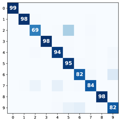
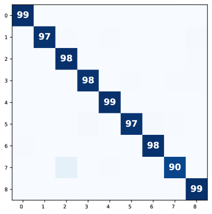
Figure 6: Confusion matrices for MNIST (U) dataset (left), and MNIST (U)\{9} dataset (right)

	​​​MNIST(U)
SimCLR + SCAN	​​​ 85.4 $\pm$ 1.46
IRL-INR + SCAN	​​​ 90.4 $\pm$ 1.74
	​​​MNIST(U)\{9}
SimCLR + SCAN	​​​ 93.8 $\pm$ 0.74
IRL-INR + SCAN	​​​ 97.6 $\pm$ 0.48

Figure 7: Clustering accuracy for MNIST(U) dataset and MNIST(U)\{9} dataset

Appendix E Reconstructing $J$

In this section, we show image samples demonstrating that the IRL-INR does faithfully reconstruct the input image $J$.

E.1 Image generation process

The encoder $\mathbf{E}_{\phi}$ outputs the rotation representation $\hat{\theta}$, translation representation $\hat{\tau}$, and semantic representation $z$. Hypernetwork $\mathbf{H}_{\psi}$ takes $z$ as an input and then outputs $\eta$, where $\eta$ is the set of weights and biases of INR network. The rotation representation $\hat{\theta}\in[0,2\pi)$ and translation representation $\hat{\tau}\in\mathbb{R}^{2}$ are trained to be estimates of the rotation and translation with respect to a certain canonical orientation. Hence, $\mathbf{I}(\tilde{x}_{p},\tilde{y}_{p};\eta)\approx J_{p}$, where $(\tilde{x}_{p},\tilde{y}_{p})=S_{\hat{\theta},\hat{\tau}}(x_{p},y_{p})$. By accurately predicting the rotation degree and translation values, IRL-INR reconstructs identical images to the input images (Figure 10).

Figure 8: Using $\hat{\theta},\hat{\tau}$ and $z$ for reconstruction $J$. The input coordinates are rotated and translated by $\hat{\theta}$ and $\hat{\tau}$ for generating $J$.

E.2 Reconstruction results for $J$

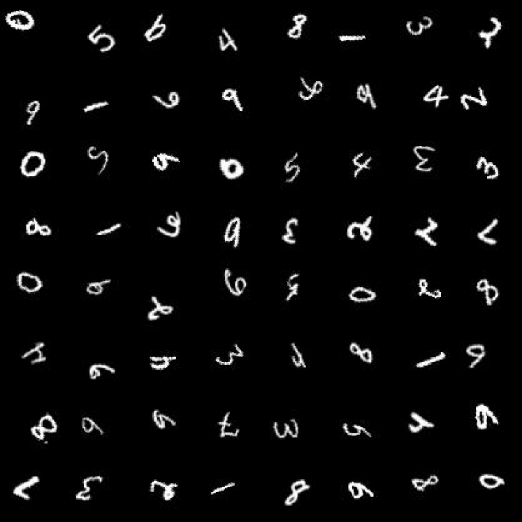
(a) Input Ground Truth

(b) Output Reconstruction

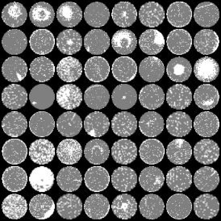
(c) Input Ground Truth

(d) Output Reconstruction

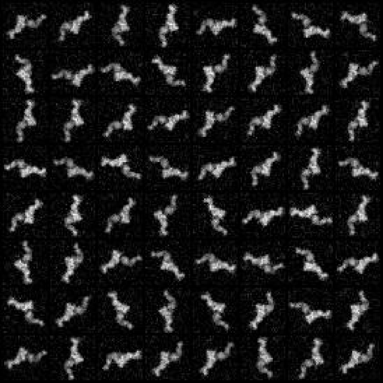
(e) Input Ground Truth

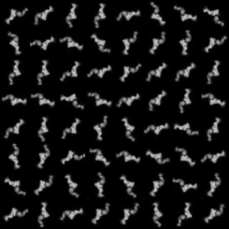
(f) Output Reconstruction

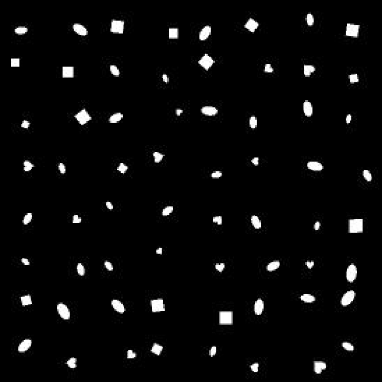
(a) Input Ground Truth

(b) Output Reconstruction

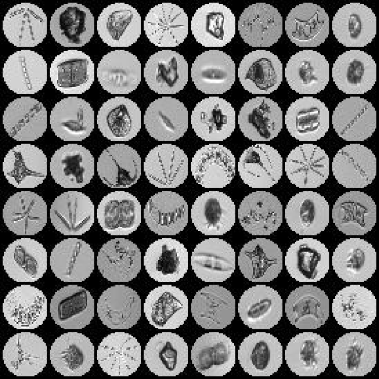
(c) Input Ground Truth

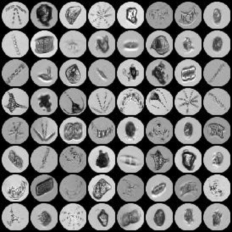
(d) Output Reconstruction

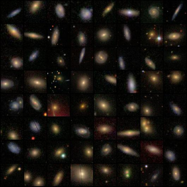
(e) Input Ground Truth

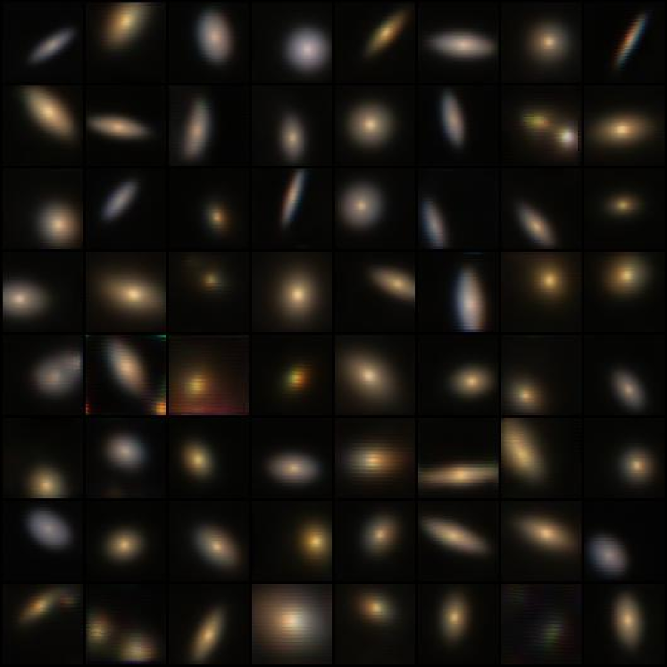
(f) Output Reconstruction

Figure 10: The output images (Right) are reconstructed very similar to the input images (Left).

Appendix F Reconstructing $J^{\text{(can)}}$

In this section, we show image samples demonstrating that IRL-INR does obtain an invariant representation of the input image $J$ regardless of its orientation. Specifically, we show that when the INR network $\mathbf{I}(\cdot,\cdot;\eta)$ is provided with non-transformed coordinates (or when $\hat{\theta},\hat{\tau}$ is ignored), the input $R_{\theta}[J]$ with any $\theta\in[0,2\pi)$ is reconstructed into the same canonical orientation $J^{\text{(can)}}$.

F.1 Image generation process

The Encoder $\mathbf{E}_{\phi}$ outputs the rotation representation $\hat{\theta}$, translation representation $\hat{\tau}$, and semantic representation $z$. Hypernetwork $\mathbf{H}_{\psi}$ takes $z$ as an input and then outputs $\eta$, where $\eta$ is the set of weights and biases of INR network. We ignore the rotation and translation representations $\hat{\theta}$ and $\hat{\tau}$, so $\mathbf{I}(x_{p},y_{p};\eta)\approx J^{\text{(can)}}_{p}$.

Figure 11: Using only $z$ for reconstruction $J^{\text{can}}$. Input NOT rotated and translated coordintates to INR network for generating $J^{\text{can}}$.

F.2 Reconstruction results for $J^{\text{can}}$

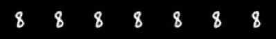
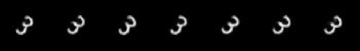
(a) MNIST(U)

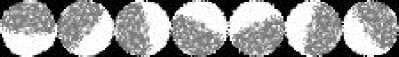
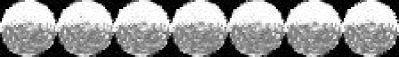
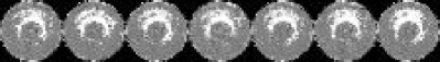
(b) WM811k

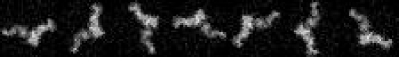
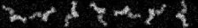
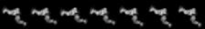
(c) 5HDB

(d) dSprites

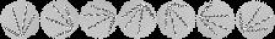
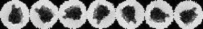
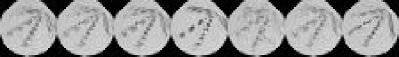
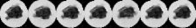
(e) WHOI-Plankton

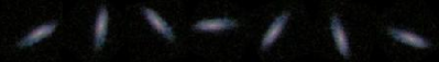
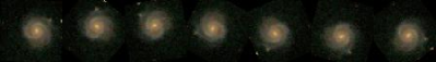
(f) Galaxy Zoo

Figure 12: To validate the disentanglement of semantic representations, we verify that the reconstructions are indeed invariant under rotation and translation. The first row of (a)–(f) are rotated by $\frac{2\pi}{7}$ degrees. The second row of (a)–(f) are reconstructions using only the semantic representation $z$, without any rotation or translation.

Appendix G Visualization of clustering results

In this section, we show image samples from each cluster to visualize the clustering performance of IRL-INR + SCAN on WM811k and MNIST(U). Each $8\times 8$ imageset in Figure 13 and 14 are sampled from same cluster.

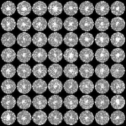
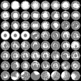
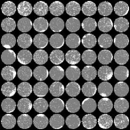
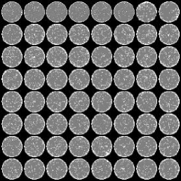
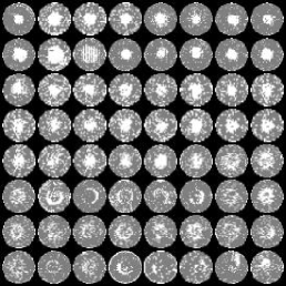
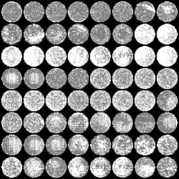
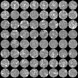
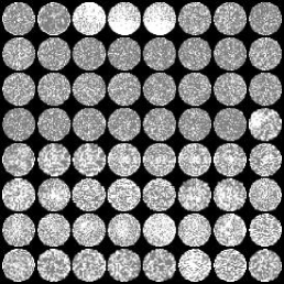
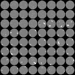
Figure 13: Visualization of WM811k clustering

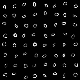
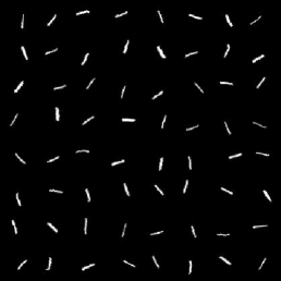
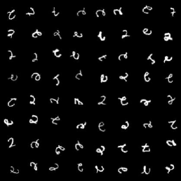
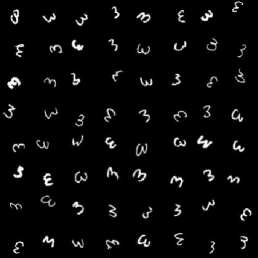
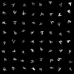
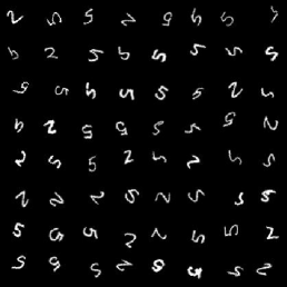
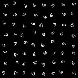
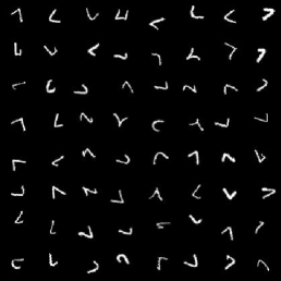
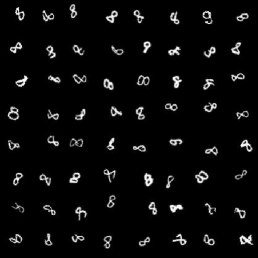
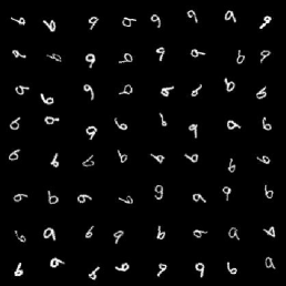
Figure 14: Visualization of MNIST(U) clustering

References

- Anokhin et al. (2020) Anokhin, I., Demochkin, K., Khakhulin, T., Sterkin, G., Lempitsky, V., and Korzhenkov, D. Image generators with conditionally-independent pixel synthesis. arXiv preprint arXiv:2011.13775, 2020.
- Bepler et al. (2019) Bepler, T., Zhong, E., Kelley, K., Brignole, E., and Berger, B. Explicitly disentangling image content from translation and rotation with spatial-VAE. Neural Information Processing Systems, 2019.
- Bromley et al. (1993) Bromley, J., Guyon, I., LeCun, Y., Säckinger, E., and Shah, R. Signature verification using a “siamese” time delay neural network. Neural Information Processing Systems, 1993.
- Chen & Salman (2011) Chen, K. and Salman, A. Extracting speaker-specific information with a regularized siamese deep network. Neural Information Processing Systems, 2011.
- Chen et al. (2018) Chen, R. T. Q., Li, X., Grosse, R. B., and Duvenaud, D. K. Isolating sources of disentanglement in variational autoencoders. Neural Information Processing Systems, 2018.
- Chen et al. (2020) Chen, T., Kornblith, S., Norouzi, M., and Hinton, G. A simple framework for contrastive learning of visual representations. International Conference on Machine Learning, 2020.
- Chen & He (2021) Chen, X. and He, K. Exploring simple siamese representation learning. Computer Vision and Pattern Recognition, 2021.
- Chen et al. (2016) Chen, X., Duan, Y., Houthooft, R., Schulman, J., Sutskever, I., and Abbeel, P. InfoGAN: Interpretable representation learning by information maximizing generative adversarial nets. Neural Information Processing Systems, 2016.
- Chen et al. (2021) Chen, Y., Liu, S., and Wang, X. Learning continuous image representation with local implicit image function. Computer Vision and Pattern Recognition, 2021.
- Comon (1994) Comon, P. Independent component analysis, a new concept? Signal Processing, 36(3):287–314, 1994.
- Cox & Hinkley (1979) Cox, D. R. and Hinkley, D. V. Theoretical Statistics. Chapman and Hall, 1979.
- Cubuk et al. (2020) Cubuk, E. D., Zoph, B., Shlens, J., and Le, Q. V. Randaugment: Practical automated data augmentation with a reduced search space. Computer Vision and Pattern Recognition Workshops, 2020.
- Dang et al. (2021) Dang, Z., Deng, C., Yang, X., Wei, K., and Huang, H. Nearest neighbor matching for deep clustering. Computer Vision and Pattern Recognition, 2021.
- Deng et al. (2021) Deng, C., Litany, O., Duan, Y., Poulenard, A., Tagliasacchi, A., and Guibas, L. J. Vector neurons: A general framework for so(3)-equivariant networks. Computer Vision and Pattern Recognition, 2021.
- DeVries & Taylor (2017) DeVries, T. and Taylor, G. W. Improved regularization of convolutional neural networks with cutout. arXiv preprint arXiv:1708.04552, 2017.
- Dieleman et al. (2015) Dieleman, S., Willett, K. W., and Dambre, J. Rotation-invariant convolutional neural networks for galaxy morphology prediction. Monthly Notices of the Royal Astronomical Society, 450(2):1441–1459, 2015.
- Dupont et al. (2022) Dupont, E., Teh, Y. W., and Doucet, A. Generative models as distributions of functions. Artificial Intelligence and Statistics, 2022.
- Dwibedi et al. (2019) Dwibedi, D., Aytar, Y., Tompson, J., Sermanet, P., and Zisserman, A. Temporal cycle-consistency learning. Computer Vision and Pattern Recognition, 2019.
- Giancola et al. (2019) Giancola, S., Zarzar, J., and Ghanem, B. Leveraging shape completion for 3d siamese tracking. Computer Vision and Pattern Recognition, 2019.
- Grill et al. (2020) Grill, J.-B., Strub, F., Altché, F., Tallec, C., Richemond, P., Buchatskaya, E., Doersch, C., Avila Pires, B., Guo, Z., Gheshlaghi Azar, M., Piot, B., kavukcuoglu, k., Munos, R., and Valko, M. Bootstrap your own latent - a new approach to self-supervised learning. Neural Information Processing Systems, 2020.
- Ha et al. (2017) Ha, D., Dai, A. M., and Le, Q. V. Hypernetworks. International Conference on Learning Representations, 2017.
- He et al. (2016) He, K., Zhang, X., Ren, S., and Sun, J. Deep residual learning for image recognition. Computer Vision and Pattern Recognition, 2016.
- He et al. (2020) He, K., Fan, H., Wu, Y., Xie, S., and Girshick, R. Momentum contrast for unsupervised visual representation learning. Computer vision and Pattern Recognition, 2020.
- Higgins et al. (2017) Higgins, I., Matthey, L., Pal, A., Burgess, C., Glorot, X., Botvinick, M., Mohamed, S., and Lerchner, A. beta-VAE: Learning basic visual concepts with a constrained variational framework. International Conference on Learning Representations, 2017.
- Hjelm et al. (2019) Hjelm, R. D., Fedorov, A., Lavoie-Marchildon, S., Grewal, K., Bachman, P., Trischler, A., and Bengio, Y. Learning deep representations by mutual information estimation and maximization. International Conference on Learning Representations, 2019.
- Hyvärinen & Oja (2000) Hyvärinen, A. and Oja, E. Independent component analysis: algorithms and applications. Neural Networks, 13(4):411–430, 2000.
- Ji et al. (2017) Ji, P., Zhang, T., Li, H., Salzmann, M., and Reid, I. Deep subspace clustering networks. Neural Information Processing Systems, 2017.
- Karras et al. (2019) Karras, T., Laine, S., and Aila, T. A style-based generator architecture for generative adversarial networks. Computer Vision and Pattern Recognition, 2019.
- Karras et al. (2021) Karras, T., Aittala, M., Laine, S., Härkönen, E., Hellsten, J., Lehtinen, J., and Aila, T. Alias-free generative adversarial networks. Neural Information Processing Systems, 2021.
- Kumar et al. (2018) Kumar, A., Sattigeri, P., and Balakrishnan, A. Variational inference of disentangled latent concepts from unlabeled observations. International Conference on Learning Representations, 2018.
- Li et al. (2021) Li, Y., Hu, P., Liu, Z., Peng, D., Zhou, J. T., and Peng, X. Contrastive clustering. American Association for Artificial Intelligence, 35(10):8547–8555, 2021.
- Lin et al. (2015) Lin, F. Y., Zhu, J., Eng, E. T., Hudson, N. E., and Springer, T. A. -subunit binding is sufficient for ligands to open the integrin headpiece. Journal of Biological Chemistry, 291(9):4537–4546, 2015.
- Lintott et al. (2008) Lintott, C. J., Schawinski, K., Slosar, A., Land, K., Bamford, S., Thomas, D., Raddick, M. J., Nichol, R. C., Szalay, A., Andreescu, D., Murray, P., and van den Berg, J. Galaxy Zoo: Morphologies derived from visual inspection of galaxies from the Sloan Digital Sky Survey. Monthly Notices of the Royal Astronomical Society, 389(3):1179–1189, 2008.
- Liu et al. (2020) Liu, Y., Neophytou, A., Sengupta, S., and Sommerlade, E. Relighting images in the wild with a self-supervised siamese auto-encoder. Winter Conference on Applications of Computer Vision, 2020.
- Locatello et al. (2020) Locatello, F., Tschannen, M., Bauer, S., Rätsch, G., Schölkopf, B., and Bachem, O. Disentangling factors of variations using few labels. International Conference on Learning Representations, 2020.
- Mildenhall et al. (2020) Mildenhall, B., Srinivasan, P. P., Tancik, M., Barron, J. T., Ramamoorthi, R., and Ng, R. Nerf: Representing scenes as neural radiance fields for view synthesis. European Conference on Computer Vision, 2020.
- Misra & Maaten (2020) Misra, I. and Maaten, L. v. d. Self-supervised learning of pretext-invariant representations. Computer Vision and Pattern Recognition, June 2020.
- Nasiri & Bepler (2022) Nasiri, A. and Bepler, T. Unsupervised object representation learning using translation and rotation group equivariant VAE. Neural Information Processing Systems, 2022.
- Orenstein et al. (2015) Orenstein, E. C., Beijbom, O., Peacock, E. E., and Sosik, H. M. WHOI-plankton- a large scale fine grained visual recognition benchmark dataset for plankton classification. arXiv:1510.00745, 2015.
- Rahimi & Recht (2007) Rahimi, A. and Recht, B. Random features for large-scale kernel machines. Neural Information Processing Systems, 2007.
- Sermanet et al. (2018) Sermanet, P., Lynch, C., Chebotar, Y., Hsu, J., Jang, E., Schaal, S., and Levine, S. Time-contrastive networks: Self-supervised learning from video. International Conference in Robotics and Automation, 2018.
- Shakunaga & Shigenari (2001) Shakunaga, T. and Shigenari, K. Decomposed eigenface for face recognition under various lighting conditions. Computer Vision and Pattern Recognition, 2001.
- Shen et al. (2021) Shen, Y., Shen, Z., Wang, M., Qin, J., Torr, P., and Shao, L. You never cluster alone. Neural Information Processing Systems, 2021.
- Shu et al. (2018) Shu, Z., Sahasrabudhe, M., Guler, R. A., Samaras, D., Paragios, N., and Kokkinos, I. Deforming autoencoders: Unsupervised disentangling of shape and appearance. European Conference on Computer Vision, 2018.
- Sitzmann et al. (2019) Sitzmann, V., Zollhöfer, M., and Wetzstein, G. Scene representation networks: Continuous 3d-structure-aware neural scene representations. Neural Information Processing Systems, 2019.
- Sitzmann et al. (2020) Sitzmann, V., Martel, J., Bergman, A., Lindell, D., and Wetzstein, G. Implicit neural representations with periodic activation functions. Neural Information Processing Systems, 2020.
- Stanley (2007) Stanley, K. O. Compositional pattern producing networks: A novel abstraction of development. Genetic Programming and Evolvable Machines, 8(2):131–162, 2007.
- Tancik et al. (2020) Tancik, M., Srinivasan, P. P., Mildenhall, B., Fridovich-Keil, S., Raghavan, N., Singhal, U., Ramamoorthi, R., Barron, J. T., and Ng, R. Fourier features let networks learn high frequency functions in low dimensional domains. Neural Information Processing Systems, 2020.
- Tian et al. (2014) Tian, F., Gao, B., Cui, Q., Chen, E., and Liu, T.-Y. Learning deep representations for graph clustering. American Association for Artificial Intelligence, 2014.
- Tran et al. (2017) Tran, L., Yin, X., and Liu, X. Disentangled representation learning GAN for pose-invariant face recognition. Computer Vision and Pattern Recognition, 2017.
- van den Oord et al. (2018) van den Oord, A., Li, Y., and Vinyals, O. Representation learning with contrastive predictive coding. arXiv:1807.03748, 2018.
- Van Gansbeke et al. (2020) Van Gansbeke, W., Vandenhende, S., Georgoulis, S., Proesmans, M., and Van Gool, L. Scan: Learning to classify images without labels. European Conference on Computer Vision, 2020.
- Wang (2008) Wang, C.-H. Recognition of semiconductor defect patterns using spatial filtering and spectral clustering. Expert Systems with Applications, 34(3):1914–1923, 2008.
- Wang & Chen (2019) Wang, R. and Chen, N. Wafer map defect pattern recognition using rotation-invariant features. IEEE Transactions on Semiconductor Manufacturing, 32(4):596–604, 2019.
- Wang & Chen (2020) Wang, R. and Chen, N. Defect pattern recognition on wafers using convolutional neural networks. Quality and Reliability Engineering International, 36(4):1245–1257, 2020.
- Wang & Gupta (2015) Wang, X. and Gupta, A. Unsupervised learning of visual representations using videos. International Conference on Computer Vision, 2015.
- Wu et al. (2015) Wu, M.-J., Jang, J.-S. R., and Chen, J. Wafer map failure pattern recognition and similarity ranking for large-scale data sets. IEEE Transactions on Semiconductor Manufacturing, 28:1–12, 2015.
- Wu et al. (2018) Wu, Z., Xiong, Y., Stella, X. Y., and Lin, D. Unsupervised feature learning via non-parametric instance discrimination. Computer Vision and Pattern Recognition, 2018.
- Xie et al. (2016) Xie, J., Girshick, R., and Farhadi, A. Unsupervised deep embedding for clustering analysis. International Conference on Machine Learning, 2016.
- Yeh et al. (2022) Yeh, C.-H., Hong, C.-Y., Hsu, Y.-C., Liu, T.-L., Chen, Y., and LeCun, Y. Decoupled contrastive learning. European Conference on Computer Vision, 2022.
- Zhang et al. (2021) Zhang, S., You, C., Vidal, R., and Li, C. Learning a self-expressive network for subspace clustering. Computer Vision and Pattern Recognition, 2021.
- Zhao et al. (2009) Zhao, F., Lin, F., and Seah, H. S. Bagging based plankton image classification. International Conference on Image Processing, 2009.
- Zhong et al. (2021) Zhong, E. D., Bepler, T., Berger, B., and Davis, J. H. CryoDRGN: Reconstruction of heterogeneous cryo-EM structures using neural networks. Nature Methods, 18(2):176–185, 2021.
- Zhou et al. (2020) Zhou, L., Chen, Y., Gao, Y., Wang, J., and Lu, H. Occlusion-aware siamese network for human pose estimation. European Conference on Computer Vision, 2020.
- Zhou et al. (2018) Zhou, P., Hou, Y., and Feng, J. Deep adversarial subspace clustering. Computer Vision and Pattern Recognition, 2018.