Constraints on the Local Cosmic Void from the Pantheon Supernovae Data

Abstract

In principle, the local cosmic void can be simply modeled by the spherically symmetric Lemaitre-Tolman-Bondi (LTB) metric. In practice, the real local cosmic void is probably not spherically symmetric. In this paper, to reconstruct a more realistic profile of the local cosmic void, we divide it into several segments. Each segment with certain solid angle is modeled by its own LTB metric. Meanwhile, we divide the 1048 type Ia supernovae (SNIa) of the Pantheon Survey into corresponding subsets according to their distribution in the galactic coordinate system. Obviously, each SNIa subset can only be used to reconstruct the profile of one segment. Finally, we can patch together an irregular profile for the local cosmic void with the whole Pantheon sample. Note that, the paucity of each data subset lead us to focus on the inner part of each void segment and assume that the half radii of the void segments are sufficient to constrain the whole segment. We find that, despite $2\sigma$ signals of anisotropy limited to the depth of the void segments, the constraints on every void segment are consistent with $\Lambda$CDM model at $95\%$ CL. Moreover, our constraints are too weak to challenge the cosmic homogeneity and isotropy.

I Introduction

The cosmological principle assumes that the universe is homogeneous and isotropic on cosmic scales. Based on this assumption as well as the standard model of particle physics and Einstein’s general relativity (GR), the Lambda cold dark matter ($\Lambda$CDM) model is proposed. This standard model of cosmology has proved successful on large cosmic scales according to the latest cosmic microwave background (CMB) observations, namely Planck 2018 data Planck:2018vyg , DES DES:2017myr or eBOSS SDSS-IV:2019txh . However, it faces major challenges on small scales, such as the Hubble tension Riess:2019cxk , the $\sigma_{8}$ tension Planck:2015lwi ; KiDS:2020ghu ; Sakr:2021jya and the dipolar tension Secrest:2020has . Besides GR, dark energy model or treatments of systematic uncertainty, the former tension also challenges the local cosmic homogeneity and the latter one challenges as well the cosmic isotropy on small scales. Therefore, further testing of the local cosmic inhomogeneity and anisotropy on small scales is necessary.

The local cosmic inhomogeneity can be modeled by the spherically symmetric Lemaitre-Tolman-Bondi (LTB) metric Lemaitre:1933gd ; Tolman:1934za ; Bondi:1947fta . Considering the late-time matter and dark energy, we can use it as an inhomogeneous generalisation of a $\Lambda$CDM model, namely as a $\Lambda$LTB model. Using the combination of the latest available cosmological observations, the local radial inhomogeneity in the $\Lambda$LTB model has been probed Camarena:2021mjr ; Camarena:2022iae . Even though a deeper local void can reconcile the Hubble tension Marra:2013rba and a larger local void can reconcile the dipolar tension Cai:2022dov , a shallower and smaller local void is favored by the combination of the latest available cosmological observations Camarena:2021mjr ; Camarena:2022iae . However, a spherically symmetric local cosmic inhomogeneity may not meet reality. Therefore, in this paper, we will probe the true profile of the local cosmic inhomogeneity as realistically as possible.

The cosmic anisotropy on small scales can be tested by type Ia supernovae (SNIa) data, such as the combined Pantheon sample Pan-STARRS1:2017jku . One straightforward method is to divide the whole samples into several subsets according to the distribution of individual SNIa in the galactic coordinate system. In particular, the hemisphere comparison method Schwarz:2007wf ; Antoniou:2010gw divides the whole sample into two data subsets which are designated as the “up” and the “down” hemispheres, respectively Deng:2018yhb ; Sun:2018cha ; Deng:2018jrp . Furthermore, $\mathsf{HEALPix}$ Gorski:2004by can be used to divide the whole sample into more data subsets Deng:2018jrp ; Andrade:2018eta ; Zhao:2013yaa . Another common method is the dipole fitting method Mariano:2012wx , which assumes a priori the existence of a dipole in the cosmic anisotropy on small scales Deng:2018yhb ; Sun:2018cha ; Deng:2018jrp ; Lin:2015rza ; Zhao:2019azy . Until now, there is no evidence for cosmic anisotropy on small scales in the SNIa samples. However, these null signals are just obtained from overall constraints and may neglect some fine structures in the universe.

In this paper, we try to test both of the local cosmic inhomogeneity and the cosmic anisotropy on small scales at the same time using the SNIa data of Pantheon. To account for the asymmetry in the local cosmic inhomogeneity and the fine structures in the cosmic anisotropy on small scales, we will fit cosmic anisotropy on small scales with the $\Lambda$LTB model. We first divide the local cosmic void into several segments. Each segment with given solid angle is fitted to its own LTB metric, where the void depth and radius parameters only correspond to the local segment and ignore the data from the other segments. We then divide the 1048 SNIa of Pantheon into corresponding subsets according to their distribution in the galactic coordinate system. Obviously, each SNIa subset can only be used to reconstruct the profile of one segment. Finally, we can patch together an irregular profile for the local cosmic void with the whole Pantheon sample. The whole profile will contain all the information about both of the local cosmic inhomogeneity and the cosmic anisotropy on small scales, as shown in Fig. 1.

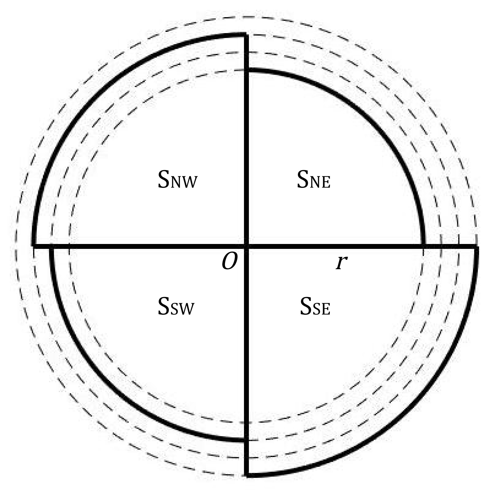
(a)

Figure 1: The diagram of an irregular local cosmic void. Each segment with the same solid angle $\pi$ is modeled by its own LTB metric and constrained by the corresponding SNIa subset given in Tab. 1. Different specific solid angle LTB segments calibrated on data from that angle allow to capture anisotropic fine structures, contrary to previous isotropic studies Camarena:2021mjr ; Camarena:2022iae . Those studies’ spherical symmetry assumption restriction might have washed away a weak signal from some fine structures. Such signal would favor the $\Lambda$LTB model over the $\Lambda$CDM model.

This paper is organized as follows. In section II, we present our method modeling the local cosmic inhomogeneity and introduce our treatment of the Pantheon data. In section III, we show the constraints on the profiles of all segments of the local cosmic inhomogeneity and compare them. Finally, a brief summary and discussions are included in section IV.

II Methodology and Data

II.1 Model

A spherically symmetric void can be modeled by the LTB metric

$$ds^{2}=-dt^{2}+\frac{R^{\prime 2}(r,t)}{1+2r^{2}k(r)\tilde{M}^{2}}dr^{2}+R^{2}(r,t)d\Omega,$$ (1)

where $d\Omega=d\theta^{2}+\sin^{2}\theta d\phi^{2}$, $\tilde{M}$ is an arbitrary mass scale, $k(r)$ is an arbitrary curvature profile function, $R(r,t)=a(t)r$ is dependent on the FLRW scale factor $a(t)$ and a prime (or dot) denotes derivative with respect to the radial coordinate $r$ (or the time $t$). As $\Lambda$CDM model is built on the FLRW metric, there is a $\Lambda$LTB model built on the LTB metric. The universe’s expansion in the $\Lambda$LTB model is determined by a Friedmann-like equation

$$\frac{\dot{R}^{2}(r,t)}{R^{2}(r,t)}=\frac{2m(r)}{R^{3}(r,t)}+\frac{2r^{2}k(r)\tilde{M}^{2}}{R^{2}(r,t)}+\frac{\Lambda}{3},$$ (2)

where $m(r)$ is the so-called Euclidean mass function and be set as $m(r)=4\pi\tilde{M}^{2}r^{3}/3$, the Big Bang time $t_{\rm BB}(r)$ is fixed as a constant and the curvature profile $k(r)$ is the only free function to determine the void. More precisely, the void’s expansion can be decomposed into a transverse expansion rate and a longitudinal expansion rate. The former one depends on a transverse scale factor $a_{\bot}(r,t)=R(r,t)/r$ as

$$H_{\bot}(r,t)= \frac{\dot{a}_{\bot}(r,t)}{a_{\bot}(r,t)};$$ (3)

while the latter one is defined by a longitudinal scale factor $a_{\parallel}(r,t)=R^{\prime}(r,t)$ as

$$H_{\parallel}(r,t)= \frac{\dot{a}_{\parallel}(r,t)}{a_{\parallel}(r,t)}.$$ (4)

According to the above Friedmann-like equation, we can define the density parameters of matter, curvature and dark energy today as

$$\Omega_{\rm m}(r)= \frac{2m(r)}{R^{3}(r,t_{0})H_{\bot}^{2}(r,t_{0})},$$ (5)

$$\Omega_{\rm k}(r)= \frac{2r^{2}k(r)\tilde{M}^{2}}{R^{2}(r,t_{0})H_{\bot}^{2}(r,t_{0})},$$ (6)

$$\Omega_{\rm\Lambda}(r)= \frac{\Lambda}{3H_{\bot}^{2}(r,t_{0})}.$$ (7)

The profile of the void can be parameterized by the depth, size, and boundary width of the void Garcia-Bellido:2008vdn . In fact, the depth and size of the void are sufficient to constrain it and the width of the void boundary can be ignored Valkenburg:2012td . We thus parameterise the void with the following curvature profile

$$k(r) =k_{\rm c}P_{3}(r),$$ (8)

$$P_{n}(r) =\left\{\begin{array}[]{lcl}1-\exp\left[\frac{-(1-r/r_{\rm B})^{n}}{r/r_{\rm B}}\right]&&0\leq r<r_{\rm B}\\ 0&&r_{\rm B}\leq r\\ \end{array}\right.,$$ (11)

where we have assumed the universe is flat outside the void, $k_{\rm c}$ is the curvature at the center and $r_{\rm B}$ is the comoving radius of the void.

If the void is spherically symmetric and all the latest cosmological observations are available, the profile at $r$ can be constrained by data from any direction or sky location. Therefore, the depth of the void and the boundary of the void in particular, where the curvature reaches $0$, can be constrained relatively well Camarena:2021mjr . If the asymmetry of the void is only probed with SNIa data, however, we find that although the depth of the void can still be constrained relatively well, this is not the case for the boundary of the void, where the curvature changes to $0$. Therefore, we introduce a scale $r_{\rm C}$ where the curvature changes by $10\%$. That is to say, we will not attempt to characterise the whole void but conservatively concentrate on the partial profile of the inner void, replacing Eq. (11) with the following function:

$$P_{n}(r)=\left\{\begin{array}[]{lcl}1-0.1\exp\left[\frac{-\left(1-r/r_{\rm C}\right)^{n}}{r/r_{\rm C}}\right]&&0\leq r<r_{\rm C}\\ 0.9\left[1-\exp\left[\frac{-\left(1-\frac{r-r_{\rm C}}{r_{\rm B}-r_{\rm C}}\right)^{n}}{\frac{r-r_{\rm C}}{r_{\rm B}-r_{\rm C}}}\right]\right]&&r_{\rm C}\leq r<r_{\rm B}\\ 0&&r_{\rm B}\leq r\\ \end{array}\right..$$ (12)

The void now is parameterized by three parameters $\{k_{\rm c},r_{\rm C},r_{\rm B}$}. All of them are derived parameters in our code. $k_{\rm c}$ is related to $\tilde{\delta}_{0}=\tilde{\delta}(r=0,t_{0})$, where the integrated mass density contrast $\tilde{\delta}(r,t_{0})$ Camarena:2021mjr is defined as

$$\tilde{\delta}(r,t_{0})=\frac{\Omega_{m}{H_{\bot}}^{2}}{\Omega_{m}^{\rm out}{H_{0}^{\rm out}}^{2}}-1,$$ (13)

where “out” denotes the corresponding FLRW quantities. Because $-1\leq\tilde{\delta}_{0}<\infty$ is not good for the convergence of the Monte Carlo Markov Chain (MCMC), we will use a new parameter

$$\delta_{0}=\left\{\begin{array}[]{lcl}\tilde{\delta}_{0}&&\tilde{\delta}_{0}\leq 0\\ \tilde{\delta}_{0}/(1+\tilde{\delta}_{0})&&\tilde{\delta}_{0}>0\\ \end{array}\right..$$ (14)

As for the two radii $\{r_{\rm B},r_{\rm C}\}$, we will relate them to their corresponding redshifts by $r_{\rm B}=r(z_{\rm B})$ and $r_{\rm C}=r(z_{\rm C})$, where $r(z)$ satisfies the geodesic equations

$$\frac{dt}{dz}= -\frac{R^{\prime}(r,t)}{(1+z)\dot{R^{\prime}}(r,t)},$$ (15)

$$\frac{dr}{dz}= -\frac{\sqrt{1+2r^{2}k(r)\tilde{M}^{2}}}{(1+z)\dot{R^{\prime}}(r,t)}.$$ (16)

As mentioned before, the information about the whole void is out of reach of SNIa data. As we probe the central part of the void with an evaluated $r_{\rm C}$ and consider the unknown boundary to be far, but not extremely far, from that limit, we therefore further relate $r_{\rm B}$ to $r_{\rm C}$ as $r_{\rm B}=2r_{\rm C}$. That is to say, we will only conservatively concentrate on the profile of the void where $z\leq z_{\rm C}$, while the profile of the void where $z_{\rm C}<z\leq z_{\rm B}$ is set by our assumption $r_{\rm B}=2r_{\rm C}$. Moreover, as $z_{\rm B}>0$ is meaningless when $\delta_{0}\sim 0$, we relate $z_{\rm B}$ to $|\delta_{0}|$ by a free parameter $|z_{\rm B}/\delta_{0}|$ which will proceed from a uniform prior distribution $|z_{\rm B}/\delta_{0}|\in[0,100]$. The remaining free parameter $\delta_{0}$ will have a uniform prior distribution $\delta_{0}\in[-0.99,0.99]$. We finally can use the dependence of SNIa’s luminosity distance on these two synthetic void parameters $\{\delta_{0},z_{\rm B}=|\delta_{0}|\times|z_{\rm B}/\delta_{0}|\}$ to probe the profile of the void, where the angular diameter distance $d_{\rm A}$ and the luminosity distance $d_{\rm L}$ are obtained from

$$d_{\rm A}(z;\delta_{0},z_{\rm B})= R(r(z),t(z);\delta_{0},z_{\rm B}),$$ (17)

$$d_{\rm L}(z;\delta_{0},z_{\rm B})= (1+z)^{2}d_{\rm A}(z;\delta_{0},z_{\rm B}).$$ (18)

.

II.2 Data

In this paper, we only use the combined Pantheon sample Pan-STARRS1:2017jku to constrain the local cosmic void. This dataset consists of 1048 SNIa in the redshift range $0.01<z<2.3$. In Fig. 2, we show the distribution of these 1048 SNIa in the galactic coordinate system $(l,b)$. To probe the asymmetry in the local cosmic inhomogeneity, we divide the full dataset into several subsets, as listed in Tab. 1. Obviously, each SNIa subset can only give the local information of the universe which can be characterized by a corresponding LTB metric. That is to say, the whole profile of the local comic void should be reconstructed with the full SNIa dataset and described by several corresponding LTB metrics. In other words, our model obtains a probe of anisotropy as illustrated in Fig. 1. There, each LTB metric being spherically symmetric, the anisotropy of our model does not proceed from individual segments but from the assembly of the various solid angle segments. The model for each segment of the final assembly is indeed spherically symmetric. Such segment’s model is obtained by considering the data from that specific solid angle to virtually be duplicated in all directions into a spherically symmetric virtual data coverage. It then can be represented by an LTB metric. We virtually proceed by restricting the obtained LTB metric within its source data solid angle. The set of such solid-angle-restricted LTB metric is then able to capture anisotropy in the composite total model, despite originating from spherically symmetric models.

Therefore, for the case when the whole data set is used (hereafter, no cut case), we have

$$\chi^{2}=\chi^{2}_{\rm P_{\rm All}};$$ (19)

for the division between North and South galactic plane subsets (one horizontal cut case), we have

$$\chi^{2}=\chi^{2}_{\rm P_{\rm N}}+\chi^{2}_{\rm P_{\rm S}};$$ (20)

for the division between East and West galactic plane subsets (one vertical cut case), we have

$$\chi^{2}=\chi^{2}_{\rm P_{\rm E}}+\chi^{2}_{\rm P_{\rm W}};$$ (21)

for the division into four quadrant using the previous subsets of the galactic plane (two cuts case), we have

$$\chi^{2}=\chi^{2}_{\rm P_{\rm NE}}+\chi^{2}_{\rm P_{\rm NW}}+\chi^{2}_{\rm P_{\rm SE}}+\chi^{2}_{\rm P_{\rm SW}}.$$ (22)

The $\chi^{2}_{s}$ for every data subset are defined with

$$\chi^{2}_{s}=\sum(\bm{m}_{{\rm B},s}^{\rm obs}-\bm{m}_{{\rm B},s}^{\rm mod})^{T}\bm{C}^{-1}_{s}(\bm{m}_{{\rm B},s}^{\rm obs}-\bm{m}_{{\rm B},s}^{\rm mod}),$$ (23)

where $\bm{C}_{s}$ is the covariance matrix of the $s$-th subset, the apparent magnitudes $\bm{m}_{{\rm B},s}^{\rm obs}$ observed by Pantheon, including contributions from stretch $x_{1}$, color $c$ and host-galaxy correction $\Delta M$. Note that the apparent magnitude $m_{{\rm B},s,i}^{\rm mod}$ for the $i$-th SNIa of the $s$-th subset in the $\Lambda$LTB model depends on two void parameters $\{\delta_{0,s},z_{{\rm B},s}\}$ and the absolute magnitude $M_{\rm B}$ as

$$m_{{\rm B},s,i}^{{\rm mod}}(z_{i};\delta_{0,s},z_{{\rm B},s},M_{{\rm B}})\\ =5\log_{10}\frac{d_{{\rm L}}(z_{i};\delta_{0,s},z_{{\rm B},s})}{1{\rm Mpc}}+25+M_{{\rm B}}.$$ (24)

Since SNIa are supposed to be standard candles, we exclude the effects of variations of $M_{\rm B}$ in each SNIa subset on the asymmetry in the local cosmic inhomogeneity. Therefore, for every division case, we use the full dataset to constrain the only nuisance parameter $M_{\rm B}$.

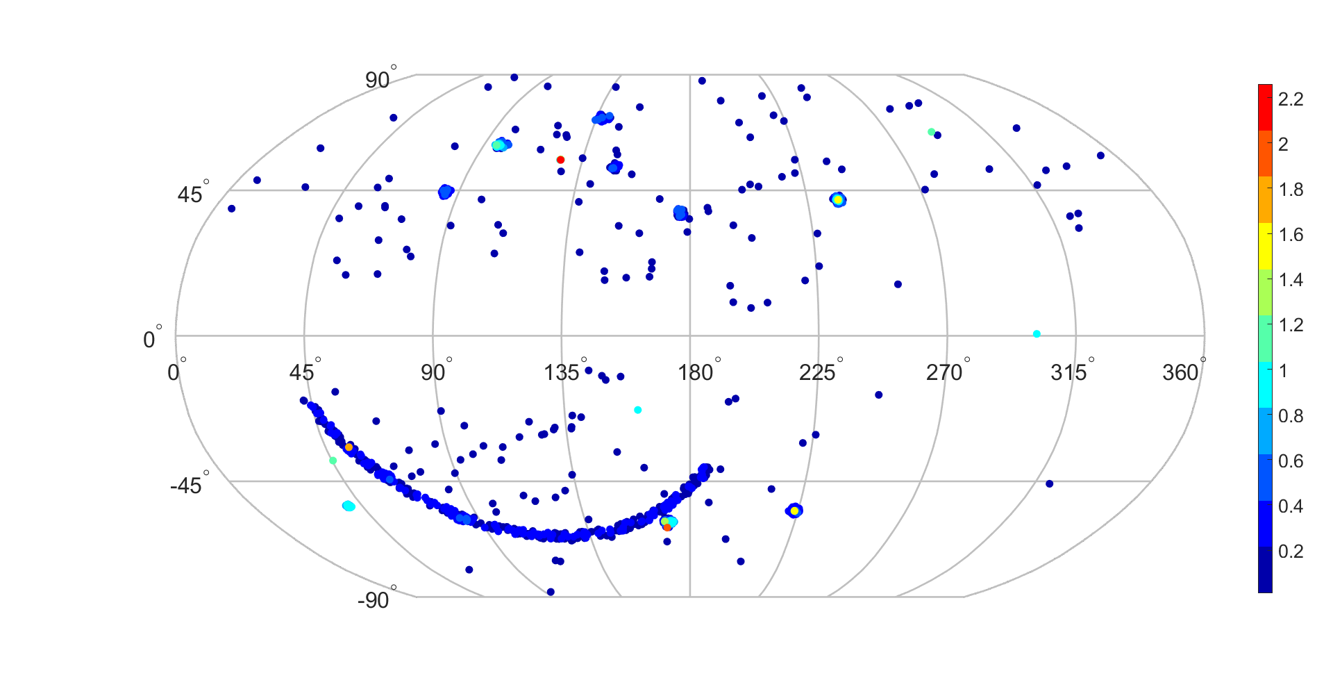
(a)

Figure 2: The distribution of 1048 SNIa of Pantheon in the galactic coordinate system $(l,b)$, where the discrete colorbar indicates the redshifts of these SNIa.

Table 1: According to the distribution of 1048 SNIa of Pantheon Pan-STARRS1:2017jku in the galactic coordinate system $(l,b)$, the full dataset is divide into $\rm P_{\rm N}$+$\rm P_{\rm S}$ by a division along the galactic plane, $\rm P_{\rm E}$+$\rm P_{\rm W}$ by a division orthogonal to the galactic plane and $\rm P_{\rm NE}$+$\rm P_{\rm NW}$+$\rm P_{\rm SE}$+$\rm P_{\rm SW}$ by both simultaneous divisions.

Dataset	$l$	$b$
$\rm P_{\rm All}$	0°$\leq l<$360°	$-90$°$\leq b\leq$90°
$\rm P_{\rm N}$	0°$\leq l<$360°	0°$\leq b\leq$90°
$\rm P_{\rm S}$	0°$\leq l<$360°	$-90$°$\leq b<$0°
$\rm P_{\rm W}$	0°$\leq l\leq$180°	$-90$°$\leq b\leq$90°
$\rm P_{\rm E}$	180°$<l<$360°	$-90$°$\leq b\leq$90°
$\rm P_{\rm NW}$	0°$\leq l\leq$180°	0°$\leq b\leq$90°
$\rm P_{\rm NE}$	180°$<l<$360°	0°$\leq b\leq$90°
$\rm P_{\rm SW}$	0°$\leq l\leq$180°	$-90$°$\leq b<$0°
$\rm P_{\rm SE}$	180°$<l<$360°	$-90$°$\leq b<$0°

III Results

The luminosity distance $d_{\rm L}(z;\delta_{0},z_{\rm B})$ in the $\Lambda$LTB model is numerically given by $\mathsf{VoidDistances2020}$ Valkenburg:2011tm which should be fed with parameters corresponding to the largest scales of the universe. The initialization of the large scale universe parameters, outside the void, is done by $\mathsf{CLASS}$ Blas:2011rf , even though we don’t use the CMB data here. For $\mathsf{CLASS}$ Blas:2011rf , we need to provide the $\Lambda$CDM model’s six parameters. In Tab. 2, we list such parameters given by Planck 2018 for TT,TE,EE+lowE+lensing Planck:2018vyg . Finally, the likelihoods in subsection II.2 are added into $\mathsf{MontePython}$ Audren:2012wb by our modified $\mathsf{monteLLTB}$ Camarena:2021mjr .

Table 2: The $\Lambda$CDM model’s six parameters given by Planck 2018 TT,TE,EE+lowE+lensing Planck:2018vyg .

$\Omega_{\rm b}h^{2}$	$\Omega_{\rm c}h^{2}$	$H_{0}[{\rm km~{}s^{-1}~{}Mpc^{-1}}]$	$\tau$	$\ln 10^{10}A_{\rm s}$	$n_{\rm s}$
$0.02237$	0.12	67.36	0.0544	3.044	0.9649

In Tab. 3, the constraints on $\{\delta_{0,s},z_{{\rm C},s},M_{\rm B}\}$ with every data subset are summarized. In Figs. 3, 4, 5 and 6, the constraints on $\{\delta_{0,s},z_{{\rm C},s},M_{\rm B}\}$ with every data subset for the no cut, horizontal cut, vertical cut and two cuts cases are also shown respectively. We choose to assume no anisotropy for $M_{B}$ and treat it as a nuisance parameter. Because we need a standard probe, we used the full data set to constrain it. This is vindicated as the results shown in Tab. 3 turn out to be self-consistent. Although we suppose $\delta_{0,s}$ of every LTB metric is only constrained with the corresponding data subset and there is no correlation between $\delta_{0,s}$, for any division case, there is an obvious correlation between $\delta_{0,s}$ in Figs. 4, 5 and 6. That correlation results from our assumption that SNIa are standard candles so all $\delta_{0,s}$ directly correlates with $M_{\rm B}$ and thus indirectly correlates with the other $\delta_{0,s}$. For every division case, the correlation between $\delta_{0,s}$ just leads to a similar error on $\delta_{0,s}$ $0.08\sim 0.10$ but imposes no effect on the mean value of $\delta_{0,s}$. Generally speaking, for all division cases, the constraints on $\delta_{0,s}$ are consistent with the FLRW metric at $95\%$ confidence level (CL): on the one hand, the constraints on $\delta_{0,s}$ are consistent with 0, which denotes cosmic homogeneity; on the other hand, the constraints on $\delta_{0,s}$ are consistent with each other, which indicates cosmic isotropy. However, the constraint on $\delta_{\rm 0,P_{SE}}=-0.15\pm 0.08$ deviates from 0 at almost $2\sigma$. This deviation results either from the paucity of data in the ${\rm P_{SE}}$ data subset or the real depth of the local cosmic void in this direction. Even though we have given up the determination of the profile at $z_{\rm C}\leq z<z_{\rm B}$ by setting $r_{\rm B}=2r_{\rm C}$, the constraints on $z_{{\rm C},s}$ are still very weak. Although we found PDF peaks at $z_{{\rm C},s}=0$ and $1\lesssim z_{{\rm C},s}\lesssim 2.26$, we can’t conclude that the Pantheon data prefers a non-zero $z_{{\rm C},s}$ to $z_{{\rm C},s}=0$.

Finally, we can use the constraints on $\{\delta_{0,s},z_{{\rm C},s}\}$ for every division case, i.e. their best fit, to probe both of the local cosmic inhomogeneity and the cosmic anisotropy on small scales. In Figs. 7, 8 and 9, we reconstruct the profile of local cosmic void $\delta(z,t_{0})$ in different direction (solid lines) with the constraints summarized in Tab. 3. At $z\lesssim z_{{\rm C},s}$ (dashed lines), the curvature changes by $10\%$. And we complete the rest of profile until $z_{{\rm B},s}$ (dotted lines) by setting $r_{\rm B}=2r_{\rm C}$. We find that even a small difference between $z_{{\rm C},s}$ can lead to a large difference between $z_{{\rm B},s}$ when the void is deeper at the center. And a deeper void (or a smaller $\delta_{0,s}$) usually favours a wider void (or a larger $z_{{\rm B},s}$). Therefore, even a smaller cosmic inhomogeneity at the center of a deeper void can lead to a larger cosmic anisotropy at the boundary of this void.

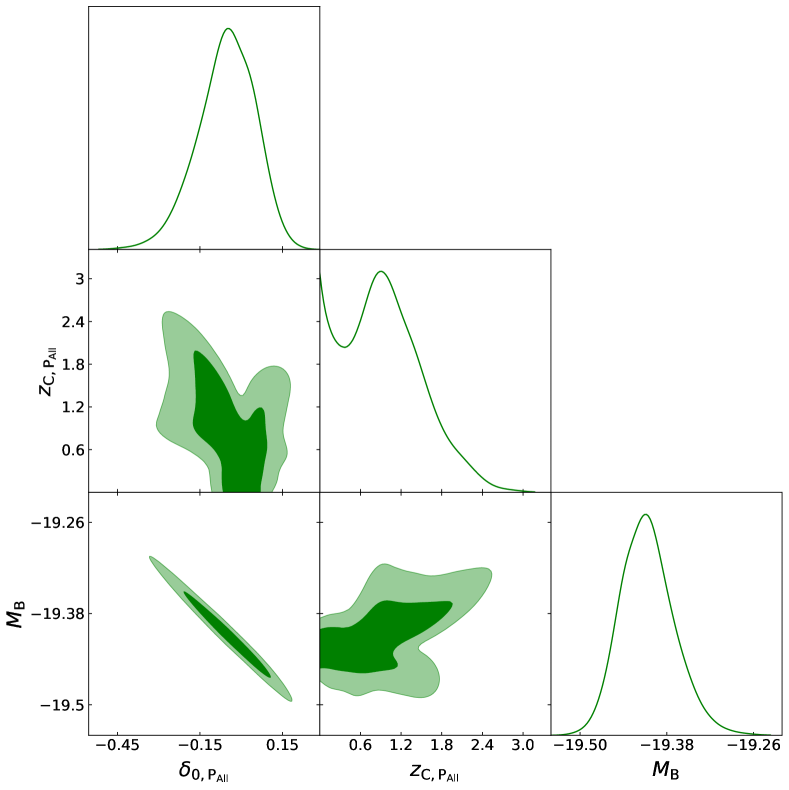
(a)

Figure 3: The triangular plot of void parameters (see Sec. III) and $M_{\rm B}$ for the no cut case, where the contours shown at $68\%$ (inner lines) and $95\%$ (outer lines) confidence ranges.

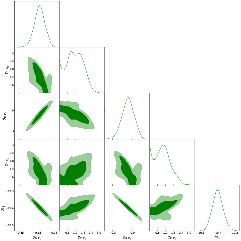
(a)

Figure 4: The triangular plot of void parameters (see Sec. III) and $M_{\rm B}$ for the horizontal cut case, where the contours shown at $68\%$ (inner lines) and $95\%$ (outer lines) confidence ranges.

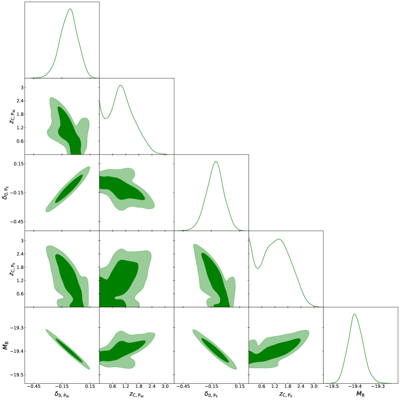
(a)

Figure 5: The triangular plot of void parameters (see Sec. III) and $M_{\rm B}$ for the vertical cut case, where the contours shown at $68\%$ (inner lines) and $95\%$ (outer lines) confidence ranges.

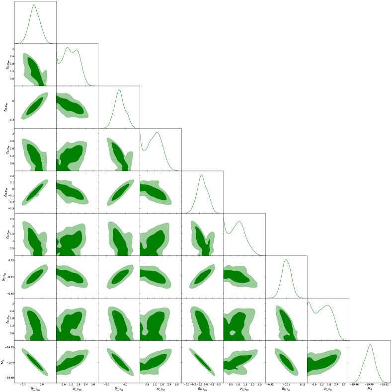
(a)

Figure 6: The triangular plot of void parameters (see Sec. III) and $M_{\rm B}$ for the two cuts case, where the contours shown at $68\%$ (inner lines) and $95\%$ (outer lines) confidence ranges.

Table 3: The constraints on void parameters (see Sec. III) and the absolute magnitude.

${\rm Dataset}$	$\delta_{0}~{}(68\%)$	$z_{{\rm C}}~{}(95\%)$	$M_{{\rm B}}~{}(68\%)$
${\rm P_{{\rm All}}}$	$-0.05\pm 0.10$	$<1.97$	$-19.41\pm 0.04$
${\rm P_{{\rm N}}}$	$-0.11\pm 0.09$	$<2.16$	$-19.40\pm 0.03$
${\rm P_{{\rm S}}}$	$-0.07\pm 0.09$	$<2.05$
${\rm P_{{\rm W}}}$	$-0.08\pm 0.09$	$<2.02$	$-19.40\pm 0.03$
${\rm P_{{\rm E}}}$	$-0.11\pm 0.09$	$<2.28$
${\rm P_{{\rm NW}}}$	$-0.11\pm 0.08$	$<2.16$	$-19.40\pm 0.03$
${\rm P_{{\rm NE}}}$	$-0.09\pm 0.09$	$<2.10$
${\rm P_{{\rm SW}}}$	$-0.06\pm 0.08$	$<1.88$
${\rm P_{{\rm SE}}}$	$-0.15\pm 0.08$	$<2.34$

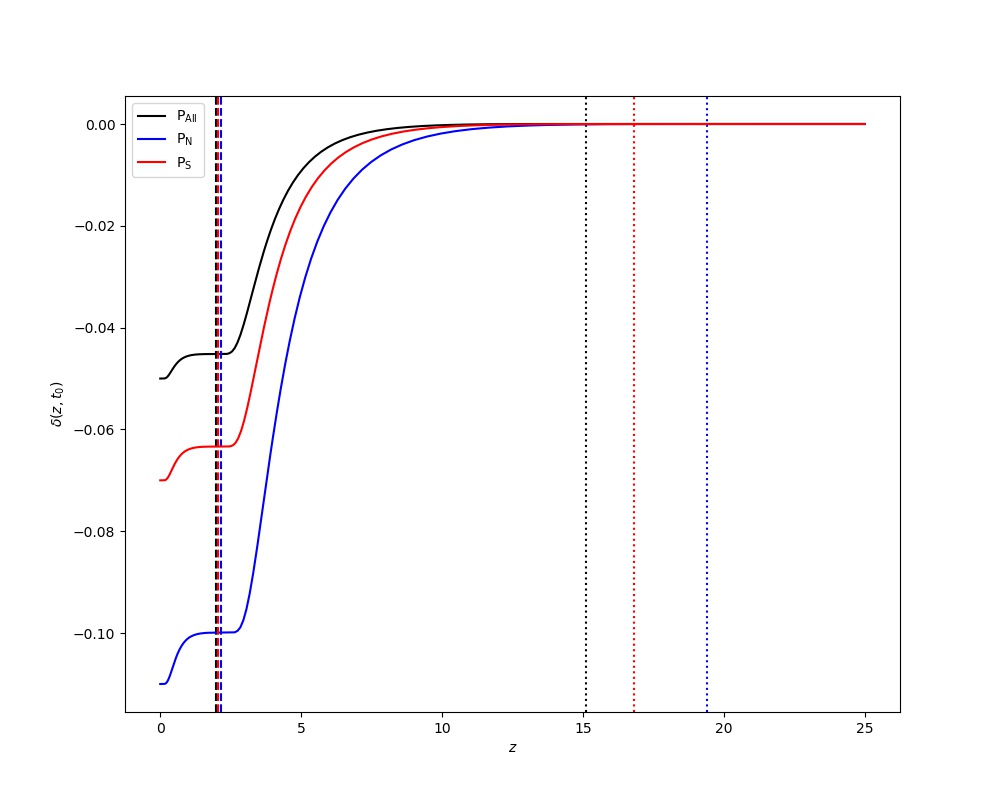
(a)

Figure 7: The integrated mass density contrast $\delta(z,t_{0})$ for the no cut and horizontal cut cases, where $\delta_{0}=-0.05$ (black solid), $z_{\rm C}=1.97$ (black dashed) and $z_{\rm B}=15.1$ (black dotted) for $\rm P_{\rm All}$, $\delta_{0}=-0.11$ (blue solid), $z_{\rm C}=2.16$ (blue dashed) and $z_{\rm B}=19.4$ (blue dotted) for $\rm P_{\rm N}$ and $\delta_{0}=-0.07$ (red solid), $z_{\rm C}=2.05$ (red dashed) and $z_{\rm B}=16.8$ (red dotted) for $\rm P_{\rm S}$ respectively.

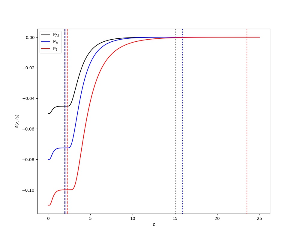
(a)

Figure 8: The integrated mass density contrast $\delta(z,t_{0})$ for the no cut and vertical cut cases, where $\delta_{0}=-0.05$ (black solid), $z_{\rm C}=1.97$ (black dashed) and $z_{\rm B}=15.1$ (black dotted) for $\rm P_{\rm All}$, $\delta_{0}=-0.08$ (blue solid), $z_{\rm C}=2.02$ (blue dashed) and $z_{\rm B}=15.9$ (blue dotted) for $\rm P_{\rm W}$ and $\delta_{0}=-0.11$ (red solid), $z_{\rm C}=2.28$ (red dashed) and $z_{\rm B}=23.5$ (red dotted) for $\rm P_{\rm E}$ respectively.

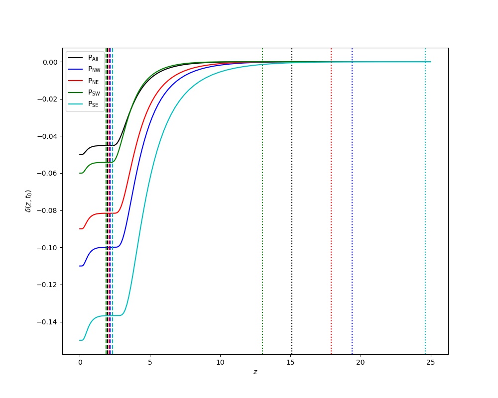
(a)

Figure 9: The integrated mass density contrast $\delta(z,t_{0})$ for the no cut and two cuts cases, where $\delta_{0}=-0.05$ (black solid), $z_{\rm C}=1.97$ (black dashed) and $z_{\rm B}=15.1$ (black dotted) for $\rm P_{\rm All}$, $\delta_{0}=-0.11$ (blue solid), $z_{\rm C}=2.16$ (blue dashed) and $z_{\rm B}=19.4$ (blue dotted) for $\rm P_{\rm NW}$, $\delta_{0}=-0.09$ (red solid), $z_{\rm C}=2.10$ (red dashed) and $z_{\rm B}=17.9$ (red dotted) for $\rm P_{\rm NE}$, $\delta_{0}=-0.06$ (green solid), $z_{\rm C}=1.88$ (green dashed) and $z_{\rm B}=13.0$ (green dotted) for $\rm P_{\rm SW}$ and $\delta_{0}=-0.15$ (cyan solid), $z_{\rm C}=2.34$ (cyan dashed) and $z_{\rm B}=24.6$ (cyan dotted) for $\rm P_{\rm SE}$ respectively.

IV Summary and Discussion

In this paper, we try to test both of the local cosmic inhomogeneity and anisotropy on small scales at the same time using the SNIa data of Pantheon. Similarly to the hemisphere comparison method, however using the LTB metric instead of the FRLW metric, we first divide the full dataset into several data subsets and then use the data subsets to constrain the void parameters $\{\delta_{0,s},z_{{\rm C},s}\}$ in the corresponding direction. Due to the paucity of data, we concentrate on the profile of the void at $z<z_{\rm C}$ where the curvature changes by $10\%$. Despite this maneuver, only $\delta_{0,s}$ turns out well constrained, contrary to $z_{{\rm C},s}$. The constraints on $\delta_{0,s}$ for all division cases are consistent with the FLRW metric at $95\%$ CL. The constraints on $z_{{\rm C},s}$ for all division cases are almost beyond $2.26$ at $95\%$ CL. That is to say, our constraints are too weak to challenge the cosmic homogeneity and isotropy. If the local cosmic void does exist, however, even a smaller cosmic inhomogeneity at the center of a deeper void can lead to a larger cosmic anisotropy at the boundary of this void.

Although our results are consistent with the cosmic homogeneity and isotropy at $95\%$ CL, as the $\delta_{0,s}$ are consistent with 0 (denoting cosmic homogeneity) while the constraints on $\delta_{0,s}$ are consistent with each other (indicating cosmic isotropy), there are some deviations from FLRW metric at $68\%$ CL. These deviations result either from the paucity of data in the subset or real physics in the corresponding direction. Therefore, more SNIa observations or other cosmological observations are needed to alleviate the possible effect of paucity of data in certain directions.

- (1) N. Aghanim et al. [Planck], “Planck 2018 results. VI. Cosmological parameters,” Astron. Astrophys. 641, A6 (2020) [erratum: Astron. Astrophys. 652, C4 (2021)] [arXiv:1807.06209 [astro-ph.CO]].
- (2) T. M. C. Abbott et al. [DES], “Dark Energy Survey year 1 results: Cosmological constraints from galaxy clustering and weak lensing,” Phys. Rev. D 98 (2018) no.4, 043526 [arXiv:1708.01530 [astro-ph.CO]].
- (3) R. Ahumada et al. [SDSS-IV], “The 16th Data Release of the Sloan Digital Sky Surveys: First Release from the APOGEE-2 Southern Survey and Full Release of eBOSS Spectra,” Astrophys. J. Suppl. 249 (2020) no.1, 3 [arXiv:1912.02905 [astro-ph.GA]].
- (4) A. G. Riess, S. Casertano, W. Yuan, L. M. Macri and D. Scolnic, “Large Magellanic Cloud Cepheid Standards Provide a 1% Foundation for the Determination of the Hubble Constant and Stronger Evidence for Physics beyond CDM,” Astrophys. J. 876, no.1, 85 (2019) [arXiv:1903.07603 [astro-ph.CO]].
- (5) P. A. R. Ade et al. [Planck], “Planck 2015 results. XXIV. Cosmology from Sunyaev-Zeldovich cluster counts,” Astron. Astrophys. 594 (2016), A24 [arXiv:1502.01597 [astro-ph.CO]].
- (6) T. Tröster et al. [KiDS], “KiDS-1000 Cosmology: Constraints beyond flat CDM,” Astron. Astrophys. 649 (2021), A88 [arXiv:2010.16416 [astro-ph.CO]].
- (7) Z. Sakr, S. Ilic and A. Blanchard, “Cluster counts - III. CDM extensions and the cluster tension,” Astron. Astrophys. 666 (2022), A34 [arXiv:2112.14171 [astro-ph.CO]].
- (8) N. J. Secrest, S. von Hausegger, M. Rameez, R. Mohayaee, S. Sarkar and J. Colin, “A Test of the Cosmological Principle with Quasars,” Astrophys. J. Lett. 908, no.2, L51 (2021) [arXiv:2009.14826 [astro-ph.CO]].
- (9) G. Lemaitre, “The expanding universe,” Annales Soc. Sci. Bruxelles A 53, 51-85 (1933)
- (10) R. C. Tolman, “Effect of imhomogeneity on cosmological models,” Proc. Nat. Acad. Sci. 20, 169-176 (1934)
- (11) H. Bondi, “Spherically symmetrical models in general relativity,” Mon. Not. Roy. Astron. Soc. 107, 410-425 (1947)
- (12) D. Camarena, V. Marra, Z. Sakr and C. Clarkson, “The Copernican principle in light of the latest cosmological data,” Mon. Not. Roy. Astron. Soc. 509, no.1, 1291-1302 (2021) [arXiv:2107.02296 [astro-ph.CO]].
- (13) D. Camarena, V. Marra, Z. Sakr and C. Clarkson, “A void in the Hubble tension? The end of the line for the Hubble bubble,” Class. Quant. Grav. 39, no.18, 184001 (2022) [arXiv:2205.05422 [astro-ph.CO]].
- (14) V. Marra, L. Amendola, I. Sawicki and W. Valkenburg, “Cosmic variance and the measurement of the local Hubble parameter,” Phys. Rev. Lett. 110, no.24, 241305 (2013) [arXiv:1303.3121 [astro-ph.CO]].
- (15) T. Cai, Q. Ding and Y. Wang, “Reconciling cosmic dipolar tensions with a gigaparsec void,” [arXiv:2211.06857 [astro-ph.CO]].
- (16) D. M. Scolnic et al. [Pan-STARRS1], “The Complete Light-curve Sample of Spectroscopically Confirmed SNe Ia from Pan-STARRS1 and Cosmological Constraints from the Combined Pantheon Sample,” Astrophys. J. 859, no.2, 101 (2018) [arXiv:1710.00845 [astro-ph.CO]]. https://vizier.cds.unistra.fr/viz-bin/VizieR-3?-source=J/ApJ/859/101/fullz
- (17) D. J. Schwarz and B. Weinhorst, “(An)isotropy of the Hubble diagram: Comparing hemispheres,” Astron. Astrophys. 474, 717-729 (2007) [arXiv:0706.0165 [astro-ph]].
- (18) I. Antoniou and L. Perivolaropoulos, “Searching for a Cosmological Preferred Axis: Union2 Data Analysis and Comparison with Other Probes,” JCAP 12, 012 (2010) [arXiv:1007.4347 [astro-ph.CO]].
- (19) H. K. Deng and H. Wei, “Testing the Cosmic Anisotropy with Supernovae Data: Hemisphere Comparison and Dipole Fitting,” Phys. Rev. D 97, no.12, 123515 (2018) [arXiv:1804.03087 [astro-ph.CO]].
- (20) Z. Q. Sun and F. Y. Wang, “Testing the anisotropy of cosmic acceleration from Pantheon supernovae sample,” Mon. Not. Roy. Astron. Soc. 478, no.4, 5153-5158 (2018) [arXiv:1805.09195 [astro-ph.CO]].
- (21) H. K. Deng and H. Wei, “Null signal for the cosmic anisotropy in the Pantheon supernovae data,” Eur. Phys. J. C 78, no.9, 755 (2018) [arXiv:1806.02773 [astro-ph.CO]].
- (22) K. M. Górski, E. Hivon, A. J. Banday, B. D. Wandelt, F. K. Hansen, M. Reinecke and M. Bartelman, “HEALPix - A Framework for high resolution discretization, and fast analysis of data distributed on the sphere,” Astrophys. J. 622, 759-771 (2005) [arXiv:astro-ph/0409513 [astro-ph]].
- (23) U. Andrade, C. A. P. Bengaly, B. Santos and J. S. Alcaniz, “A Model-independent Test of Cosmic Isotropy with Low-z Pantheon Supernovae,” Astrophys. J. 865, no.2, 119 (2018) [arXiv:1806.06990 [astro-ph.CO]].
- (24) W. Zhao, P. X. Wu and Y. Zhang, “Anisotropy of Cosmic Acceleration,” Int. J. Mod. Phys. D 22, 1350060 (2013) [arXiv:1305.2701 [astro-ph.CO]].
- (25) A. Mariano and L. Perivolaropoulos, “Is there correlation between Fine Structure and Dark Energy Cosmic Dipoles?,” Phys. Rev. D 86, 083517 (2012) [arXiv:1206.4055 [astro-ph.CO]].
- (26) H. N. Lin, S. Wang, Z. Chang and X. Li, “Testing the isotropy of the Universe by using the JLA compilation of type-Ia supernovae,” Mon. Not. Roy. Astron. Soc. 456, no.2, 1881-1885 (2016) [arXiv:1504.03428 [astro-ph.CO]].
- (27) D. Zhao, Y. Zhou and Z. Chang, “Anisotropy of the Universe via the Pantheon supernovae sample revisited,” Mon. Not. Roy. Astron. Soc. 486, no.4, 5679-5689 (2019) [arXiv:1903.12401 [astro-ph.CO]].
- (28) J. Garcia-Bellido and T. Haugboelle, “Confronting Lemaitre-Tolman-Bondi models with Observational Cosmology,” JCAP 04, 003 (2008) [arXiv:0802.1523 [astro-ph]].
- (29) W. Valkenburg, V. Marra and C. Clarkson, “Testing the Copernican principle by constraining spatial homogeneity,” Mon. Not. Roy. Astron. Soc. 438, L6-L10 (2014) [arXiv:1209.4078 [astro-ph.CO]].
- (30) W. Valkenburg, “Complete solutions to the metric of spherically collapsing dust in an expanding spacetime with a cosmological constant,” Gen. Rel. Grav. 44, 2449-2476 (2012) [arXiv:1104.1082 [gr-qc]].
- (31) D. Blas, J. Lesgourgues and T. Tram, “The Cosmic Linear Anisotropy Solving System (CLASS) II: Approximation schemes,” JCAP 07, 034 (2011) [arXiv:1104.2933 [astro-ph.CO]].
- (32) B. Audren, J. Lesgourgues, K. Benabed and S. Prunet, “Conservative Constraints on Early Cosmology: an illustration of the Monte Python cosmological parameter inference code,” JCAP 02, 001 (2013) [arXiv:1210.7183 [astro-ph.CO]].