Wenxuan Liu and Zhihai Zhang ^∗

Solving Data-Driven Newsvendor Pricing Problems with Decision-Dependent Effect

Solving Data-Driven Newsvendor Pricing Problems with Decision-Dependent Effect

Wenxuan Liu Department of Industrial Engineering, Tsinghua University, Beijing, 100084, China Zhi-Hai Zhang^∗ Department of Industrial Engineering, Tsinghua University, Beijing, 100084, China, zhzhang@tsinghua.edu.cn

This paper investigates the data-driven pricing newsvendor problem, which focuses on maximizing expected profit by deciding on inventory and pricing levels based on historical demand and feature data. We first build an approximate model by assigning weights to historical samples. However, due to decision-dependent effects, the resulting approximate model is complicated and unable to solve directly. To address this issue, we introduce the concept of approximate gradients and design an Approximate Gradient Descent (AGD) algorithm. We analyze the convergence of the proposed algorithm in both convex and non-convex settings, which correspond to the newsvendor pricing model and its variants respectively. Finally, we perform numerical experiment on both simulated and real-world dataset to demonstrate the efficiency and effectiveness of the AGD algorithm. We find that the AGD algorithm can converge to the local maximum provided that the approximation is effective. We also illustrate the significance of two characteristics: distribution-free and decision-dependent of our model. Consideration of the decision-dependent effect is necessary for approximation, and the distribution-free model is preferred when there is little information on the demand distribution and how demand reacts to the pricing decision. Moreover, the proposed model and algorithm are not limited to the newsvendor problem, but can also be used for a wide range of decision-dependent problems.

newsvendor, pricing, data-driven, prescription, approximate gradient, decision-dependent

1 Introduction

The newsvendor pricing problem plays an important role in the inventory decision theory. Nowadays, the newsvendor pricing model is applied to various fields, such as retailing, energy industry, service, and agriculture (Lin et al. 2022, Harsha et al. 2021, DeYong 2019). Compared with the traditional newsvendor model, the newsvendor pricing model has the decision-dependent property. In traditional newsvendor problems, the order decision is independent of model parameters. But in the newsvendor pricing model, the decision can affect the distribution of random parameters such as demand. We call this effect as decision-dependent effect. For example, when a charging station is to determine the electrical supply and charging price, the customers’ charging demand is influenced by its price decision. The decision-dependent effect can increase the complexity of model since the manager need to predict how the distributions change with decisions rather than predict a static distribution.

Recently, the data-driven newsvendor is also attracting attention since the demand distribution is often unknown in practice (Ban and Rudin 2018, Harsha et al. 2021). The decision maker is only accessible to the historical data. Those data often contains historical decision, random parameter and features. For instance, consider the scenario again that a charging station should determine the electricity supply and charging price in a daily frequency. First, the manager does not know the distribution of demand under specific price, but he/she is provided with the historical demand data and some feature information including date, whether and time. Those feature can also affect the distribution of random parameter. Such historical information enables the decision maker to forecast or prescribe the demand by data-driven approaches.

Our motivation stems from real-world production scenarios like assigning a new price to products. Given the inherent uncertainty of demand and the lack of information on its relationship to price, the pricing decision is challenging. This is particularly the case for the pricing of new products, where the manager only have the historical price and demand data of similar products. In this case, the manager is exactly a newsvendor and need to decide how many products to produce and how to set price for them. Another application is in the operation management of the electricity industry, where managers need to combine the historical data and today’s weather features to determine the electricity price. Because of the decision-dependent effect, the demand model consists of the demand-price relationship and the demand fluctuation. The manager can adopt the Predict-then-Optimize (PTO) framework that first predicts the demand rule by regression and then optimizes by predicted demand rule. However, if the true demand model is complex, the estimation error will be large and the subsequent optimization step will further amplify this error (Ban and Rudin 2018). Therefore, a model that integrates the prediction and optimization steps is needed. Ideally, we hope that this model will be applicable under various complex demand models and easy to solve.

The difficulty of our work lies in many aspects. The main difficulty that set our work apart from other traditional newsvendor model is the decision-dependent distribution of demand. We cannot determine the demand distribution in advance since it is affected by decisions. For this reason, we integrate the prediction and optimization steps by the prescriptive approach. But the decision variable should be assigned into the sample weight and bring nonlinearity and even non-continuity to the problem. The second barrier is the distribution-free setting. We can only use historical data to approximate the conditional demand distribution without making any assumption about the concrete form of the distribution.

In this work, we study a data-driven newsvendor pricing problem with decision-dependent property. We investigate how prescriptive methods are used to approximate the objective functions and validate the asymptotical optimality of the prescriptive approach. Because the decision-dependent approximate functions are highly nonlinear and difficult to work with, significant effort revolves around deriving an approximate gradient for the objective function. To show the validity of the approximate gradient, we analyze the convergency of the approximate gradient. Based on our approximate gradient, we develop an approximate gradient descent (AGD) algorithm in which the descent direction is determined by the approximate gradient. To validate the proposed AGD algorithm, we prove that any converge subsequences generated by AGD can converge to the points that satisfies the necessary condition for optimality. We also study the extended price-only model and price-adjustment cost model, which satisfies the convex and strongly convex conditions respectively. We show that under convex condition and certain assumptions, the objective error of AGD algorithm is bounded, indicating the theoretical guarantee when applying to our newsvendor pricing model. We further prove that the sequence of solutions provided by AGD converges to the true optimal point under the strongly convex conditions, which is in accordance with the price-adjustment cost scenario. Finally, we apply our method and algorithm to both simulated and practical datasets and confirm the effectiveness of our approach. We also demonstrate the importance of the two key properties of our model, distribution-free and decision-dependent.

1.1 Model and Approach Overview

We consider a single product scenario and the decision variables are the order quantity $q\in\mathbb{R}^{+}$ and price $p\in\mathbb{R}^{+}$. The decision maker aims to minimize its expected cost. He is provided with the historical selling information $z$ that is related to the demand $d$. Note that both the feature and the price decision can affect the distribution of demand $D\sim f_{D}(p,z)$. The company tries to minimize the expected cost, $\mathbb{E}_{D\sim f_{D}(p,z)}[l(p,q,D)]$. The true model can be represented below:

$$\min_{p,q}\mathbb{E}_{D\sim f_{D}(p,z)}[l(p,q,D)],$$ (1)

Note that the distribution of demand $f_{D}(p,z)$ is unknown. Although previous studies have proposed several widely-used demand models, for example the additive demand (Biswas and Avittathur 2018, Wang and Chen 2015) and multiplicative demand (Kazaz and Webster 2015, Salinger and Ampudia 2011) we do not make any assumption on the concrete form of $f_{D}(p,z)$. We use the feature information to link demand of the following period with historical demand data as in Bertsimas and Kallus (2019)’s work. Based on historical data, some local machine learning (ML) methods, including $k$-nearest neighbors (kNN) and kernel methods are adopted to construct the weights from data. The weights reflect the similarity between a historical sample and the present selling scenario. We construct an approximate model with such weights:

$$\min_{p,q}\mathbb{\hat{E}}_{D\sim f_{D}(p,z)}[l(p,q,D)]$$

where $\mathbb{\hat{E}}_{D\sim f_{D}(p,z)}[l(p,q,D)]$ approximates the objective function. The model is still difficult to solve because the approximate functions are nonconvex and even discontinuous if the kNN or CART weight is adopted. Therefore, we develop the approximate gradient as follows:

$$G^{N}(x;z)\overset{def}{=}\mathbb{\hat{E}}_{D\sim f_{D}(p,z)}[\nabla_{p,q}l(p,q,D)]$$

where $G^{N}(x;z)$ approximates the expectation of the objective gradient. The approximate gradient can then be used to solve the true model.

Our contributions may be summarized as follows:

1. We formally develop a data-driven approach to prescribe the distribution-free newsvendor pricing problem and extend to the price-only and price-adjustment cost scenarios. Our approach approximates the objective by weight functions generated by machine learning algorithms (nearest neighbor, kernel, tree methods). We prove the convergence performance for our approximate model. Unfortunately, the approximate model can be non-differentiable and discontinuous because of the decision-dependent effect, implying that solving the approximate model may be challenging.

2. Given the intractability of the approximate model, we develop an approximation to the gradient of true objective function, which we call the approximate gradient. The approximate gradient is derived by the same weight approximation approach as the objective functions. We prove a key consistency result of the approximate gradient function in Proposition 2.3. Namely, the approximate gradient can converge to the expectation of the profit gradient gradient under some mild conditions. The approximate gradient allows us to design gradient-based algorithms based on the approximate gradient. In our work, we develop the AGD algorithm based on the gradient descent algorithm. The concept of approximate gradient solves the difficulty when gradient information is inaccessible for the true model and the approximate model is intractable.

3. To validate our algorithm, we first prove the convergency result of AGD algorithm. We show that any converging subsequences generated by AGD algorithm converges to points that have a bounded expected gradient, which is a necessary condition of optimality (Theorem 3.3). We also investigate the convergence results for the price-only and price-adjustment cost models. We prove that the objective error is bounded under general convex conditions (Theorem 3.5), which corresponds to the price-only model without price-adjustment cost. The solution sequence generated by the algorithm converges to the true optimal solution if the strongly convex condition holds (Theorem 3.7), which corresponds to the price-adjustment cost case.

4. We gain insights from the numerical experiment on the importance of the distribution-free and decision-dependent properties in our model. Although these two properties increase the complexity of the model, ignoring the decision-dependent property will result in unreasonable predictions and solutions. At the same time, when there is a lack of information about the relationship between demand and price, the use of distribution-free model can adapt to complex unknown demand distributions.

The rest of the paper is organized as follows. Some relevant works are reviewed in Section 1.2. Section 2 outlines our approach for approximating the model and introduces the concept of approximate gradients and the approximate gradient descent algorithm. It also discusses the impact of decision-dependent effects on the resulting approximate model. In Section 3, we analyze the convergence of the AGD algorithm under non-convex, convex, and strongly convex conditions and connect these results to the newsvendor pricing model and its extended models. The experiment result on AGD algorithm with managerial insights on the distribution-free and decision-dependent properties are provided in Section 4. Section 5 concludes our work and outlines future research directions. For the briefness of reading, we furnish all the proofs in the E-companions.

1.2 Relevant Literature

In this part, we summarize some relevant streams in the literature, including newsvendor pricing problem, Distribution-free newsvendor problems and decision affects uncertainty models.

Newsvendor pricing problem. The newsvendor pricing problem has been studied for decades. A systematic review on this topic can be seen in DeYong (2019). One of the key aspect in this problem is the relationship between demand and price. There are two forms of stochastic demand: additive and multiplicative. Petruzzi and Dada (1999) gave the theoretical optimality form in both two demand scenarios. Apart from the demand uncertainty, Kazaz and Webster (2011) and Xu and Lu (2013) studied the pricing problem under uncertain supply. And Agrawal and Seshadri (2000) further investigated the risk-averse effect on the pricing decision. However, the research above relied on the assumption of a concrete demand distribution form, while we focus on distribution-free scenarios and do not impose any assumption on the form of demand distribution and its relationship to price. Harsha et al. (2021) proposed an ML framework to solve the distribution-free newsvendor pricing problem based on regression methods. But their work was limited to solving the newsvendor pricing problem. In this work, we focus on a more general framework that can solve decision-dependent problems of the same category as the newsvendor pricing problem.

There are also some variants of the newsvendor pricing problem. DeYong (2019) mentioned the price-only newsvendor model that only makes pricing decisions. The model with cost of price adjustment is another variant. In the inventory and pricing coordination literatures, the price-adjustment cost is usually employed to the multi-period inventory management problems (Lu et al. 2018, Chen et al. 2015). Although we do not consider the costs in other periods in the single-period newsvendor problems, there exists the “reference price” that plays a similar role as previous price (Chen et al. 2016, Srivastava et al. 2022). Results from Çelik et al. (2009) also showed that the change of price can affect the revenue management of perishable products. Our work investigates the extend price-only model with and without price-adjustment cost and address the nonlinearity brought by the price-adjustment cost.

Distribution-free newsvendor. Many recent studies have utilized data-driven approaches to address distribution-free newsvendor models and newsvendor pricing problems. Earlier studies estimated demand based on historical samples before solving the order decision under forecasted demand. An typical approach is the SAA. This method is to calculate the average profit under a certain decision by replacing the random variable with the demand samples (Kleywegt et al. 2002, Homem-de Mello 2001). Feng and Shanthikumar (2022) pointed out that a pure SAA approach will cause overfitting. Therefore, common approaches including adding a regularizer or constraints that can control the predicted profit variability (Levi et al. 2015, 2007, Cheung and Simchi-Levi 2019, Qin et al. 2022). The SAA approach cannot directly suit our problem because the decision variable can affect the distribution of random parameters. We cannot predict the demand by simply replacing the random parameters with historical data, since the historical decision is not equal to the decision at this moment.

The empirical risk minimization (ERM) is a promoted approach compared with the SAA method that ignores the feature information. The ERM method aims to find a function that directly maps the observed feature to optimal decision (Vapnik 1998). Ban and Rudin (2018) highlighted the importance of demand features for decision making, and they demonstrated that decision made without features is biased. They focused on the standard newsvendor model where the supply is deterministic and no risk-averse strategy is adopted, while we further consider the price decision that can affect demand. However, the ERM method cannot handle the decision-dependent property either, since it still assumes that the demand distribution is independent of price decision.

Bertsimas and Kallus (2019) proposed a general prescriptive approach to solve the prescribe optimization problem. They estimated the objective using ML methods. The input of such ML methods are features, and decision variables if the decision can affect uncertainty. The output of the ML methods are treated as the sample weight, which is used to directly estimate the true objective. We adopt the same concept of weight approximation as their work. But their work bypassed the solution approach of such model in the continuous settings, which must be addressed in our work. Bertsimas and McCord (2019) further extended the work by adding the penalize term into the objective. But they only provided solution methods on tree-based weights. And it is still not clear how to handle other types of weights. In our work, we give a general solution approach to such problems that is suitable for any kind of approximation. In Lin et al. (2022), this prescriptive model was extended to constrained conditions. They focused on the traditional newsvendor problem with profit risk constraint and contextual information. However, their work had fundamental differences with our model since they did not consider the case when decision affects uncertainty. In concrete, the supply decision would not affect the stochastic demand in traditional newsvendor problem that Lin et al. (2022) analyzed.

Other data-driven approaches related to the newsvendor problem include the quantile regression (Harsha et al. 2021), deep neural network (Pirayesh Neghab et al. 2022, Zhang 2019) and robust optimization (RO) (Xu et al. 2022). Compared with these works, we study a distribution-free pricing problem with decision-dependent effect, and extend the model to a convex price-only case and nonlinear price adjustment cost case. We manage to solve the complex decision-dependent model by proposing the concept of approximate gradient.

Decision affects uncertainty models. Though the decision-dependent effect is not fully researched in the field of data-driven management, several stochastic programming works have investigated the solution approaches to the optimization problems under this effect. Some studies addressed the problem by assuming the form of distribution. For instance, Hellemo et al. (2018) explored several ways to solve the decision-dependent models. Liu et al. (2021) developed an algorithm based on local linear regression (LLR) models. In concrete, they used LLR models to approximate the distribution in the neighborhood of a decision point. The models above relied on some assumptions on the form of the distributions. Instead, our work do not require any assumption on the distribution rule. There are also works that did not rely on the distribution assumptions. Drusvyatskiy and Xiao (2022) proposed a sampling method to solve the decision-dependent models when the distribution is under Lipschitz control. But their approach cannot be directly used in our model since we cannot access the demand distribution on every decision points, thus the sampling process cannot be carried out.

Another stream of work that considers the decision-dependent effect is the RO / distributionally robust optimization (DRO). Luo and Mehrotra (2020) constructed the decision-dependent robust set based on the distribution moment, and Xiong et al. (2021) constructed a sorting-dependent feedstock condition ambiguity set to solve a stochastic resource allocation problem. But their models relied on the knowledge of the distribution family. Noyan et al. (2021) constructed the ambiguity set by Wasserstein distance, but they assume that the distribution map is known in advance, while we treat the distribution map as an unknown function and do not impose any assumption on the form of the distribution map.

Our solution approach refers to the repeated gradient descent approaches proposed by Mendler-Dünner et al. (2020a), where the descent direction is determined through the expectation of gradient. We extend their work to the distribution-free scenario and illustrate how to approximate the expectation of gradient when the underlying distribution is unknown. Moreover, they only investigated the performance under strongly-convex condition, while we extend the performance analysis of the AGD algorithm to general cases.

In summary, this study considers several real-world costs and effects in the newsvendor pricing problem. We use the data-driven prescriptive method to construct our approximate model, but the decision-dependent effect significantly increase the complexity of approximate model and makes the gradient of the true model intractable. We develop a new approach that integrates ML approximation and stochastic programming. The solution of our model brings insights to other decision-dependent programming problems.

2 Model Description

2.1 Model and Approximation

We first construct the single-product newsvendor price-setting problem. We denote $c$ and $s$ as the purchase cost and salvage value, respectively. Given a new scenario with feature $Z=z$, the manager should determine the selling price $p$ and order quantity $q$ at the same time. We assume $s<c\leq p$, and denote the dimension of a vector $v$ as $dim(v)$. The total cost associated with the decision and random demand $D$ is:

$$l(p,q,D)=-p(D\wedge q)+cq-s(q-D)^{+}$$ (2)

where $x\wedge y=\min\{x,y\}$, and $(x)^{+}=\max\{x,0\}$.

We then substitute the cost function into model (1) and get the true newsvendor pricing model:

(True Model) $$\min_{p,q}f(p,q;z)\overset{def}{=}\mathbb{E}_{D\sim f_{D}(p,z)}[-p(D\wedge q)+cq-s(q-D)^{+}],$$ (3)

Note that the objective function in (3) is decision-dependent, which implies that the distribution $f_{D}(p,z)$ shifts correspondingly once the price decision changes.

In the data-driven problem, the distribution of $D$ is unknown for any specific $p$ and $z$ and only data $S_{N}=\{(p^{1},z^{1},D^{1}),...,(p^{N},z^{N},D^{N})\}$ is available. Let $(p^{*},q^{*})$ denotes the full-information optimal decision, which maximize the decision-dependent objective function while satisfying risk-averse constraint. The prescriptive approximation is to use $S_{N}$ to construct a data-driven approximation to (3). We approximate the model through the weighted sample approach as Bertsimas and Kallus (2019). Consider the approximate model of the form

$$\mbox{({Appr-Model})}\min_{p,q}\hat{f}(p,q;z)\overset{def}{=}\sum_{i=1}^{N}w^{i}(p,z)l(p,q,D^{i}),$$ (4)

where $w^{i}(p,z)$ are weight functions derived from the data by ML methods. Our approximate model (4) does not restrict the form of the weight functions. For briefness, we only present the definition of kNN weight below. Other definitions of weight functions (e.g. kernel regression (KR), classification and regression tree (CART), random forest (RF)) can be seen in Section 6. Readers can also refer these weight definitions to Bertsimas and Kallus (2019).

Definition 2.1 (kNN weight)

The weight function can be derived from the definition of kNN:

$$w^{\mbox{kNN},i}(p,z)=\frac{1}{k}\mathbb{I}\{(p,z)\mbox{ is a kNN of }(p^{i},z^{i})\},\quad\forall i\in[N]$$ (5)

where $\mathbb{I}\{\cdot\}$ is the indicator function, $[N]=\{1,2,...,N\}$ denotes the index set and $x^{i}$ is a kNN of $x$ if and only if $|\{j\in\{1,...,N\}\backslash i:dist(x^{j},x)<dist(x^{i},x)\}|<k$. We use the Euclidean distance $dist(x,y)=\|x-y\|_{2}$ here to represent the distance between two vectors. The kNN weight function indicates that all sample points that are among the k-nearest neighbor share the same weight, and points that are not included are not taken into consideration. Finding kNN points of $(p,z)$ can be done in $O(N*(dim(z)+1))$ time and can be sped up by using the kD tree.

We note that the weight approximation has practical meanings. It reflects the similarity between the previous condition and the current condition. The condition is variables that can affect random parameters in the model. In our newsvendor pricing problem, it means the pricing decision and features that can affect the random demands. For instance, when the distance between current condition $(p,z)$ and previous condition $(p^{i},z^{i})$ is large, the kernel weight will decrease, meaning that sample $i$ is not similar to current condition and plays a minor role in aiding the decision making.

Specifically, when we take kNN weight function, the approximate model is equivalent to a nonlinear mixed integer programming (NMIP) problem in (6). This equivalent model can exemplify the intractability incurred by the decision-dependent effect.

$$\min_{p,q,x_{i},\beta_{i},y_{i}} \sum_{i=1}^{N}x_{i}\left[-(p-c)q+(p-s)y_{i}\right]$$ (6)

s.t. $$y_{i}\geq q-D^{i},\quad\forall i\in[N]$$

$$\sum_{i=1}^{N}x_{i}=k$$

$$(p-p^{i})^{2}-(p-p^{j})^{2}+(\|z-z^{i}\|^{2}-\|z-z^{j}\|^{2})$$

$$\leq M(x_{j}-x_{i}+1),\quad\forall i\in[N],j\in[N],i\not=j$$

$$p,q\geq 0,x_{i}\in\{0,1\},y_{i}\geq 0,\quad\forall i\in[N]$$

where $x_{i}$ are auxiliary variables that indicates whether sample $i$ is a kNN of current condition $(p,z)$. $y_{i}$ is the auxiliary variable representing the max operator. $M$ is a sufficiently large positive number. Remark that the decision variable $x_{i}$ indeed reflects the decision-dependent characteristic since $x_{i}$ will degenerate to a weight parameter if the problem is not decision-dependent. We observe that the nonlinearity is mainly cost by $x_{i}$, indicating the decision-dependent characteristic significantly increases the complexity of the model.

We can see from the equivalent model that the approximate model is difficult to solve both in theory and in practice. It demonstrates that solving (4) is at least as difficult as optimizing a NMIP model, which is NP-hard. Indeed, for a fixed feature $z$, $\hat{f}(\cdot,\cdot;z)$ is nonlinear and not even continuous since the decision variable $p$ is in the kNN weight weight function. We are therefore motivated to develop a reasonable approach for solving the decision-dependent model.

2.2 Approximate Gradient

In this section, we focus on deriving a tractable method to solve the decision-dependent model. Our approximate function can be derived from the partial gradient of the cost function. Ideally, when the solution sequence moves to the direction of our approximate gradient, the generated sequence will converge to a stationary point as in the gradient descent method. When the cost function is convex, the corresponding sequence will get close to the optimal solution.

To begin with the derivation of the approximate gradient, we first derive the gradient of cost function. Note that since the cost function is not smooth but concave in $q$, we derive one of the subgradient. We use $\nabla$ to denote the gradient and $\partial$ to denote the subgradient.

$$\partial_{p,q}l(p,q,D)=\left\{\left[\begin{aligned} &-(D\wedge q)\\ &-(p-c)+(p-s)e\end{aligned}\right]:e\in\left[\mathbb{I}\{q>D\},\mathbb{I}\{q\geq D\}\right]\right\}$$ (7)

Though the denotation $\partial_{p,q}l(p,q,D)$ usually refers to the subgradient set of the cost function, to simplify the denotation, we use it to denote any elements belongs to the subgradient set in the following passage. In practice, the choice of element only affects the approximate gradient at $q=D$. We take the same approximate approach as model (4) , which we formally state in Definition 2.2.

Definition 2.2 (Approximate Gradient)

Given a feature $z$ and a decision point $(p,q)$, the approximate gradient at this point is defined as

$$G^{N}(p,q;z)\overset{def}{=}\sum_{i=1}^{N}w^{i}(p,q,z)\partial_{p,q}l(p,q,D^{i})$$ (8)

Note that in newsvendor pricing model, the approximate gradient is actually an approximation to all elements in the subgradient set. Next, we state the following proposition, which formally shows that the approximate gradient converge to the expectation of cost gradient.

Proposition 2.3

Suppose the joint distribution of $z,p,q$ is absolutely continuous and has density bounded away from 0 to $\infty$ on the support of $p,q,z$ and twice continuously differentiable. And suppose the dataset $\{p^{i},q^{i},D^{i}\}$ comes from an iid process. Then for arbitrary $z$, we have

$$\lim_{N\rightarrow+\infty}\sup_{p,q}\left\|G^{N}(p,q,z)-\mathbb{E}_{D,Q\sim f_{D}(p,z)}[\partial_{p,q}l(p,q,D)]\right\|=0$$

Proposition 2.3 shows the convergency of our approximate approach. We can then develop gradient-based algorithms by this approximate gradient. But before proceeding to the application of the approximate gradient, we should remark the difference between the following two concepts: the expectation of cost gradient and gradient of objective expectation. This two concepts are different because of the decision-dependent effect.

Proposition 2.4

Generally, the expectation of cost gradient $\mathbb{E}_{D\sim f_{D}(p,z)}[\partial_{p,q}l(p,q,D)]$ is not equal to the gradient of objective expectation $\partial_{p,q}\mathbb{E}_{D\sim f_{D}(p,z)}[l(p,q,D)]$. And $G^{N}(p,q,z)$ fails to converge to the subgradient of objective expectation.

Proposition 2.4 indicates that, unfortunately, our approximate gradient cannot converge to the true gradient of the objective function. But in the next section, we will show that (1) the stationary point of the expectation of gradient is a necessary condition for the optimal solution, and (2) if the cost function is convex or strong convex, the approximate gradient ascent method can generate solution sequence with bounded error.

Now we list the AGD algorithm in Algorithm 1. Note that the step sizes also need confirmation in order to implement AGD algorithm. We adopt the diminishing step size and Armijo step size in our work. The analysis on the selection of step size can be seen in the following section and numerical experiment.

Algorithm 1 Approximate Gradient Descent Algorithm

1:initial solution $p^{0},q^{0}$, step size $\eta^{r}$, dataset $\{p^{i},z^{i},D^{i}\}_{N}$;

2:solution $\hat{p}^{*},q^{*}$;

3:$r=0$;

4:while Stop criteria not satisfied do

5:     Calculate approximate subgradient $G^{N}(p^{r}_{N},q^{r}_{N};z)$ by (8);

6:     Calculate $(p^{r+1}_{N},q^{r+1}_{N})=\left((p^{r}_{N},q^{r}_{N})-\eta^{r}G^{N}(p^{r}_{N},q^{r}_{N};z)\right)^{+}$;

7:     $r=r+1$;

8:end while

9:return $p^{r}_{N},q^{r}_{N}$;

3 Convergence Analysis of the AGD Algorithm

In this section, we investigate the convergence of the sequence ${p^{r},q^{r}}$ generated by the AGD algorithm. Intuitively, the convergence results are similar to the typical gradient (or subgradient) methods if the number of samples is sufficient, since we have proved in Proposition 2.3 that the approximate gradient is close to the expectation of gradient. The convergence analysis is comprised of three parts. In Section 3.1, we state some denotations and prerequisite assumptions. In Section 3.2, we first prove the convergence result of AGD algorithm with both diminishing and armijo step size. This result does not require the convexity of cost function, thus can be used to solve our newsvendor pricing model (1). We also investigate the price-only and price-adjustment cost models which is convex and strongly-convex and show the error bound in both conditions in Section 3.3.

3.1 Preliminaries

We first introduce some denotations and assumptions for the following analysis. To simplify the denotation, we use $x=(p,q)$ to denote all decision variables In the following analysis. Thus the cost function becomes $l(x,D)$. The objective is to minimize $\mathbb{E}_{D\sim f_{D}(x,D)}[l(x,D)]$, where $f_{D}(x,D)$ denotes the probability density function of $D$.

We then introduce some assumptions that are used in both nonconvex and convex occasions.

[Defferentiate-integrate exchange] We assume that $l(x,D)$ is differentiable in $x$, and the gradient is bounded by an $L^{1}(D)$ function $g(D)$. That is, $\exists g\in L^{1}$, $\|\nabla_{x}l(x,D)\|\leq g(D)$ for all $x,D$.

where $L^{1}(D)$ denotes the set of functions that are integrable in $D$ almost everywhere (B.Folland 1999). Assumption 3.1 implicates that we can change the order of integration and derivation when calculating the derivative of the integral of $l(x,D)$ (see Theorem 2.27 in B.Folland (1999)). That is,

$$\nabla_{x}\int_{D}l(x,D)f_{D}(x,D)dv=\int_{D}\nabla_{x}(l(x,D)f_{D}(x,D))dv,$$

which enables us to access the derivative of objective function. This assumption is reasonable since most cost functions are integrable almost everywhere in practice. In the following text, we assume that the cost function satisfies Assumption 3.1.

We also assume that the distance between the decision-dependent distributions under different decisions can be bounded by the distance between the two decisions.

[$\epsilon$-sensitivity] We assume that the distribution map $f_{D}(\cdot,D)$ is $\epsilon$-sensitive. That is, for all $x_{1},x_{2}\in X$,

$$W_{1}(f_{D}(x_{1},D),f_{D}(x_{2},D))\leq\epsilon\|x_{1}-x_{2}\|_{2}$$ (9)

where $W_{1}$ denotes the earth mover’s distance (Rubner et al. 2000).

This assumption has been mentioned in Mendler-Dünner et al. (2020b). Intuitively, Assumption 3.1 ensures that the difference between decision-dependent distributions is not too large under different decisions. Therefore, when analyzing the gap between the approximate solution and the optimal solution, we can convert the difference between expectations under different distributions into the distance between decision variables.

3.2 Convergence Under Nonconvex Condition

In this section, we focus on the convergence result under general cases. We first establish the convergence to a stationary point of the cost gradient expectation for diminishing step size, and propose that the converging points of armijo step size have bounded gradient expectation. We then prove a necessary condition for optimality, which connects the two convergence results with the optimality property. Finally, we extend the convergence result to the non-smooth newsvendor pricing model.

We first introduce some assumptions that is used to prove the nonconvex convergence results.

[Same limited range] The value range of random parameter $D$ remains the same under any $x$. And the value range of $D$ is limited.

Assumption 3.2 can be satisfied in practical settings. We can take the union set of the value ranges of $D$ under different $x$ and assign the probability outside of the distribution $D|x$ as $0$. In practice, the demand is positive and we can often obtain a maximum demand, thus Assumption 3.2 holds. We denote the range and its volume as $\Omega$ and $S_{\Omega}$.

[Lipschitz continuous and Lipschitz gradient] The cost function $l(x,D)$ is smooth, Lipschitz continuous with Lipschitz gradient. And the probability density function (pdf) of random parameter $D$ has Lipschitz gradient. That is, for any $x,y\in X$, we have

$$\ (a)\frac{|l(x,D)-l(y,D)|}{|x-y|}\leq L_{1},\quad\forall D\in\Omega$$

$$\ (b)\frac{\|\nabla_{x}l(x,D)-\nabla_{x}l(y,D)\|}{|x-y|}\leq L_{2},\quad\forall D\in\Omega$$

$$\ (c)\frac{\|\nabla_{x}f_{D}(x,D)-\nabla_{x}f_{D}(y,D)\|}{|x-y|}\leq L_{3},\quad\forall D\in\Omega$$

Assumption 3.2 is reasonable since the value ranges of decision variables are usually bounded in practice. In the newsvendor pricing problem, the cost function $l(p,q,D)$ is also piecewise linear in $p$ and $q$ separately. We also assume that the distribution function of random parameters has a limited change rate when the decision $x$ changes.

[Bounded cost and distribution gradient] The absolute value of cost function and the gradient of the pdf of random parameter is bounded. In words, for any $x\in X$ and $D\in\Omega$, $|l(x,D)|\leq L_{4}$ and $\|\nabla_{x}f(x,D)\|\leq L_{5}$.

Assumption 3.2 can also be satisfied in practice since the cost is limit given a reasonable decision range. We also assume that the distribution change is smooth in $x$. In our newsvendor pricing model, the mild change in price decision will not cause sudden change in demand.

Now we first establish the theoretical convergence result of AGD under nonconvex and smooth conditions.

Proposition 3.1 (Convergence under diminishing step size)

Under assumptions 3.1 - 3.2, if the cost function $l(x,D)$ is twice differentiable in $x$ and the step size $\eta^{r}$ is diminishing with $\sum_{r=0}^{\infty}\eta^{r}=\infty$, the sample size $N$ is sufficiently large and the value range volume $S_{\Omega}$ is sufficiently small, then any limit point of the sequence generated by AGD algorithm is a stationary point of the cost gradient expectation.

$$\mbox{if }\lim_{N\rightarrow\infty}\lim_{r(\in\mathcal{K})\rightarrow\infty}x^{r}_{N}=\bar{x},\mbox{ then }\mathbb{E}_{D\sim f_{D}(\bar{x},D)}[\nabla_{x}l(\bar{x},D)]=0$$ (10)

Proposition 3.1 provides that the AGD algorithm converges to zero points of expected gradient. Notice that Proposition 3.1 relies on Assumptions 3.2 and 3.2, which are strong conditions and may cause the algorithm fails to provide a good convergence rate. When the constants in these assumptions, such as $\Omega,L_{4},L_{5}$ is large, the convergence will fail. Therefore, we then state the convergence result under armijo step size which require a milder condition.

Proposition 3.2 (Convergence under armijo step size)

Under Assumptions 3.1, 3.1 and 3.2(a), suppose the AGD algorithm adopts armijo step size with $\sigma$, and the sample size $N$ is sufficiently large, then any limit point $\bar{x}$ of the sequence generated by AGD algorithm has a bounded gradient expectation.

$$\mbox{if }\lim_{N\rightarrow\infty}\lim_{r(\in\mathcal{K})\rightarrow\infty}x^{r}_{N}=\bar{x},\mbox{ then }\|\mathbb{E}_{D\sim f_{D}(\bar{x},D)}[\nabla_{x}l(\bar{x},D)]\|\leq\frac{\epsilon L_{1}}{1-\sigma}$$ (11)

Unlike diminishing step, the expected gradient for armijo step is not guaranteed to converge to $0$, but its convergence can hold under a milder condition, where Assumptions 3.2 and 3.2 may not hold. We will see in Section 4.2 that the armijo step size is more useful than the diminishing step size in most practical cases.

The convergence results above are both relevant to the expected gradient. However, the expected gradient does not equal to the gradient of objective according to Proposition 2.4. In other words, the converged points are not the stationary point of objective function. So we need to further investigate the relationship between the converged point and optimal solution.

Theorem 3.3 (Necessary condition of optimality)

If $x^{*}$ is the optimal solution for a decision-dependent problem $\min_{x}\mathbb{E}_{D\sim f_{D}(x,D)}[l(x,D)]$, where $l$ is an $L_{1}$ Lipschitz function and Assumptions 3.1 and 3.1 are satisfied, then $\|\mathbb{E}_{D\sim f_{D}(x^{*},D)}[\nabla_{x}l(x^{*},D)]\|\leq L_{1}\epsilon$.

Theorem 3.3 builds connection between the AGD algorithm and optimality. It indicates that one necessary condition for optimality is that the norm of the expected gradient should not be too large. For diminishing step size, the expected gradient will be sufficiently small and thus satisfies the necessary condition. For armijo step size, we notice that the necessary bound in Theorem 3.3 is actually the upper bound when $\sigma=0$ in Proposition 3.2. Therefore, the AGD algorithm can satisfy the necessary condition of optimality.

For the newsvendor pricing problem, the convergence results are not strictly held since the cost function $l(x,D)$ is non-smooth on $q$. But we can also apply the AGD algorithm by selecting an element from the subgradient set. And we can also get a good convergence performance since the convergence results still holds when $q^{r}$ is in any side of $D$. The performance of AGD algorithm on such problem is further validated numerically in Section 4.2.

Remark 3.4 (Generality of the AGD algorithm and the convergence results)

It is important to note that the AGD algorithm and the convergence results are not limited to the newsvendor pricing problem. It can suit for other unconstrained models with decision-dependent property since we do not impose any assumption on the form of objective function or distribution. It also does not rely on the approximation approach. This versatility further motivates its use.

3.3 Convergence Under Convex Condition

In this section, we provide theoretical guarantee on the error bound of AGD algorithm when the cost function is convex and strongly convex. In the previous section, we conclude that the subsequences given by AGD algorithm satisfy the necessary condition of optimality. However, the optimality cannot be guaranteed in the general case. Therefore, we focus on the convex condition in this section. The goal of this section is, thus, to investigate the theoretical error bound and convergence to the optimal solution in the convex and strongly convex conditions. We also introduce two variants of newsvendor pricing model to connect the convergence analysis to practical scenarios. The analysis on the convex cases can be applied to the price-only model, and the results under the strongly-convex condition can be applied to the price-only model with price-adjustment cost.

We start with some definitions and assumptions. The price-only model shares the same objective function as the pricing model (3), but the order quantity $q$ is not a decision variable (Petruzzi and Dada 1999). In this case, the cost function is concave on the decision variable $p$. The price-only model can be written as

$$\min_{p}f_{p}(p;z,q)=\mathbb{E}_{D\sim f_{D}(p,z)}[l(p,q,D)]$$ (12)

The price-only model is still decision-dependent since the demand distribution is affected by the price decision. Note that solving the price-only model is also helpful for solving the pricing problem with order quantity decision. Since the manager can choose among several reasonable order quantities and decide the optimal prices respectively (DeYong 2019).

We are also interested in the price-adjustment cost in practice, which is defined by the absolute deviation to the original price $\tilde{p}$. That is,

$$\min_{p}f_{a}(p;z,q)=\mathbb{E}_{D\sim f_{D}(p,z)}[l_{a}(p,q,D)]$$ (13)

where

$$l_{a}(p,q,D)=l(p,q,D)+\gamma(p-\tilde{p})^{2}$$ (14)

We denote $\tilde{p}$ as the reference price. In our work, we adopt the quadratic form $\Delta(p;\tilde{p})=\gamma(p-\tilde{p})^{2}$ as Rotemberg (1982), Roberts (1992). But the choice of the price-adjustment function does not matter as long as the adjustment cost is convex on $p$, because our solution approach is only regard to the convexity of objective function. We also note that although both price-only model and price-only model with price-adjustment cost are single-variable problem, our algorithm and analysis can suit for multi-dimension decisions. Similar to Section 3.2, we still use the cost function $l(x,D)$ to perform the analysis.

To connect the sequence with optimal solution, we need a intermediate stable point that satisfies

$$x_{PS}=\arg\min_{x}\mathbb{E}_{D\sim f_{D}(x_{PS},D)}[l(x,D)]$$ (15)

In Mendler-Dünner et al. (2020a), the stable point serves as a fix point of the updating rule $x^{r+1}:=\arg\min_{x}\mathbb{E}_{D\sim f_{D}(x^{r},D)}[l(x,D)]$. They prove that the solution sequence will converge to $x_{PS}$ if the descent direction is the true expected gradient $\mathbb{E}_{D\sim f_{D}(x,D)}[\nabla_{x}l(x,D)]$ and the cost function $l(\cdot,D)$ is strongly convex. In our work, however, the expected gradient is unknown. We prove that our approximate gradient can also converge to the stable point under some conditions.

We derive performance bounds on convex and strongly convex cases under the following assumptions.

[Lipschitz gradient] $l(x,D)$ has $L^{c}_{1}$-Lipschitz gradient both in $x$ and $D$. In words, there exists $L^{c}_{1}$ such that

$$\|\nabla_{x}l(x_{1},D)-\nabla_{x}l(x_{2},D)\|\leq L^{c}_{1}\|x_{1}-x_{2}\|,\quad\forall x_{1},x_{2},D$$

$$\|\nabla_{x}l(x,D_{1})-\nabla_{x}l(x,D_{2})\|\leq L^{c}_{1}\|D_{1}-D_{2}\|,\quad\forall x,D_{1},D_{2}$$

[Lipschitz continuous and bounded gradient] $l(x,D)$ is $L^{c}_{3}$ Lipschitz continuous in $D$ and the gradient of $L$ is bounded. In words, there exists $L^{c}_{2},L^{c}_{3}$ such that

$$\|l(x,D_{1})-l(x,D_{2})\|\leq L^{c}_{2}\|D_{1}-D_{2}\|,\quad\forall x_{1},x_{2},D$$

$$\|\nabla_{x}l(x,D)\|\leq L^{c}_{3},\quad\forall x,D$$

Assumptions 3.3 and 3.3 can hold for both the price-only models with and without price-adjustment cost. Although there is quadratic term in the cost function with price-adjustment cost, which means Assumption 3.3 may not hold when $p$ is unconstrained. In practice, the price decision is usually within a reasonable range and thus 3.3 can be satisfied in most cases.

Based on the assumptions above mentioned, we then explore the theoretical guarantee of the convex and strongly convex cases, respectively.

Convex case: the price-only model

Theorem 3.5 states the error bound in the convex case.

Theorem 3.5 (Objective Error in Convex Case)

Suppose that Assumptions 3.1, 3.1 and 3.3 are satisfied. Denote $\lim_{N\rightarrow\infty}x^{r}_{N}=x^{r}$, and the optimal solution is $x^{*}$. If $l(x,D)$ is convex, after $k$ iterations,

$$\min_{0\leq r\leq k}\{\mathbb{E}_{D\sim f_{D}(x^{r},D)}[l(x^{r},D)]-\mathbb{E}_{D\sim f_{D}(x^{*},D)}[l(x^{*},D)]\}\leq \frac{\epsilon L^{c}_{2}\sum_{r=0}^{k}\eta^{r}\|x^{*}-x^{r}\|}{\sum_{r=0}^{k}\eta^{r}}$$

$$+\frac{\|x^{0}-x^{*}\|^{2}+(L^{c}_{3})^{2}\sum_{r=0}^{k}(\eta^{r})^{2}}{2\sum_{r=0}^{k}\eta^{r}}$$

Theorem 3.5 is a statement about the minimum distance between generated sequence $\mathbb{E}_{D\sim f_{D}(x^{r},D)}[l(x^{r},D)]$ and the optimal solution, $\mathbb{E}_{D\sim f_{D}(x^{*},D)}[l(x^{*},D)]$ when the sample size $N$ is sufficiently large. The error bound can be divided into two parts. The first term on the right-hand side is the the bound on the decision-dependent error, which is caused by the decision-dependent characteristic (see proof of Theorem 3.5). We observe that the decision-dependent error depends on the distribution distance $\epsilon$ and the Lipschitz constant $L^{c}_{2}$ that indicates the change rate of cost function to the change of random parameter. In other words, if the distance between the distribution under two different solutions is small, and the cost does not sensitive to the change of random parameter, then the decision-dependent error should not be an issue. However, when the decision-dependent distribution react sensitively to the change of price decision, or the cost change rapidly to the random demand, the decision-dependent error will be large, and Theorem 3.5 indicates that AGD algorithm may not be a good choice in such a scenario. We also note that the decision-dependent will decrease as the solution $x^{r}$ get close to the optimal solution $x^{*}$. Although we cannot guarantee that $x^{r}$ converge to $x^{*}$ in the general convex case, this term can be bounded by $D_{X}$, which denotes the maximum distance in the decision space (for example, the gap between maximal price and the cost), and the decision-dependent error turns into $\epsilon L^{c}_{2}D_{X}$ in such case.

The second term on the right-hand side is due to the internal error of the gradient descent algorithm. And the only way to decrease the internal error is iterating for more times. Since the step size $\eta^{r}$ is often decreasing and less than $1$, the internal error term will converge to zero as $k$ increases.

Theorem 3.5 can suit for both the price-only model and price-adjustment cost model, since in two cases the cost function $l(x,D)$ is concave in the decision variable $p$. This conclusion also applies to other decision dependent problems that takes the form of an expectation of a convex function. We apply the convergence result to the price-only model. Corollary 3.6 provides an upper bound on the gap between the solution sequence and the optimal value in the price-only model after $k$ iterations.

Corollary 3.6 (Convergence for price-only model)

For the price-only model, we denote $\lim_{N\rightarrow\infty}p^{r}_{N}=p^{r}$, and $p^{*}$ is the optimal pricing decision. If we adopt AGD algorithm with step size $\eta^{k}$ for $k$ iterations,

$$\min_{0\leq r\leq k}\{f_{p}(p^{r};z,q)-f_{p}(p^{*};z,q)\}\leq \frac{\epsilon\sum_{r=0}^{k}\eta^{r}|p^{*}-p^{r}|}{\sum_{r=0}^{k}\eta^{r}}$$

$$+\frac{(p^{0}-p^{*})^{2}+(D_{m}\wedge q)^{2}\sum_{r=0}^{k}(\eta^{r})^{2}}{2\sum_{r=0}^{k}\eta^{r}}$$

where $D_{m}$ is the maximum possible demand.

However, it is still not clear how the solution sequence can converge to the optimal point. Therefore, we investigate the distance to the optimal solution under strongly-convex condition.

Strongly-convex case: the price-only problem with price-adjustment cost

Similar to Mendler-Dünner et al. (2020a), we do not directly give the distance to the optimal point, but provide a distance bound to a stable point first. We state the distance bound between the solution sequence of AGD algorithm and the stable point $x_{PS}$ in Theorem 3.7.

Theorem 3.7 (Distance to stable points)

Suppose that Assumptions 3.1, 3.1 and 3.3 are satisfied, $l(x,D)$ is $\gamma$-strongly convex in $x$ and at least one stable point $x_{PS}$ exists. We denote $A=\gamma-\epsilon L_{1}^{c}$ and $B=L^{c}_{1}\sqrt{1+\epsilon^{2}}$. If $A\geq 2B\geq 0$ and we take the constant step size $\eta$ that satisfies

$$4B^{2}\eta^{2}-2A\eta+1=0$$

Then for any $\xi>0$, there exists a sample size $N_{0}$, for all $N>N_{0}$, we have the following conclusion after $k+1$ iterations,

case 1. if $1-2\eta A+2\eta^{2}B^{2}>0$, then

$$\|x^{k+1}_{N}-x_{PS}\|\leq C^{k+1}\|x^{1}_{N}-x^{*}\|+\xi\eta\frac{1-C^{k+1}}{1-C}$$ (16)

where $C=\sqrt{1-2\eta A+2\eta^{2}B^{2}}<1$.

case 2. if $1-2\eta A+2\eta^{2}B^{2}\leq 0$, then

for any $K>0$, there exists $k>K$, such that

$$\|x^{k+1}_{N}-x_{PS}\|\leq(1+\sqrt{2})\xi\eta$$ (17)

Theorem 3.7 shows the distance two the stationary point under the strongly-convex condition. In case 1, the bound can also be divided into two components: the first term is due to the initial distance between $x^{1}_{k}$ and $x_{PS}$ and the parameter $C$. Parameter $C$ is relevant to the strongly-convex parameter $\gamma$, the Lipschitz continuous parameter $L^{c}_{1}$ and the distribution distance $\epsilon$. When the degree of strong convexity is large, and the cost function and decision-dependent distribution do not react sensitively to the decision variables, then $C$ is small and the first term decreases rapidly. This result is reasonable since strong convexity can increase the converge speed and the decision-dependent effect diminishes as $L^{c}_{1}$ and $\epsilon$ decrease. The second term can be explained by the approximate error. As shown in Proposition 2.3, $\xi$ can be sufficiently small when the sample size is large. Therefore, we can reduce the second term by collecting more data.

In case 2, we prove that the distance will be become decreasing immediately when exceeding the bound $(1+\sqrt{2})\xi\eta$ until it reach the bound again. Therefore, we can prove that the distance will either decreasing or fluctuate around $(1+\sqrt{2})\xi\eta$.

Now we focus on the distance to the optimal solution. We have investigated the distance bound between solution sequence and stable point $x_{PS}$ in Theorem 3.7, so we only need to show the relationship between stable point and the optimal solution.

Lemma 3.8 (Theorem 4.3 in (Mendler-Dünner et al. 2020a))

Suppose that $l(x,D)$ is $L_{D}$-Lipschitz in $D$ and strongly convex, and the Assumption 3.1 is satisfied, then for every stable point $x_{PS}$, we have

$$\|x^{*}-x_{PS}\|\leq\frac{2L_{D}\epsilon}{\gamma}$$

Lemma 3.8 shows the distance bound between the stable point and optimal solution in the strongly-convex case. Based on this conclusion, we can now give the upper bound of optimality gap of the solution. Theorem 3.7 and Lemma 3.8 can be applied to the price-only model with price-adjustment cost, so we can also give the upper bound for the price-adjustment cost model.

Corollary 3.9 (Distance to optimal solution)

Suppose that all assumptions in Theorem 3.7 are satisfied, and $l(x,D)$ is $L_{D}$-Lipschitz in $D$, then after $k$ iterations, we have

$$\|x^{k+1}-x^{*}\|\leq\frac{2L_{D}\epsilon}{\gamma}+\max\left\{C^{k+1}\|x^{1}_{N}-x^{*}\|+\xi\eta\frac{1-C^{k+1}}{1-C},(1+\sqrt{2})\xi\eta\right\}$$

Corollary 3.10 (Solution gap of the price-adjustment cost model)

Denote $p^{*}$ as the optimal solution of the pricing problem with price-adjustment cost. Assume that $\gamma-\epsilon L^{c}_{1}\geq 2L^{c}_{1}\sqrt{1+\epsilon^{2}}$, and the step size $\eta$ is taken as Theorem 3.7. After $k$ iterations, for any $\xi>0$, there exists a sample size $N_{0}$, if $N>N_{0}$, the solution gap can be bounded by

$$|p^{k}-p^{*}|\leq\frac{2\epsilon}{\gamma}+\max\left\{C^{k+1}|p^{1}_{N}-p^{*}|+\xi\eta\frac{1-C^{k}}{1-C},(1+\sqrt{2}\xi\eta)\right\}$$

where $C=\sqrt{1-2\eta(\gamma-\epsilon L^{c}_{1})+2\eta^{2}(1+\epsilon^{2})(L^{c}_{1})^{2}}$, $L^{c}_{1}=2\gamma(p-\tilde{p})$.

In summary, when the cost function is strongly-convex, we can prove the performance bound to an intermediate stable point. Since the stable point is close to the optimal solution, we can then provide the distance bound to the optimal solution of AGD algorithm under strongly-convex case. The convergence result in Theorem 3.7 is suitable for both the price-only models with and without price-adjustment cost.

4 Experiments

In this section, we validate the convergence performance of the AGD algorithm and compare its performance with other methods. In our experiments, we use both simulated data and real data from the electricity industry to validate the effectiveness the proposed AGD algorithm. To demonstrate the importance of decision-dependent characteristic, we compare the results of our algorithm with those of models that do not consider decision-dependent effect in both real and simulated data. Finally, we compare our AGD algorithm with a prediction-then-optimize approach in simulated data, which provides evidence for the necessity of using distribution-free models in practice.

4.1 Data Description

We conduct numerical experiments on two datasets. The first dataset comes from a real-world power plant pricing scenario. This dataset describes the electricity demand and price situation in Victoria, Australia from 2015 to 2020. Factors affecting the electricity demand include temperature, solar exposure, holidays, rainfall, etc. The manager needs to decide on the electricity price on a daily frequency based on these features. The main challenge is that the manager does not know how demand changes with price under the current features. He/she can only estimate demand based on historical pricing and feature data. Noted that the intuitive inverse relationship between electricity consumption and price maybe not so clear in the dataset. In summer and winter when the electricity demand is high, power plants often control electricity demand by increasing prices, which results in a less significant inverse relationship between price and demand in the dataset. This also reflects the importance of decision-dependency in our model. The source of the real-world dataset can be seen in Section 9.1.

The second dataset comes from simulated data. We generated the demand, price and feature data from a known distribution and functional relationship. The aim is to maximize actual profits through optimal pricing and order quantity decisions. The underlying demand distribution and parameter values of this dataset can be found in Section 9.1.

4.2 Convergence Performance

In this section, we validate the convergence performance of the AGD algorithm from different aspects. We first test the convergence of the algorithm under kNN, kernel regression, decision tree (CART), and random forest (RF). The training of CART and RF is completed by the “scikit-learn” package in Python. The hyperparameters of each ML method are determined through grid search. Specifically, we manually discretize the value space of hyperparameters and select the best hyperparameters in the prediction model according to prediction performance. The iteration stops when the step size is below $10^{-5}$ or the solution exceeds the upper or lower bound. Finally, we use the Armijo principle to select the step size (for a comparison between Armijo step size and diminishing step size, see Section 9.2). All computations were carried out on Python 3.10, with an Inter i7-9750H processor which has 32.0 GB of RAM.

The performance of our algorithms can be evaluated according to two criteria: (1) convergence and (2) the change of objective value in each iteration. We first compare the convergence performance of the newsvendor pricing problem on the simulated dataset. According to Figure 2(b), we find that all four models are able to descent towards the local optimum. Among them, kernel regression and CART perform better, indicating that they have more accurate estimates of profit and gradient. Note that the priority of these two weight methods not always holds true, but depends on whether the weight method gives an accurate prediction on the model. As shown in Figure 2(b), we also find that the AGD algorithm has an relatively high converge rate. Among four weight functions, the gap of kNN, kernel regression and CART is below 5%.

Figure 1: Comparison among different weight functions of AGD algorithm for newsvendor pricing model (simulated dataset).

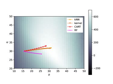
(a) Process snapshot

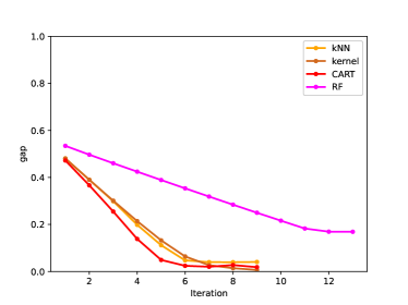
(b) Optimality gap

Secondly, we compare the convergence of the price-only model and the model considering adjustment-cost on the real-world dataset. Figure 3(b) shows the convergence results in both cases. The results show that under the price-only condition, the gap between the algorithm and the optimal value is less than 5%. We can observe that each algorithm has a slight deviation from the optimal solution before the iteration stops. This deviation reflects the approximation error of the weight approximation method. This is also why we use the Armijo rule to select the step size: the Armijo rule can ensure that the estimated function value decreases monotonically, that is, the true function value will not deviate much from the local minimum.

Figure 2: Comparison of different weight functions of AGD algorithm for price-only model with and without price-adjustment cost (real dataset).

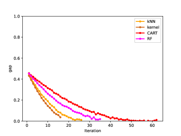
(a) Price-only model

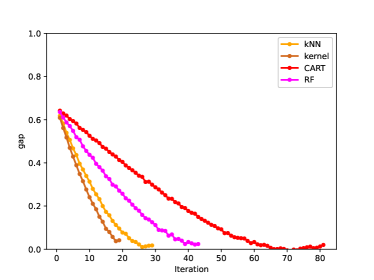
(b) Price-only model with price-adjustment cost

In order to verify the performance of the model under small sample conditions, we study the performance of the AGD algorithm under different sample sizes on the simulated dataset. We use kNN weight method with $k=20$ and generate $5$ stochastic features for each sample size. The average, maximum and minimum optimality gaps are shown in Figure 3. As expected, AGD algorithm can converges to stationary point of the true objective with small sample size. When the sample size is large, the optimality gap becomes more stable and decreases correspondingly, since a larger sample size provide more information of the true distribution.

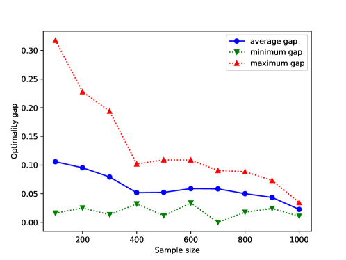
Figure 3: Optimality gap under different sample size (simulated dataset)

Finally, we apply the AGD algorithm to the pricing problem in the electricity industry under real conditions. We divided the dataset into two parts, the training set (n = 1895, 90%) and the test set (n = 211, 10%). We generate an approximate model based on the training set data and sample the historical features from the test set to before using them to solve the pricing problem. We assume that the pricing data in the test set is reasonable, so we can compare the decisions made by algorithm with the actual prices to judge the rationality of the algorithm results. The results in Figure 4 show that the difference between the most pricing decision given by the AGD algorithm and the actual pricing is within 5%.

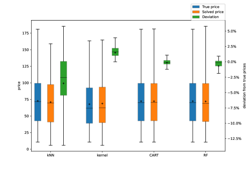
Figure 4: Comparison between historical price and optimization result (real dataset)

4.3 Value of Decision Dependent Property

In this section, we demonstrate the necessity of considering the decision-dependent characteristic of our model. Remind that the decision-dependent models are those in which the distribution of stochastic parameters, for example the demands, depend on the decision itself, rather than being determined solely by the features. Failure to account for this property can lead to significant errors in the solution obtained. We will compare two solution approaches: the decision-dependent scenario solved by AGD and the decision-independent scenario solved by reliable optimization tools. We show that accounting for the decision-dependent nature of the problem is crucial for obtaining accurate solutions.

We first describe the two scenarios mentioned above. In the decision-dependent scenario, we construct approximate model as (4) and use AGD algorithm to solve the model. In the decision-independent scenario, however, we construct the approximate model in the same way as the decision-dependent scenario. The only difference is that we delete the price variable $p$ from the weight function $w^{i}(\cdot)$. We use the minimization function in ”scipy” package in Python, since the removal of decision variable from the weight function significantly reduces the complexity of the approximate model. We also study the performance of pure SAA method, which ignores both decision-dependent effect and feature (see Section 7.4 for detail).

We conduct the comparison on both simulated and real-world datasets. In the simulated dataset experiments, we compare the objective function obtained from the two scenarios. In the real-world dataset, since we are unable to determine the true objective function due to the unknown demand distribution, we instead assume that the historical pricing decisions in the test set are reasonable. We then compare the optimization results obtained from decision-dependent, decision-independent and pure SAA scenarios to the historical prices in the test set. We set the deviation from the historical prices as a criterion of the performance of the algorithm.

The result on the simulated dataset shown in Table 1, where the gap reduction is the difference between decision-independent approach and decision-dependent approach. When the decision-dependent characteristic of the problem is taken into account, the AGD algorithm can converge to a local minimum in the vicinity of the true optimum. However, when the decision-dependent is not taken into consideration, the obtained solution is significantly biased away from the true optimum.

Table 1: Comparison between decision-dependent and decision-independent scenarios (real dataset).

Method	Decision-dependent scenarios
	kNN	kernel	CART	RF
Profit	674.37	698.2	689.94	584.07
Optimality gap	4.03%	0.64%	1.82%	16.88%
Gap reduction	96.93%	99.51%	98.49%	86.41%
Method	Decision-independent scenarios
	kNN	kernel	CART	RF	pure SAA
Profit	-220.88	-212.52	-139.59	-170.46	-283.62
Optimality gap	131.43%	130.24%	119.87%	124.26%	140.36%

The results of the real-world pricing problem can be seen in Figure 5. When the decision-dependent characteristic of the problem is considered, the obtained pricing decision is close to the true historical price, while the solution obtained under the decision-independent assumption was significantly biased away from the historical prices, which is consistent with the simulated dataset.

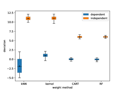
Figure 5: Deviation comparison between decision dependent and independent scenarios (real dataset)

In summary, we demonstrate the importance of accounting for the decision-dependent characteristic of our weight approximation model. In both simulated and practical dataset, failure to consider the decision-dependent characteristic can result in significant errors in the solution obtained. This proves the necessity of decision-dependent characteristic and hence illustrates the importance of AGD algorithm that can solve this kind of problem.

4.4 Value of Distribution-Free Property

In this section, we validate the necessity and practical significance of the distribution-free property in our model. The experiments are designed to compare the performance of the distribution-free (DF) method with the traditional PTO approach in two scenarios with different demand distributions.

We generate two sets of demand samples, one with the simple linear decision rule where the demands have a linear relationship to the features and price, and the other with the complex demand model we used to generate simulated dataset (see Section 9.1). For each demand setting, we compare the performance of two solution approaches: the first approach is to use the PTO paradigm. We first construct the demand model $D(p,z)$ by linear regression trained by the dataset before substituting the demand model and optimizing the best price. The second approach is to use the distribution-free approximation model described in Section 2.1, and then solve the problem using the AGD algorithm.

The results of our experiments are shown in Figure 7(b). We can observe that in the simple linear demand model scenario, the PTO method outperforms the distribution-free method because the true demand model satisfies the demand prediction assumptions exactly. We also notice that even in this case, the distribution-free method still performs well. In contrast, in the complex demand distribution scenario, our DF method clearly outperforms the PTO method. Moreover, we find that when the demand prediction assumption deviates from the true distribution, the PTO strategy sometimes generates lower profits and sometimes fails to converge. Therefore, when there is few information about the distribution of stochastic parameters, adopting the distribution-free method can better adapt to a broader range of real-world scenarios, and lead to better solutions than assuming a specific distribution rule for unknown parameters.

Figure 6: Comparison between distribution-free (DF) and PTO approach under two demand models (simulated dataset)

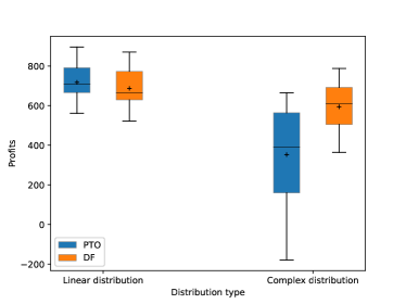
(a) Profits comparison between DF and PTO method under two demand models

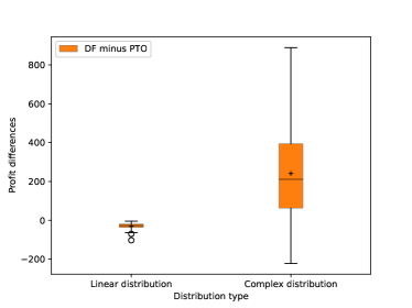
(b) Profit differences of DF and PTO method under two demand models

In summary, our experiments show that the distribution-free property is necessary and beneficial for our model. Though increases the complexity, it can help to overcome the challenge of estimating the unknown demand distribution, and is more robust to various distributional assumptions that may not hold in practice. The result also suggests that the AGD algorithm can handle the complexity brought by the distribution-free property.

5 Conclusion

In this work, we study a data-driven, decision-dependent newsvendor pricing problem. The demand distribution is unknown and depends on pricing decision. The demand has to be learned from the historical features and prices. We develop the approximation model to address the distribution-free characteristic of demand. But we find the decision-dependent characteristic brings significant complexity to the approximate model. Therefore, we develop the concept of approximate gradient and propose the AGD algorithm to efficiently and effectively solve the approximate model. We show that our the theoretical guarantee of our AGD algorithm under nonconvex, convex and strongly-convex conditions. Our simulation experiments demonstrate that our model can approximately converge to the local optimal point, even with a small sample size Moreover, the results on the real-world dataset indicates that the pricing decisions generated by the AGD algorithm are similar to those made in practice.

Our study finds that compare to the traditional newsvendor problem, the decision-dependent newsvendor pricing problem is important. Though the demand may not be solely determined by price, ignoring the impact of pricing decisions on demand can result in decisions that deviate significantly from the optimal profit. Furthermore, we highlight the advantages of data-driven methods, and provide insights into the priority of distribution-free methods. When the demand distribution is close to the predictive model, the PTO framework is preferred. But the predict model may fail when predicting the demand of new products or initial pricing. In these cases, the AGD algorithm-based data-driven approach can adapt to complex and unknown demand distributions and decision-dependent rule.

Our work is not limited to the study of inventory management problems. As shown in (4) and (8), neither the construction of approximate models nor the implementation of the AGD algorithm is dependent on the form of the profit function. Therefore, our work can be extended to most unconstrained decision-dependent models such as the strategic classification problem in ML. Moreover, the concept of approximate gradient is not limited by the specific approximation approach. In our work, we use the weight approximation method because it is effective in handling the decision-dependent property. The AGD algorithm can also adapt to other approximation approach such as SAA. It will achieve high accuracy if the corresponding approximate approach is reliable.

In our future work, we seek to apply the our data-driven method to multi-period inventory models. In multi-period models, the demand will depend not only on the current price but also on historical pricing decisions. The concept of price-adjustment cost will also be more important. To consider the optimal value of multi-period profit, we may combine data-driven approximation methods with dynamic programming methods. Transforming this type of multi-period inventory problem into a reinforcement learning problem and combining it with data-driven methods may also be a possible direction for future research. We are also interested in applying the concept of approximate gradient to constrained problems, since the gradient of constraint functions can also be approximated through the same approach, which can connect the approximate model to some convergence conclusions.

Wenxuan Liu acknowledges the support from the department of Industrial Engineering, Tsinghua University and is grateful for the support from the mentor. The authors are indebted to the department editor, senior editor, and referees for their valuable and constructive suggestions.

E-Companion for Solving Data-Driven Newsvendor Pricing Problems with Decision-Dependent Effect

6 Definition of Weight Functions

In this section, we present some definitions of the weight functions that can be used to construct the approximate model (4).

Definition 6.1 (Kernel regression weight)

We can use the kernel function that measures the distances in $(p,z)$ to construct the weight function:

$$w^{\mbox{KR},i}(p,z)=\frac{K_{h}\left((p,z)-(p^{i},z^{i})\right)}{\sum_{j=1}^{n}K_{h}((p,z)-(p^{j},z^{j}))}$$ (18)

where $K_{h}:\mathbb{R}^{dim(z)+1}\rightarrow\mathbb{R}$ is the kernel function with bandwidth $h$. Common kernel functions include the uniform kernel, triangular kernel and Gaussian kernel. If not noted, the kernel functions below refer to the Guassian kernel function:

$$K(z)=\frac{1}{\sqrt{2\pi}}\mbox{exp}^{-\|z\|_{2}^{2}/2}$$ (19)

Definition 6.2 (CART weight)

The CART weight functions are given by:

$$w^{\mbox{CART},i}(p,z)=\frac{\mathbb{I}\{R((p,z))=R((p^{i},z^{i}))\}}{|\{j:R((p^{j},z^{j}))=R((p,z))\}|}$$ (20)

where $R:Z\rightarrow\{1,...,r\}$ is the function that maps features to the $r$ leaves on the CART. In the CART, a leaf is a collection of sample points that are classified to the same group.

Definition 6.3 (Random forest weight)

The random forest weight functions are given by:

$$w^{\mbox{RF},i}(p,z)=\frac{1}{N_{E}}\sum^{N_{E}}_{e=1}w^{\mbox{CART},i,e}(p,z)$$ (21)

where $N_{E}$ is the number of estimators in the random forest, and $w^{\mbox{CART},i,e}(p,z)$ is the CART weight of the $e$th estimator in the random forest.

One of the advantage of random forest weight is that the variance will not get large as $N_{E}$ increases, while the estimation will be more accurate. The only cost is that it will consume more time to calculate the random forest weight if $N_{E}$ become larger.

7 Description of Solution Methods

In this section, we explain the solution methods adopted in the numerical experiment section.

7.1 Diminishing Step

The diminishing step adopt the step size $\eta^{r}$ such that $\eta^{r}>\eta^{r+1}$ and $\sum_{r=0}^{\infty}\eta^{r}=\infty$. A typical choice is $\eta^{r}=C/(r+1)$, where $C$ is a constant that can be adjusted to suit different problems.

7.2 Armijo Step

Let $f(\cdot)$ denote the objective function we want to minimize. The Armijo principle chooses the step size $\eta^{r}$ by the following steps (we denote the approximate gradient as $G^{N}$ and the ascent direction as $d^{r}$) in algorithm 2

Algorithm 2 Armijo step size

1:iteration solution $x^{r}$, $\alpha_{0}$, $\beta\in(0,1)$, $\sigma\in[0,1)$, tolerance $\epsilon$.

2:step size $\eta^{r}$;

3:$\eta^{r}=\alpha_{0}$;

4:$x^{r+1}=x^{r}+\eta^{r}d^{r}$.

5:while $\eta^{r}\geq\epsilon$ and $f(x^{r})-f(x^{r+1})<\sigma\eta^{r}(G^{N})^{T}d^{r}$ do

6:     $\eta^{r}=\eta^{r}*\beta$;

7:     $x^{r+1}=x^{r}+\eta^{r}d^{r}$.

8:end while

9:if $\eta^{r}<\epsilon$ then

10:     return Stop the iteration

11:else

12:     return $\eta^{r}$

13:end if

Note that the hyperparameter $\sigma$ can be $0$ in our problem. When $\sigma=0$, the armijo step size ensure that the objective function descent in an approximate context. We also show the special meaning when $\sigma=0$ in Proposition 3.2.

7.3 Decision-independent approach

The decision independent approach adopt a different model than the AGD algorithm:

$$\mbox{({Decision-independent Model})}\min_{p,q}\hat{f}(p,q;z)\overset{def}{=}\sum_{i=1}^{N}w^{i}(z)l_{a}(p,q,D^{i}),$$ (22)

The only difference between (22) and the original approximate model (4) is the variables in the weight function. In the decision-independent model, we remove the decision variable from the weight function as an ignorance of the decision-dependent effect. We then use some optimization tool to solve (22) since it is much easier to solve without the appearance of decision variables in the weight function. We can also use AGD algorithm to solve (22) but the solution sequence is not convergent since the estimation on the gradient become worse without the consideration on the decision-dependent effect.

7.4 Pure SAA

The Pure SAA approach is an approximate model that ignores features:

$$\mbox{({Pure SAA Model})}\min_{p,q}\hat{f}(p,q;z)\overset{def}{=}\frac{1}{n}\sum_{i=1}^{N}l_{a}(p,q,D^{i}),$$ (23)

The pure SAA model ignores both the decision-dependent effect and the feature. It can be treated as a decision-independent model without feature or an approximate model with kNN $k=N$ weight function.

7.5 Predict-then-optimize

The predict-then-optimize approach first predict the demand by applying linear regression on the training set. After performing the linear regression, we get the demand function $D(p,z)$. Then we can substitute the demand in the cost function $l(p,q,D)$ with $D(p,z)$ and optimize the model on $p,q$. Note that the prediction method is not limited to linear regression, all predict approaches that can lead to a demand function $D(p,z)$ can fit the PTO paradigm.

8 Proofs

Proof 8.1

Proof of Proposition 2.3 Proposition 2.3 is actually a corollary of theorem EC.9 in Bertsimas and Kallus (2019). To prove the proposition, we only need to validate the assumptions.

Since for every $p$, the marginal distribution of $D,Q\sim f_{D}(p,z)$ is independent of $p$ conditioned on $z$, the ignorability assumption satisfies. The cost gradient defined in (7) is well defined since the historical demand and supply cannot go to infinity. And it is also equicontinuous. The feasible region for $p,q$ is nonempty, closed and bounded we only restrict the up and down limit of the two decisions. Therefore, Proposition 2.3 follows by EC.9 in Bertsimas and Kallus (2019).

Proof 8.2

Proof of Proposition 2.4 Assume that for any $p,q,z$, the value range of $D$ remains to be the same set $\Omega$. We rewrite the objective expectation to the integrate form:

$$\partial_{p,q}\mathbb{E}_{D\sim f_{D}(p,z)}[l(p,q,D)]=\partial{p,q}\int_{D\in\Omega}l(p,q,D)f_{D}(p,q,D)dD$$

Suppose that the derivative of $l(p,q,D)f_{D}(p,q,D)$ can be bounded by an $L^{1}$ function $g$ for all $p,q,D,Q$, then the derivative and integration operator can be switched.

$$\partial_{p,q}\mathbb{E}_{D\sim f_{D}(p,z)}[l(p,q,D)]= \int_{D\in\Omega}\partial_{p,q}\left(l(p,q,D)f_{D}(p,q,D)\right)dD$$

$$= \int_{D\in\Omega}\left(\partial_{p,q}l(p,q,D)\right)f_{D}(p,q,D)dD$$

$$+\int_{D\in\Omega}\left(\partial_{p,q}f_{D}(p,q,D)\right)l(p,q,D)dD$$

$$= \mathbb{E}_{D\sim f_{D}(p,z)}[\partial_{p,q}l(p,q,D)]$$

$$+\int_{D\in\Omega}\left(\partial_{p,q}f_{D}(p,q,D)\right)l(p,q,D)dD$$

Generally, the second term of the last equation is not $0$. So the expectation of cost gradient do not equal to the gradient of objective expectation and thus the convergence of approximate gradient fails.

Before we begin to proof the convergence results, we first state some important results. The following lemmas show how Assumption 3.1 affects the distance between expectations of different distributions.

Lemma 8.3

Kantorovich-Rubinstein For all function $f$ that is $1-$Lipschitz

$$\|\mathbb{E}_{d\sim D(p)}\mathbb{E}[f(d)]-\mathbb{E}_{d\sim D(p^{\prime})}\mathbb{E}[f(d)]\|\leq W_{1}(D(p),D(p^{\prime}))$$

Lemma 8.4

Suppose Assumption 3.1 holds. Let $f:R^{n}\rightarrow R^{d}$ be an $L-$Lipschitz function, and let $X,X^{\prime}\in\mathbb{R}^{n}$ be random variables such that $W_{1}(X,X^{\prime})\leq C$. Then

$$\|\mathbb{E}[f(X)]-\mathbb{E}[f(X^{\prime})]\|_{2}\leq LC$$ (24)

Proof 8.5

Proof of Lemma 8.4

Since

$$\|\mathbb{E}[f(X)]-\mathbb{E}[f(X^{\prime})]\|_{2}^{2} =(\mathbb{E}[f(X)]-\mathbb{E}[f(X^{\prime})])^{T}(\mathbb{E}[f(X)]-\mathbb{E}[f(X^{\prime})])$$

$$=\|\mathbb{E}[f(X)]-\mathbb{E}[f(X^{\prime})]\|_{2}\frac{(\mathbb{E}[f(X)]-\mathbb{E}[f(X^{\prime})])^{T}}{\|\mathbb{E}[f(X)]-\mathbb{E}[f(X^{\prime})]\|_{2}}(\mathbb{E}[f(X)]-\mathbb{E}[f(X^{\prime})])$$

we define the unit vector $e:=\frac{(\mathbb{E}[f(X)]-\mathbb{E}[f(X^{\prime})])^{T}}{\|\mathbb{E}[f(X)]-\mathbb{E}[f(X^{\prime})]\|_{2}}$, we can get:

$$\|\mathbb{E}[f(X)]-\mathbb{E}[f(X^{\prime})]\|_{2}^{2}=\|\mathbb{E}[f(X)]-\mathbb{E}[f(X^{\prime})]\|_{2}(\mathbb{E}[e^{T}f(X)]-\mathbb{E}[f(X^{\prime})])$$

Since $f$ is a one-dimensional $L-$lipschitz function, we can apply Lemma 8.3 and Assumption 3.1 to obtain that for all $e$,

$$\|\mathbb{E}[f(X)]-\mathbb{E}[f(X^{\prime})]\|_{2}^{2}\leq\|\mathbb{E}[f(X)]-\mathbb{E}[f(X^{\prime})]\|_{2}LC$$

Thus completing the proof

Proof 8.6

Proof of Proposition 3.1

The proof is divided into two steps. In the first step, we prove that the objective function $\mathbb{E}_{D\sim f_{D}(x,D)}[l(x,D)]$ has Lipschitz gradient in $x$. Then we prove that under diminishing step, any converging subsequence converge to the stationary point.

We denote $f(x)=\mathbb{E}_{D\sim f_{D}(x,D)}[l(x,D)]$, then

$$\|\nabla_{x}f(x)-\nabla_{x}f(y)\|=\|\nabla_{x}\mathbb{E}_{D\sim f_{D}(x,D)}[l(x,D)]-\nabla_{x}\mathbb{E}_{D\sim f_{D}(y,D)}[l(y,D)]\|$$

According to Assumption 3.1, we can write the expectation to integrate form and change the integrate operator and derivative operator.

$$\|\nabla_{x}f(x)-\nabla_{x}f(y)\|= \|\int_{D\in\Omega}\nabla_{x}(l(x,D)f_{D}(x,D))dv-\int_{D\in\Omega}\nabla_{x}(l(y,D)f_{D}(y,D))dv\|$$

$$\leq \|\int_{D}l(x,D)(\nabla_{x}f_{D}(x,D))-l(y,D)(\nabla_{x}f_{D}(y,D))dv\|$$

$$+\|\int_{D}(\nabla_{x}l(x,D))f_{D}(x,D)-(\nabla_{x}l(y,D))f_{D}(y,D)dv\|$$

$$= I+II$$

The second inequality follows by the multiplication rule of derivative. We then analyze $I$ and $II$ respectively.

$$I\leq \|\int_{D}l(x,D)\nabla_{x}f_{D}(x,D)dv-\int_{D}l(x,D)\nabla_{x}f_{D}(y,D)dv\|$$

$$+\|\int_{D}l(x,D)\nabla_{x}f_{D}(y,D)dv-\int_{D}l(y,D)\nabla_{x}f_{D}(y,D)dv\|$$

$$\leq \int_{D}|l(x,D)|\|\nabla_{x}f_{D}(x,D)-\nabla_{x}f_{D}(y,D)\|dv$$

$$+\int_{D}|l(x,D)-l(y,D)|\|\nabla_{x}f_{D}(y,D)\|dv$$

$$\leq S_{\Omega}L_{4}L_{3}\|x-y\|+S_{\Omega}L_{5}L_{1}\|x-y\|$$

The first inequality holds from the triangular inequality. The second inequality holds by the Cauchy-Schwarz inequality. The third inequality holds by the Lipschitz continuous characteristic and intermediate value theorem, where $S_{\Omega}$ denotes of the set $\Omega$.

We can also bound the second term by the following steps:

$$II\leq \|\int_{D}\nabla_{x}l(x,D)f_{D}(x,D)dv-\int_{D}\nabla_{x}l(x,D)f_{D}(y,D)dv\|$$

$$+\|\int_{D}\nabla_{x}l(x,D)f_{D}(y,D)dv-\int_{D}\nabla_{x}l(y,D)f_{D}(y,D)dv\|$$

$$= \|\mathbb{E}_{D\sim f_{D}(x,D)}[\nabla_{x}l(x,D)]-\mathbb{E}_{D\sim f_{D}(y,D)}\nabla_{x}l(x,D)\|+\|\mathbb{E}_{D\sim f_{D}(y,D)}[\nabla_{x}l(x,D)-\nabla_{x}l(x,D)]\|$$

$$\leq \epsilon L_{2}\|x-y\|+L_{2}\|x-y\|$$

The first inequality holds by the triangular inequality. The first equality holds by the definition of expectation. The second inequality holds by Lemma 8.4 and the definition of Lipschitz gradient.

Thus, $\|\nabla_{x}f(x)-\nabla_{x}f(y)\|\leq[(\epsilon+1)L_{2}+S_{\Omega}(L_{1}L_{5}+L_{4}L_{3})]\|x-y\|$. Hence the objective function has Lipschitz gradient and $L=(\epsilon+1)L_{2}+S_{\Omega}(L_{1}L_{5}+L_{4}L_{3})$.

recall that the update rule is given by

$$x^{r+1}_{N}=x^{r}_{N}+\eta^{r}G^{N}(x;z)$$

From descent lemma, we have

$$f(x^{r+1}_{N})\leq f(x^{r}_{N})+\eta^{r}G^{N}(x^{r}_{N};z)^{T}\nabla f(x^{r}_{N})+\frac{L(\eta^{r})^{2}}{2}\|G^{N}(x^{r}_{N};z)\|^{2}$$

Taking $N\rightarrow\infty$ on both sides, since $f(x)$ is continuous and $\lim_{N\rightarrow\infty}G^{N}(x;z)=\mathbb{E}_{D\sim f_{D}(x,D)}[\nabla_{x}l(x,D)]$ from Proposition 2.3.

$$f(x^{r+1})-f(x^{r})\leq\eta^{r}\mathbb{E}_{D\sim f_{D}(x^{r},D)}[\nabla_{x}l(x^{r},D)]^{T}\nabla f(x^{r})+\frac{L(\eta^{r})^{2}}{2}\|\mathbb{E}_{D\sim f_{D}(x^{r},D)}[\nabla_{x}l(x^{r},D)]\|^{2}$$

where $x^{r}=\lim_{N\rightarrow\infty}x^{r}_{N}$.

Since

$$\mathbb{E}_{D\sim f_{D}(x^{r},D)}[\nabla_{x}l(x^{r},D)]^{T}f(x^{r})= \|\nabla_{x}\mathbb{E}_{D\sim f_{D}(x^{r},D)}[l(x^{r},D)]\|^{2}+\|\mathbb{E}_{D\sim f_{D}(x^{r},D)}[\nabla_{x}l(x^{r},D)]\|^{2}$$

$$-\|\int_{D}l(x^{r},D)\nabla_{x}f_{D}(x^{r},D)dv\|^{2}$$

$$\geq (\|\nabla_{x}\mathbb{E}_{D\sim f_{D}(x^{r},D)}[l(x^{r},D)]\|^{2}-L_{4}^{2}L_{5}^{2}S^{2}_{\Omega})+\|\mathbb{E}_{D\sim f_{D}(x^{r},D)}[\nabla_{x}l(x^{r},D)]\|^{2}$$

Note that since the range of $D$ is limited, we can scale the random parameters $D$ so that $S_{\Omega}$ is sufficiently small. Thus

$$\mathbb{E}_{D\sim f_{D}(x^{r},D)}[\nabla_{x}l(x^{r},D)]^{T}f(x^{r})\geq\|\mathbb{E}_{D\sim f_{D}(x^{r},D)}[\nabla_{x}l(x^{r},D)]\|^{2}$$

Therefore,

$$f(x^{r+1})-f(x^{r})\leq-\eta^{r}(1-\frac{L\eta^{r}}{2})\|\mathbb{E}_{D\sim f_{D}(x^{r},D)}[\nabla_{x}l(x^{r},D)]\|^{2}$$

Since $\eta^{r}$ is diminishing, for any $\xi\in(0,1)$, there exists $\bar{r}$ such that for any $r\geq\bar{r}$, we have

$$f(x^{r+1})-f(x^{r})\leq-\eta^{r}\xi\|\mathbb{E}_{D\sim f_{D}(x^{r},D)}[\nabla_{x}l(x^{r},D)]\|^{2}$$

Since $\lim_{r\in\mathcal{K}\rightarrow\infty}x^{r}=\bar{x}$ and $f(x)$ is continuous, we have $\lim_{r\rightarrow\infty}f(x^{r})=f(\bar{x})$. Taking summation on both sides from $r=\bar{r}$ to $\infty$, we can obtain that

$$\sum_{r=\bar{r}}^{\infty}\eta^{r}\xi\|\mathbb{E}_{D\sim f_{D}(x^{r},D)}[\nabla_{x}l(x^{r},D)]\|^{2}\leq f(x^{\bar{r}})-\lim_{r\rightarrow\infty}f(x^{r})$$

Since $\sum_{r=\bar{r}}^{\infty}\alpha^{r}=+\infty$, we have $\lim_{r\in\mathcal{K}\rightarrow\infty}\|\mathbb{E}_{D\sim f_{D}(x^{r},D)}[\nabla_{x}l(x^{r},D)]\|^{2}=0$, hence $\mathbb{E}_{D\sim f_{D}(\bar{x},D)}[\nabla_{x}l(\bar{x},D)]=0$ and the proof is completed.

Proof 8.7

Proof of Proposition 3.2 To simplify the denotation, we omit the limitation of $N\rightarrow\infty$. Therefore the descent direction is $d^{r}=-\mathbb{E}_{D\sim f_{D}(x^{r},D)}[\nabla_{x}l(x^{r},D)]$, where $x^{r}=\lim_{N\rightarrow\infty}x^{r}_{N}$. And we denote $f(x)=\mathbb{E}_{D\sim f_{D}(x^{r},D)}[l(x^{r},D)]$. According to the armijo principle:

$$f(x^{r})-f(x^{r+1})\geq-\eta^{r}\sigma\|\mathbb{E}_{D\sim f_{D}(x^{r},D)}[\nabla_{x}l(x^{r},D)]\|^{T}d^{r}$$

Since $\lim_{r(\in\mathcal{K})\rightarrow\infty}\sup_{r}\|\mathbb{E}_{D\sim f_{D}(x^{r},D)}[\nabla_{x}l(x^{r},D)]\|\geq 0$. The sequence $\mathbb{E}_{D\sim f_{D}(x^{r},D)}[l(x^{r},D)]$ decreases monotonically and have a lower bound. Thus

$$\lim_{r(\in\mathcal{K})\rightarrow\infty}f(x^{r})-f(x^{r+1})=0,$$

which is followed by

$$\lim_{r(\in\mathcal{K})\rightarrow\infty}\eta^{r}=0$$

Hence, by the definition of the armijo rule, we must have for some index $\bar{r}\geq 0$

$$f(x^{r})-f(x^{r}+\frac{\eta^{r}}{\beta}d^{r})<-\sigma\frac{\eta^{r}}{\beta}\|\mathbb{E}_{D\sim f_{D}(x^{r},D)}[\nabla_{x}l(x^{r},D)]\|^{T}d^{r},\forall r\in\mathcal{K},r\geq\bar{r}$$

We denote

$$p^{r}=\frac{d^{r}}{\|d^{r}\|},\quad\bar{\eta}^{r}=\frac{\eta^{r}\|d^{r}\|}{\beta}$$

Since $\|p^{r}\|=1$, there exists a subsequence $\{p^{r}\}_{\bar{\mathcal{K}}}$ of $\{p^{r}\}_{\mathcal{K}}$ such that $\{p^{r}\}_{\bar{\mathcal{K}}}\rightarrow\bar{p}$, where $\bar{p}$ is a unit vector. Then

$$\frac{f(x^{r})-f(x^{r+1})}{\bar{\eta}^{r}}<-\sigma(\mathbb{E}_{x^{r}\sim f_{x^{r}}(D,x^{r})}[\nabla_{x}l(D,x^{r})])^{T}p^{r}$$

Hence,

$$\frac{f(x^{r})-\mathbb{E}_{D\sim f_{D}(x^{r})}[l(x^{r+1},D)]+\mathbb{E}_{D\sim f_{D}(x^{r})}[l(x^{r+1},D)]-f(x^{r+1})}{\bar{\eta}^{r}}<-\sigma(\mathbb{E}_{x^{r}\sim f_{x^{r}}(D,x^{r})}[\nabla_{x}l(D,x^{r})])^{T}p^{r}$$ (25)

By Lemma 8.4, $f(x^{r})-f(x^{r+1})\geq-\epsilon L_{1}\|\bar{\eta}^{r}p^{r}\|$

By using the mean value theorem,

$$\frac{-\epsilon L_{1}\|\bar{\eta}^{r}p^{r}\|}{\bar{\eta}^{r}} +\mathbb{E}_{D\sim f_{D}(x^{r})}[\nabla l(x^{r}+\tilde{\alpha}^{r}p^{r})]^{T}p^{r}$$ (26)

$$<-\sigma(\mathbb{E}_{x^{r}\sim f_{x^{r}}(D,x^{r})}[\nabla_{x}l(D,x^{r})])^{T}p^{r}$$

Let $r(\in\bar{\mathcal{K}})\rightarrow\infty$,

$$-\epsilon L_{1}-(\mathbb{E}_{D\sim f_{D}(\bar{x},D)}[\nabla_{x}l(\bar{x},D)])^{T}\bar{p}<-\sigma\mathbb{E}_{D\sim f_{D}(\bar{x},D)}[\nabla_{x}l(\bar{x},D)]^{T}\bar{p}$$

Substituting $d^{r}=-\mathbb{E}_{D\sim f_{D}(x^{r},D)}[\nabla_{x}l(x^{r},D)]$, we have

$$-\epsilon L_{1}<-(1-\sigma)\|\mathbb{E}_{D\sim f_{D}(\bar{x},D)}[\nabla_{x}l(\bar{x},D)]\|$$

which completes the proof.

Proof 8.8

Proof of Theorem 3.3 We proof the theorem by contradiction. Suppose $x^{*}$ maximize $\max_{x}f(x)=\mathbb{E}_{D\sim f_{D}(x,D)}[l(x,D)]$, and $\|\mathbb{E}_{D\sim f_{D}(x^{*},D)}[\nabla_{x}l(x^{*},D)]\|>L_{1}\epsilon$. Then for any $x_{1}\in X$,

$$f(x_{1})-f(x^{*})= \left(\mathbb{E}_{D\sim f_{D}(x_{1},D)}[l(x_{1},D)]-\mathbb{E}_{D\sim f_{D}(x,D)}[l(x,D)]\right)$$

$$= \left(\mathbb{E}_{D\sim f_{D}(x_{1},D)}[l(x_{1},D)]-\mathbb{E}_{D\sim f_{D}(x^{*})}[l(x_{1},D)]\right)$$

$$+\left(\mathbb{E}_{D\sim f_{D}(x^{*})}[l(x_{1},D)]-\mathbb{E}_{D\sim f_{D}(x,D)}[l(x,D)]\right)$$

From Lemma 8.4, we have

$$|\mathbb{E}_{D\sim f_{D}(x_{1},D)}[l(x_{1},D)]-\mathbb{E}_{D\sim f_{D}(x^{*})}[l(x_{1},D)]|\leq L_{1}\epsilon\|x_{1}-x^{*}\|$$

For the second term, we expand $l(x_{1},D)$ at $x^{*}$ and obtain

$$\mathbb{E}_{D\sim f_{D}(x^{*})}[l(x_{1},D)]-\mathbb{E}_{D\sim f_{D}(x,D)}[l(x,D)]=\mathbb{E}_{D\sim f_{D}(x^{*})}[\nabla_{x}l(x^{*},D)]^{T}(x_{1}-x^{*})+o(\|x_{1}-x^{*}\|)$$

where $o(\|x_{1}-x^{*}\|)$ denotes the first-order infinitesimals to $\|x_{1}-x^{*}\|$. By substituting the two terms above and divide both sides by $\|x_{1}-x^{*}\|$, we obtain

$$\frac{f(x_{1})-f(x^{*})}{\|x_{1}-x^{*}\|}\geq-L_{1}\epsilon+\mathbb{E}_{D\sim f_{D}(x^{*})}[\nabla_{x}l(x^{*},D)]^{T}\frac{(x_{1}-x^{*})}{\|x_{1}-x^{*}\|}+\frac{o(\|x_{1}-x^{*}\|)}{\|x_{1}-x^{*}\|}$$

We let $x_{1}-x$ take the same direction of $\mathbb{E}_{D\sim f_{D}(x^{*},D)}[\nabla_{x}l(x^{*},D)]$, hence the second term on the right side becomes $\|\mathbb{E}_{D\sim f_{D}(x^{*},D)}[\nabla_{x}l(x^{*},D)]\|$. Therefore, for any $\xi>0$, there exists $x_{1}$ that is sufficiently close to $x^{*}$ such that

$$\frac{f(x_{1})-f(x^{*})}{\|x_{1}-x^{*}\|}\geq-L_{1}\epsilon+\|\mathbb{E}_{D\sim f_{D}(x^{*},D)}[\nabla_{x}l(x^{*},D)]\|-\xi$$

Since $\|\mathbb{E}_{D\sim f_{D}(x^{*},D)}[\nabla_{x}l(x^{*},D)]\|>L_{1}\epsilon$ and $\xi$ can be sufficiently small, we have $f(x_{1})-f(x^{*})>0$, which contradicts with the condition that $f(x^{*})$ is the optimal solution.

Proof 8.9

Proof of Theorem 3.5 We analyze the error of $x^{k+1}_{N}$:

$$\|x^{k+1}_{N}-x^{*}\|^{2}= \|x^{k}_{N}-\eta^{k}G^{N}(x^{k}_{N},D)-x^{*}\|^{2}$$

$$= \|x^{k}_{N}-x^{*}\|^{2}-2\eta^{k}G^{N}(x^{k}_{N},D)^{T}(x^{k}_{N}-x^{*})+(\eta^{k})^{2}\|G^{N}(x^{k}_{N},D)\|^{2}$$

let $N\rightarrow+\infty$ for both sides, denote $\lim_{N\rightarrow\infty}x^{k}_{N}$ as $x^{k}$ for simplicity. Since $\lim_{N\rightarrow\infty}G^{N}(x^{k}_{N},D)=\mathbb{E}_{D\sim f_{D}(x^{k},D)}[\nabla_{x}l(x^{k},D)]$ for any $x$, we have

$$\|x^{k+1}-x^{*}\|^{2}=\|x^{k}-x^{*}\|^{2}-2\eta^{k}\mathbb{E}_{D\sim f_{D}(x^{k},D)}[\nabla_{x}l(x^{k},D)]^{T}(x^{k}-x^{*})+(\eta^{k})^{2}\|\mathbb{E}_{D\sim f_{D}(x^{k},D)}[\nabla_{x}l(x^{k},D)]\|^{2}$$

We bound the second term by convexity of the cost function

$$\mathbb{E}_{D\sim f_{D}(x^{k},D)}[\nabla_{x}l(x^{k},D)]^{T}(x^{k}-x^{*})= \mathbb{E}_{D\sim f_{D}(x^{k})}[\nabla l(x^{k},D)^{T}(x^{k}-x^{*})]$$

$$\geq \mathbb{E}_{D\sim f_{D}(x^{k})}[l(x^{k},D)-l(x^{*},D)]$$

For the third term, we bound by Assumption 3.3.

$$\|\mathbb{E}_{D\sim f_{D}(x^{k},D)}[\nabla_{x}l(x^{k},D)]\|^{2}\leq L^{c}_{3}$$

Thus

$$2\eta^{k}\mathbb{E}_{D\sim f_{D}(x^{k})}[l(x^{k},D)-l(x^{*},D)]\leq-\|x^{k+1}-x^{*}\|^{2}+\|x^{k}-x^{*}\|^{2}+(\eta^{k})^{2}(L^{c}_{3})^{2}$$

We further investigate the right side. Since

$$\mathbb{E}_{D\sim f_{D}(x^{k})}[l(x^{k},D)-l(x^{*},D)]= -\mathbb{E}_{D\sim f_{D}(x^{k})}[l(x^{*},D)]+\mathbb{E}_{D\sim f_{D}(x^{*},D)}[l(x^{*},D)]$$

$$-\mathbb{E}_{D\sim f_{D}(x^{*},D)}[l(x^{*},D)]+\mathbb{E}_{D\sim f_{D}(x^{k})}[l(x^{k},D)]$$

$$\geq -|\mathbb{E}_{D\sim f_{D}(x^{k})}[l(x^{*},D)]-\mathbb{E}_{D\sim f_{D}(x^{*},D)}[l(x^{*},D)]|$$

$$-\mathbb{E}_{D\sim f_{D}(x^{*},D)}[l(x^{*},D)]+\mathbb{E}_{D\sim f_{D}(x^{k},D)}[l(x^{k},D)]$$

$$\geq -\epsilon L^{c}_{2}\|x^{*}-x^{k}\|-\mathbb{E}_{D\sim f_{D}(x^{*},D)}[l(x^{*},D)]+\mathbb{E}_{D\sim f_{D}(x^{k},D)}[l(x^{k},D)]$$

Thus

$$2\eta^{k}(\mathbb{E}_{D\sim f_{D}(x^{k},D)}[l(x^{k},D)]-\mathbb{E}_{D\sim f_{D}(x^{*},D)}[l(x^{*},D)])\leq 2\eta^{k}\epsilon L^{c}_{2}\|x^{*}-x^{k}\|-\|x^{k+1}-x^{*}\|^{2}$$

$$+\|x^{k}-x^{*}\|^{2}+(\eta^{k}L^{c}_{3})^{2}$$

Take summation from $r=0$ to $k$ and take the minimum of the left side, we obtain

$$(2\sum_{r=0}^{k}\eta^{r})\min_{0\leq r\leq k}\{\mathbb{E}_{D\sim f_{D}(x^{r},D)}[l(x^{r},D)]-\mathbb{E}_{D\sim f_{D}(x^{*},D)}[l(x^{*},D)]\}\leq 2\epsilon L^{c}_{2}\sum_{r=0}^{k}\eta^{r}\|x^{*}-x^{k}\|$$

$$+\|x^{0}-x^{k}\|^{2}+(L^{c}_{3})^{2}\sum_{r=0}^{k}(\eta^{r})^{2}$$

Hence complete the proof.

Proof 8.10

Proof of Corollary 3.6 We need to determine $L^{c}_{2}$, $L^{c}_{3}$ in Theorem 3.5. Since $\nabla_{p}l(p,q,D)=-(D\wedge q)$, we have $L^{c}_{3}\leq(D\wedge q)$. We can rewrite the cost function to $l(p,q,D)=-(p-c)q+(p-s)(q-D)^{+}$, therefore, $L^{c}_{2}=1$. Then we substitute $L^{c}_{2}$ and $L^{c}_{3}$ into Theorem 3.5 complete the proof.

Proof 8.11

Proof of Theorem 3.7 We investigate the distance between $x^{k}_{N}$ and a stable point $x_{PS}$.

$$\|x^{k+1}_{N}-x_{PS}\|^{2}= \|x^{k}_{N}-\eta G^{N}(x^{k}_{N};z)-x_{PS}\|^{2}$$

$$= \|x^{k}_{N}-x_{PS}\|^{2}-2\eta G^{N}(x^{k}_{N})^{T}(x_{N}^{k}-x_{PS})+(\eta^{2})\|G^{N}(x^{k}_{N})\|^{2}$$

We begin by upper bounding the second term. From Proposition 2.3, we know that for any $\xi>0$, there exists a sample size $N_{0}$ such that $\sup_{x}\|G^{N}(x)-\mathbb{E}_{D\sim f_{D}(x,D)}[\nabla_{x}l(x,D)]\|\leq\xi$ for all $N>N_{0}$. Thus we have

$$G^{N}(x^{k}_{N})^{T}(x^{k}_{N}-x_{PS})\geq \mathbb{E}_{D\sim f_{D}(x^{k}_{N},D)}[\nabla_{x}l(x^{k}_{N},D)]^{T}(x^{k}_{N}-x_{PS})-\xi\|x^{k}_{N}-x_{PS}\|$$

We can further bound the first term using the same approach as the proof of proposition 2.3 in Mendler-Dünner et al. (2020b)’s work. They give that

$$\mathbb{E}_{D\sim f_{D}(x^{k}_{N},D)}[\nabla_{x}l(x^{k}_{N},D)]^{T}(x^{k}_{N}-x_{PS})\geq B\|x^{k}_{N}-x_{PS}\|^{2}$$

We then bound the third term:

$$\|G^{N}(x^{k}_{N})\|^{2}\leq\xi^{2}+\|\mathbb{E}_{D\sim f_{D}(x^{k}_{N},D)}[\nabla_{x}l(x^{k}_{N},D)]\|^{2}$$

We can also adopt the same approach in the proof of proposition 2.3 in Mendler-Dünner et al. (2020b). They give that under Assumption 3.3 and 3.1,

$$\|\mathbb{E}_{D\sim f_{D}(x^{k}_{N},D)}[\nabla_{x}l(x^{k}_{N},D)]\|^{2}\leq 2B^{2}\|x^{k}_{N}-x_{PS}\|^{2}$$

Therefore, we obtain

$$\|x^{k+1}_{N}-x_{PS}\|^{2}\leq(1-2\eta A+2\eta^{2}B^{2})\|x^{k}_{N}-x_{PS}\|^{2}+2\eta\xi\|x^{k}_{N}-x_{PS}\|+\xi^{2}\eta^{2}$$ (27)

In case 1, to give a reasonable distance bound, we need to choose $\eta$ such that the right-hand side is a perfect quadratic polynomial. Thus we choose $\eta$ such that

$$4B^{2}\eta^{2}-2A\eta+1=0$$

Note that from the Viete’s theorem, the two solutions are both positive since we assume $A>0$. Thus we only need to ensure that the equation have real solution, that is

$$4A^{2}\geq 16B^{2},\quad A\geq 2B$$

And we take the square root two both sides of equation (27)

$$\|x^{k+1}_{N}-x_{PS}\|\leq\sqrt{1-2\eta A+2\eta^{2}B^{2}}\|x^{k}_{N}-x_{PS}\|+\xi\eta$$

We denote $C=\sqrt{1-2\eta A+2\eta^{2}B}$ and divide both sides by $C^{k+1}$

$$\frac{\|x^{k+1}_{N}-x_{PS}\|}{C^{k+1}}\leq\frac{\|x^{k}_{N}-x_{PS}\|}{C^{k}}+\frac{\xi\eta}{C^{k+1}}$$

Take the summation on both sides from $0$ to $k+1$ and we obtain

$$\|x^{k+1}_{N}-x_{PS}\|\leq C^{k+1}\|x^{1}_{N}-x^{*}\|+\xi\eta\frac{1-C^{k+1}}{1-C}$$

Note that $\eta A-\eta^{2}B^{2}=\frac{2\eta A+1}{4}>0$, thus $C<1$ and the distance is decreasing.

Now we focus on case 2. Since the quadratic term on the right-hand side of (27) is less than zero, we obtain

$$\|x^{k+1}_{N}-x_{PS}\|^{2}\leq 2\eta\xi\|x^{k}_{N}-x_{PS}\|+\xi^{2}\eta^{2}$$ (28)

Thus

$$\|x^{k+1}_{N}-x_{PS}\|^{2}-\|x^{k}_{N}-x_{PS}\|^{2}\leq-\|x^{k}_{N}-x_{PS}\|^{2}+2\eta\xi\|x^{k}_{N}-x_{PS}\|+\xi^{2}\eta^{2}$$

If $\|x^{k}_{N}-x_{PS}\|\geq(1+\sqrt{2})\xi\eta$, we can derive that $\|x^{k+1}_{N}-x_{PS}\|^{2}-\|x^{k}_{N}-x_{PS}\|^{2}\leq 0$, which indicates that although the distance may exceed the bound $(1+\sqrt{2})\xi\eta$ some time, it will decrease immediately until it reach the bound, hence complete the proof.

Proof 8.12

Proof of Corollary 3.9 The corollary is proved by imposing the triangular inequality to Lemma 3.8 and Theorem 3.7.

Proof 8.13

Proof of Corollary 3.10 We observe that $l_{a}$ is $\gamma$-strongly convex on $p$. We first give the value of $L^{c}_{1}$ and $L_{D}$ in the price-adjustment case. Since $l_{a}(p,q,D)=(p-\tilde{p})^{2}-(p-c)q+(p-s)(q-D)^{+}$, we have $L_{D}=1$. And $\nabla_{p}l_{a}(p,q,D)=-(q\wedge D)+2\gamma(p-\tilde{p})$. we have $L_{1}^{c}\leq 2\gamma|p_{m}-\tilde{p}|$. Then the proof is complete by using the conclusion in Corollary 3.9.

9 Experiment Supplements

9.1 Description of data

Table 2: Description of real electricity pricing data

Variable	Type	Description	Statistics
Date	datetime	the date of the recording	min 1Jan15, max 6Oct20
Demand	float	a total daily electricity demand in MWh	min 85.1k, median 120k, max 171k
RRP	float	a recommended retail price in AUD$/MWh	min 0, median 66.7, max 300
min temperature	float	minimum temperature during the day in Celsius	min 0.6, median 11.3, max 28
max temperature	float	maximum temperature during the day in Celsius	min 9, median 19.1, max 43.5
solar exposure	float	total daily sunlight energy in MJ/m2̂	min 0.7, median 12.7, max 33.3
rainfall	float	daily rainfall in mm	min 0, median 0, max 54.6
school day	boolean	if students were at school on that day	True 69%, False 31%
holiday	boolean	if the day was a state or national holiday	True 4%, False 96%

Real data The real dataset comes from a real-world power plant pricing scenario (https://www.kaggle.com/datasets/aramacus/electricity-demand-in-victoria-australia). This dataset describes the electricity demand and price situation in Victoria, Australia from 2015 to 2020. The distribution of demand can be seen in Figure 7. The descriptive information of the real data is shown in Table 2. The factors that influence daily demand are price, temperature, solar exposure, school day and holiday. Note that we perform an artificial transformation on the temperature. We define heating degree day (HDD) as $HDD=(15-T_{max})^{+}$, and cooling heating degree day (CDD) as $CDD=(T_{min}-18)^{+}$, where $T_{max}$ and $T_{min}$ are the highest and lowest centigrade temperatures in one day. This transformation can better reflect the relationship between temperature and electricity demand. The demand is sensitive to price, but it also depend on other features such as temperature and holiday. In our work, we consider the temperature, solar, rainfall, school_day and holiday factors. Note that the scales of features are different, so we standardize the feature to $[0,1]$ when processing the data. We use Euclidean metric to measure the distance between samples.

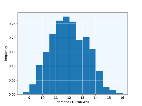
Figure 7: Demand distribution for real data

Simulation data In terms of simulation data, we generate the demand by the following model.

$$D=\max\{0,60-p+12a^{T}(X+0.25\phi)+5b^{T}X\theta\}$$ (29)

where $\phi\sim N(0,I_{4})$ is a $4$-dimensional vector, $\theta\sim N(0,1)$ is also a Guassian parameter. Both $\theta$ and $\phi$ are the stochastic factors that cause demand fluctuation. The constant vector $a=(0,8,1,1,1)^{T}$ and $b=(-1,1,0,0)^{T}$. Note that we refer the demand model to Lin et al. (2022). The demand distribution under $p=20$ is shown in Figure 8. We observe that the distribution is skew and long tail, thus hard to predict by simple models such as linear regression.

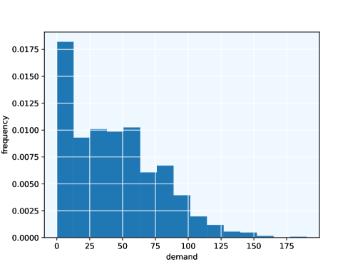
Figure 8: Demand distribution for simulated data

The second demand model is simply a linear regression model to suit the PTO assumption, where $D=60-p+(1,1,1,1)^{T}z+\phi$ and $\phi\sim N(0,1)$. Thus the demand follows a normal distribution under any price and feature.

9.2 Step size comparison

The step size of AGD algorithm adopted in the numerical experiment part is the Armijo step size with $\sigma=0$. In Section 3.2, we have analyzed the difference between the diminishing step size and Armijo step size. In this section, we will evaluate the difference by experiment.

We first compare two kinds of step size in the simulated dataset. We set the step size constant $C=0.05$ in diminishing step size approach. The realized profit and optimality gap are shown in Table 3. We can find that the diminishing step size performs worse than Armijo step size in this case. We believe the reason is that the assumptions for the convergence under diminishing step size are usually too strong. The value range $\Omega$ in Assumption 3.2 $L_{4}$ and $L_{5}$ constant in Assumption 3.2 maybe large in practice, causing a bad convergence performance. Moreover, we find that although any convergent subsequence converge to the local maximum according to Proposition 3.1, the diminishing step size cannot stop at the local maximum automatically, which indicates that the diminishing step size may not lead to any convergence subsequence. Therefore, the diminishing step size need a careful selection on the step size constant $C$ and stop criteria.

Table 3: Realized profit of Armijo step size and Diminishing step size

Method	kNN	kernel	CART	RF
Armijo	674.37	698.20	689.94	584.07
Diminishing	524.05	512.858	560.0039	388.8681

We also evaluate the effect of hyperparameter $\sigma$ on AGD algorithm. Table 4 reports the optimality gap and iteration number for different constant $\sigma$ under kernel regression . Figure 9 plots the supplementary result in terms of $\sigma$ and optimality gap. We observe the performance is stable when $\alpha_{0}\in(0.01,0.1)$, and when $\sigma\leq 0.2$. The increment of both $\alpha_{0}$ and $\sigma$ can reduce the iteration numbers, thus accelerate the solution. But when $\alpha_{0}$ is larger than $0.5$, the optimality gap may become larger. Larger $\sigma$ can block the update of solution and may cause the algorithm to stop before reaching the convergence.

Table 4: Performance comparison among different initial step sizes and $\sigma$ of Armijo step size

($\alpha_{0}$, $\sigma$)	profit	optimality gap	iterations	($\alpha_{0}$, $\sigma$)	profit	optimality gap	iterations
(0.01, 0)	695.89	0.97%	90	(0.5, 0)	672.02	4.37%	2
(0.01, 0.1)	688.28	2.05%	74	(0.5, 0.1)	691.25	1.63%	2
(0.01, 0.2)	659.48	6.15%	62	(0.5, 0.2)	667.36	5.03%	2
(0.01, 0.5)	475.37	32.35%	28	(0.5, 0.5)	562.69	19.92%	1
(0.01, 0.9)	300.00	57.31%	0	(0.5, 0.9)	300.00	57.31%	0
(0.05, 0)	698.20	0.64%	18	(1, 0)	653.18	7.05%	1
(0.05, 0.1)	688.84	1.97%	15	(1, 0.1)	653.18	7.05%	1
(0.05, 0.2)	662.67	5.70%	13	(1, 0.2)	653.18	7.05%	1
(0.05, 0.5)	478.73	31.87%	6	(1, 0.5)	569.02	19.02%	1
(0.05, 0.9)	300.00	57.31%	0	(1, 0.9)	300.00	57.31%	0
(0.1, 0)	696.72	0.85%	9
(0.1, 0.1)	689.42	1.89%	8
(0.1, 0.2)	659.40	6.16%	7
(0.1, 0.5)	491.16	30.10%	3
(0.1, 0.9)	300.00	57.31%	0

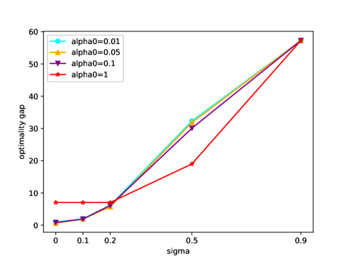
Figure 9: Performance comparison among different initial step sizes and $\sigma$ of Armijo step size

References

- Agrawal and Seshadri (2000) Agrawal, Vipul, Sridhar Seshadri. 2000. Impact of uncertainty and risk aversion on price and order quantity in the newsvendor problem. Manufacturing & Service Operations Management, 2 (4), 410-423.
- Ban and Rudin (2018) Ban, Gah-Yi, Cynthia Rudin. 2018. The big data newsvendor: Practical insights from machine learning. Operations Research, 67 (1), 90-108.