Sound velocity peak and conformality in isospin QCD

Abstract

We study zero temperature equations of state (EOS) in isospin QCD within a quark-meson model which is renormalizable and hence eliminates high density artifacts in models with the ultraviolet cutoff (e.g., NJL models). The model exhibits a crossover transition of pion condensations from the Bose-Einstein-Condensation regime at low density to the Bardeen-Cooper-Schrieffer regime at high density. The EOS stiffens quickly and approaches the quark matter regime at density significantly less than the density for pions to spatially overlap. The squared sound velocity $c_{s}^{2}$ develops a peak in the crossover region, and then gradually relaxes to the conformal value $1/3$ from above, in contrast to the perturbative QCD results which predicts the approach from below. In the context of QCD computations, this opposite trend is in part due to the lack of gluon exchanges in our model, and also due to the non-perturbative power corrections arising from the condensates. We argue that with large power corrections the trace anomaly can be negative. Our EOS reproduces the qualitative trend of the lattice results from the BEC to the BCS regime, implying that the quark-meson model captures relevant effective degrees of freedom. The BCS gap in our model is $\Delta\simeq 300$ MeV in the quark matter domain, and naive application of the BCS relation for the critical temperature $T_{c}\simeq 0.57\Delta$ yields the estimate $T_{c}\simeq 170$ MeV, in good agreement with the lattice data.

I Introduction

The quantum chromodynamics (QCD) with a large isospin chemical potential ($\mu_{I}$) can be studied in lattice Monte-Carlo simulations and hence has been a useful laboratory to test theoretical conceptions in dense matter [1, 2, 3]. In this theory, the positive isospin chemical potential favors the population of up-quarks and of down-antiquarks. A matter with finite isospin density starts with a Bose-Einstein-Condensation (BEC) phase of charged pions as composite particles. The dilute regime is well-described by chiral effective theories (ChEFT) for pions [4, 5, 6, 7, 8]. As density increases the quark substructure of pions should become important and the system transforms into a Bardeen-Cooper-Schrieffer (BCS) phase with a substantial quark Fermi sea. This BEC-BCS transition is crossover (for BEC-BCS crossover, see, e.g., Ref. [9, 10, 11]), as confirmed by model studies and lattice Monte-Carlo simulations. We study this crossover in the context of quark-hadron continuity [12, 13, 14] or duality [15, 16], which may be also realized in QCD at finite baryon chemical potential ($\mu_{B}$).

One of fundamental topics in dense QCD is the equation of state (EOS) (Ref. [17] for a short review from the QCD perspective), which is a crucial piece to understand the structure of neutron stars (NSs). Recent analyses of NSs, with similar radii ($\simeq 12.4$ km) for $2.1$ and $1.4$ solar mass NSs [18, 19, 20], and the nuclear physics constraints at nuclear saturation density $n_{0}$ ($\simeq 0.16\,{\rm fm}^{-3}$), suggest that the EOS stiffens rapidly (i.e., the pressure $P$ grows rapidly as a function of energy density $\varepsilon$) from low baryon density to high density, of $n_{B}=4$-$7n_{0}$, which is expected to be realized in the core of massive NSs. This stiffening accompanies the peak of sound velocity, $c_{s}=(\partial P/\partial\varepsilon)^{1/2}$; the $c_{s}^{2}$ is $\ll 1$ in the nuclear domain, goes beyond the so-called conformal value $1/3$, and relaxes to $1/3$ in the relativistic limit where the quark kinetic energy dominates over the interaction. While NS observations suggest such non-monotonic behaviors of $c_{s}$, it is necessary to understand the mechanisms from the microscopic physics. The sound velocity peak was first indicated in phenomenological interpolation of hadronic and quark matter EOS [21, 22, 23, 24], discussed in more general ground based on nuclear physics and NS observations by Ref. [25], and further elucidated in Refs. [26, 27, 28] utilizing the quark degrees of freedom. Recently more detailed descriptions have been attempted, see Refs. [29, 30, 31, 32, 33, 34, 35, 36, 37, 38], but it is difficult to directly test the scenarios. We use the isospin QCD for which lattice simulations are available, and delineate the behavior of $c_{s}^{2}$.

Another interesting question is how the $c_{s}^{2}$ approaches the conformal limit, $1/3$. Perturbative QCD (pQCD) [39, 40, 41, 42, 43, 44], which is supposed to be valid at $n_{B}\gtrsim 40n_{0}$, predicts that the $c_{s}^{2}$ approaches $1/3$ from below. The domain between $n_{B}\simeq 10n_{0}$ and $\simeq 40n_{0}$ has not been explored intensively. For this regime it is natural to regard quarks as relevant degrees of freedom but whose properties may be substantially renormalized by strong interaction effects [45, 46, 47]; if such interaction effects are properly absorbed into effective parameters of quasi-quarks, it is possible that the residual interactions may be treated in the same spirit as in constituent quark models for hadron physics. If this residual corrections are indeed smaller than the relativistic kinetic energy of quasi-particles, the system should show the conformal behavior even before achieving weakly correlated quark matter. How the matter reaches the conformal regime is intensively discussed in recent works [42, 48, 49, 50, 51, 52, 53].

We address the non-monotonic behavior of $c_{s}^{2}$ in isospin QCD within a renormalizable quark-meson model. The properties of the model in isospin QCD have been analyzed in detail by Refs. [54, 55, 56]. We follow their renormalization procedures. The advantage of using renormalizable effective models over models with a UV cutoff (e.g., the NJL models) is that one can temper the high density artifacts. In particular, the BCS type states have a distorted quark occupation probability whose high momentum tail reaches very high momenta, exceeding the UV cutoff. This is in contrast to the ideal gas case with the occupation probability $\theta(p-p_{f})$ which discontinuously drops to zero at the Fermi momentum $p_{f}$ before reaching the UV cutoff. In fact, NJL studies with BCS states exhibit growing $c_{s}^{2}$ toward the high density limit [57, 58]. In the quark-meson model such growing behaviors disappear; the $c_{s}^{2}$ relaxes to the conformal value $1/3$, as it should.

While our model predicts $c_{s}^{2}\rightarrow 1/3$, the conformal limit is reached from above, not from below as predicted in pQCD. The latter is due to the density dependence induced through the running $\alpha_{s}$. In the weak coupling limit and at high density, the only relevant scale is $\mu_{I}$ and the $c_{s}^{2}=1/3$ follows from $\partial(P/\mu_{I}^{4})/\partial\mu_{I}=0$. The first important corrections to the conformal limit come from the $\Lambda_{\rm QCD}\simeq$ 200-300 MeV in the running coupling constant. If we take into account $\Lambda_{\rm QCD}$ only in this way, the $c_{s}^{2}$ is reduced from $1/3$. Meanwhile, at the energy scale around $\sim 1\,{\rm GeV}$, it has been long known that power corrections of $\Lambda_{\rm QCD}$, which can not be expressed as perturbative series in $\alpha_{s}$, play important roles to capture the qualitative features in QCD [59, 60, 61]. Parametrizing pressure with power corrections as ($\chi_{I}$: isospin susceptibility)

$$P(\mu_{I})=a_{0}\mu_{I}^{4}+a_{2}\mu_{I}^{2}\,,$$ (1)

where $a_{2}\sim\Lambda_{\rm QCD}^{2}$, the squared sound velocity can be expressed as

$$c_{s}^{2}=\frac{\,n_{I}\,}{\,\mu_{I}\chi_{I}\,}=\frac{\,2a_{0}\mu_{I}^{2}+a_{2}\,}{\,6a_{0}\mu_{I}^{2}+a_{2}\,}\,.$$ (2)

For a positive $a_{2}$, the $c_{s}^{2}$ is larger than 1/3, and close to 1 if the $a_{2}$ term dominates. In our quark-meson model the $a_{2}$ is related to the pion condensates. We quantify the relation within our quark-meson model.

We briefly address the trace anomaly in dense matter which measures the breaking of the scale invariance [48, 49, 50]. We argue that changes from the non-perturbative to perturbative vacua add positive contributions to the trace anomaly, while the power corrections with $a_{2}>0$ favors the negative value. For large power corrections the trace anomaly can be negative. In this respect the sign of the trace anomaly is very useful to characterize the non-perturbative effects in dense quark matter.

For quantitative aspects, we confront our model calculations with the lattice results from two groups [62, 63]. Ref. [62] have more focus on the BEC regime while Ref. [63] covers more global nature up to the pQCD regime. Both groups agree in the BEC regime, and our model results are consistent with the lattice results. At high density, our model captures the overall trend of Ref. [63], especially the sound velocity peak and negative trace anomaly.

Since we are not sure about the convergence of loop expansion, as supplement studies we perform several parametric studies of EOS to examine several qualitative effects which we believe to be important. They are used to delineate the results of the quark-meson model in Sec.IV.

In this paper we use nuclear saturation density in QCD, $n_{0}=0.16\,{\rm fm}^{-3}$, as our unit for isospin density. While there is no need to address nuclear saturation in isospin QCD, our goal is to discuss physics as a step to understand NS EOS and $n_{0}$ is useful in this phenomenological context.

This paper is organized as follows. In Sec.II we discuss our set up for a quark meson model. The renormalization procedures are summarized. In Sec.III we present the renormalized thermodynamic potential and resulting EOS, as well as the correlation between condensates and EOS. We emphasize the importance of quark substructure which can be seen only after including quark loops. The numerical results are confronted with the lattice data. In Sec.IV we discuss the zero point energy in EOS which often appears as the bag constant in a phenomenological model. In our quark-meson model this quantity can be computed explicitly. In addition we discuss the power correction to the pQCD. The evolution of the sound velocity at high density is presented. We also discuss the trace anomaly as an indicator of the non-perturbative effects. Section V is devoted to a summary.

II Model

The Lagrangian of the two-flavor quark-meson model is

$$\mathcal{L} ={1\over 2}\left(\partial_{\mu}\vec{\phi}\right)^{2}-\frac{\,m^{2}\,}{2}\vec{\phi}^{2}-{\lambda\over 24}(\vec{\phi}^{2})^{2}+h\sigma$$

$$-\overline{\psi}\big{[}{\ooalign{\hfil/\hfil\crcr$\partial$}}-g(\sigma+\mathrm{i}\gamma^{5}\vec{\tau}\cdot\vec{\pi})\big{]}\psi\,,$$ (5)

where $\psi$ is a quark field with up- and down-quark components, $\psi=(u,d)^{T}$. The $\vec{\phi}=(\sigma,\vec{\pi})$ are meson fields which correspond to the isospin $\bf 1$ and $\bf 3$ representations. The $\tau_{i}$’s are the Pauli matrices in flavor space.

We compute the thermodynamic potential at finite isospin density $n_{I}$, utilizing the isospin chemical potential $\mu_{I}=\mu_{u}=-\mu_{d}$ as a Lagrange multiplier. To correctly identify the corresponding Lagrangian, we should begin with the hamiltonian formalism. The thermodynamic potential is

$$\Omega=H-\mu_{I}N_{I}\,,~{}~{}~{}~{}~{}~{}~{}~{}N_{I}=\int_{\bm{{x}}}n_{I}\,.$$ (6)

The isospin density in terms of field variables can be identified by the Noether theorem. Meson and quark fields transform under isospin transformations as

$$\pi_{a}\mapsto\exp(\mathrm{i}\theta_{i}T_{i})^{\rm adj}_{ab}\pi_{b}\,,~{}~{}~{}~{}~{}\psi\mapsto\mathrm{e}^{\mathrm{i}\theta_{i}\tau_{i}}\psi\,,$$ (7)

and corresponding conserved current can be written as

$$j^{\mu}_{a}=\epsilon_{abc}\pi_{b}\partial^{\mu}\pi_{c}+\delta^{\mu 0}\delta_{a3}\bar{\psi}\gamma^{0}\tau_{3}\psi\,,$$ (8)

where the $\epsilon_{abc}$ is the complete anti-symmetric tensor with $\epsilon_{123}=1$. The isospin density is now

$$n_{I}=j^{0}_{a=3}=\pi_{+}\mathrm{i}\partial^{0}\pi_{-}-\pi_{-}\mathrm{i}\partial^{0}\pi_{+}+\bar{\psi}\gamma^{0}\tau_{3}\psi\,.$$ (9)

Writing fields collectively as $\Phi=(\vec{\phi},\psi)$, the partition function for $\Phi$ is

$$Z=\int\mathcal{D}\Pi_{\Phi}\mathcal{D}\Phi\exp\left[\mathrm{i}\int_{x}\left(\dot{\Phi}\cdot\Pi_{\Phi}-\mathcal{H}+\mu_{I}n_{I}\right)\right].$$ (10)

where $(\Pi_{\Phi})_{i}=\partial^{0}\Phi_{i}$ is a field conjugate to $\Phi_{i}$. Keeping in mind that $n_{I}$ contains the conjugate fields $\Pi_{\pi_{\pm}}=\partial^{0}\pi_{\pm}$, we integrate $\vec{\Pi}_{\phi}$ to get

$$Z=\int\mathcal{D}\Phi\exp\left(\mathrm{i}\int_{x}\mathcal{L}_{B}\right)\,.$$ (11)

Here the Lagrangian at finite density is

$$\mathcal{L}_{B}(\vec{\phi}_{B})= \,{1\over 2}\left[(\partial_{\mu}\sigma_{B})^{2}+(\partial_{\mu}\pi_{B3})^{2}\right]$$

$$+(\partial_{\mu}+2\mathrm{i}\mu_{I}\delta_{\mu}^{0})\pi_{B}^{+}\left(\partial^{\mu}-2\mathrm{i}\mu_{I}\delta^{\mu}_{0}\right)\pi_{B}^{-}$$

$$-{\,m_{B}^{2}\,\over 2}\vec{\phi}_{B}^{2}-{\lambda_{B}\over 24}(\vec{\phi}_{B}^{2})^{2}+h_{B}\sigma_{B}$$

$$+\overline{\psi}_{B}\left[\mathrm{i}{\ooalign{\hfil/\hfil\crcr$\partial$}}+\mu_{I}\tau_{3}\gamma^{0}-g_{B}(\sigma_{B}+\mathrm{i}\gamma^{5}\vec{\tau}\cdot\vec{\pi}_{B})\right]\psi_{B}\,.$$ (14)

where we attached the subscript $B$ to emphasize that the parameters and fields are unrenormalized.

Below we construct a one-loop effective potential within the leading order of the $1/N_{\rm c}$ expansion. In this approximation, meson loop effects on quarks are neglected, while quark loop effects play crucial roles in renormalizing meson parameters as well as the amplitude of meson condensates. This quark substructure affects the density evolution of meson condensates and hence the EOS.

First we rewrite the Lagrangian using the renormalized parameters and fields. We begin with the $O(4)$ symmetric scheme and later relate those renormalized parameters to those in the on-shell scheme. The bare parameters are written with $O(4)$ symmetric renormalized fields and couplings as

$$\phi_{B} = Z_{\phi}^{1/2}\phi\,,~{}~{}~{}~{}~{}~{}\psi_{B}=Z_{\psi}^{1/2}\psi\,,$$

$$g_{B} = \tilde{Z}_{g}Z_{\psi}^{-1}Z_{\phi}^{-1/2}g=Z_{g}g\,,$$

$$m_{B}^{2} = \tilde{Z}_{m^{2}}Z_{\phi}^{-1}m^{2}=Z_{m^{2}}m^{2}\,,$$

$$\lambda_{B} = \tilde{Z}_{\lambda}Z_{\phi}^{-2}\lambda=Z_{\lambda}\lambda\,,$$

$$h_{B} = \tilde{Z}_{h}Z_{\phi}^{-1/2}h=Z_{h}h\,.$$ (15)

We also define $\delta Z_{i}=Z_{i}-1$ for $i=\phi,\psi,g,\cdots$ and so on. The $\tilde{Z}_{i}$ represents the radiative corrections without those for the external lines. In our model, the loop corrections to the quark self-energies and quark-meson vertices appear only through meson-loops and hence

$$Z_{\psi}=1+O(1/N_{\rm c})\,,~{}~{}~{}\tilde{Z}_{g}=1+O(1/N_{\rm c})\,.$$ (16)

Meanwhile, the meson self-energies and tadpole contain quark loops of $O(N_{\rm c})$ which are combined with $g^{2}\sim 1/N_{\rm c}$ vertices to yield

$$Z_{\phi}=1+O(g^{2}N_{\rm c})\,,~{}~{}~{}\tilde{Z}_{m^{2}}=1+O(g^{2}N_{\rm c})\,,$$

$$\tilde{Z}_{h}=1+O(g^{2}N_{\rm c})\,,~{}~{}~{}\tilde{Z}_{\lambda}=1+O(g^{4}N_{\rm c}/\lambda)\,.$$ (17)

and hence one must keep the corrections. It is useful to note that the relation

$$g_{B}\phi_{B}=g\phi\,,~{}~{}~{}~{}~{}Z_{g}=Z_{\phi}^{-1/2}\,,$$ (18)

in the large $N_{\rm c}$ limit. The first relation means that the dynamically generated quark mass and gap are renormalization group (RG) invariant. The second relation tells that we need to study the meson propagators to describe the running of $g^{2}$.

Now the Lagrangian is decomposed into the renormalized part and counter terms as

$$\mathcal{L}_{B}(\vec{\phi}_{B})=\mathcal{L}(\vec{\phi})+\mathcal{L}_{\rm c.t.}(\vec{\phi})\,,$$ (19)

Here $\mathcal{L}$ is the renormalized Lagrangian where all subscripts $B$ are omitted from $\mathcal{L}_{B}$ and couplings are replaced with the renormalized couplings. The counter terms necessary in the large $N_{\rm c}$ limit is

$$\mathcal{L}_{\rm c.t.}(\vec{\phi}) ={\delta Z_{\phi}\over 2}\big{[}\,(\partial_{\mu}\sigma)^{2}+(\partial_{\mu}\pi_{3})^{2}\,\big{]}$$

$$+\delta Z_{\phi}(\partial_{\mu}+2\mathrm{i}\mu_{I}\delta_{\mu}^{0})\pi^{+}\left(\partial^{\mu}-2\mathrm{i}\mu_{I}\delta^{\mu}_{0}\right)\pi^{-}$$

$$-\frac{\,\delta\tilde{m}^{2}\,}{\,2\,}\vec{\phi}^{2}-{\,\delta\tilde{\lambda}\,\over 24}(\vec{\phi}^{2})^{2}+\delta\tilde{h}\sigma\,.$$ (20)

The counter Lagrangian is used when we calculate loop corrections.

We construct the effective potential $\Gamma(\phi_{0})$ with the $\overline{\rm MS}$ normalization of fields. The effective potentials defined at different renormalization schemes are related as $\Gamma_{R}(\phi_{R})=\Gamma_{R}(Z_{R^{\prime}}\phi_{R^{\prime}}/Z_{R})=\Gamma_{R^{\prime}}(\phi_{R^{\prime}})$ where, in $\Gamma_{R^{\prime}}$, the parameters are replaced as $(g_{R},\lambda_{R},\cdots)\rightarrow(g_{R^{\prime}},\lambda_{R^{\prime}},\cdots)$ while the kinetic terms are always normalized to $1$. Actually, it is more convenient to work with a $\Gamma(g\phi_{0})$ in which $g\phi_{0}$ is the RG invariant in the large $N_{\rm c}$ limit. We specify $M_{q}=g\sigma_{0}$ and $\Delta=g(\pi_{1})_{0}$ as variables for the effective potential and then $\Gamma_{R}(M_{q},\Delta)=\Gamma_{R^{\prime}}(M_{q},\Delta)$, i.e., we need only to take into account changes in $(g,\lambda,,\cdots)$ when we change the renormalization conditions.

II.1 Parameter fixing with vacuum quantities

II.1.1 Renormalization of effective potenital

Now we fix the counter terms by renormalizing physical parameters in vacuum. The simplest scheme to obtain the renormalized effective potential is the $\overline{\rm MS}$ scheme. The effective potential takes the form

$$V_{\rm 1-loop} = \frac{\,m^{2}\,}{\,2g^{2}\,}M_{q}^{2}+{\,\lambda\,\over 24g^{4}}M_{q}^{4}-\frac{\,h\,}{\,g\,}M_{q}$$ (21)

$$+ \frac{\,\delta\tilde{m}^{2}\,}{\,2g^{2}\,}M_{q}^{2}+{\,\delta\tilde{\lambda}\,\over 24g^{4}}M_{q}^{4}-\frac{\,\delta\tilde{h}\,}{\,g\,}M_{q}$$

$$+ V_{q}\,.$$

The $V_{q}$ is the one-loop contributions from the quark energy

$$V_{q}=-2N_{c}N_{\rm f}\int_{{\bm{p}}}E_{D}({\bm{p}})\,,~{}~{}~{}E_{D}=\sqrt{{\bm{p}}^{2}+M_{q}^{2}}\,,$$ (22)

where we write $M_{q}=g\sigma_{0}$. We will treat these divergences by dimensional regularization $d\to 3-2\epsilon$,

$$\int_{{\bm{p}}}=\left({e^{\gamma_{E}}\Lambda^{2}\over 4\pi}\right)^{\epsilon}\int{d^{d}p\over(2\pi)^{d}}.$$ (23)

where $\Lambda$ is the renormalizing scale introduced by the $\overline{\rm MS}$ scheme and $\gamma_{E}=0.577...$ is the Euler-Mascheroni constant. The quark energy now reads

$$V_{q} = {4N_{c}\over(4\pi)^{2}}\left({e^{\gamma_{E}}\Lambda^{2}\over M_{q}^{2}}\right)^{\epsilon}\Gamma(-2+\epsilon)\,M_{q}^{4}$$ (24)

$$= {2N_{c}\over(4\pi)^{2}}\bigg{(}\frac{1}{\epsilon}+\frac{3}{2}-\ln\frac{\,M_{q}^{2}\,}{\,\Lambda^{2}\,}\bigg{)}M_{q}^{4}+O(\epsilon)\,.$$

There is no $1/\epsilon$ pole in the linear and quadratic terms, while the $1/\epsilon$ in the quartic term is cancelled by $\delta\tilde{\lambda}$,

$$\delta\tilde{h}=0\,,~{}~{}~{}\delta\tilde{m}^{2}=0\,,~{}~{}~{}\delta\tilde{\lambda}=-\frac{\,48N_{\rm c}g^{4}\,}{\,(4\pi)^{2}\epsilon\,}\,.$$ (25)

The effective potential in vacuum now reads

$$V_{\rm 1-loop} = \frac{\,m^{2}\,}{\,2g^{2}\,}M_{q}^{2}+\frac{\,\lambda\,}{\,24g^{4}\,}M_{q}^{4}-\frac{\,h\,}{\,g\,}M_{q}$$ (26)

$$+ \frac{\,2N_{c}\,}{\,(4\pi)^{2}\,}\bigg{(}\frac{3}{2}-\ln\frac{\,M_{q}^{2}\,}{\,\Lambda^{2}\,}\bigg{)}M_{q}^{4}\,.$$

We demand the effective potential to be RG invariant, i.e., the effective potential does not change by replacement of $\Lambda\rightarrow\Lambda^{\prime}$. This must be valid for a given $M_{q}$, so each coefficient of $M_{q}$ must be invariant. The invariance of $M_{q}$ and $M_{q}^{2}$ terms requires $(m/g,h/g)$ do not run in the large $N_{\rm c}$ limit, as consistent with Eq. (15). Meanwhile the $M_{q}^{4}$ terms contain the $\ln\Lambda^{2}$ factor so that

$$\frac{\partial}{\,\partial\ln\Lambda^{2}\,}\bigg{(}\frac{\,\lambda(\Lambda)\,}{\,g^{4}(\Lambda)\,}\bigg{)}=-\frac{\,48N_{c}\,}{\,(4\pi)^{2}\,}\,,$$ (27)

or

$$\frac{\,\partial\ln\lambda\,}{\,\partial\ln\Lambda^{2}\,}-2\frac{\,\partial\ln g^{2}\,}{\,\partial\ln\Lambda^{2}\,}=-\frac{\,48N_{c}g^{4}\,}{\,(4\pi)^{2}\lambda\,}\,,$$ (28)

The running of $g^{2}$ is obtained from the analyses of field normalizations of $\phi$, thanks to the relation $g^{2}(\Lambda)=g_{B}^{2}/Z_{\phi}(\Lambda)$.

II.1.2 Renormalization of meson propagators

Now we consider the renormalization conditions for mesons to fix the $Z_{\phi}$. We write $M_{0}$ as a solution to minimize the effective potential and use it to compute the meson self-energies. We demand that the $\sigma$ and $\pi$ have the pole at $p^{2}=m_{\sigma}^{2}$ and $p^{2}=m_{\pi}^{2}$, respectively,

$$m^{2}+\frac{\,\lambda\,}{\,2g^{2}\,}M_{0}^{2}+\Sigma_{\sigma}(m_{\sigma}^{2})=m_{\sigma}^{2}\,,$$

$$m^{2}+\frac{\,\lambda\,}{\,6g^{2}\,}M_{0}^{2}+\Sigma_{\pi}(m_{\pi}^{2})=m_{\pi}^{2}\,.$$ (29)

The self-energies include the quark one-loop contributions $\Sigma^{q}_{\sigma,\pi}$ and counter terms

$$\Sigma_{\sigma}(m_{\sigma}^{2})=\Sigma^{q}_{\sigma}(m_{\sigma}^{2})-\delta Z_{\phi}m_{\sigma}^{2}+\frac{\,\delta\tilde{\lambda}\,}{\,2g^{2}\,}M_{0}^{2}\,,$$

$$\Sigma_{\pi}(m_{\pi}^{2})=\Sigma^{q}_{\pi}(m_{\pi}^{2})-\delta Z_{\phi}m_{\pi}^{2}+\frac{\,\delta\tilde{\lambda}\,}{\,6g^{2}\,}M_{0}^{2}\,.$$ (30)

The quark loop $\Sigma^{q}_{\sigma,\pi}$ is UV divergent. The counter term $\delta\tilde{\lambda}$ automatically cancels the UV divergences coupled to $M_{0}$. The $\delta Z_{\phi}$ is arranged to cancel $m_{\sigma}$- and $m_{\pi}$- dependent UV divergences in $\Sigma^{q}_{\sigma,\pi}$,

$$\delta Z_{\phi}=-\frac{\,4g^{2}N_{\rm c}\,}{\,(4\pi)^{2}\epsilon\,}\,,$$ (31)

with which

$$\Sigma_{\sigma}(p^{2}) = \frac{\,8g^{2}N_{\rm c}\,}{\,(4\pi)^{2}\,}\bigg{[}M_{0}^{2}-G_{\sigma}+\frac{\,6M_{0}^{2}-p^{2}\,}{2}\ln\frac{\,\Lambda^{2}\,}{\,M_{0}^{2}\,}\bigg{]}\,,$$

$$\Sigma_{\pi}(p^{2}) = \frac{\,8g^{2}N_{\rm c}\,}{\,(4\pi)^{2}\,}\bigg{[}M_{0}^{2}-G_{\pi}+\frac{\,2M_{0}^{2}-p^{2}\,}{2}\ln\frac{\,\Lambda^{2}\,}{\,M_{0}^{2}\,}\bigg{]}\,,$$

where $G_{\sigma}$ and $G_{\pi}$ are functions of $p^{2}$ and $M_{0}^{2}$,

$$G_{\sigma}(p^{2})=\frac{\,p^{2}-4M_{0}^{2}\,}{2}F(p^{2})\,,~{}~{}G_{\pi}(p^{2})=\frac{\,p^{2}\,}{2}F(p^{2})\,,$$

$$~{}~{}~{}F(p^{2})=-\int_{0}^{1}\mathrm{d}x~{}\ln\bigg{(}1-\frac{\,p^{2}x(1-x)\,}{\,M_{0}^{2}\,}\bigg{)}\,.$$ (33)

It is useful to note $G_{\sigma}(4M_{0}^{2})=0$ and $G_{\pi}(0)=0$. Later we also make use of $F(0)=0$ and $F(4M_{0}^{2})=-2$.

We note that the parameter $\Lambda$ manifestly appears in the self-energies but the pole positions should be RG invariant. This demands

$$\frac{\,\partial\,\delta Z_{\phi}(\Lambda)\,}{\,\partial\ln\Lambda^{2}\,}\simeq\frac{\,\partial\ln Z_{\phi}(\Lambda)\,}{\,\partial\ln\Lambda^{2}\,}=-\frac{\,4g^{2}N_{\rm c}\,}{\,(4\pi)^{2}\,}\,.$$ (34)

Eqs.(18) and (28) lead to

$$\frac{\,\partial g^{2}\,}{\,\partial\ln\Lambda^{2}\,}=\frac{\,4g^{4}N_{\rm c}\,}{\,(4\pi)^{2}\,}\,,~{}~{}~{}\frac{\,\partial\lambda\,}{\,\partial\ln\Lambda^{2}\,}=\frac{\,8N_{c}g^{2}(\lambda-6g^{2})\,}{\,(4\pi)^{2}\,}\,.$$

The effective potential and the pole locations with running parameters are RG invariant, so below we choose $\Lambda=M_{0}$ to get rid of the $\ln\Lambda$ terms.

Finally we also mention how the $\overline{\rm MS}$ and on-shell renormalization schemes are related. Here we discuss only $Z_{\sigma}^{\rm OS}$ as we will fix $f_{\pi}$ by $\langle\sigma_{\rm OS}\rangle=f_{\pi}$. We note

$$\langle\sigma\sigma\rangle=\frac{\,\big{(}1-\frac{\,\mathrm{d}\Sigma_{\sigma}\,}{\,\mathrm{d}p^{2}\,}\big{|}_{p^{2}=m_{\sigma}^{2}}\big{)}^{-1}\,}{\,p^{2}-m_{\sigma}^{2}\,}=\frac{\,Z_{\sigma}^{\rm OS}\,}{\,Z_{\phi}\,}\langle\sigma\sigma\rangle_{\rm OS}$$ (36)

where the residue of $\langle\phi\phi\rangle_{\rm OS}$ is normalized to 1. Thus

$$\frac{\,Z_{\phi}\,}{\,Z_{\sigma}^{\rm OS}\,}-1=\frac{\,8g^{2}N_{\rm c}\,}{\,(4\pi)^{2}\,}\frac{\,\mathrm{d}G_{\sigma}\,}{\,\mathrm{d}p^{2}\,}\big{|}_{p^{2}=m_{\sigma}^{2}}$$

$$\hskip 14.22636pt=\frac{\,4g^{2}N_{\rm c}\,}{\,(4\pi)^{2}\,}\bigg{(}F(m_{\sigma}^{2})+(m_{\sigma}^{2}-4M_{0}^{2})F^{\prime}(m_{\sigma}^{2})\bigg{)}\,.$$ (37)

In the parameter range of our interest, we find $Z_{\phi}<Z_{\sigma}^{\rm OS}$. For instance, for theories with $m_{\sigma}=2M_{0}$, the inequality is verified by noting $F(4M_{0}^{2})=-2$.

II.1.3 Parameter fixing

We fix the values of parameters in our model. To evaluate the effective potential, we need to fix four parameters $(m,g,\lambda,h)$ at $\Lambda=M_{0}$. Our input is $(f_{\pi},M_{0},m_{\sigma},m_{\pi})$.

First we fix the value of $g$. We note that $M_{0}$ is RG invariant (in the large $N_{\rm c}$ limit),

$$M_{0}=g\sigma_{0}=g_{\rm OS}f_{\pi}\,.$$ (38)

We can fix $g_{\rm OS}=M_{0}/f_{\pi}$ while $g$ can be fixed by the relation

$$g^{2}=\bigg{(}\frac{\,Z_{g}^{\rm OS}\,}{\,Z_{g}\,}\bigg{)}^{2}g_{\rm OS}^{2}=\frac{\,Z_{\phi}\,}{\,Z_{\sigma}^{\rm OS}\,}g_{\rm OS}^{2}~{}~{}\big{(}<g_{\rm OS}^{2}\big{)}\,.$$ (39)

For typical parameter set $M_{0}\sim 300$ MeV and $f_{\pi}\sim 90$ MeV, $g_{\rm OS}\sim 3.3$ which is large. In the $\overline{\rm MS}$ scheme $g^{2}$ is smaller and the expansion of $g^{2}$ is slightly better in systematics.

Having $g$ fixed, we can determine $m^{2}$ and $\lambda$ from the pole conditions for $m_{\sigma}$ and $m_{\pi}$,

$$m^{2} = -\frac{\,\big{(}m_{\sigma}^{2}-3m_{\pi}^{2}\big{)}-\big{(}\Sigma_{\sigma}(m_{\sigma}^{2})-3\Sigma_{\pi}(m_{\pi}^{2})\big{)}\,}{2}\,,$$

$$\lambda = 3g^{2}\frac{\,\big{(}m_{\sigma}^{2}-m_{\pi}^{2}\big{)}-\big{(}\Sigma_{\sigma}(m_{\sigma}^{2})-\Sigma_{\pi}(m_{\pi}^{2})\big{)}\,}{\,M_{0}^{2}\,}\,.$$ (40)

To get analytic insights, it is again useful to consider the case $m_{\sigma}=2M_{0}$ and $m_{\pi}=0$. Then

$$\lambda\rightarrow 12g^{2}\,,~{}~{}~{}m^{2}\rightarrow-2M_{0}^{2}-\frac{\,8g^{2}N_{\rm c}\,}{\,(4\pi)^{2}\,}M_{0}^{2}\,.$$ (41)

In this limit, it is clear that $m^{2}$, which drives the $\sigma$ condensation at tree level, becomes more negative than the tree level counterpart by radiative corrections. This limit also suggests that $\lambda$ is typically large, of $O$(10-100).

Finally we fix $h$. Using the parameters defined at $\Lambda=M_{0}$, the effective potential takes the form

$$V_{\rm 1-loop} = \frac{\,m^{2}\,}{\,2g^{2}\,}M_{q}^{2}+\frac{\,\lambda\,}{\,24g^{4}\,}M_{q}^{4}-h\frac{\,M_{q}\,}{\,g\,}$$ (42)

$$+ \frac{\,2N_{c}\,}{\,(4\pi)^{2}\,}\bigg{(}\frac{3}{2}-\ln\frac{\,M_{q}^{2}\,}{\,M_{0}^{2}\,}\bigg{)}M_{q}^{4}\,.$$

The gap equation at $M_{q}=M_{0}$ fixes the value of $h$,

$$h=\frac{\,M_{0}\,}{g}\bigg{(}m^{2}+\frac{\,\lambda\,}{\,6g^{2}\,}M_{0}^{2}+\frac{\,8N_{\rm c}\,}{\,(4\pi)^{2}\,}M_{0}^{2}\bigg{)}\,.$$ (43)

Using the condition for the pion pole, one can rewrite it as

$$h=m_{\pi}^{2}\bigg{(}1+\frac{\,4g^{2}N_{\rm c}\,}{\,(4\pi)^{2}\,}F(m_{\pi}^{2})\bigg{)}\frac{\,M_{0}\,}{g}=\frac{\,Z_{h}^{\rm OS}\,}{\,Z_{h}\,}h^{\rm OS}\,,$$ (44)

where $h^{\rm OS}=m_{\pi}^{2}f_{\pi}$, the standard expression in the chiral EFT.

II.2 At finite isospin density

For a large isospin chemical potential, either $\pi_{1}$ or $\pi_{2}$ can condense while $\pi_{3}$ fields are unaffected. Without loss of generality we assume the $\pi_{1}$ to condense. The quark part in the unperturbed Lagrangian acquires an extra term

$$\mathcal{L}_{2}^{\rm extra}=\overline{\psi}\mathrm{i}\gamma^{5}\tau_{1}\Delta\psi\,,$$ (45)

with which the quark propagator becomes the BCS type propagator. The poles exist at

$$E_{u}=E_{\overline{d}}=E(\mu_{I})\,,~{}~{}~{}E_{d}=E_{\overline{u}}=E(-\mu_{I})\,,$$ (46)

where (see the derivation in appendix A)

$$E(\mu_{I})=\sqrt{\left(E_{D}-\mu_{I}\right)^{2}+\Delta^{2}}\,.$$ (47)

The $u$ and $\bar{d}$ quark excitations cost at least the energies of the BCS gap $\sim\Delta$. Meanwhile $d$ and $\bar{u}$ quarks need large energies of $\sim M+\mu_{I}$ to get excited.

The effective potential in the $\overline{\rm MS}$ scheme is

$$V_{\rm 1-loop} = \frac{\,m^{2}\,}{\,2g^{2}\,}\big{(}M_{q}^{2}+\Delta^{2}\big{)}+{\,\lambda\,\over 24g^{4}}\big{(}M_{q}^{2}+\Delta^{2}\big{)}^{2}-\frac{\,h\,}{\,g\,}M_{q}$$ (48)

$$- \frac{\,2\mu_{I}^{2}\,}{\,g^{2}\,}\big{(}1+\delta Z_{\phi}\big{)}\Delta^{2}+{\,\delta\tilde{\lambda}\,\over 24g^{4}}\big{(}M_{q}^{2}+\Delta^{2}\big{)}^{2}$$

$$+ V_{q}(\mu_{I},M_{q},\Delta)\,.$$

We note that the $\mu_{I}$ dependent term contains a UV divergent counter term which is necessary to cancel a $\mu_{I}$ dependent UV divergence from $V_{q}$.

The single particle energies depend on $M_{q}$ and $\Delta$ in medium,

$$V_{q}=-N_{c}\int_{{\bm{p}}}\big{(}E_{u}+E_{d}+E_{\overline{u}}+E_{\overline{d}}\big{)}\,.$$ (49)

To get analytic insights, we split

$$V_{q}=V_{q}^{R}+V_{q}^{(0)}+V_{q}^{(2)}\,,$$ (50)

where the upper script specifies the power of $\mu_{I}$,

$$V_{q}^{(0)} = -4N_{\rm c}\int_{{\bm{p}}}\sqrt{E_{D}^{2}+\Delta^{2}}\,,$$

$$V_{q}^{(2)} = -2N_{\rm c}\int_{{\bm{p}}}\frac{\,\mu_{I}^{2}\Delta^{2}\,}{\,(E_{D}^{2}+\Delta^{2})^{3/2}\,}\,,$$ (51)

whose computations can be carried out with the dimensional regularization,

$$V_{q}^{(0)} = {2N_{c}\over(4\pi)^{2}}\bigg{(}\frac{1}{\epsilon}+\frac{3}{2}-\ln\frac{\,M_{q}^{2}+\Delta^{2}\,}{\,\Lambda^{2}\,}\bigg{)}\big{(}M_{q}^{2}+\Delta^{2}\big{)}^{4}\,,$$

$$V_{q}^{(2)} = {4N_{c}\over(4\pi)^{2}}\bigg{(}\frac{1}{\epsilon}-\ln\frac{\,M_{q}^{2}+\Delta^{2}\,}{\,\Lambda^{2}\,}\bigg{)}\big{(}-2\mu_{I}^{2}\Delta^{2}\big{)}\,.$$ (52)

We have extracted up to $\mu_{I}^{2}$ terms as they contain the UV divergences, while $V_{q}^{R}$ is UV finite and contains terms which scale as $\mu_{I}^{4}$ and vanish at $\mu_{I}=0$. At large $\mu_{I}$, $V_{q}^{R}$ dominates over the other terms as far as $\Delta$ and $M_{q}$ do not grow as $\sim\mu_{I}$. We numerically evaluate $V_{q}^{R}$ and found that $V_{q}^{R}\simeq b_{0}\mu_{I}^{4}+b_{2}\mu_{I}^{2}+\cdots$ with $b_{0}\simeq-N_{\rm c}\mu_{I}^{4}/6\pi^{2}$ and $b_{2}\simeq 0$. Hence, the $\mu_{I}^{2}$ components of the effective potential are well-saturated by the $V_{q}^{(2)}$.

The effective potential in the $\overline{\rm MS}$ scheme now reads

$$V_{\rm 1-loop} = \frac{\,m^{2}\,}{\,2g^{2}\,}\big{(}M_{q}^{2}+\Delta^{2}\big{)}+{\,\lambda\,\over 24g^{4}}\big{(}M_{q}^{2}+\Delta^{2}\big{)}^{2}-\frac{\,h\,}{\,g\,}M_{q}$$ (53)

$$+ \frac{\,2N_{c}\,}{\,(4\pi)^{2}\,}\bigg{(}\frac{3}{2}-\ln\frac{\,M_{q}^{2}+\Delta^{2}\,}{\,M_{0}^{2}\,}\bigg{)}\big{(}M_{q}^{2}+\Delta^{2}\big{)}^{2}$$

$$- 2\mu_{I}^{2}\bigg{(}\frac{\,1\,}{\,g^{2}\,}-\frac{\,4N_{\rm c}\,}{\,(4\pi)^{2}\,}\ln\frac{\,M_{q}^{2}+\Delta^{2}\,}{\,M_{0}^{2}\,}\bigg{)}\Delta^{2}$$

$$+ V_{q}^{R}(\mu_{I},M_{q},\Delta)\,.$$

The effective potential rewritten with hadronic parameters is shown in Appendix. B and we use it to evaluate $M_{q}$ and $\Delta$, as was done in Refs. [54, 55]. The expectation value $M_{q*}$ and $\Delta_{*}$ are determined by the gap equations,

$$\left.\frac{\,\partial V_{\rm 1-loop}\,}{\partial M_{q}}\right|_{M_{q*},\Delta_{*}}=0\,,~{}~{}\left.\frac{\,\partial V_{\rm 1-loop}\,}{\partial\Delta}\right|_{M_{q*},\Delta_{*}}=0\,.$$ (54)

In the next section we examine the behaviors of condensates and the relation to the thermodynamics.

III Equations of state

We now numerically examine the mean field EOS. Unless otherwise stated, we fix the model parameters to satisfy the following vacuum parameters:

$$m_{\pi} = 140\,{\rm MeV}\,,~{}~{}~{}~{}~{}m_{\sigma}=600\,{\rm MeV}\,,$$

$$f_{\pi} = 90\,{\rm MeV}\,,~{}~{}~{}~{}~{}~{}\,M_{0}=300\,{\rm MeV}\,.$$ (55)

which correspond to the following on-shell coupling constants, $g_{\rm OS}\simeq 3.33$ and $\lambda_{\rm OS}\simeq 126$.

The large couplings in the present one-loop analyses are worrisome. Meanwhile it has been known that constituent quark type models with couplings of $O(1)$ work remarkably well without rigorous justifications. In this work we simply hope that the similar situation holds in our studies. We also note that, in the case of the nucleon-meson model, whose structure is very similar to the quark-meson model, the tree and one-loop results are qualitatively different, but the difference between one-loop results and the functional renormalization group results are quantitative one, the order of $\sim 30\%$ [65]. Thus we expect our one-loop results to be useful to gain some qualitative insights into the overall trend of isospin QCD.

With this qualification in mind, we proceed to the examination of the EOS. For comparison to the lattice data in Ref. [63], later we also examine the $m_{\pi}=170$ MeV case with $(m_{\sigma},f_{\pi},M_{0})$ kept the same as the $m_{\pi}=140$ MeV case.

III.1 Evolution of microscopic quantities

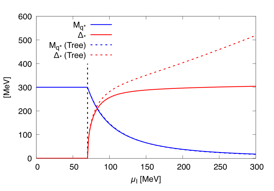
Figure 1: Chiral and pion condensates as functions of a scaled chemical potential $\mu_{I}/m_{\pi}$.

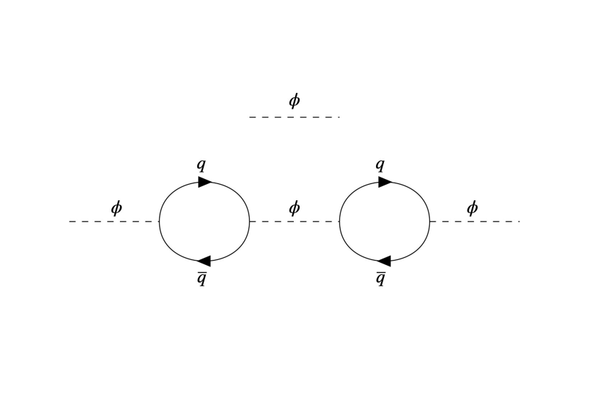
Figure 2: Top: A meson propagator as an elementary particle. Bottom: A meson propagator with a quark loop. The meson can be interpreted as a composite particle.

First we examine how condensates evolve as functions of $\mu_{I}$. Shown in Fig.1 are the constituent quark mass and the gap associated with the pion condensate. For $M_{q}$, there are no significant differences between the tree-level (dashed blue line) and one-loop (solid blue line) results. Meanwhile, the pion condensate $\Delta$ at tree level increases linearly with $\mu_{I}$, whereas, at one-loop, it converges to a finite value, $\Delta\simeq 300\,{\rm MeV}$. This drastic change of behavior indicates that the one-loop correction has more physical contents than mere perturbative corrections.

At tree-level, the Lagrangian makes no reference to quarks so that the mesons are treated as elementary particles (Fig.2 (Top)). By adding quark loops, however, they no longer can be regarded as purely elementary particles. If we regard mesons as fundamental, quark loops are regarded as corrections to the meson dynamics. But if we regard quark descriptions as more fundamental, mesons are intermediate states appearing in the quark-antiquark scattering processes (Fig.2 (Bottom)).

In this study, we keep only the leading $N_{\rm c}$ contributions and hence the quark substructure effects on meson fluctuations are not reflected in EOS (as meson loops are suppressed by $1/N_{\rm c}$). However, the quark substructure effects do affect condensed mesons by tempering the amplitudes. The quark loops change the structure of the present theory and in this sense it may not be appropriate to call quark loops as corrections; rather they should be regarded as leading order contributions.

Now we examine how quark loops qualitatively change the behavior of $\Delta$. To address this question we work with the $\overline{\rm MS}$ expression for the moment as it takes a concise form. We consider a large $\mu_{I}$ and assume $M_{q}\ll\Delta$. At tree level, the effective potential behaves as

$$V_{\rm tree}~{}\rightarrow~{}-\frac{\,2\mu_{I}^{2}\,}{g^{2}}\Delta^{2}+{\lambda\over 24g^{4}}\Delta^{4}\,,$$ (57)

and the solution of the gap equation is found by balancing $\mu^{2}\Delta^{2}$ and $\Delta^{4}$ terms. Hence $\Delta_{\rm tree}\sim\mu_{I}$ inevitably follows. Note also that $\lambda>0$, like the hard core repulsion, plays an essential role to stop the growth of $\Delta$.

Including quark loops, however, the coefficient of $\mu_{I}^{2}$ term acquires the $\ln(\Delta/M_{0})^{2}$ term which, before $\Delta^{4}$ becomes dominant, can stop the growth of $\Delta$. At large $\mu_{I}$ and assuming $\Delta\ll\mu_{I}$,

$$V_{\rm 1-loop}\simeq-2\mu_{I}^{2}\bigg{(}\frac{\,1\,}{\,g^{2}\,}-\frac{\,4N_{\rm c}\,}{\,(4\pi)^{2}\,}\ln\frac{\,\Delta^{2}\,}{\,M_{0}^{2}\,}\bigg{)}\Delta^{2}+V_{q}^{R}\,,$$ (58)

where $V_{q}^{R}\sim\mu_{I}^{4}$ weakly depends upon $\Delta$. Then the gap equation is determined by the coefficient of $\mu_{I}^{2}$ term,

$$\frac{\,\partial V_{\rm 1-loop}\,}{\,\partial\Delta\,}\simeq-\frac{\,8\mu_{I}^{2}N_{\rm c}\,}{\,(4\pi)^{2}\,}\bigg{(}\frac{\,(4\pi)^{2}\,}{\,4g^{2}N_{\rm c}\,}-1-\ln\frac{\,\Delta^{2}\,}{\,M_{0}^{2}\,}\bigg{)}\simeq 0\,.$$ (59)

The solution is $\mu_{I}$-independent,

$$\Delta_{*}^{2}\simeq M_{0}^{2}\,\mathrm{e}^{\frac{\,(4\pi)^{2}\,}{\,4g^{2}N_{\rm c}\,}-1}\,.$$ (60)

For our parameter set, $(4\pi)^{2}/4g^{2}N_{\rm c}\sim 1$ and the exponent is small; we find $\Delta\simeq M_{0}$ as shown in Fig.1.

Substituting the solution into Eq.(58), the $1/g^{2}$ and the logarithmic terms cancel, leaving the $-\mu_{I}^{2}\Delta_{*}^{2}$ term. As a result the pressure $P(\mu_{I})=-V_{\rm 1-loop}(M_{q}^{*},\Delta_{*};\mu_{I})$ has the $+\mu_{I}^{2}\Delta_{*}^{2}$ term,

$$P(\mu_{I})\simeq\frac{\,N_{\rm c}\,}{\,2\pi^{2}\,}\mu_{I}^{2}\Delta_{*}^{2}+P_{q}^{R}(\mu_{I})\,,$$ (61)

where $P_{q}^{R}=-V_{q}^{R}(M_{q}^{*},\Delta_{*})$. The $\mu_{I}^{2}$ dependence can be interpreted as the Fermi surface effects with the phase space $\sim 4\pi p_{F}^{2}$ with $p_{F}$ being the quark Fermi momentum $p_{F}\sim\mu_{I}$.

In this expression for large $\mu_{I}$, hadronic parameters disappear. The hadronic parameters $m^{2}$ and $\lambda$ are neglected because they appear as $m^{2}\Delta^{2}$ and $\lambda\Delta^{4}$ terms much smaller than $\mu_{I}^{2}\Delta^{2}$ and $\mu_{I}^{4}$, while $g^{2}$ is absorbed into the expression of $\Delta_{*}$. The resulting expression can be most naturally understood in terms of quarks with non-perturbative effects near the Fermi surface whose strength depends upon the hadron physics.

III.2 Equations of state

Starting with the thermodyamic pressure $P(\mu_{I})=-V_{\rm 1-loop}(M_{q}^{*},\Delta_{*};\mu_{I})$, the isospin and energy densities are given by

$$n_{I}=\frac{\,\partial P\,}{\,\partial\mu_{I}\,}\,,~{}~{}~{}~{}~{}\varepsilon=\mu_{I}n_{I}-P\,.$$ (62)

We study the sound velocity

$$c_{s}^{2}=\frac{\,\partial P\,}{\,\partial\varepsilon\,}=\frac{\,n_{I}\,}{\,\mu_{I}\chi_{I}\,}\,,~{}~{}~{}~{}~{}\chi_{I}=\frac{\,\partial^{2}P\,}{\,\partial\mu_{I}^{2}\,}\,,$$ (63)

where $\chi_{I}$ is the isospin susceptibility.

In the following we compare our results with the lattice data in Refs. [62] and [63]. The setup of the former is $N_{\rm f}=2+1$ flavors of rooted staggered quarks with the quark masses at the physical point. The pion decay constant is $f_{\pi}\simeq 92$-96 MeV for the lattice spacing explored (the definition of $f_{\pi}$ differs by a factor $\sqrt{2}$ from ours and we have corrected it). It should be noted that their results at $T=0$ are obtained by correcting the data at small but finite $T$ using the ChEFT. Beyond $\mu_{I}\gtrsim m_{\pi}$ or $n_{I}\gtrsim 0.5n_{0}$ the lattice data is not available in Ref. [62]. Meanwhile, the lattice data in Ref. [63] using $m_{\pi}\simeq 170$ MeV and a different formalism is more suitable to explore high density region up to $\mu_{I}\sim 7.5m_{\pi}\simeq 1.3$ GeV (our definition of $\mu_{I}$ is a half of that in Ref. [63], taken into account in our figures).

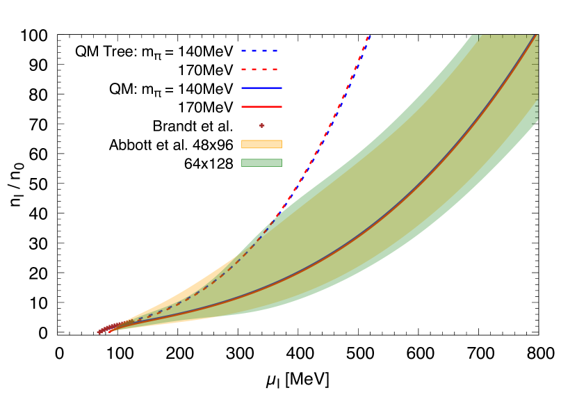
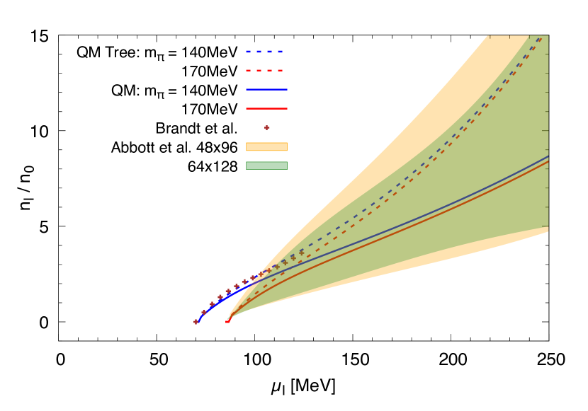
Figure 3: Isospin density $n_{I}$ as a function of $\mu_{I}$, for the global (upper) and low density (lower) behaviors. The data points at low density are from Brandt et al. [62] (available up to $\mu_{I}\simeq 0.9m_{\pi}$ with $m_{\pi}\simeq 140$ MeV) and bands are from Abbott et al. [63] with $m_{\pi}\simeq 170$ MeV. (The definition of $\mu_{I}$ in Ref. [63] differs from ours by a factor 2 and this is taken into account in our figures.)

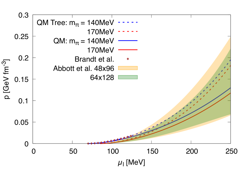
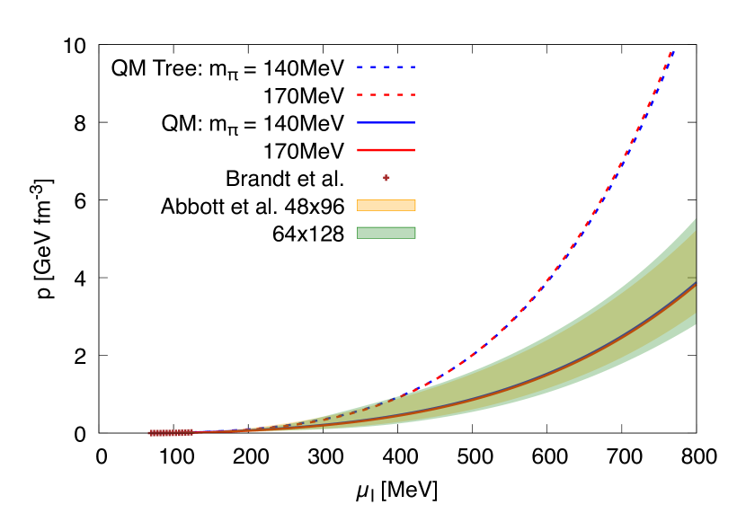
Figure 4: Pressure $P$ as a function of $\mu_{I}$ for the low density (upper panel) and global (lower panel) behaviors.

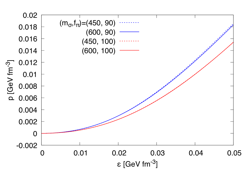
Figure 5: Pressure vs energy density for different $(m_{\sigma},f_{\pi})$ in the MeV unit. Larger chiral symmetry breaking, i.e., larger $m_{\sigma}$ and $f_{\pi}$, reduces the pressure at a given energy density.

Figure 3 shows the isospin density $n_{I}$ as a function of the isospin chemical potential $\mu_{I}$, for the global (upper panel) and low density (lower panel) behaviors. We use $(m_{\sigma},f_{\pi})=(600,90)$ MeV and consider $m_{\pi}=140$ and $170$ MeV for comparison with the lattice data of Refs. [62] and [63]. The upper panel in Fig. 3 is specialized for the examination of global features to high density. As expected from the qualitative difference in the behavior of condensates, the tree and one-loop results become very different toward high density. In purely hadronic descriptions, we found $P\sim\lambda\Delta_{\rm tree}^{4}\sim\lambda\mu_{I}^{4}$ whose asymptotic behavior is controlled by the hadronic coupling $\lambda$, the strength of “hard core repulsion” between mesons. This scaling behaviors are changed by quark loops, with which the scaling $P\sim c\mu_{I}^{4}$ is controlled by the phase space factor for quarks, rather than parameters for hadronic interactions.

In the lower panel of Fig. 3, we make more detailed comparison at low density. We note that the ChEFT results of Ref. [7] including chiral loop corrections agree well with the lattice results of Ref. [62] (see Fig.2 in Ref. [7] for various comparisons), while our model results slightly underestimate $n_{I}$ for a larger $\mu_{I}$. We note that the chiral loops in the ChEFT and quark-loops cover different types of quantum fluctuations. In Fig. 4, we also show the relation between $P$ and $\mu_{I}$ for the low density and global behaviors.

Shown in Fig. 6 is the pressure as a function of energy density. For the density range to $\sim 10n_{0}$, the pressure with quark loops is larger than that that in the tree level by 10-20%. This means that the quark substructure effects enhance the pressure from the purely hadronic one. On the other hand, toward high density the difference in $P$ vs $\varepsilon$ becomes much smaller than in $n_{I}$ vs $\mu_{I}$. Such degeneracy is reached when $P$ enters the $\mu_{I}^{4}$ scaling regime; for whatever coefficients of the $\mu_{I}^{4}$ term, $P\simeq\varepsilon/3$ is achieved when $\mu_{I}^{4}$ terms dominate.

We also note that the pressure is reduced for larger $m_{\sigma}$ and $f_{\pi}$, as shown in Fig. 5. In other words, with stronger chiral symmetry breaking in vacuum (which increases both $m_{\sigma}$ and $f_{\pi}$), the high density EOS after the chiral restoration becomes softer. This point is examined in Sec.IV.1.

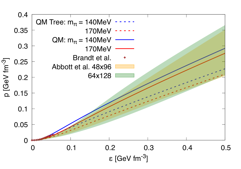
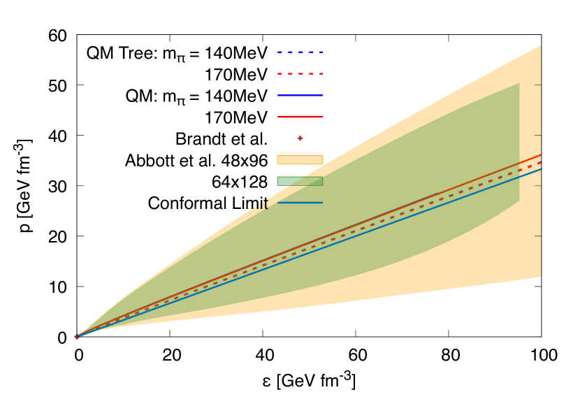
Figure 6: Pressure vs energy density from the tree and one-loop effective potential, for the low density(upper panel) and global (lower panel) behaviors.

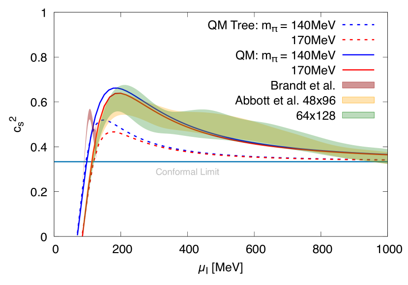
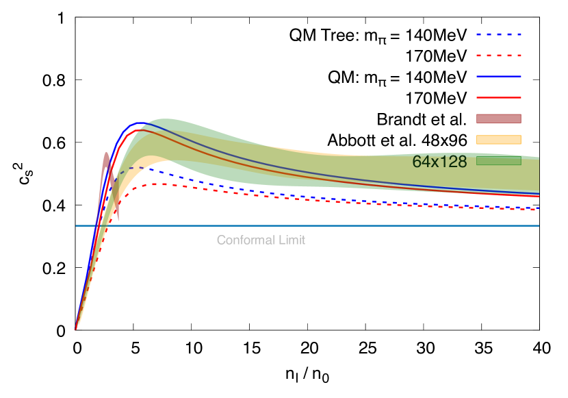
Figure 7: Squared sound velocity $c_{s}^{2}$ vs isospin chemical potential (upper panel) and vs isospin density (lower panel).

To further examine the variation of stiffness, we now turn to the behavior of the sound velocity. Figure 7 shows the $c_{s}^{2}$ as a function of isospin chemical potential and also as a function of isospin density. The $c_{s}^{2}$ increases rapidly at low density, makes a peak, and slowly relaxes to the conformal limit $1/3$ from above. This qualitative feature seems robust and is consistent with the lattice results in Refs. [62] and [63]. However, the quantitative agreement beyond the BEC regime depends on the lattice results. The location of the $c_{s}^{2}$ peak is near $\mu_{I}\simeq 1.2m_{\pi}$ for $n_{I}\simeq 5n_{0}$ in our calculations for the reasonable range of our parameter set for $m_{\sigma}$ and $f_{\pi}$. The lattice results in Ref. [62] indicate the peak at $\mu_{I}\simeq 0.8m_{\pi}$ or $n_{I}\sim 0.5n_{0}$, lower than our model results. Meanwhile our results agree better with the results of Ref. [63], although our sound velocity peak is located at density slightly lower than found in the lattice simulations, 6-7$n_{0}$. We are not sure about the origin of the discrepancy between results of Refs. [62] and [63] as they seem to contain different systematic errors. But after performing several parametric studies as given in Sec. IV, we could not find any qualitative mechanisms to reconcile $\Delta\simeq\Lambda_{\rm QCD}$ with the quick reduction of $c_{s}^{2}$ after making the peak as seen in Ref. [62]. Here we assume $\Delta\simeq\Lambda_{\rm QCD}$ based on the lattice result for the melting temperature of pion condensates, $T_{c}^{\rm lat}\simeq 170$ MeV, which seems more or less constant to $\sim n_{0}$ or even higher densities, see discussions around Eq.(82). For this reason, in the beyond-BEC regime, the results of Ref. [63] seem more natural to us than those of Ref. [62] whose simulations are more optimized for the low density region.

We note that the $c_{s}^{2}$ at tree level also shows the peak in the crossover region and then the convergence to the conformal limit at high density. As we noted in the Introduction, these behaviors can be acheived by $P(\mu_{I})\sim c_{2}\mu_{I}^{2}\Lambda^{2}+c_{4}\mu_{I}^{4}$ with $\Lambda$ being some scale. Purely hadronic models may achieve this condition, but this by itself does not mean that the EOS is described correctly, as we have mentioned in discussion of $P$ vs $\varepsilon$ and $n_{I}$ vs $\mu_{I}$. In our standpoint, the tree level results, which crucially depend on the scaling $\Delta_{\rm tree}\sim\mu_{I}$, becomes potentially misleading at high density.

With the above qualifications in mind, in the next section we look into more details of our model regarding it as a model of composite particles.

III.3 Occupation Probability

At low density the effective degrees of freedom are pions and their internal structure may be ignored. At higher density, the inter particle distance becomes shorter and the quark substructure of pions becomes important.

To estimate where the quark substructure becomes important, we refer to the pion charge radius. It can be extracted from the vector form factor. The experimental determination based on the $\pi e$ scattering and the $e^{+}e^{-}\rightarrow\pi^{+}\pi^{-}$ process [66] yield the estimate $\langle r^{2}\rangle_{V}=0.434(5)\,{\rm fm}^{2}$ [67], or

$$r_{\pi}^{V}=\sqrt{\langle r^{2}\rangle_{V}}~{}\simeq~{}0.66\,{\rm fm}\,,$$ (64)

which has been well reproduced by lattice calculations [68, 69]. The typical isospin density where pions overlap is estimated through

$$n_{I}^{\rm overlap}=2\big{(}4\pi r_{\pi}^{3}/3)^{-1}\simeq 2\times 0.83\,{\rm fm}^{-3}\simeq 10.4n_{0}\,.$$ (65)

Figure 3 shows that the isospin chemical potential at $n_{I}^{\rm overlap}$ is $\mu_{I}\simeq$ 200 MeV $\simeq 1.4m_{\pi}$.

We note that this overlap density $n_{I}^{\rm overlap}\sim 10n_{0}$ is substantially larger than the density 2-3$n_{0}$ where the tree and one-loop results begin to differ substantially, and the density $\sim 5n_{0}$ where $c_{s}^{2}$ develops a peak. This would indicate that the quark substructure of hadrons become important before hadrons overlap. In this respect, there should be a more suitable measure to characterize the location of sound velocity peak. One of possible explanations is the quark saturation [37, 70, 71]. As density increases, quark states at low momentum are inevitably occupied and then a newly added quark must fill a state on top of the already occupied states. Quark states at large momenta are the source of large pressure.

The quark occupation probability in the pion condensed phase can be computed in the standard Nambu-Gor’kov formalism. The derivation is reviewed in Appendix A. The occupation probabilities for $u$-, $d$-, $\bar{u}$-, $\bar{d}$-quarks are

$$f(p)=f_{u,\bar{d}}(p) ={1\over 2}\left(1+{\mu_{I}-E_{D}\over E(\mu_{I})}\right)\,,$$ (66)

$$\bar{f}(p)=f_{\bar{u},d}(p) ={1\over 2}\left(1+{\mu_{I}+E_{D}\over E(\mu_{I})}\right)\,.$$ (67)

Roughly speaking, $u$- and $\bar{d}$-quarks occupy states up to $\simeq\mu_{I}$ while $\bar{u}$- and $d$-quarks are almost fully occupied as in the Dirac sea without pion condensates.

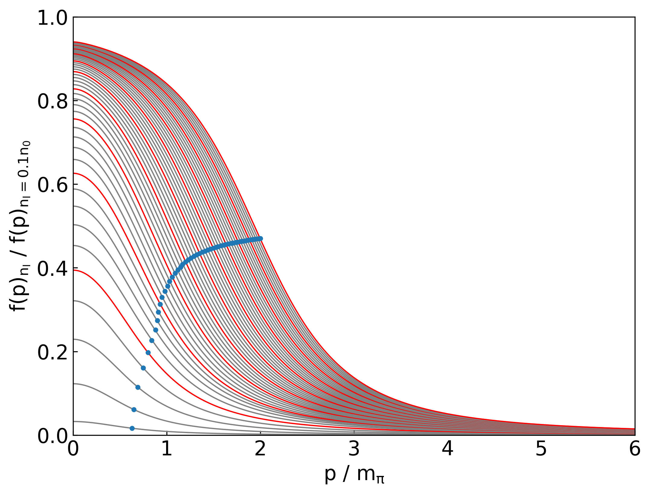
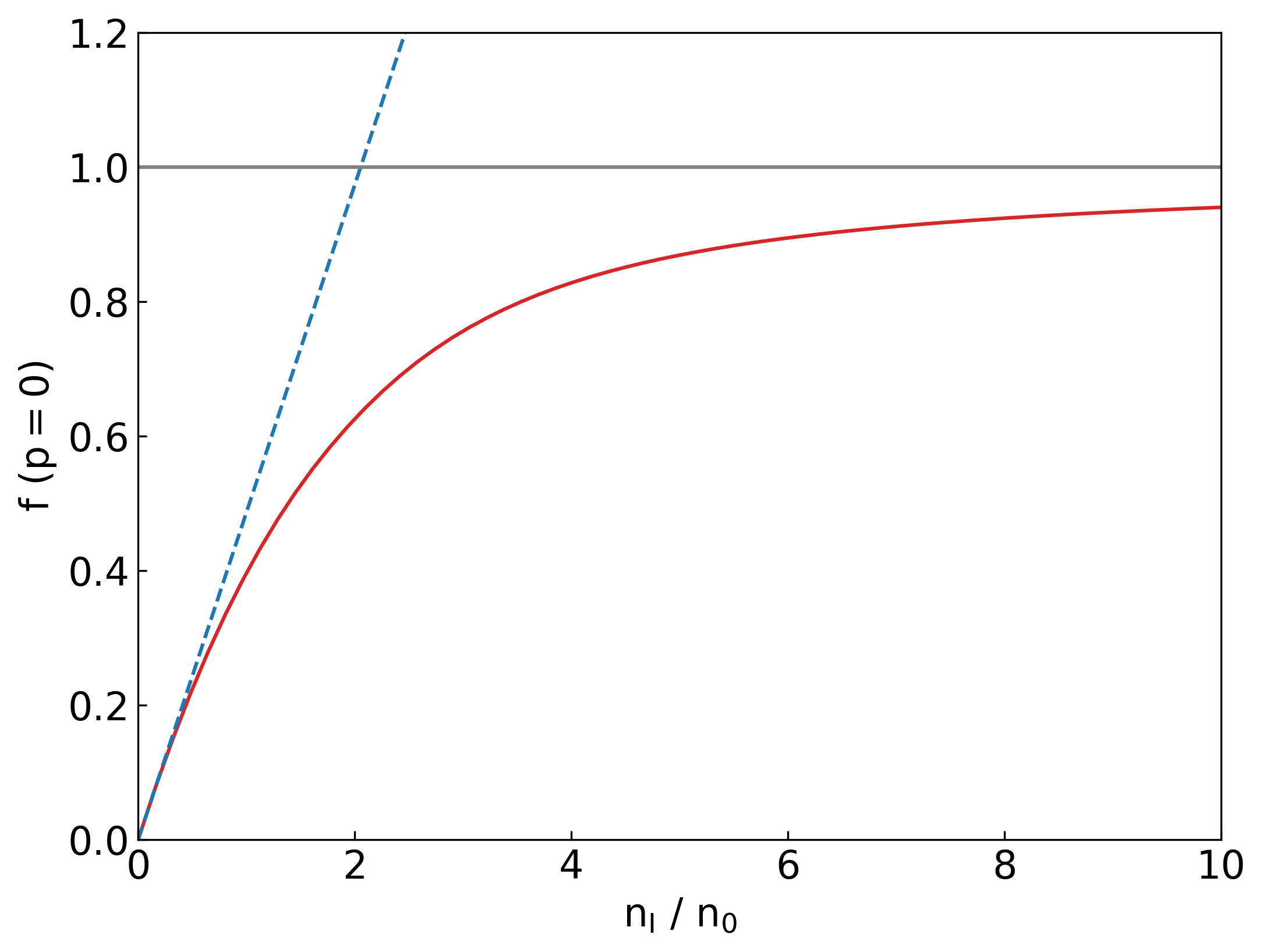
Figure 8: (Upper) The occupation probability of $u$- and $\bar{d}$ quarks which corresponds to the residue of positive energy part of $\langle u\overline{u}\rangle$. The densities we plotted are from $0.2$ to $10.0n_{0}$ in $0.2n_{0}$ increments for gray curves and $1.0n_{0}$ increments for red curves. The blue dots are the locations of the surface of the distribution where $f(p)$ has the half maximum. (Lower) The evolution of the occupation probability for the $p=0$ state, $f(p=0)$.

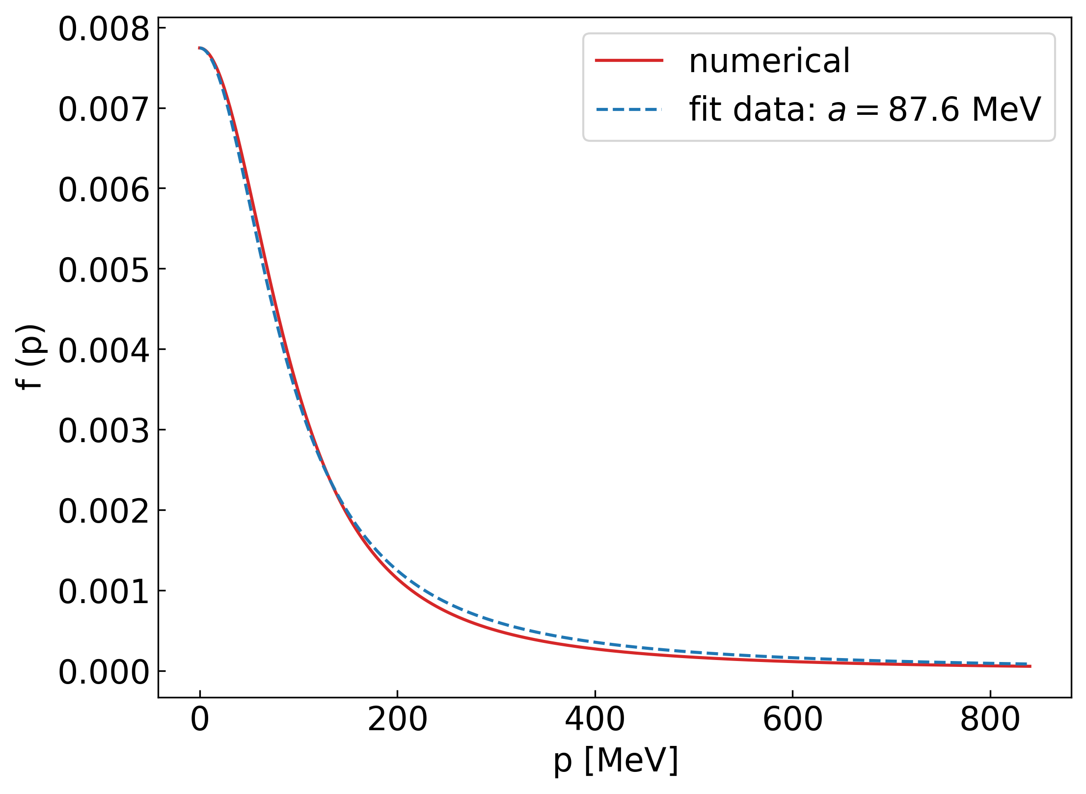
Figure 9: The fit of the dipole function in Eq.(68) to the $\varphi_{\pi}^{\rm vac}$ calculated in the quark-meson model.

Shown in Fig. 9 is the occupation probability $f(p)$ at various densities as a function of quark momenta $p$. The densities we plotted are from $0$ to $10.0n_{0}$ in $0.2n_{0}$ increments for gray curves and $1.0n_{0}$ increments for red curves. The blue dots, where $f(p)$ takes the half value of $f(p=0)$, are the measure of typical momentum at the Fermi surface.

For later convenience we define the quark distribution in a single pion as $\varphi_{\pi}^{\rm vac}(p)\equiv\lim_{n_{I}\rightarrow 0}f(p)/n_{I}$. It turns out that $\varphi_{\pi}^{\rm vac}(p)$ is approximated well by a simple monopole Ansatz or Breit-Wigner form

$$\varphi_{\pi}(p)\sim\frac{1}{\,1+p^{2}/a^{2}\,}$$ (68)

with $a\simeq 87.6$ MeV. This suggests that, in our quark-meson model, the pion wavefunction in the coordinate space has the exponentially-decaying form.

To relate the evolution of $f(p)$ to the stiffening of matter, it is useful to decompose the evolution of $f(p)$ into two components. The first is the “vertical evolution” in which $f(p)$ just increases its magnitude as $f(p)\simeq n_{I}\varphi_{\pi}^{\rm vac}(p)$ (Fig.10, Left); this corresponds to the regime where pions do not interact and quarks inside of pions are largely unaffected. In this regime, $\varepsilon/n_{I}$ is close to a constant, and therefore the pressure, $P=n_{I}^{2}\partial(\varepsilon/n_{I})/\partial n_{I}$, is very small. While quarks can always contribute to the energy density through the masses of pions, they do not directly contribute to the pressure. The sound velocity is small in this regime. The second component is the “horizontal evolution” in which the $f(p)$ increases in the high energy components (Fig.10, Right). This is driven by both interactions and the Pauli blocking effects. Here, $\varepsilon/n_{I}$ increases as in usual quark matter and the pressure can be large. In reality with interactions, the evolution of $f(p)$ is the mixture of these two components.

In our quark-meson model, Fig.9 suggests that, from $0$ to $\sim 2n_{0}$, the magnitude of $f(p)$ at $p=0$ grows rapidly from $0$ to $\simeq 0.6$, but at higher density the distribution $f(p)$ develops toward the horizontal direction. If we treated pions as if elementary and non-ineteracting particles, the $f(p=0)$ would violate the Pauli principle around $\simeq 2n_{0}$. The $c_{s}^{2}$ peak is located around $\simeq 5n_{0}$ where $f(p=0)\simeq 0.9$. Beyond this density the horizontal evolution dominates over the vertical evolution and $c_{s}^{2}$ relaxes toward $1/3$ as in a relativistic quark gas.

We note that, the quark substructure effects are already significant at 1-2$n_{0}$ and develops a peak in $c_{s}^{2}$ at $\sim 5n_{0}$, at density substantially smaller than the naive estimate of the pion overlap, $n_{I}^{\rm overlap}\sim 10n_{0}$. This suggests that the evolution of the occupation probability can represent two characteristic scales; one is for the quark saturation, and the other is for the overlap of composite particles. The distinction of such two scales was emphasized in Ref. [72] which discriminates the mode-by-mode percolation in momentum space from the conventional geometric percolation.

Finally we comment on some difference between nucleonic matter and pionic matter in isospin QCD. In nuclear matter the evolution of $c_{s}^{2}$ is much slower than in isospin QCD, $c_{s}^{2}\lesssim 0.1$ for $n_{B}\sim 1$-$2n_{0}$ [73]. Nucleons are much heavier than pions and $c_{s}^{2}$ is naturally small because of the non-relativistic regime. Two- and three-nucleon repulsions increase $c_{s}^{2}$, but their effects basically enter as powers of $\sim n_{B}^{2}$ and $\sim n_{B}^{3}$ whose growth are rather slow and $c_{s}^{2}$ goes beyond $1/3$ only at $n_{B}\gtrsim$ 2-3$n_{0}$. This aspect differs from pionic matter in isospin QCD where pions can be relativistic already at $\simeq n_{0}$ and $c_{s}^{2}\geq 1/3$ is achieved already at $n_{I}\sim 2n_{0}$.

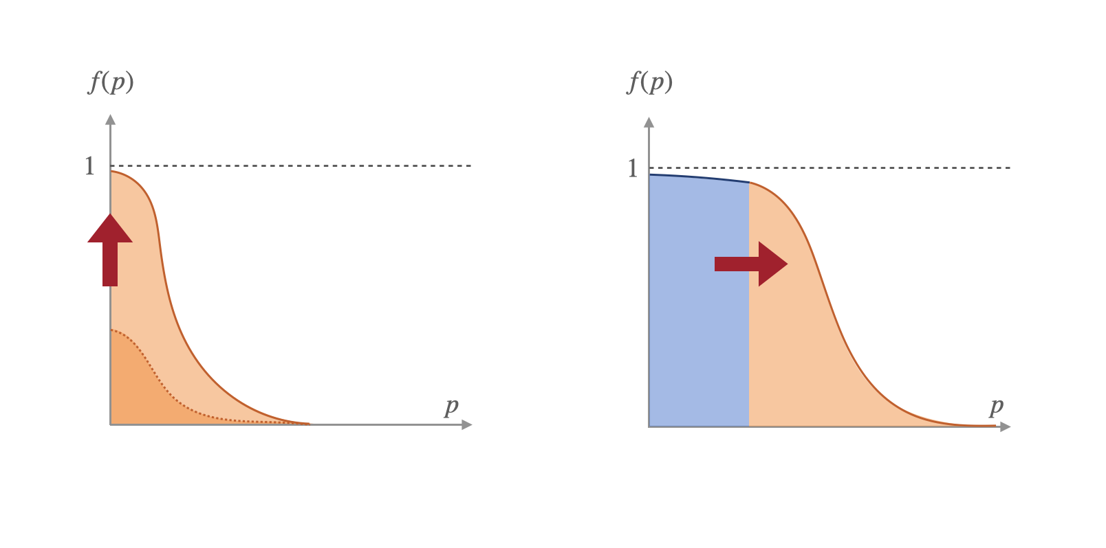
Figure 10: Schematic figures for the evolution of the occupation probability. Left: The “vertical” evolution; Right: The “horizontal” evolution.

IV Discussion

Here we address several issues not detailed in the previous sections. First we discuss how the strength of chiral symmetry breaking in vacuum and its restoration at high density affect EOS. For the high density domain, we compare our results with pQCD at high density, and conjecture the importance of the power corrections. Then we discuss the trace anomaly and the positivity conjecture.

IV.1 Chiral symmetry restoration and softening

In Sec.III we have seen that larger $f_{\pi}$ and/or $m_{\sigma}$ lead to softer EOS at high density. Here we try to explain this softening by focusing on the chiral symmetry breaking in the vacuum and its restoration at high density. In this context larger $f_{\pi}$ and $m_{\sigma}$ mean the stronger chiral symmetry breaking in the QCD vacuum.

In the vacuum, the energy reduction due to the chiral symmetry breaking is (Fig.11)

$$B\equiv V_{\rm 1-loop}(M_{q}=0)-V_{\rm 1-loop}(M_{q}=M_{0})\,,$$ (69)

where the first term is the energy of the trivial vacuum while the second one is the energy of the chiral symmetry broken vacuum. This sort of the energy difference is often called the bag constant. Stronger breaking in the chiral symmetry increases the size of the bag constant (Fig.12). In our model the bag constants $B(m_{\sigma},f_{\pi})$ in the $m_{\pi}^{4}=(140\,{\rm MeV})^{4}\simeq 50.25\,{\rm MeVfm^{-3}}$ unit are given as

$$B(450,90)=0.874,~{}~{}~{}B(450,100)=1.035,$$

$$B(600,90)=1.439,~{}~{}~{}B(600,100)=1.698,$$ (70)

from which one can see that larger $f_{\pi}$ and $m_{\sigma}$, i.e., stronger chiral symmetry breaking, lead to a greater $B$.

A larger bag constant softens EOS at high density. To see this, it is useful to recall a bag model with perturbative corrections. We note that the perturbative expansions are performed around the trivial vacuum. Since our EOS is normalized to make $P=0$ at $\mu=T=0$ for the non-perturbative vacuum, the perturbative evaluation of EOS must be corrected by the non-perturbative normalization constant. Then, the pressure and energy density are

$$P_{\rm pert}^{\rm normalized}=P_{\rm pert}-B,~{}~{}\varepsilon_{\rm pert}^{\rm normalized}=\varepsilon_{\rm pert}+B.$$ (71)

The bag constant associated with the chiral restoration reduces the pressure and increases the energy density, resulting in a softer EoS at high density where the chiral symmetry is restored. Similar conclusions have been obtained in models with and without the $U(1)_{A}$ anomaly [74, 75].

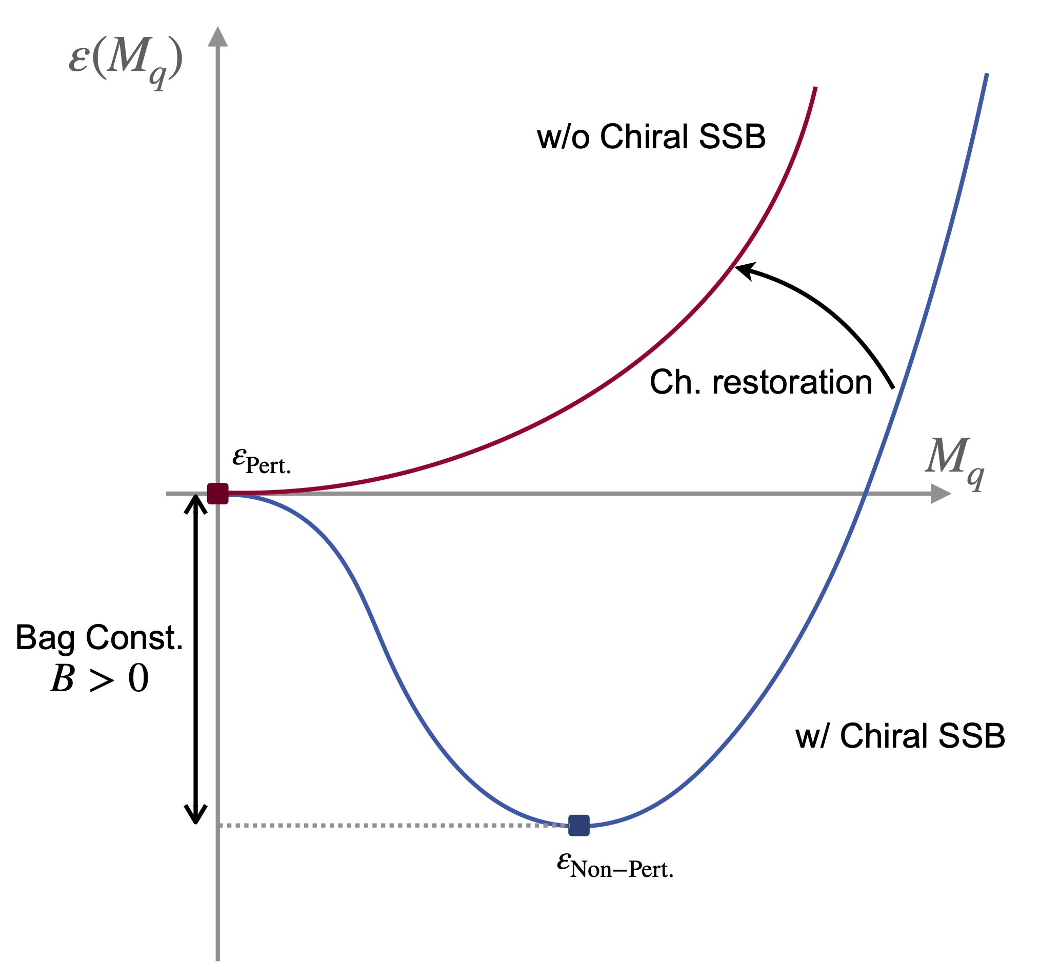
Figure 11: The energy density as a function of the chiral effective mass $M_{q}$. After chiral restoration the minimum energy is realized at $M_{q}=0$. In the broken phase the minimum is realized at $M_{q}\neq 0$ and the energy is smaller than that of $M_{q}=0$. This gap in the zero-point energy density is the bag constant.

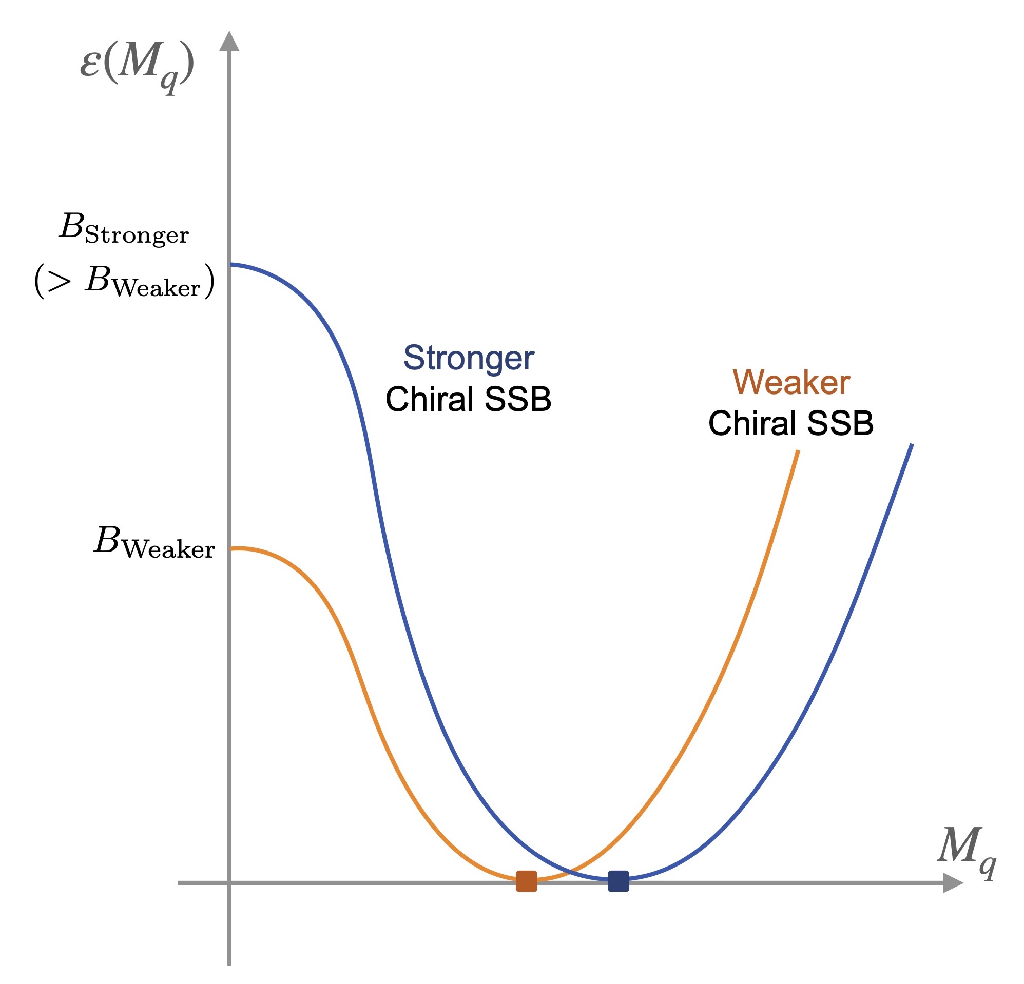
Figure 12: The energy density with different strength of the chiral symmetry breaking. The bag constant is larger for the stronger chiral symmetry breaking.

IV.2 Power corrections to pQCD at high density

Our quark-meson EOS predicts $c_{s}^{2}$ approaching $1/3$ from above as density increases. This contradicts with the pQCD prediction in which $c_{s}^{2}$ approaches $1/3$ from below. A possible origin of such discrepancy would be the power corrections of $\sim\Lambda_{\rm QCD}^{2}\mu_{I}^{2}$ which cannot be derived from perturbative computations.

In Introduction, we schematically showed how power corrections can enhance the $c_{s}^{2}$ in Eqs.(1) and (2). The question is how large power corrections should be to qualitatively change the perturbative behaviors of $c_{s}^{2}$.

For a given flavor $f$, the pQCD EOS up to $O(\alpha_{s}^{2})$ is given as [76] (we use the current quark mass, $m_{u,d}\simeq 5$ MeV and $\mu_{I}=\mu_{u}=-\mu_{d}$ in the present work)

$$P_{0}^{f}\! = \!\frac{N_{\rm c}}{\,12\pi^{2}\,}\bigg{[}|\mu_{f}|u_{f}\bigg{(}\mu_{f}^{2}-\frac{\,5\,}{2}m_{q}^{2}\bigg{)}+\frac{\,3\,}{2}m_{q}^{4}\ln\frac{\,|\mu_{f}|+u_{f}\,}{m_{q}}\bigg{]}\,,$$

$$P_{1}^{f}\! = \!-\frac{\,\alpha_{s}N_{\rm G}\,}{\,16\pi^{2}\,}\bigg{[}3\bigg{(}m_{q}^{2}\ln\frac{\,|\mu_{f}|+u_{f}\,}{m_{q}}-|\mu_{f}|u_{f}\bigg{)}^{2}-2u_{f}^{4}$$

$$+m_{q}^{2}\bigg{(}6\ln\frac{\,\Lambda_{\rm reno}\,}{\,m_{q}\,}+4\bigg{)}\bigg{(}|\mu_{f}|u_{f}-m_{q}^{2}\ln\frac{\,|\mu_{f}|+u_{f}\,}{m_{q}}\bigg{)}\bigg{]}\,.$$

In the isospin symmetric limit, $P^{u}=P^{d}$. Here, $P_{0}^{f}$ and $P_{1}^{f}$ is the zeroth and first order in $O(\alpha_{s})$, with $u_{f}=\sqrt{\mu_{f}^{2}-m_{q}^{2}}$, $N_{\rm G}=N_{\rm c}^{2}-1$, and $\Lambda_{\rm reno}$ being the renormalization scale. The running $\alpha_{s}$ is

$$\alpha_{s}(\Lambda_{\rm reno}) = \frac{\,4\pi\,}{\,\beta_{0}L\,}\bigg{[}1-2\frac{\,\beta_{1}\,}{\,\beta_{0}^{2}\,}\frac{\,\ln L\,}{\,L\,}$$ (73)

$$+ \frac{\,\beta_{1}^{2}\,}{\,\beta_{0}^{4}L^{2}\,}\big{(}\ln^{2}L-\ln L-1+\frac{\,\beta_{2}\beta_{0}\,}{\,\beta_{1}^{2}\,}\big{)}$$

$$+ \frac{\,\beta_{1}^{3}\,}{\,\beta_{0}^{6}L^{3}\,}\big{(}-\ln^{3}L+\frac{\,5\,}{\,2\,}\ln^{2}L+2\ln L$$

$$- \frac{\,1\,}{\,2\,}-3\frac{\,\beta_{2}\beta_{0}\,}{\,\beta_{1}^{2}\,}\ln L+\frac{\,\beta_{3}\beta_{0}^{2}\,}{\,2\beta_{1}^{3}\,}\big{)}\bigg{]}$$

with $L=2\ln(\Lambda_{\rm reno}/\Lambda_{\overline{\rm MS}})$, $\beta_{0}=11-2N_{\rm f}/3$, $\beta_{1}=102-19N_{\rm f}/3$,

$$\beta_{2}\! = \!\frac{\,2857\,}{\,2\,}-\frac{\,5033\,}{\,18\,}N_{f}+\frac{\,325\,}{\,54\,}N_{f}^{2}\,,$$ (74)

$$\beta_{3}\! = \!\bigg{(}\frac{\,149753\,}{\,6\,}+3564\,\xi(3)\bigg{)}$$ (75)

$$\!-\bigg{(}\frac{\,1078361\,}{\,162\,}+\frac{\,6508\,}{\,27\,}\xi(3)\bigg{)}N_{f}$$

$$\!+\bigg{(}\frac{\,50065\,}{\,162\,}+\frac{\,6472\,}{\,81\,}\xi(3)\bigg{)}N_{f}^{2}$$

$$\!+\frac{\,1093\,}{\,729\,}N_{f}^{3}$$

and $\Lambda_{\overline{\rm MS}}\simeq 340\,{\rm MeV}$. The central value of $\Lambda_{\rm reno}$ is $\Lambda_{\rm reno}=\mu_{f}$, and as usual we vary $\Lambda_{\rm reno}$ from $\mu_{f}$ to $4\mu_{f}$.

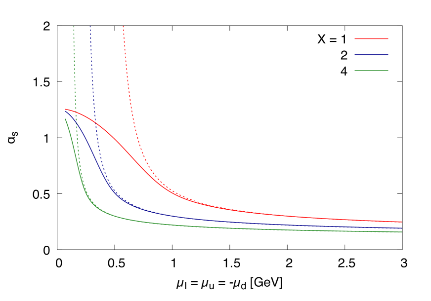
Figure 13: Running coupling from pQCD (dashed) and from the freezing coupling (solid). For the renormalization scale $\Lambda_{\rm reno}=X\mu_{I}$, we examine $X=1,2$, and $4$.

In addition to the perturbative running coupling which becomes unphysical toward the Landau pole, we also examine the case with the freezing coupling in the low energy limit. We divide the domain into three

$$\alpha_{s}(Q^{2}) = \alpha^{\rm low}_{s}(Q^{2})\theta(t_{\rm low}-Q^{2})$$ (76)

$$+ \alpha^{\rm mid}_{s}(Q^{2})\theta(t_{\rm high}-Q^{2})\theta(Q^{2}-t_{\rm low})$$

$$+ \alpha^{\rm high}_{s}(Q^{2})\theta(Q^{2}-t_{\rm high})\,.$$

where $t_{\rm low}^{1/2}=0.3\,{\rm GeV}$ and $t_{\rm high}^{1/2}=1.1$ GeV. For the low energy limit we use the form suggested by Deur et al [77, 78]

$$\alpha_{s}^{\rm low}=\alpha_{s}^{\rm low}(0)\mathrm{e}^{-Q^{2}/4\kappa^{2}}\,,$$ (77)

with $\alpha_{s}^{\rm low}(0)\simeq 1.22$ and $\kappa\simeq 0.51$. For the high density we use the perturbative expression (73), and for the intermediate region we use the interpolant

$$\alpha_{s}^{\rm mid}(Q^{2})=\sum_{m=0}^{5}c_{m}\mu_{I}^{m}\,,$$ (78)

where $c_{n}$’s are fixed by demanding the matching

$$\frac{\,\partial^{n}\alpha_{s}^{\rm low/high}}{(\partial Q^{2})^{n}}\bigg{|}_{Q^{2}=t_{\rm low/high}}=\frac{\,\partial^{n}\alpha_{s}^{\rm mid}}{(\partial Q^{2})^{n}}\bigg{|}_{Q^{2}=t_{\rm low/high}}\,,$$ (79)

for $n=0,1,2$. The six boundary conditions fix the six $c_{n}$ uniquely. Unlike in Refs. [77, 78] which needed only the continuity up to the first derivative, in this work we use the interpolant not to generate any discontinuities up to the second derivative, since we compute $c_{s}^{2}$.

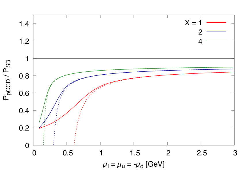
Figure 14: Perturbative pressure with perturbative running with the Landau pole and infrared freezing coupling. The pressure is normalized by the pressure in the Stefan-Boltzmann limit. Notations for the solid and dashed lines are the same as Fig. 13.

We set $Q^{2}=\Lambda_{\rm reno}^{2}$ and plot $\alpha_{s}(\Lambda_{\rm reno})$ in Fig.13 together with the pQCD running coupling. With the IR freezing coupling the artificial reduction of pQCD pressure is tempered and the pressure remains positive toward the low density region (Fig.14).

Now we add power corrections which are parametrized in terms of gaps in the pion condensed phase. The phase space factor $\sim 4\pi p_{F}^{2}\Delta$ times the gap $\Delta$, divided by a factor $(2\pi)^{3}$, yields the naive estimate

$$P_{\rm cond}=C\frac{\,\mu_{I}^{2}\Delta^{2}\,}{\,\pi^{2}\,}\,,$$ (80)

where $C$ is a constant of $O(1)$. For our quark meson model $C\simeq N_{\rm c}/2$, see Eq. (61).

In Son’s estimate [79], based on the color-magnetic long range forces, the gap is evaluated as

$$\Delta_{\rm color-mag}=b|\mu_{I}|g_{s}^{-5}\mathrm{e}^{-3\pi^{2}/2g_{s}}$$ (81)

with $b\sim 10^{4}$ and $g_{s}=g_{s}(|\mu_{I}|)$ being the running coupling constant. The gap can be several hundreds MeV. Meanwhile, in our quark-meson model, we have found $\Delta\simeq 300$ MeV. It is interesting to note that such $\Delta$ seems to satisfy the BCS relation between the gap and the critical temperature,

$$T_{c}^{\rm BCS}\simeq 0.57\,\Delta_{\rm BCS}\,,$$ (82)

which implies $T_{c}\simeq 171\,{\rm MeV}$, in good agreement with the lattice result $T_{c}^{\rm lattice}\simeq 160$-$170\,{\rm MeV}$ for the interval $\mu_{I}\simeq 100$-$300\,{\rm MeV}$.

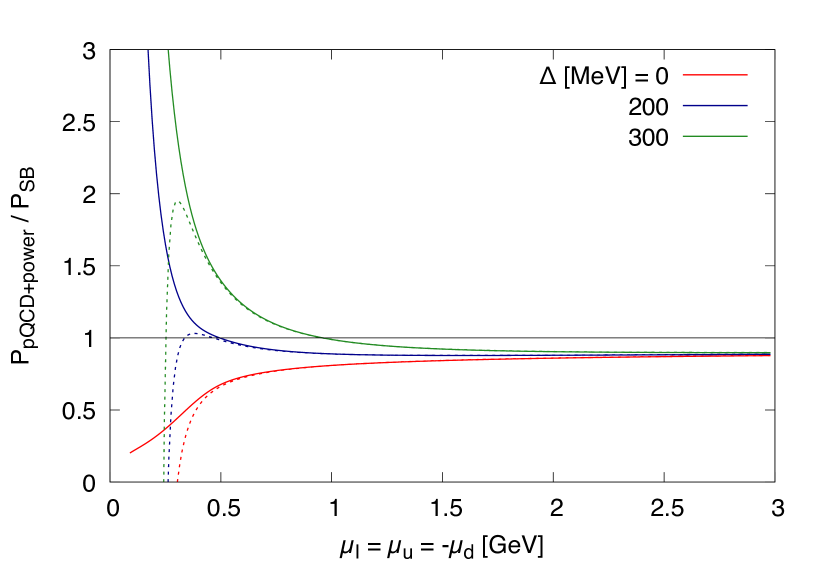
Figure 15: Perturbative pressure plus power corrections divided by the pressure in the Stefan-Boltzmann limit. The $\Delta=0,200$, and $300$ MeV. The solid and dashed lines represent the freezing coupling and perturbative running with the Landau pole, respectively. The $X$ for the $\Lambda_{\rm reno}$ is fixed to $X=2$.

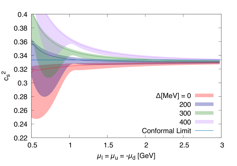
Figure 16: Squared sound velocity $c_{s}^{2}$ for pQCD+power corrections. We use the freezing coupling and vary $X$ from $1$ to $4$ to make bands. The solid lines in the bands are the $X=2$ case.

We set $C=1$ and examine pressure (Fig. 15) and $c_{s}^{2}$ (Fig. 16) for $\Delta=0,200$, and $300$ MeV for pQCD running coupling (dashed) and freezing coupling (solid). For $\Delta\simeq 200$ MeV, the power corrections are large enough for $c_{s}^{2}$ to approach the conformal limit from above around $\sim 40n_{0}$. Meanwhile, at $\mu_{I}\sim 1$ GeV or $n_{I}\sim 40n_{0}$, parametrically the power corrections in EOS are corrections of the order

$$\bigg{(}\frac{\,\Delta\,}{\,\mu_{I}\,}\bigg{)}^{2}=0.09\bigg{(}\frac{\,\Delta\,}{\,300\,{\rm MeV}\,}\bigg{)}^{2}\bigg{(}\frac{\,1\,{\rm GeV}\,}{\,\mu_{I}\,}\bigg{)}^{2}\,,$$ (83)

thus $\sim 10\%$ corrections. It is remarkable that even such small corrections can change the qualitative behaviors of $c_{s}^{2}$ in the domain where pQCD seems applicable.

IV.3 Trace Anomaly

Recently there has been growing interest in the trace anomaly in the context of mechanical properties in hadrons [72, 80, 81, 82] and in neutron stars [48, 49, 50]. The latter is essentially the relation between $P$ vs $\varepsilon$ and is more fundamental than $c_{s}^{2}$ which includes only the information of $\mathrm{d}P/\mathrm{d}\varepsilon$, not the overall magnitude of $P$. In particular, Ref. [49] conjectured the trace anomaly to be positive. Below we quickly mention the trace anomaly in dense matter and examine the positivity conjecture by considering several non-perturbative effects.

The trace anomaly measures the breaking of the scale invariance and is given by the expectation values of the operator

$$\partial_{\mu}J^{\mu}_{D}=T^{\mu}_{\mu}=-\frac{\,\beta(g_{s})\,}{2g_{s}}G^{\mu\nu}G_{\mu\nu}+\sum_{f}m_{f}(1+\gamma_{m})\bar{q}_{f}q_{f}\,,$$

where $J^{\mu}_{D}$ is the dilatation current, $\beta<0$ the QCD beta function, and $\gamma_{m}$ the anomalous dimension of the quark mass.

For a hadronic state $|K\rangle$ with the momentum $K$, the energy momentum tensor gives

$$\langle K|T^{\mu\nu}(x)|K\rangle=K^{\mu}K^{\nu}/m_{H}\,,$$ (85)

where the RHS is $x$-independent and does not contain $g^{\mu\nu}$. The overall $1/m_{H}$ factor is fixed by the condition at the rest frame, $K_{R}^{\mu}=(m_{H},{\bf 0})$,

$$\frac{\,\langle K_{R}|H|K_{R}\rangle\,}{\,\langle K_{R}|K_{R}\rangle\,}=\frac{\,\langle K_{R}|\int_{\bm{{x}}}T^{00}(x)|K_{R}\rangle\,}{\,\langle K_{R}|K_{R}\rangle\,}=m_{H}\,,$$ (86)

where we divide by $\langle K_{R}|K_{R}\rangle$ to cancel the volume factor in the numerator. Thus, for a hadron at rest frame, we find

$$\langle K_{R}|T^{\mu}_{\mu}(x)|K_{R}\rangle=\langle K_{R}|T^{00}(x)|K_{R}\rangle=m_{H}\,,$$ (87)

with vanishing spatial components, $\langle K_{R}|T^{ii}(x)|K_{R}\rangle=0$. The trace anomaly is positive for a single hadron.

It is interesting to extend the above arguments to a many-body system. Unlike the previous single particle case, not all particles stay at ${\bm{K}}=0$. For instance an ideal Fermi gas leads to

$$\langle K_{1},\cdots|T^{ii}|K_{1},\cdots\rangle\sim\int_{{\bm{K}}}\frac{\,{\bm{K}}^{2}\,}{\,m_{H}\,}\,.$$ (88)

After lowering one index, we get $\langle T^{i}_{i}\rangle<0$. Thus, the trace anomaly in a many-body system can be negative in principle. In thermodynamic systems, $\langle T^{\mu}_{\mu}\rangle=\varepsilon-3P$; the negative trace anomaly means very large pressure, i.e., stiff EOS.

The trace anomaly characterizes the deviation from the relativistic or conformal limit as expected at very high density. We first examine the impact of the normalization in EOS. In the case of a bag model, we have

$$\langle T^{\mu}_{\mu}\rangle_{\rm bag}=\big{(}\varepsilon-3P\big{)}_{\rm pert}^{\rm normalized}=\big{(}\varepsilon-3P\big{)}_{\rm pert}+4B\,.$$ (89)

Changes from the non-perturbative to perturbative vacua enhances the trace anomaly, supporting the positivity conjecture. Next we consider the impact of power corrections using EOS similar to Eq.(1),

$$P_{\rm with\,powers}=a_{0}\mu_{I}^{4}+a_{2}\mu_{I}^{2}\,,$$ (90)

but now we include the running of coefficients $a_{0}$ and $a_{2}$ associated with $\alpha_{s}(\mu_{I})$. The energy density can be computed as

$$\varepsilon=3a_{0}\mu_{I}^{4}+2a_{2}\mu_{I}^{2}+\frac{\,\partial a_{0}\,}{\,\partial\ln\mu_{I}\,}\mu_{I}^{4}+\frac{\,\partial a_{2}\,}{\,\partial\ln\mu_{I}\,}\mu_{I}^{2}\,,$$ (91)

and the trace anomaly is

$$\langle T^{\mu}_{\mu}\rangle_{\rm with\,powers}=-2a_{2}\mu_{I}^{2}+\frac{\,\partial a_{0}\,}{\,\partial\ln\mu_{I}\,}\mu_{I}^{4}+\frac{\,\partial a_{2}\,}{\,\partial\ln\mu_{I}\,}\mu_{I}^{2}\,.$$ (92)

The running of $\alpha_{s}$ favors the positive trace anomaly, while the attractive power corrections ($a_{2}>0$) favor the negative trace anomaly.

When we examine the trace anomaly, it is useful to divide it by $3\varepsilon$,

$$\Delta_{\rm tr}=\frac{\,1\,}{\,3\,}-\frac{\,P\,}{\,\varepsilon\,}\,,$$ (93)

which should not be confused with the BCS gap $\Delta$. Shown in Fig.17 is the $\Delta_{\rm tr}$ as functions of $n_{I}$ for several calculations, our quark meson model (QM) and pQCD results for the renormalization scales with $X=1,2$, and $4$. For the pQCD, both the perturbative (dashed) and IR freezing (solid) couplings are examined. Without power corrections the $\Delta_{\rm tr}$ are all positive. In Fig.18, we fix $X=2$ for these two couplings, and the dependence of $\Delta_{\rm tr}$ on the power corrections. The $\Delta=0,200,300$, and $400$ MeV cases are shown. With power corrections the $\Delta_{\rm tr}$ appears to be negative, as we expected. Our QM model predicts $\Delta\simeq 300$ MeV and the negative trace anomaly for wide range. Finally we make a comparison between our QM model results and the lattice results in Ref. [63], as shown in Fig. 19. The QM model seems to capture the overall trend of the lattice data.

Since the pQCD corrections and bag constant favor the positive $\Delta_{\rm tr}$, the negative $\Delta_{\rm tr}$ may be taken as an indicator of the substantial power corrections.

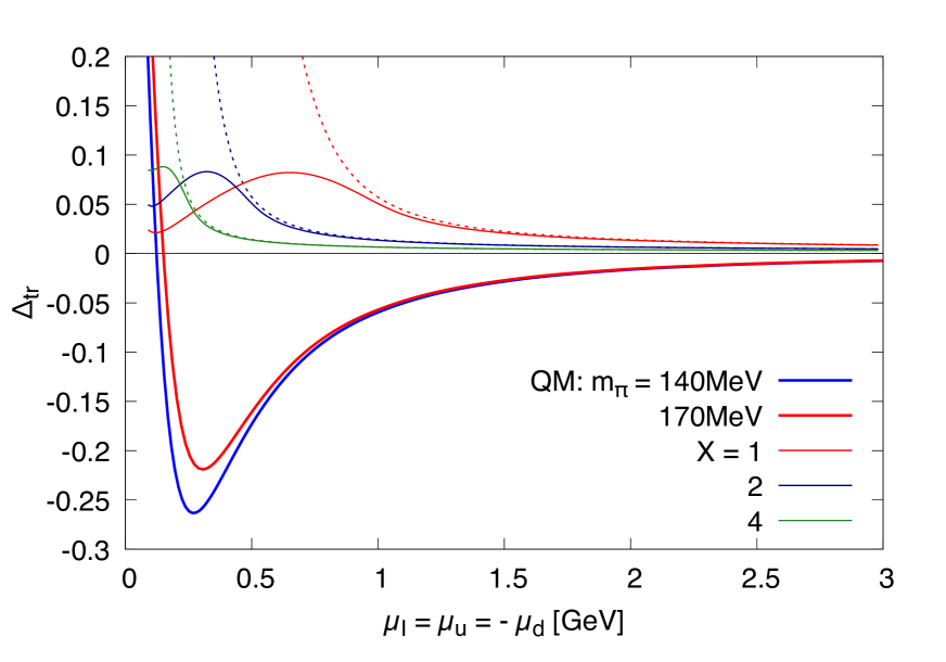
Figure 17: Trace anomaly $\Delta_{\rm tr}=1/3-P/\varepsilon$ as functions of $n_{I}$ for our quark-meson model ($N_{\rm f}=2$ QM) and pQCD with the perturbative running coupling (dashed) and IR freezing coupling (solid). We vary $X$ from 1 to 4. The trace anomaly is all positive in pQCD but negative for the quark meson model.

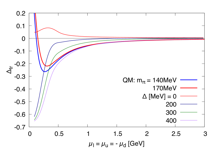
Figure 18: Trace anomaly $\Delta_{\rm tr}=1/3-P/\varepsilon$ as functions of $n_{I}$ for the quark-meson model, the pQCD + powers with the perturbative running. The renormalization scale is fixed to $X=2$ while we examine $\Delta=0,200,300,400$ MeV. For large $\Delta$ the trace anomaly can be negative.

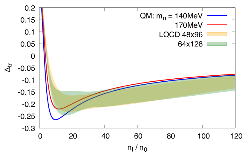
Figure 19: Trace anomaly $\Delta_{\rm tr}=1/3-P/\varepsilon$ as functions of $\mu_{I}/m_{\pi}$ for the quark-meson model with $m_{\pi}=140,170$ MeV and lattice results of Ref. [63] with $m_{\pi}\simeq 170$ MeV for different lattice spacing and volume.

V Summary

In this work we study the EOS of isospin QCD within a quark-meson model. The model describes the BEC-BCS crossover of pion condensates. At tree level pions look elementary, but at one-loop they acquire the status of composite particles made of quarks and anti-quarks, tempering meson fields compared to the tree level amplitudes. The model is renormalizable and we study its large density behaviors to study the impacts of non-perturbative physics in the quark matter domain.

Our model exhibits the sound velocity going beyond the conformal limit $c_{s}^{2}=1/3$ at $\sim 2n_{0}$, and making a peak at $\sim 5n_{0}$, at densities substantially smaller than the density for pions to spatially overlap, $\sim 10n_{0}$. The quark occupation probability at $p=0$, $f(p=0)$, is $\sim 0.6$ at $2n_{0}$ and $\sim 0.9$ at $5n_{0}$. The sound velocity peak is located around $5n_{0}$ where the quark states around $p=0$ are almost fully saturated, and it makes sense to associate the sound velocity peak with the saturation of quark states. After the bulk part of the quark Fermi surface is established, the $c_{s}^{2}$ approaches $1/3$ as in the relativistic limit.

Our model shows that $c_{s}^{2}$ approaches 1/3 from above, mainly due to the power corrections, $\sim\mu_{I}^{2}\Delta^{2}\sim\mu_{I}^{2}\Lambda_{\rm QCD}^{2}$. This sort of terms is not available in pQCD calculations which predict $c_{s}^{2}$ approaching $1/3$ from below. Which one, perturbative or power corrections, dominates in $c_{s}^{2}$ around $\sim 40n_{0}$ is a quantitative question. The existence of the power corrections is related to the non-perturbative effects near the quark Fermi surface and the structure of the QCD phase diagram. The question is also related to the sign of the trace anomaly. The pQCD favors the positive trace anomaly. If the trace anomaly appears to be negative, it is strong indication of nontrivial Fermi surface structure. Lattice results of Ref. [63] seem to support the negative trace anomaly in the domain between the BEC and the pQCD domains. Since the presence of non-perturbative effects in quark matter is a fundamental question, further clarifications by several lattice calculations with different systematics are highly desired to establish the findings in Ref. [63].

The present work left several issues and should be extended to several directions:

i) Our study should be extended to finite temperature (for recent discussions on the quark contributions, see e.g., Refs. [83, 84]). Including thermal effects into quark-meson models is straightforward, and the results are to be compared with the lattice’s. Whether thermal excitations out of the quark Fermi sea are confined or deconfined is an important issue in the context of the quark-hadron-continuity. As for phenomenological applications to neutron stars and heavy-ion-collisions, although several zero temperature EOS have become available since 2012, finite temperature EOS with the continuity at the level of excitations has not been constructed. For example, some difficulties have been addressed for the nuclear-2SC continuity in Ref. [85]. The magnitude of thermal corrections is much smaller than the cold matter part due to $\sim(T/p_{F})^{2}$ suppression factors, but it can be important for NSs about to collapse, e.g., those appearing in NS-NS mergers [86, 87, 88].

ii) The estimate of non-perturbative power corrections as well as the normalization of EOS (bag constant) at high density should be improved. Nowadays there has been increasing use of pQCD results to constrain the EOS at $\simeq 5$-$40n_{0}$, with the help of general causality and thermodynamic stability conditions (e.g., see Refs. [53, 89]). But as seen in our simple exercise in Sec.IV.2, the power corrections of $\sim 10$% in the overall magnitude can change the qualitative trend of quantities involving derivatives. It should be important to see how the power corrections in general affect the constraints at $\simeq 5$-$40n_{0}$. The present one-loop analyses of quark-meson models should be also improved, using e.g., the functional renormalization group to include quark and meson fluctuations [90].

iii) In this work we estimate the density for pion overlap based on the size of pions in vacuum. But in medium pions may swell due to the quark exchange among them. If the effective radii are larger than in the vacuum, the quark saturation and the overlap of pions can take place at lower densities than the estimates in this work. Changes in hadron size may occur already around nuclear saturation density [91, 92], as indicated by the comparison of the structure function for an isolated nucleon and nucleons in nuclei. It is interesting to test these concepts in isospin QCD by comparing model predictions with the lattice calculations.

Appendix A Quark propagators

We calculate the mean field quark propagator in the presence of the chiral and pion condensates. From the propagator one can read off the excitation energy from the pole of the propagator and the occupation probability from the residue of the propagator.

It is convenient to introduce the projection operators for particle and antiparticles,

$$\Lambda_{p,a}={1\over 2}\pm{\gamma_{j}p^{j}+M_{q}\over 2E_{D}}\gamma_{0}\,,$$ (94)

which satisfy

$$\Lambda_{p}+\Lambda_{a}=1\,,~{}\Lambda_{p,a}\Lambda_{p,a}=\Lambda_{p,a}\,,~{}\Lambda_{p,a}\Lambda_{a,p}=0\,,$$ (95)

as they should. The propagator of quarks can be written as

$${\mathrm{i}\over{\ooalign{\hfil/\hfil\crcr$p$}}+\mu_{f}\gamma_{0}-M_{q}} = S_{p}(p)\gamma_{0}\Lambda_{p}+S_{a}(p)\gamma_{0}\Lambda_{a}\,,$$ (98)

$$S_{p,a}(p) = {\mathrm{i}\over p_{0}+\mu_{f}\mp E_{D}}\,,$$ (99)

where $S_{p,a}$ is the propagator for a particle and an antiparticle, respectively.

The inverse of the propagator can also be separated by $\Lambda_{p,a}$ as

$${\ooalign{\hfil/\hfil\crcr$p$}}+\mu_{f}\gamma_{0}-M_{q} = (p_{0}+\mu_{f}-E_{D})\Lambda_{p}\gamma_{0}$$ (103)

$$+(p_{0}+\mu_{f}+E_{D})\Lambda_{a}\gamma_{0}\,.$$

The inverse of the Dirac operator is the quark propagator $S(p)$, and we can write

$$S(p)^{-1}\equiv-\mathrm{i}\left(\begin{matrix}{\ooalign{\hfil/\hfil\crcr$p$}}+\mu_{u}\gamma_{0}-M_{q}&-i\gamma_{5}\Delta\\ -i\gamma_{5}\Delta&{\ooalign{\hfil/\hfil\crcr$p$}}+\mu_{d}\gamma_{0}-M_{q}\end{matrix}\right)$$ (104)

and consider its inverse. To simplify the discussion, we introduce the single-particle propagator

$$(G_{u,d}^{0})^{-1}=-\mathrm{i}\left({\ooalign{\hfil/\hfil\crcr$p$}}+\mu_{u,d}\gamma_{0}-M_{q}\right)\,,$$ (107)

and write off-diagonal term $\Xi=\gamma_{5}\Delta$. Then our propagator must satisfy

$$S(p)^{-1}S(p)=\left(\begin{matrix}(G_{u}^{0})^{-1}&\Xi\\ \Xi&(G_{d}^{0})^{-1}\end{matrix}\right)S(p)={\bf 1}.$$ (108)

Introducing $(G_{u,d})^{-1}\equiv(G_{u,d}^{0})^{-1}-\Xi G_{d,u}^{0}\Xi$, the propagator $S(p)$ can be written as follows.

$$S(p)=\left(\begin{matrix}G_{u}&-G_{u}^{0}\Xi G_{d}\\ -G_{d}^{0}\Xi G_{u}&G_{d}\end{matrix}\right).$$ (109)

What we are interested in is the diagonal part of $S(p)$ which corresponds to $\langle u\overline{u}\rangle$ and $\langle d\overline{d}\rangle$. Let us see the detail of $G_{u,d}$. Its definition is

$$(G_{u,d})^{-1}\equiv(G_{u,d}^{0})^{-1}-\Xi G_{d,u}^{0}\Xi$$

$$=-\mathrm{i}\left({\ooalign{\hfil/\hfil\crcr$p$}}+\mu_{u,d}\gamma_{0}-M_{q}\right)-\gamma_{5}\Delta{\mathrm{i}\over{\ooalign{\hfil/\hfil\crcr$p$}}+\mu_{d,u}\gamma_{0}-M_{q}}\gamma_{5}\Delta\,.$$ (114)

To calculate the inverse we rewrite this formula using the projection operators. Performing some calculations we can find

$$\gamma_{5}\gamma_{0}\Lambda_{p,a}\gamma_{5}=-\Lambda_{a,p}\gamma_{0}.$$ (116)

From the above, we obtain

$$(G_{u,d})^{-1} = -\mathrm{i}\bigg{[}{\,p_{0}^{2}-(E_{D}-\mu_{u,d})^{2}-\Delta^{2}\over p_{0}-\mu_{u,d}+E_{D}}\Lambda_{p}\gamma_{0}$$ (117)

$$~{}+\,{\,p_{0}^{2}-(E_{D}+\mu_{u,d})^{2}-\Delta^{2}\over p_{0}-\mu_{u,d}-E_{D}}\Lambda_{a}\gamma_{0}\bigg{]}.$$

Now we could separate the diagonal elements $(G_{u,d})^{-1}$ by projection operators, and each part will not be mixed by the inverse operation.

Introducing the excitation energy

$$\xi_{p,a}^{f}(p)=\sqrt{(E_{D}\mp\mu_{f})^{2}+\Delta^{2}},$$ (118)

we obtain the propagator

$$G_{f} = \mathrm{i}\bigg{[}{|u_{p}^{f}(p)|^{2}\over\,p_{0}-\xi_{p}^{f}(p)}+{|v_{p}^{f}(p)|^{2}\over\,p_{0}+\xi_{p}^{f}(p)}\bigg{]}\gamma_{0}\Lambda_{p}$$ (119)

$$+ \mathrm{i}\bigg{[}{|u_{a}^{f}(p)|^{2}\over\,p_{0}-\xi_{a}^{f}(p)}+{|v_{a}^{f}(p)|^{2}\over\,p_{0}+\xi_{a}^{f}(p)}\bigg{]}\gamma_{0}\Lambda_{a}\,.$$

Here we have used $\mu_{u,d}=-\mu_{d,u}$. The residues are

$$|u_{p,a}^{f}(p)|^{2} ={1\over 2}\left(1+{\pm E_{D}-\mu_{f}\over\xi_{p,a}^{f}}\right)$$ (120)

$$|v_{p,a}^{f}(p)|^{2} ={1\over 2}\left(1-{\pm E_{D}-\mu_{f}\over\xi_{p,a}^{f}}\right).$$ (121)

They correspond to the occupation probability and satisfy $|u_{p}|^{2}+|v_{p}|^{2}=|u_{a}|^{2}+|v_{a}|^{2}=1$ as expected. In the main text we use the expressions

$$f=f_{u,\bar{d}} ={1\over 2}\left(1+{\mu_{I}-E_{D}\over E(\mu_{I})}\right)=|v_{p}^{u}|^{2}=|u_{a}^{d}|^{2}\,,$$ (122)

$$\bar{f}=f_{\bar{u},d} ={1\over 2}\left(1+{\mu_{I}+E_{D}\over E(\mu_{I})}\right)=|v_{a}^{u}|^{2}=|u_{p}^{d}|^{2}\,.$$ (123)

Appendix B Full expression of the renormalized one-loop effective potential

In the main text we express the one-loop effective potential using several counter terms. Rewriting the counter terms using the physical parameters, the final expression turns out to be

$$V_{\rm 1-loop} =-\frac{1}{\,4\,}m_{\sigma}^{2}f_{\pi}^{2}\bigg{[}1+\frac{4M_{0}^{2}N_{\rm c}}{\,(4\pi)^{2}f_{\pi}^{2}\,}\bigg{\{}-\frac{\,4M_{0}^{2}\,}{\,m_{\sigma}^{2}\,}F(m_{\sigma}^{2})+\frac{\,4M_{0}^{2}\,}{\,m_{\sigma}^{2}\,}-(m_{\sigma}^{2}-4M_{0}^{2})F^{\prime}(m_{\sigma}^{2})\bigg{\}}\bigg{]}\frac{M_{q}^{2}+\Delta^{2}}{M_{0}^{2}}$$

$$\quad+\frac{3}{\,4\,}m_{\pi}^{2}f_{\pi}^{2}\bigg{[}1-\frac{\,4M_{0}^{2}N_{\rm c}\,}{\,(4\pi)^{2}f_{\pi}^{2}\,}\bigg{\{}-F(m_{\pi}^{2})+F(m_{\sigma}^{2})+(m_{\sigma}^{2}-4M_{0}^{2})F^{\prime}(m_{\sigma}^{2})\bigg{\}}\bigg{]}\frac{\,M_{q}^{2}+\Delta^{2}\,}{\,M_{0}^{2}\,}$$

$$\quad-2\mu_{I}^{2}f_{\pi}^{2}\bigg{[}1-\frac{\,4M_{0}^{2}N_{\rm c}\,}{\,(4\pi)^{2}f_{\pi}^{2}\,}\bigg{\{}\ln\frac{\,M_{q}^{2}+\Delta^{2}\,}{\,M_{0}^{2}\,}+F(m_{\sigma}^{2})+(m_{\sigma}^{2}-4M_{0}^{2})F^{\prime}(m_{\sigma}^{2}))\bigg{\}}\frac{\Delta^{2}}{\,M_{0}^{2}\,}$$

$$\quad+\frac{1}{\,8\,}m_{\sigma}^{2}f_{\pi}^{2}\bigg{[}1-\frac{\,4M_{0}^{2}N_{\rm c}\,}{\,(4\pi)^{2}f_{\pi}^{2}\,}\bigg{\{}\frac{\,4M_{0}^{2}\,}{\,m_{\sigma}^{2}\,}\bigg{(}\ln\frac{\,M_{q}^{2}\,}{\,M_{0}^{2}\,}-\frac{\,3\,}{2}\bigg{)}+\frac{\,4M_{0}^{2}\,}{\,m_{\sigma}^{2}\,}F(m_{\sigma}^{2})+(m_{\sigma}^{2}-4M_{0}^{2})F^{\prime}(m_{\sigma}^{2}))\bigg{\}}\bigg{]}\frac{\,(M_{q}^{2}+\Delta^{2})^{2}\,}{\,M_{0}^{4}\,}$$

$$\quad-\frac{1}{\,8\,}m_{\pi}^{2}f_{\pi}^{2}\bigg{[}1-\frac{\,4M_{0}^{2}N_{\rm c}\,}{\,(4\pi)^{2}f_{\pi}^{2}\,}\bigg{\{}-F(m_{\pi}^{2})+F(m_{\sigma}^{2})+(m_{\sigma}^{2}-4M_{0}^{2})F^{\prime}(m_{\sigma}^{2})\bigg{\}}\bigg{]}\frac{\,(M_{q}^{2}+\Delta^{2})^{2}\,}{M_{0}^{4}}$$

$$\quad-m_{\pi}^{2}f_{\pi}^{2}\bigg{[}1-\frac{\,4M_{0}^{2}N_{\rm c}\,}{\,(4\pi)^{2}f_{\pi}^{2}\,}\bigg{\{}F(m_{\sigma}^{2})+(m_{\sigma}^{2}-4M_{0}^{2})F^{\prime}(m_{\sigma}^{2})\bigg{\}}\bigg{]}\frac{\,M_{q}\,}{\,M_{0}\,}$$

$$\quad-2N_{\rm c}\int_{p}\bigg{[}\sqrt{\big{(}E_{D}+\mu\big{)}^{2}+\Delta^{2}}+\sqrt{\big{(}E_{D}-\mu\big{)}^{2}+\Delta^{2}}-2\sqrt{E_{D}^{2}+\Delta^{2}}-\frac{\,\mu_{I}^{2}\Delta^{2}\,}{\,(E_{D}^{2}+\Delta^{2})^{3/2}\,}\bigg{]}\,.$$ (124)

The function $F(p^{2})$ is given by

$$F(p^{2})=2-2r\arctan\left({1\over r}\right)$$ (125)

$$p^{2}F^{\prime}(p^{2})={r^{2}+1\over r}\arctan\left({1\over r}\right)-1$$ (126)

where $r=\sqrt{4{M_{0}}^{2}/p^{2}-1}$. This parametrization suggests that the parameters $m_{\pi}$ and $m_{\sigma}$ are restricted to $m_{\pi},m_{\sigma}<2{M_{0}}$ to make $r$ real.

References

- Son and Stephanov [2001a] D. T. Son and M. A. Stephanov, QCD at finite isospin density, Phys. Rev. Lett. 86, 592 (2001a), arXiv:hep-ph/0005225 .
- Son and Stephanov [2001b] D. T. Son and M. A. Stephanov, QCD at finite isospin density: From pion to quark - anti-quark condensation, Phys. Atom. Nucl. 64, 834 (2001b), arXiv:hep-ph/0011365 .
- Splittorff et al. [2001] K. Splittorff, D. T. Son, and M. A. Stephanov, QCD - like theories at finite baryon and isospin density, Phys. Rev. D 64, 016003 (2001), arXiv:hep-ph/0012274 .
- Adhikari et al. [2021a] P. Adhikari, J. O. Andersen, and M. A. Mojahed, Quark, pion and axial condensates in three-flavor finite isospin chiral perturbation theory, Eur. Phys. J. C 81, 449 (2021a), arXiv:2012.04339 [hep-ph] .
- Adhikari et al. [2021b] P. Adhikari, J. O. Andersen, and M. A. Mojahed, Condensates and pressure of two-flavor chiral perturbation theory at nonzero isospin and temperature, Eur. Phys. J. C 81, 173 (2021b), arXiv:2010.13655 [hep-ph] .
- Adhikari and Andersen [2020a] P. Adhikari and J. O. Andersen, Quark and pion condensates at finite isospin density in chiral perturbation theory, Eur. Phys. J. C 80, 1028 (2020a), arXiv:2003.12567 [hep-ph] .
- Adhikari and Andersen [2020b] P. Adhikari and J. O. Andersen, QCD at finite isospin density: chiral perturbation theory confronts lattice data, Phys. Lett. B 804, 135352 (2020b), arXiv:1909.01131 [hep-ph] .
- Andersen et al. [2019] J. O. Andersen, P. Adhikari, and P. Kneschke, Pion condensation and QCD phase diagram at finite isospin density, PoS Confinement2018, 197 (2019), arXiv:1810.00419 [hep-ph] .
- Leggett and Zhang [2012] A. J. Leggett and S. Zhang, The bec-bcs crossover: Some history and some general observations, in The BCS-BEC Crossover and the Unitary Fermi Gas, Lecture Notes in Physics, edited by W. Zwerger (2012) pp. 33–47.
- Schrieffer [1999] J. Schrieffer, Theory Of Superconductivity, Advanced Books Classics (Avalon Publishing, 1999).
- Parish [2015] M. M. Parish, The BCS-BEC Crossover, Quantum Gas Experiments: Exploring Many-Body States. Edited by TORMA PAIVI ET AL. (World Scientific Publishing Co. Pte. Ltd, 2015) (2015) pp. 179–197.
- Schäfer and Wilczek [1999] T. Schäfer and F. Wilczek, Continuity of quark and hadron matter, Phys. Rev. Lett. 82, 3956 (1999), arXiv:hep-ph/9811473 .
- Hatsuda et al. [2006] T. Hatsuda, M. Tachibana, N. Yamamoto, and G. Baym, New critical point induced by the axial anomaly in dense QCD, Phys. Rev. Lett. 97, 122001 (2006), arXiv:hep-ph/0605018 .
- Baym et al. [2018] G. Baym, T. Hatsuda, T. Kojo, P. D. Powell, Y. Song, and T. Takatsuka, From hadrons to quarks in neutron stars: a review, Rept. Prog. Phys. 81, 056902 (2018), arXiv:1707.04966 [astro-ph.HE] .
- McLerran and Pisarski [2007] L. McLerran and R. D. Pisarski, Phases of cold, dense quarks at large N(c), Nucl. Phys. A 796, 83 (2007), arXiv:0706.2191 [hep-ph] .
- Fujimoto et al. [2023a] Y. Fujimoto, T. Kojo, and L. D. McLerran, Momentum Shell in Quarkyonic Matter from Explicit Duality: A Solvable Model Analysis, (2023a), arXiv:2306.04304 [nucl-th] .
- Kojo [2021a] T. Kojo, QCD equations of state and speed of sound in neutron stars, AAPPS Bull. 31, 11 (2021a), arXiv:2011.10940 [nucl-th] .
- Miller et al. [2021] M. C. Miller et al., The Radius of PSR J0740+6620 from NICER and XMM-Newton Data, Astrophys. J. Lett. 918, L28 (2021), arXiv:2105.06979 [astro-ph.HE] .
- Riley et al. [2021] T. E. Riley et al., A NICER View of the Massive Pulsar PSR J0740+6620 Informed by Radio Timing and XMM-Newton Spectroscopy, Astrophys. J. Lett. 918, L27 (2021), arXiv:2105.06980 [astro-ph.HE] .
- Raaijmakers et al. [2021] G. Raaijmakers, S. K. Greif, K. Hebeler, T. Hinderer, S. Nissanke, A. Schwenk, T. E. Riley, A. L. Watts, J. M. Lattimer, and W. C. G. Ho, Constraints on the dense matter equation of state and neutron star properties from NICER’s mass-radius estimate of PSR J0740+6620 and multimessenger observations, (2021), arXiv:2105.06981 [astro-ph.HE] .
- Masuda et al. [2013a] K. Masuda, T. Hatsuda, and T. Takatsuka, Hadron-Quark Crossover and Massive Hybrid Stars with Strangeness, Astrophys. J. 764, 12 (2013a), arXiv:1205.3621 [nucl-th] .
- Masuda et al. [2013b] K. Masuda, T. Hatsuda, and T. Takatsuka, Hadron–quark crossover and massive hybrid stars, PTEP 2013, 073D01 (2013b), arXiv:1212.6803 [nucl-th] .
- Masuda et al. [2016a] K. Masuda, T. Hatsuda, and T. Takatsuka, Hyperon Puzzle, Hadron-Quark Crossover and Massive Neutron Stars, Eur. Phys. J. A 52, 65 (2016a), arXiv:1508.04861 [nucl-th] .
- Masuda et al. [2016b] K. Masuda, T. Hatsuda, and T. Takatsuka, Hadron–quark crossover and hot neutron stars at birth, PTEP 2016, 021D01 (2016b), arXiv:1506.00984 [nucl-th] .
- Bedaque and Steiner [2015] P. Bedaque and A. W. Steiner, Sound velocity bound and neutron stars, Phys. Rev. Lett. 114, 031103 (2015), arXiv:1408.5116 [nucl-th] .
- Kojo et al. [2015] T. Kojo, P. D. Powell, Y. Song, and G. Baym, Phenomenological QCD equation of state for massive neutron stars, Phys. Rev. D 91, 045003 (2015), arXiv:1412.1108 [hep-ph] .
- Kojo [2016] T. Kojo, Phenomenological neutron star equations of state: 3-window modeling of QCD matter, Eur. Phys. J. A 52, 51 (2016), arXiv:1508.04408 [hep-ph] .
- Fukushima and Kojo [2016] K. Fukushima and T. Kojo, The Quarkyonic Star, Astrophys. J. 817, 180 (2016), arXiv:1509.00356 [nucl-th] .
- McLerran and Reddy [2019] L. McLerran and S. Reddy, Quarkyonic Matter and Neutron Stars, Phys. Rev. Lett. 122, 122701 (2019), arXiv:1811.12503 [nucl-th] .
- Jeong et al. [2020] K. S. Jeong, L. McLerran, and S. Sen, Dynamically generated momentum space shell structure of quarkyonic matter via an excluded volume model, Phys. Rev. C 101, 035201 (2020), arXiv:1908.04799 [nucl-th] .
- Duarte et al. [2020a] D. C. Duarte, S. Hernandez-Ortiz, and K. S. Jeong, Excluded-volume model for quarkyonic Matter: Three-flavor baryon-quark Mixture, Phys. Rev. C 102, 025203 (2020a), arXiv:2003.02362 [nucl-th] .
- Duarte et al. [2020b] D. C. Duarte, S. Hernandez-Ortiz, and K. S. Jeong, Excluded-volume model for quarkyonic matter. II. Three-flavor shell-like distribution of baryons in phase space, Phys. Rev. C 102, 065202 (2020b), arXiv:2007.08098 [nucl-th] .
- Duarte et al. [2023] D. C. Duarte, S. Hernandez-Ortiz, K. S. Jeong, and L. D. McLerran, Quarkyonic Mean Field Theory, (2023), arXiv:2302.04781 [nucl-th] .
- Zhao and Lattimer [2020] T. Zhao and J. M. Lattimer, Quarkyonic Matter Equation of State in Beta-Equilibrium, Phys. Rev. D 102, 023021 (2020), arXiv:2004.08293 [astro-ph.HE] .
- Cao and Liao [2020] G. Cao and J. Liao, A field theoretical model for quarkyonic matter, JHEP 10, 168, arXiv:2007.02028 [nucl-th] .
- Margueron et al. [2021] J. Margueron, H. Hansen, P. Proust, and G. Chanfray, Quarkyonic stars with isospin-flavor asymmetry, (2021), arXiv:2103.10209 [nucl-th] .
- Kojo [2021b] T. Kojo, Stiffening of matter in quark-hadron continuity, Phys. Rev. D 104, 074005 (2021b), arXiv:2106.06687 [nucl-th] .
- Hippert et al. [2021] M. Hippert, E. S. Fraga, and J. Noronha, Insights on the peak in the speed of sound of ultradense matter, Phys. Rev. D 104, 034011 (2021), arXiv:2105.04535 [nucl-th] .
- Freedman and McLerran [1978] B. Freedman and L. D. McLerran, Quark Star Phenomenology, Phys. Rev. D 17, 1109 (1978).
- Freedman and McLerran [1977] B. A. Freedman and L. D. McLerran, Fermions and Gauge Vector Mesons at Finite Temperature and Density. 3. The Ground State Energy of a Relativistic Quark Gas, Phys. Rev. D 16, 1169 (1977).
- Kurkela et al. [2010] A. Kurkela, P. Romatschke, and A. Vuorinen, Cold Quark Matter, Phys. Rev. D 81, 105021 (2010), arXiv:0912.1856 [hep-ph] .
- Annala et al. [2020] E. Annala, T. Gorda, A. Kurkela, J. Nättilä, and A. Vuorinen, Evidence for quark-matter cores in massive neutron stars, Nature Phys. 16, 907 (2020), arXiv:1903.09121 [astro-ph.HE] .
- Gorda et al. [2021a] T. Gorda, A. Kurkela, R. Paatelainen, S. Säppi, and A. Vuorinen, Cold quark matter at NNNLO: soft contributions, (2021a), arXiv:2103.07427 [hep-ph] .
- Gorda et al. [2021b] T. Gorda, A. Kurkela, R. Paatelainen, S. Säppi, and A. Vuorinen, Soft interactions in cold quark matter, (2021b), arXiv:2103.05658 [hep-ph] .
- Suenaga and Kojo [2019] D. Suenaga and T. Kojo, Gluon propagator in two-color dense QCD: Massive Yang-Mills approach at one-loop, Phys. Rev. D 100, 076017 (2019), arXiv:1905.08751 [hep-ph] .
- Kojo and Suenaga [2021] T. Kojo and D. Suenaga, Thermal quarks and gluon propagators in two-color dense QCD, Phys. Rev. D 103, 094008 (2021), arXiv:2102.07231 [hep-ph] .
- Fujimoto and Fukushima [2020] Y. Fujimoto and K. Fukushima, Equation of state of cold and dense QCD matter in resummed perturbation theory, (2020), arXiv:2011.10891 [hep-ph] .
- Ma and Rho [2020] Y.-L. Ma and M. Rho, Towards the hadron–quark continuity via a topology change in compact stars, Prog. Part. Nucl. Phys. 113, 103791 (2020), arXiv:1909.05889 [nucl-th] .
- Fujimoto et al. [2022] Y. Fujimoto, K. Fukushima, L. D. McLerran, and M. Praszalowicz, Trace Anomaly as Signature of Conformality in Neutron Stars, Phys. Rev. Lett. 129, 252702 (2022), arXiv:2207.06753 [nucl-th] .
- Marczenko et al. [2022] M. Marczenko, L. McLerran, K. Redlich, and C. Sasaki, Reaching percolation and conformal limits in neutron stars, (2022), arXiv:2207.13059 [nucl-th] .
- Blaschke et al. [2023] D. Blaschke, U. Shukla, O. Ivanytskyi, and S. Liebing, Effect of color superconductivity on the mass of hybrid neutron stars in an effective model with perturbative QCD asymptotics, Phys. Rev. D 107, 063034 (2023), arXiv:2212.14856 [nucl-th] .
- Ivanytskyi and Blaschke [2022] O. Ivanytskyi and D. B. Blaschke, Recovering the Conformal Limit of Color Superconducting Quark Matter within a Confining Density Functional Approach, Particles 5, 514 (2022), arXiv:2209.02050 [nucl-th] .
- Annala et al. [2023] E. Annala, T. Gorda, J. Hirvonen, O. Komoltsev, A. Kurkela, J. Nättilä, and A. Vuorinen, Strongly interacting matter exhibits deconfined behavior in massive neutron stars, Nature Commun. 14, 8451 (2023), arXiv:2303.11356 [astro-ph.HE] .
- Adhikari et al. [2017] P. Adhikari, J. O. Andersen, and P. Kneschke, On-shell parameter fixing in the quark-meson model, Phys. Rev. D 95, 036017 (2017), arXiv:1612.03668 [hep-ph] .
- Adhikari et al. [2018] P. Adhikari, J. O. Andersen, and P. Kneschke, Pion condensation and phase diagram in the Polyakov-loop quark-meson model, Phys. Rev. D 98, 074016 (2018), arXiv:1805.08599 [hep-ph] .
- Ayala et al. [2023] A. Ayala, A. Bandyopadhyay, R. L. S. Farias, L. A. Hernández, and J. L. Hernández, QCD equation of state at finite isospin density from the linear sigma model with quarks: The cold case, (2023), arXiv:2301.13633 [hep-ph] .
- Baym et al. [2019] G. Baym, S. Furusawa, T. Hatsuda, T. Kojo, and H. Togashi, New Neutron Star Equation of State with Quark-Hadron Crossover, Astrophys. J. 885, 42 (2019), arXiv:1903.08963 [astro-ph.HE] .
- Kojo et al. [2022] T. Kojo, G. Baym, and T. Hatsuda, Implications of NICER for Neutron Star Matter: The QHC21 Equation of State, Astrophys. J. 934, 46 (2022), arXiv:2111.11919 [astro-ph.HE] .
- Novikov et al. [1978] V. A. Novikov, L. B. Okun, M. A. Shifman, A. I. Vainshtein, M. B. Voloshin, and V. I. Zakharov, Charmonium and Gluons: Basic Experimental Facts and Theoretical Introduction, Phys. Rept. 41, 1 (1978).
- Shifman et al. [1979a] M. A. Shifman, A. I. Vainshtein, and V. I. Zakharov, QCD and Resonance Physics. Theoretical Foundations, Nucl. Phys. B 147, 385 (1979a).
- Shifman et al. [1979b] M. A. Shifman, A. I. Vainshtein, and V. I. Zakharov, QCD and Resonance Physics: Applications, Nucl. Phys. B 147, 448 (1979b).
- Brandt et al. [2023] B. B. Brandt, F. Cuteri, and G. Endrodi, Equation of state and speed of sound of isospin-asymmetric qcd on the lattice, JHEP 07, 055, arXiv:2212.14016 [hep-lat] .
- Abbott et al. [2023] R. Abbott, W. Detmold, F. Romero-López, Z. Davoudi, M. Illa, A. Parreño, R. J. Perry, P. E. Shanahan, and M. L. Wagman, Lattice quantum chromodynamics at large isospin density: 6144 pions in a box, (2023), arXiv:2307.15014 [hep-lat] .
- Jido et al. [2000] D. Jido, T. Hatsuda, and T. Kunihiro, In-medium correlation induced by partial restoration of chiral symmetry, Phys. Rev. D 63, 011901 (2000).
- Brandes et al. [2021] L. Brandes, N. Kaiser, and W. Weise, Fluctuations and phases in baryonic matter, Eur. Phys. J. A 57, 243 (2021), arXiv:2103.06096 [nucl-th] .
- Ananthanarayan et al. [2017] B. Ananthanarayan, I. Caprini, and D. Das, Electromagnetic charge radius of the pion at high precision, Phys. Rev. Lett. 119, 132002 (2017), arXiv:1706.04020 [hep-ph] .
- Tanabashi et al. [2018] M. Tanabashi et al. (Particle Data Group), Review of particle physics, Phys. Rev. D 98, 030001 (2018).
- Koponen et al. [2016] J. Koponen, F. Bursa, C. T. H. Davies, R. J. Dowdall, and G. P. Lepage, Size of the pion from full lattice QCD with physical u , d , s and c quarks, Phys. Rev. D 93, 054503 (2016), arXiv:1511.07382 [hep-lat] .
- Wang et al. [2021] G. Wang, J. Liang, T. Draper, K.-F. Liu, and Y.-B. Yang (chiQCD), Lattice Calculation of Pion Form Factor with Overlap Fermions, Phys. Rev. D 104, 074502 (2021), arXiv:2006.05431 [hep-ph] .
- Kojo and Suenaga [2022a] T. Kojo and D. Suenaga, Peaks of sound velocity in two color dense QCD: Quark saturation effects and semishort range correlations, Phys. Rev. D 105, 076001 (2022a), arXiv:2110.02100 [hep-ph] .
- Kojo and Suenaga [2022b] T. Kojo and D. Suenaga, Meson resonance gas in a relativistic quark model: scalar vs vector confinement and semishort range correlations, (2022b), arXiv:2208.13312 [hep-ph] .
- Fukushima et al. [2020] K. Fukushima, T. Kojo, and W. Weise, Hard-core deconfinement and soft-surface delocalization from nuclear to quark matter, Phys. Rev. D 102, 096017 (2020), arXiv:2008.08436 [hep-ph] .
- Drischler et al. [2022] C. Drischler, S. Han, and S. Reddy, Large and massive neutron stars: Implications for the sound speed within QCD of dense matter, Phys. Rev. C 105, 035808 (2022), arXiv:2110.14896 [nucl-th] .
- Gao et al. [2022] B. Gao, T. Minamikawa, T. Kojo, and M. Harada, Impacts of the U(1)A anomaly on nuclear and neutron star equation of state based on a parity doublet model, Phys. Rev. C 106, 065205 (2022), arXiv:2207.05970 [nucl-th] .
- Minamikawa et al. [2023] T. Minamikawa, B. Gao, T. Kojo, and M. Harada, Chiral restoration of nucleons in neutron star matter: studies based on a parity doublet model, (2023), arXiv:2302.00825 [nucl-th] .
- Graf et al. [2016] T. Graf, J. Schaffner-Bielich, and E. S. Fraga, Perturbative thermodynamics at nonzero isospin density for cold QCD, Phys. Rev. D 93, 085030 (2016), arXiv:1511.09457 [hep-ph] .
- Deur et al. [2015] A. Deur, S. J. Brodsky, and G. F. de Teramond, Connecting the Hadron Mass Scale to the Fundamental Mass Scale of Quantum Chromodynamics, Phys. Lett. B 750, 528 (2015), arXiv:1409.5488 [hep-ph] .
- Deur et al. [2016] A. Deur, S. J. Brodsky, and G. F. de Teramond, On the Interface between Perturbative and Nonperturbative QCD, Phys. Lett. B 757, 275 (2016), arXiv:1601.06568 [hep-ph] .
- Son [1999] D. T. Son, Superconductivity by long range color magnetic interaction in high density quark matter, Phys. Rev. D 59, 094019 (1999), arXiv:hep-ph/9812287 .
- Polyakov [2003] M. V. Polyakov, Generalized parton distributions and strong forces inside nucleons and nuclei, Phys. Lett. B 555, 57 (2003), arXiv:hep-ph/0210165 .
- Fujita et al. [2022] M. Fujita, Y. Hatta, S. Sugimoto, and T. Ueda, Nucleon D-term in holographic quantum chromodynamics, PTEP 2022, 093B06 (2022), arXiv:2206.06578 [hep-th] .
- Sakai and Sasaki [2023] K. Sakai and S. Sasaki, Glueball spectroscopy in lattice QCD using gradient flow, Phys. Rev. D 107, 034510 (2023), arXiv:2211.15176 [hep-lat] .
- Blacker et al. [2023] S. Blacker, A. Bauswein, and S. Typel, Exploring thermal effects of the hadron-quark matter transition in neutron star mergers, (2023), arXiv:2304.01971 [astro-ph.HE] .
- Peterson et al. [2023] J. Peterson, P. Costa, R. Kumar, V. Dexheimer, R. Negreiros, and C. Providencia, Temperature and Strong Magnetic Field Effects in Dense Matter, (2023), arXiv:2304.02454 [nucl-th] .
- Kojo et al. [2021] T. Kojo, D. Hou, J. Okafor, and H. Togashi, Phenomenological QCD equations of state for neutron star dynamics: Nuclear-2SC continuity and evolving effective couplings, Phys. Rev. D 104, 063036 (2021), arXiv:2012.01650 [astro-ph.HE] .
- Huang et al. [2022] Y.-J. Huang, L. Baiotti, T. Kojo, K. Takami, H. Sotani, H. Togashi, T. Hatsuda, S. Nagataki, and Y.-Z. Fan, Merger and Postmerger of Binary Neutron Stars with a Quark-Hadron Crossover Equation of State, Phys. Rev. Lett. 129, 181101 (2022), arXiv:2203.04528 [astro-ph.HE] .
- Fujimoto et al. [2023b] Y. Fujimoto, K. Fukushima, K. Hotokezaka, and K. Kyutoku, Gravitational Wave Signal for Quark Matter with Realistic Phase Transition, Phys. Rev. Lett. 130, 091404 (2023b), arXiv:2205.03882 [astro-ph.HE] .
- Kedia et al. [2022] A. Kedia, H. I. Kim, I.-S. Suh, and G. J. Mathews, Binary neutron star mergers as a probe of quark-hadron crossover equations of state, Phys. Rev. D 106, 103027 (2022), arXiv:2203.05461 [gr-qc] .
- Han et al. [2022] M.-Z. Han, Y.-J. Huang, S.-P. Tang, and Y.-Z. Fan, Plausible presence of new state in neutron stars with masses above 10.1016/j.scib.2023.04.007 (2022), arXiv:2207.13613 [astro-ph.HE] .
- Kamikado et al. [2013] K. Kamikado, N. Strodthoff, L. von Smekal, and J. Wambach, Fluctuations in the quark-meson model for QCD with isospin chemical potential, Phys. Lett. B 718, 1044 (2013), arXiv:1207.0400 [hep-ph] .
- Geesaman et al. [1995] D. F. Geesaman, K. Saito, and A. W. Thomas, The nuclear EMC effect, Ann. Rev. Nucl. Part. Sci. 45, 337 (1995).
- Saito et al. [2007] K. Saito, K. Tsushima, and A. W. Thomas, Nucleon and hadron structure changes in the nuclear medium and impact on observables, Prog. Part. Nucl. Phys. 58, 1 (2007), arXiv:hep-ph/0506314 .
- Fujimoto and Reddy [2024] Y. Fujimoto and S. Reddy, Bounds on the equation of state from QCD inequalities and lattice QCD, Phys. Rev. D 109, 014020 (2024), arXiv:2310.09427 [nucl-th] .
- Fujimoto [2023] Y. Fujimoto, Enhanced contribution of pairing gap to the QCD equation of state at large isospin chemical potential, (2023), arXiv:2312.11443 [hep-ph] .
- Kawaguchi and Suenaga [2024] M. Kawaguchi and D. Suenaga, Sound velocity peak induced by the chiral partner in dense two-color QCD, (2024), arXiv:2402.00430 [hep-ph] .