MIPI 2023 Challenge on RGB+ToF Depth Completion:
Methods and Results

Abstract

Depth completion from RGB images and sparse Time-of-Flight (ToF) measurements is an important problem in computer vision and robotics. While traditional methods for depth completion have relied on stereo vision or structured light techniques, recent advances in deep learning have enabled more accurate and efficient completion of depth maps from RGB images and sparse ToF measurements. To evaluate the performance of different depth completion methods, we organized an RGB+sparse ToF depth completion competition. The competition aimed to encourage research in this area by providing a standardized dataset and evaluation metrics to compare the accuracy of different approaches. In this report, we present the results of the competition and analyze the strengths and weaknesses of the top-performing methods. We also discuss the implications of our findings for future research in RGB+sparse ToF depth completion. We hope that this competition and report will help to advance the state-of-the-art in this important area of research. More details of this challenge and the link to the dataset can be found at https://mipi-challenge.org/MIPI2023/.

1 Introduction

RGB+sparse ToF depth completion is a novel approach to depth estimation in computer vision that combines RGB images with sparse depth measurements obtained from time-of-flight (ToF) sensors. Depth estimation is a fundamental problem in computer vision with numerous applications, such as robotics, autonomous driving, and augmented reality. However, estimating depth from a single modality can be challenging due to noise, occlusions, and other factors. RGB+sparse ToF depth completion has the potential to improve the accuracy and robustness of depth estimation in various real-world scenarios.

The task involves predicting a dense depth map from a single RGB image and a sparse set of depth measurements. By combining RGB images and sparse depth measurements, RGB+sparse ToF depth completion aims to leverage the complementary information provided by both modalities to produce accurate and detailed depth maps. RGB images capture color information, while the sparse depth measurements provide direct distance information about the scene. This allows for more robust and accurate depth estimation, particularly in challenging scenarios such as low-light conditions, texture-less regions, and scenes with reflective surfaces.

This challenge is a part of the Mobile Intelligent Photography and Imaging (MIPI) 2023 workshop and challenges that emphasize the integration of novel image sensors and imaging algorithms, which is held in conjunction with CVPR 2023. It consists of four competition tracks:

• Nighttime Flare Removal is to improve nighttime image quality by removing lens flare effects.

• RGB+ToF Depth Completion uses sparse, noisy ToF depth measurements with RGB images to obtain a complete depth map.

• RGBW Sensor Re-mosaic converts RGBW RAW data into Bayer format so that it can be processed with standard ISPs.

• RGBW Sensor Fusion fuses Bayer data and monochrome channel data into Bayer format to increase SNR and spatial resolution.

2 Challenge

2.1 Problem Definition

Depth completion [15, 9, 11, 13, 5, 14, 18, 3, 19, 20, 6, 12, 4, 2] aims to recover dense depth from sparse depth measurements. Earlier methods concentrate on retrieving dense depth maps only from the sparse ones. However, these approaches are limited and not able to recover depth details and semantic information without the availability of multi-modal data. In this challenge, we focus on the RGB+ToF sensor fusion, where a pre-aligned RGB image is also available as guidance for depth completion. In our evaluation, the depth resolution and RGB resolution are fixed at $256\times 192$, and the input depth map sparsity ranges from $1.0\%$ to $1.8\%$. The target of this challenge is to predict a dense depth map given the sparsity depth map and a pre-aligned RGB image at the allowed running time constraint (please refer to Section 2.5 for details).

2.2 Dataset: TetrasRGBD [22]

The training data contains 7 image sequences of aligned RGB and ground-truth dense depth from 7 indoor scenes (20,000 pairs of RGB and depth in total). For each scene, the RGB and the ground-truth depth are rendered along a smooth trajectory in our created 3D virtual environment. RGB and dense depth images in the training set have a resolution of 640$\times$480 pixels. We also provide a function to simulate the sparse depth maps that are close to the real sensor measurements. A visualization of an example frame of RGB, ground-truth depth, and simulated sparse depth is shown in Fig. 1.

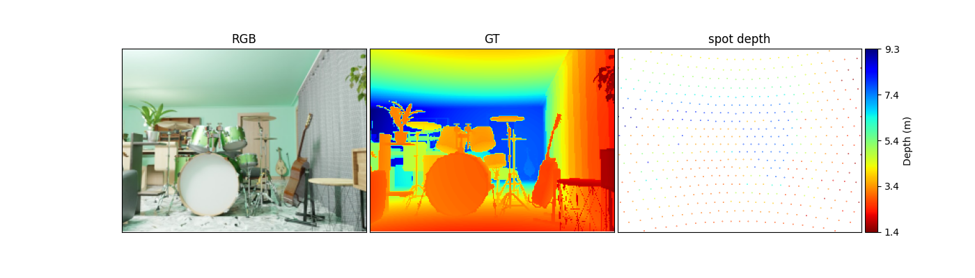
Figure 1: Visualization of an example training data. Left, middle, and right images correspond to RGB, ground-truth depth, and simulated spot depth data, respectively.

The testing data contains, a) Synthetic: a synthetic image sequence (500 pairs of RGB and depth in total) rendered from an indoor virtual environment that differs from the training data; b) iPhone dynamic: 24 image sequences of dynamic scenes collected from an iPhone 12Pro (600 pairs of RGB and depth in total); c) iPhone static: 24 image sequences of static scenes collected from an iPhone 12Pro (600 pairs of RGB and depth in total); d) Modified phone static: 24 image sequences of static scenes (600 pairs of RGB and depth in total) collected from a modified phone. Please note that depth noises, missing depth values in low reflectance regions, and mismatch of the field of views between RGB and ToF cameras could be observed from this real data. RGB and dense depth images in the entire testing set have a resolution of 256$\times$192 pixels. RGB and spot depth data from the testing set are provided and the GT depth is not available to participants. The depth data in both training and testing sets are in meters.

2.3 Challenge Phases

The challenge consisted of the following phases:

1. Development: The registered participants get access to the data and baseline code, and are able to train the models and evaluate their running time locally.

2. Validation: The participants can upload their models to the remote server to check the fidelity scores on the validation dataset, and to compare their results on the validation leaderboard.

3. Testing: The participants submit their final results, code, models, and factsheets.

2.4 Performance Evaluation

2.4.1 Objective Evaluation

We define the following metrics to evaluate the performance of depth completion algorithms.

• Relative Mean Absolute Error (RMAE), which measures the relative depth error between the completed depth and the ground truth, i.e.

  $$\small\text{RMAE}=\frac{1}{M\cdot N}\sum_{m=1}^{M}\sum_{n=1}^{N}\left\lvert\frac{\hat{D}(m,n)-D(m,n)}{D(m,n)}\right\rvert,$$ (1)

  where $M$ and $N$ denote the height and width of depth, respectively. $D$ and $\hat{D}$ represent the ground-truth depth and the predicted depth, respectively.

• Edge Weighted Mean Absolute Error (EWMAE), which is a weighted average of absolute error. Regions with larger depth discontinuity are assigned higher weights. Similar to the idea of Gradient Conduction Mean Square Error (GCMSE) [17], EWMAE applies a weighting coefficient $G(m,n)$ to the absolute error between pixel $(m,n)$ in ground-truth depth $D$ and predicted depth $\hat{D}$, i.e.

  $$\begin{array}[]{l}\text{EWMAE}=\\ \frac{1}{M\cdot N}\left\lvert\frac{\sum\limits_{m=1}^{M}\sum\limits_{n=1}^{N}G(m,n)\cdot[\hat{D}(m,n)-D(m,n)]}{\sum\limits_{m=1}^{M}\sum\limits_{n=1}^{N}G(m,n)}\right\rvert\end{array},$$ (2)

  where the weight coefficient $G$ is computed in the same way as in [17].

RMAE and EWMAE will be measured on the testing data with GT depth. We will rank the proposed algorithms according to the score calculated by the following formula, where the coefficients are designed to balance the values of different metrics,

$$\text{Objective score}=1-1.8\times\text{RMAE}-0.6\times\text{EWMAE}.$$ (3)

For each dataset, we report the average results over all the processed images belonging to it.

2.4.2 Subjective Evaluation

For subjective evaluation, we adapt the commonly used Mean Opinion Score (MOS) with blind evaluation. The score is on a scale of 1 (bad) to 5 (excellent). We invited 13 expert observers to watch videos and give their subjective scores independently. The scores of all subjects are averaged as the final MOS.

2.5 Running Time Evaluation

The proposed algorithms are required to be able to process the RGB and sparse depth sequence in real time. Participants are required to include the average run time of one pair of RGB and depth data using their algorithms and the information in the device in the submitted readme file. Due to the difference of devices for evaluation, we set different requirements of running time for different types of devices according to the AI benchmark data from the website.

3 Challenge Results

Table 1: MIPI 2023 RGB+ToF Depth Completion challenge results and final rankings.

Rank	Team name	RMAE	EWMAE	Objective score	Subjective score	Final score
1	MGTV	0.02164	0.13257	0.88151	3.60577	0.80133
2	MiMcAlgo	0.01921	0.13462	0.88465	3.38846	0.78117
3	Dintel	0.02702	0.13569	0.86995	3.06731	0.74171
4	Chameleon	0.02232	0.13305	0.87999	2.90385	0.73038

Among $77$ registered participants, $4$ teams successfully submitted their results, code, and factsheets in the final test phase. Table 1 summarizes the final test results and rankings of the teams. Team MGTV shows the best overall performance, followed by Team MiMcAlgo and Team DIntel. The proposed solutions are described in Section 4 and the team members and affiliations are listed in Appendix A.

4 Challenge Methods

4.1 MGTV

Model.This team has proposed a model architecture, as illustrated in Figure 2, that incorporates ResNet34 [7] for the Encoder module, while the Decoder module is composed of a sequence of 5 upsample blocks, each of which integrates a convolutional layer, a pixel shuffle layer, and a channel attention branch [10]. The Local Network is a concatenation of three consecutive convolutional layers, while the Refined Network capitalizes on the FCSPNet [8] for optimal performance.

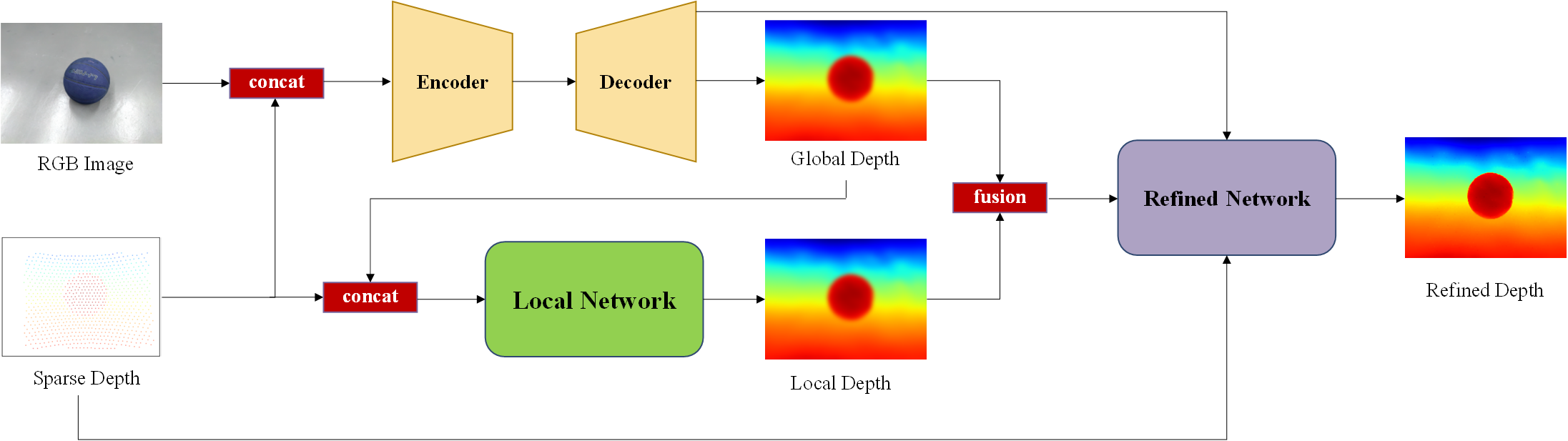
Figure 2: Framework of the MGTV team

Loss.This team employed three loss functions jointly for training, namely L1 loss, RMAE loss, and Gradient loss proposed by  [8]. In the early stage, in order to ensure the stability of model training, the L1 losses were calculated for global depth, local depth, and refined depth simultaneously. After the model training became stable, only the L1 loss for refined depth was calculated to obtain optimal results.

Data augmentation.This team observed that the sparse depth inputs in the testing data were not all sampled on a regular grid. During training, This team randomly applied local and circular removal operations to the sparse depth inputs with a certain probability, to simulate the input distribution of sparse depth data in the testing phase. This approach not only enhanced the generalization capability of the model but also improved its performance on such testing data.

Outlier handling. This team observed that the sparse depth inputs in the testing data have some outliers which will introduce bias in the predictions around them. So this team removed the outliers beyond 3 standard deviations from the mean during the inference phase.

4.2 MiMcAlgo

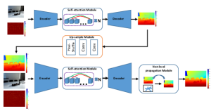
Figure 3: Overview of EMNLP-TN.

Method. The team has developed an effective and efficient method for depth completion called Enhancing Multi-Scale Non-Local Propagation with Transformer Network (EMNLP-TN), illustrated in Figure 3.
Coarse-to-fine prediction: The proposed method, EMNLP-TN, employs a two-stage approach for depth completion, which shares similarities with the method outlined in penet [11]. However, EMNLP-TN utilizes a coarse-to-fine framework that addresses the complexity of depth completion in two sub-problems: structure prediction and detail refinement. In both stages, the same encoder and decoder network are utilized. Specifically, the second stage takes the coarse depth prediction from the first stage as input and applies several non-local spatial propagation networks [19] to enhance the prediction.
Artifacts-free up-sample: From the perspective of super-resolution, completion can also be seen as the process of interpolating missing depth information using RGB image guidance. This makes depth completion an equivalent process to depth super-resolution. To achieve this, the team used the pixel-shuffle[1] operation from super-resolution to bridge the gap between downscaled and full-sized depth data.

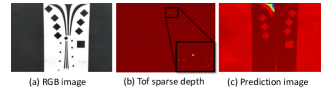
Figure 4: Bad point result.

Self-attention: Depth completion is distinct from stereo depth because it does not rely on depth cues from the input. Instead, it leverages sparse depth information to label segments or pixels and learns semantic and segmentation information from RGB images. As demonstrated by the example illustrated in Figure 4, the flat input image can yield widely varying depths in different segments due to shortcomings in the sparse depth map. The results confirm that the network learns more segmentation information rather than depth. This indicates that the network is learning more about segmentation than depth. To address this issue, the team employed a transformer[23] to extract global features for better segmentation. The self-attention module of light LoFTR[21] is introduced to aggregate more sparse depth points.

Training loss. Each branch is trained with

$$Loss=\alpha*RMAE+\beta*EWMAE.$$ (4)

Specifically, the loss shares the same formulation as RMAE and EWMAE metrics.
The total loss of EMNLP-TN can be described as follow

$$Loss_{total}=Loss_{corase}+Loss_{fine}.$$ (5)

4.3 DIntel

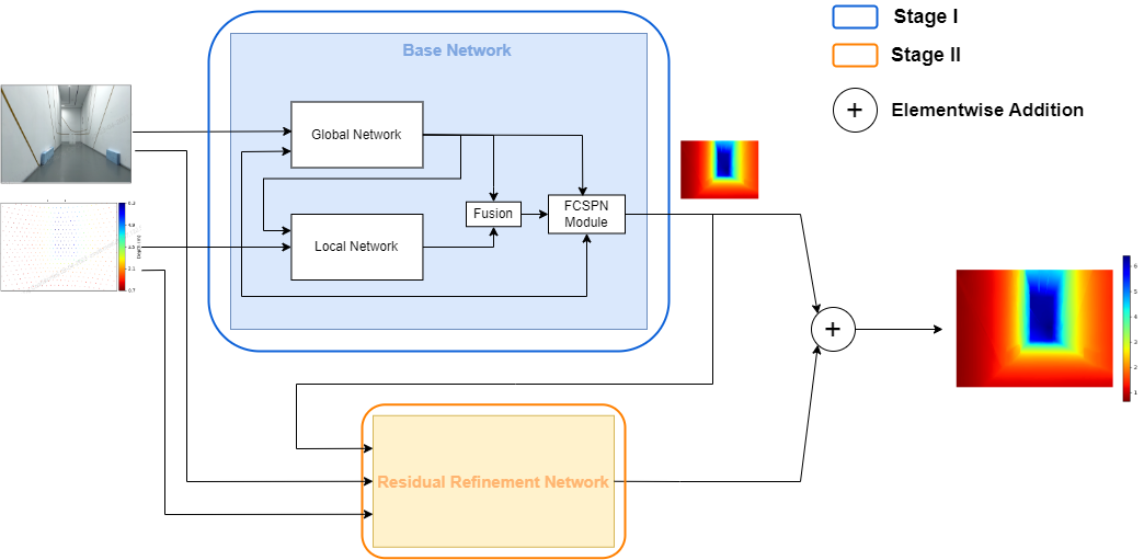
Figure 5: Overview of DIntel architecture

Model. This team uses a cascaded residual refinement approach for the depth completion task. In this cascaded style network architecture, the authors have used two network modules: Base Network and Residual Refinement Network (RRN), as shown in Figure 5. Inspired from [8], the base network’s architecture gives local and global depth predictions, which are then fused and passed through a few more layers to get the affinity matrix for funnel convolutional spatial propagation network (FCSPN) module, which in turn gives the initial refined depth map prediction. The output of the base network, along with RGB image and spot depth, is then fed as input to the RRN (a ResNet-34 [7] based architecture), whose objective is to rectify the incorrect depth predictions from the base network.

Training. The base network was trained similarly to [8]. After training the base network, the weights of the base network were frozen, and only the RRN was trained. RRN was trained for 42 epochs with a batch size of 16. The initial learning rate was 0.001 with a decay factor of {1.0, 0.2, 0.04} at epochs {10, 15, 20}. To tackle the missing sparse depth challenge in the test dataset, the authors trained the model by removing the spot depth from random areas of the image.

Loss. In the base network and RRN, the authors have used a combination of $L_{1}$, $L_{2}$ and Corrected Gradient Loss (CGDL) [8] with adaptive weights of 1, 1 and 0.7, respectively. While $L_{1}$ and $L_{2}$ losses helped get accurate depths, the main objective of CGDL loss was to keep the depth prediction output smooth and edges sharp.

4.4 Chameleon

Model. This team propose an effective and efficient depth completion method for depth completion called Bilateraly-Aware Depth Completion via Cascaded Dynamic Grapth Convolutional Network (CDGNN-BA), illustrated in Figure 6. The proposed method, CDGNN-BA, outputs dense depth and follows the Convolutional Spatial Propagation Network, originally introduced in [4]. In particular, this team start out with Dynamic Grapth Convolutional Network design as in GraphCSPN [16] and propose modifications for further improvement as below.

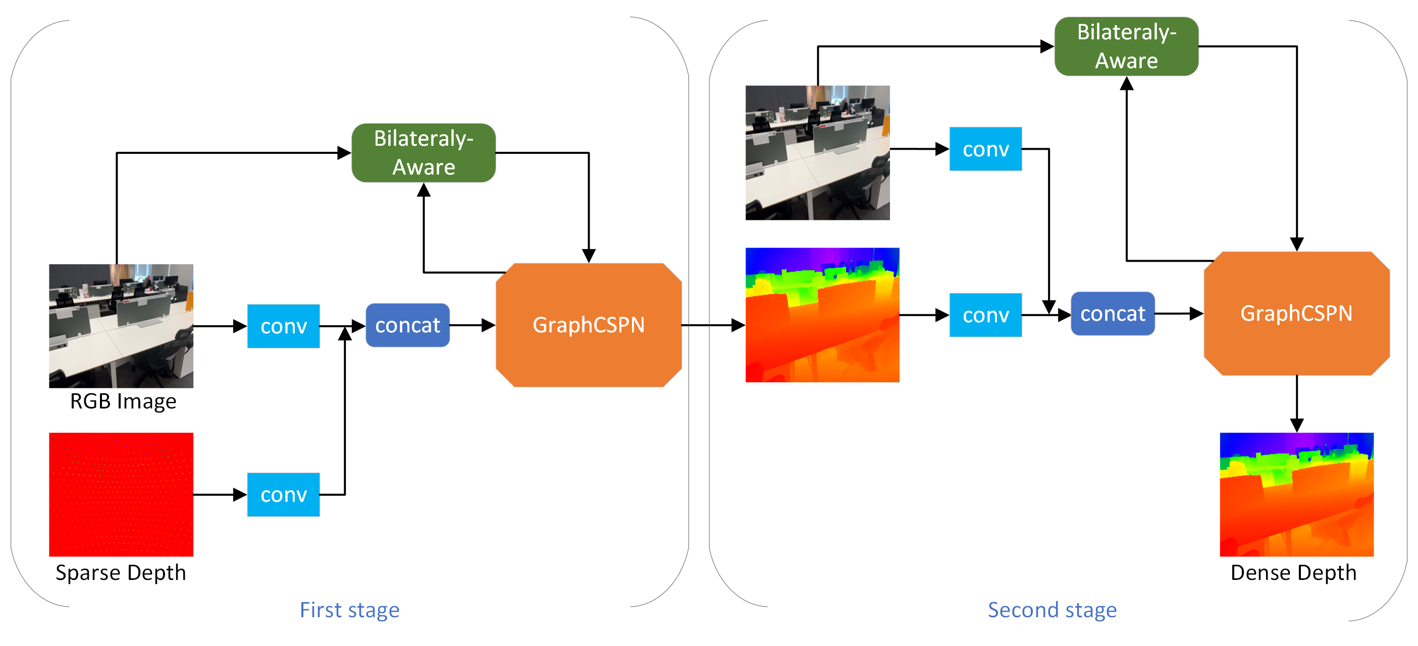
Figure 6: Pipeline of CDGNN-BA.

Bilateraly-Aware: GraphCSPN utilizes an encoder-decoder to jointly learn the initial depth map and affinity matrix, which is sampled and reshaped into sequences of patches and concatenated with 3D position embeddings. Then the model estimates the neighbors of different patches on the basis of geometric constraints, and performs spatial propagation leveraging dynamic graph convolution networks with self-attention mechanism. After the graph is generated, the Top k patches are judged, and the weighted sum is obtained to predict the final depth. However, the way of calculating the similarity only considers the physical distance between patches while the heterochromia from various objects is ignored. In our method, the RGB information is considered based on the fact that patches from the same object have a higher correlation; Additionally, the naive 3D reconstruction requires camera internal parameters which are hard to obtain in several scenarios. Instead of using these parameters, the authors utilized the distances between pixels and depth distance from the depth map. In particular, the above distance weights are calculated using bilateral weight:

$$d=e^{(-\frac{(d_{rgb}-u_{rgb})^{2}}{2\sigma_{rgb}^{2}}-\frac{(d_{pixel}-u_{pixel})^{2}}{2\sigma_{pixel}^{2}}-\frac{(d_{depth}-u_{depth})^{2}}{2\sigma_{depth}^{2}})}.$$ (6)

Cascaded refinement: GraphCSPN re-samples the affinity matrix by 3-time losses the information of original features. For compensating this deficiency, the cascade structure is proposed. First, 4-time down-sampling is performed. After graph propagation, coarse depth is obtained, and then 2-time down-sampling is applied to obtain refined depth.

Loss. This team uses the same loss function as Equation 4

Training Setup. For training, this team randomly cropped and resized 192 × 256 patches from the training images as inputs. The mini-batch size is set to 4 and the whole network is trained for 200 epochs. The learning rate is initialized as $1\times 10^{-3}$, decayed with a LinearLR schedule.

5 Conclusions

In this report, we review and summarize the methods and results of MIPI 2023 challenge on RGB+ToF Depth Completion. The participants were provided with a high-quality training/testing dataset, TetrasRGBD, which is now available for researchers to download for future research. We are excited to see the new progress contributed by the submitted solutions in such a short time, which are all described in this paper. The challenge results are reported and analyzed. Detailed descriptions of the submitted solutions are also provided in this report. For future works, there is still plenty of room for improvements including dealing with depth outliers/noises, precise depth boundaries, high depth resolution, and high temporal stability, etc.

6 Acknowledgements

We thank Shanghai Artificial Intelligence Laboratory, Sony, Nanyang Technological University and The Chinese University of Hong Kong to sponsor this MIPI 2023 challenge. We thank all the organizers for their contributions to this workshop and all the participants for their great work.

Appendix A Teams and Affiliations

MGTV team

Title: MangoTV
Members:
YiYu¹ (yuyi@mgtv.com)
YangkeHuang¹(yangke5@mgtv.com) KangZhang¹(zhangkang@mgtv.com)
Affiliations:
¹ MGTV (https://w.mgtv.com/)

MiMcAlgo team

Title: Enhancing Multi-Scale Non-Local Propagation with Transformer Network.

Members:
Meiya Chen (chenmeiya@xiaomi.com)
Yu Wang (wangyu50@xiaomi.com)
Yongchao Li (liyongchao1@xiaomi.com)
Hao Jiang (jianghao11@xiaomi.com)

Affiliations:
Xiaomi Inc.

DIntel team

Title: Efficient and Refined Multi-modal Depth Completion
Members:
Amrit Kumar Muduli (amrit.muduli@samsung.com)
Vikash Kumar (vikash.k7@samsung.com)
Kunal Swami (kunal.swami@samsung.com)
Pankaj Kumar Bajpai (pankaj.b@samsung.com)
Affiliation:
Samsung R & D Institute India - Bangalore

Chameleon team

Title: Bilateraly-Aware Depth Completion via Cascaded Dynamic Grapth Convolutional Network

Members:
Yunchao Ma (mayunchao@megvii.com)
Jiaojun Xiao (xiaojiajun@megvii.com)
Zhi Ling (lingzhi@megvii.com)

References

- [1] Andrew Aitken, Christian Ledig, Lucas Theis, Jose Caballero, Zehan Wang, and Wenzhe Shi. Checkerboard artifact free sub-pixel convolution: A note on sub-pixel convolution, resize convolution and convolution resize. arXiv preprint arXiv:1707.02937, 2017.
- [2] Zhao Chen, Vijay Badrinarayanan, Gilad Drozdov, and Andrew Rabinovich. Estimating depth from rgb and sparse sensing. In Proceedings of the European Conference on Computer Vision (ECCV), pages 167–182, 2018.
- [3] Xinjing Cheng, Peng Wang, Chenye Guan, and Ruigang Yang. Cspn++: Learning context and resource aware convolutional spatial propagation networks for depth completion. In Proceedings of the AAAI Conference on Artificial Intelligence, volume 34, pages 10615–10622, 2020.
- [4] Xinjing Cheng, Peng Wang, and Ruigang Yang. Learning depth with convolutional spatial propagation network. IEEE transactions on pattern analysis and machine intelligence, 42(10):2361–2379, 2019.
- [5] Abdelrahman Eldesokey, Michael Felsberg, Karl Holmquist, and Michael Persson. Uncertainty-aware cnns for depth completion: Uncertainty from beginning to end. In Proceedings of the IEEE/CVF Conference on Computer Vision and Pattern Recognition, pages 12014–12023, 2020.
- [6] Abdelrahman Eldesokey, Michael Felsberg, and Fahad Shahbaz Khan. Confidence propagation through cnns for guided sparse depth regression. IEEE Transactions on Pattern Analysis and Machine Intelligence, 42(10):2423–2436, 2019.
- [7] Kaiming He, Xiangyu Zhang, Shaoqing Ren, and Jian Sun. Deep residual learning for image recognition. In Proceedings of the IEEE conference on computer vision and pattern recognition, pages 770–778, 2016.
- [8] Dewang Hou, Yuanyuan Du, Kai Zhao, and Yang Zhao. Learning an efficient multimodal depth completion model. In Computer Vision–ECCV 2022 Workshops: Tel Aviv, Israel, October 23–27, 2022, Proceedings, Part V, pages 161–174. Springer, 2023.
- [9] Junjie Hu, Chenyu Bao, Mete Ozay, Chenyou Fan, Qing Gao, Honghai Liu, and Tin Lun Lam. Deep depth completion: A survey. arXiv preprint arXiv:2205.05335, 2022.
- [10] Jie Hu, Li Shen, and Gang Sun. Squeeze-and-excitation networks. In Proceedings of the IEEE conference on computer vision and pattern recognition, pages 7132–7141, 2018.
- [11] Mu Hu, Shuling Wang, Bin Li, Shiyu Ning, Li Fan, and Xiaojin Gong. Penet: Towards precise and efficient image guided depth completion. In 2021 IEEE International Conference on Robotics and Automation (ICRA), pages 13656–13662. IEEE, 2021.
- [12] Saif Imran, Yunfei Long, Xiaoming Liu, and Daniel Morris. Depth coefficients for depth completion. In Proceedings of the IEEE/CVF Conference on Computer Vision and Pattern Recognition, pages 12438–12447. IEEE, 2019.
- [13] Byeong-Uk Lee, Kyunghyun Lee, and In So Kweon. Depth completion using plane-residual representation. In Proceedings of the IEEE/CVF Conference on Computer Vision and Pattern Recognition, pages 13916–13925, 2021.
- [14] Ang Li, Zejian Yuan, Yonggen Ling, Wanchao Chi, Chong Zhang, et al. A multi-scale guided cascade hourglass network for depth completion. In Proceedings of the IEEE/CVF Winter Conference on Applications of Computer Vision, pages 32–40, 2020.
- [15] Yuankai Lin, Tao Cheng, Qi Zhong, Wending Zhou, and Hua Yang. Dynamic spatial propagation network for depth completion. arXiv preprint arXiv:2202.09769, 2022.
- [16] Xin Liu, Xiaofei Shao, Bo Wang, Yali Li, and Shengjin Wang. Graphcspn: Geometry-aware depth completion via dynamic gcns. In Computer Vision–ECCV 2022: 17th European Conference, Tel Aviv, Israel, October 23–27, 2022, Proceedings, Part XXXIII, pages 90–107. Springer, 2022.
- [17] Javier López-Randulfe, César Veiga, Juan J Rodríguez-Andina, and José Farina. A quantitative method for selecting denoising filters, based on a new edge-sensitive metric. In 2017 IEEE International Conference on Industrial Technology (ICIT), pages 974–979. IEEE, 2017.
- [18] Adrian Lopez-Rodriguez, Benjamin Busam, and Krystian Mikolajczyk. Project to adapt: Domain adaptation for depth completion from noisy and sparse sensor data. In Proceedings of the Asian Conference on Computer Vision, 2020.
- [19] Jinsun Park, Kyungdon Joo, Zhe Hu, Chi-Kuei Liu, and In So Kweon. Non-local spatial propagation network for depth completion. In In: Proceedings of the European Conference on Computer Vision (ECCV), pages 120–136. Springer, 2020.
- [20] Chao Qu, Ty Nguyen, and Camillo Taylor. Depth completion via deep basis fitting. In Proceedings of the IEEE/CVF Winter Conference on Applications of Computer Vision, pages 71–80, 2020.
- [21] Jiaming Sun, Zehong Shen, Yuang Wang, Hujun Bao, and Xiaowei Zhou. Loftr: Detector-free local feature matching with transformers. In In: Proceedings of the IEEE/CVF Conference on Computer Vision and Pattern Recognition (CVPR), pages 8922–8931, 2021.
- [22] Wenxiu Sun, Qingpeng Zhu, Chongyi Li, Ruicheng Feng, Shangchen Zhou, Jun Jiang, Qingyu Yang, Chen Change Loy, Jinwei Gu, Dewang Hou, et al. Mipi 2022 challenge on rgb+ tof depth completion: Dataset and report. In Computer Vision–ECCV 2022 Workshops: Tel Aviv, Israel, October 23–27, 2022, Proceedings, Part V, pages 3–20. Springer, 2022.
- [23] Ashish Vaswani, Noam Shazeer, Niki Parmar, Jakob Uszkoreit, Llion Jones, Aidan N Gomez, Łukasz Kaiser, and Illia Polosukhin. Attention is all you need. Advances in neural information processing systems, 30, 2017.