Massive Dark Matter Halos at High Redshift: Implications for Observations in the JWST Era

Abstract

The presence of massive galaxies at high $z$ as recently observed by JWST appears to contradict the current $\Lambda$CDM cosmology. Here we aim to alleviate this tension by incorporating uncertainties from three sources in counting galaxies: cosmic variance, error in stellar mass estimation, and backsplash enhancement. Each of these factors significantly increases the cumulative stellar mass density $\rho_{*}(>M_{*})$ at the high-mass end, and their combined effect can boost the density by more than one order of magnitude. Assuming a star formation efficiency of $\epsilon_{*}\sim 0.5$, cosmic variance alone reduces the tension to a $2\sigma$ level, except for the most massive galaxy at $z=8$. Additionally, incorporating a 0.3 dex lognormal dispersion in the stellar mass estimation brings the observed $\rho_{*}(>M_{*})$ at $z\sim 7-10$ within $2\sigma$. The tension is completely eliminated when we account for the gas stripped from backsplash halos. These results highlight the importance of fully modeling uncertainties when interpreting observational data of rare objects. We use the constrained simulation, ELUCID, to investigate the descendants of high-$z$ massive galaxies. Our findings reveal that a significant portion of these galaxies ultimately reside in massive halos at $z=0$ with $M_{\rm halo}>10^{13}\,h^{-1}{\rm M_{\odot}}$. Moreover, a large fraction of local central galaxies in $M_{\rm halo}\geqslant 10^{14.5}\,h^{-1}{\rm M_{\odot}}$ halos are predicted to contain substantial amounts of ancient stars formed in massive galaxies at $z\sim 8$. This prediction can be tested by studying the structure and stellar population of central galaxies in present-day massive clusters.

1 Introduction

The launch of the James Webb Space Telescope (JWST) in late 2021 opens a new era in the study of galaxy formation and evolution. As an upgrade to its predecessor, Hubble Space Telescope (HST), the $\sim 7\times$ light-gathering power, longer wavelength coverage, higher sensitivity of infrared imaging and spectroscopy equip JWST with unprecedented capability for detecting galaxies at high-redshift. Recent analyses based on Cycle 1 early data releases from early release observations (ERO) programs, such as ERO SMACS J0723 and Stephans’s Quintet, as well as on early release science (ERS) programs, such as Cosmic Evolution Early Release Science (CEERS, Finkelstein et al., 2017, 2022, 2023) and GLASS James Webb Space Telescope Early Release Science (GLASS, Treu et al., 2017), have revealed dozens of luminous galaxies at redshift ranging from $z\sim 7$ to $\sim 20$ (Naidu et al., 2022; Rodighiero et al., 2022; Donnan et al., 2022; Finkelstein et al., 2022; Bouwens et al., 2023; Finkelstein et al., 2023; Harikane et al., 2023; Labbé et al., 2023). Theoretical followups have suggested that the high UV luminosity and stellar mass of the observed candidates are inconsistent with nearly all existing galaxy formation models, including those built with empirical methods, semianalytical methods, and hydrodynamic simulations (Mason et al., 2023; Naidu et al., 2022; Rodighiero et al., 2022; Harikane et al., 2023; Labbé et al., 2023; Finkelstein et al., 2023). This discrepancy is even in significant tension with the upper limit permitted by the current LambdaCDM model (Lovell et al., 2022; Boylan-Kolchin, 2023). However, given the uncertainties in both galaxy formation models and observational measurements, it may be premature to draw any definitive conclusions.

Various arguments have been put forward to address these tensions from different perspectives. For instance, Mason et al. (2023) employed empirical methods to derive upper limits on the UV luminosity functions at redshifts of $z\sim 8-20$, and found that the JWST observations are well within these limits. A comprehensive study by Harikane et al. (2023) suggested that the lack of reionization sources at $z\gtrsim 10$ to suppress star formation, or a top-heavy initial mass function (IMF) expected for Pop-III stars in a lower-metallicity environment exposed to higher cosmic microwave background (CMB) temperature, could increase the UV luminosity by a factor of $\lesssim 4$, thus marginally resolving the $1\,{\rm dex}$ difference between model and observation. Yung et al. (2023) arrived at similar conclusions that a modest boost of a factor of $\sim 4$ to the UV luminosities, possibly due to a top-heavy IMF, can resolve the $\gtrsim 1\,{\rm dex}$ discrepancy between the Santa-Cruz semi-analytical model (SAM) and observations at $z\gtrsim 10$. They also suggested another modification to the star formation model, assuming a lower stellar feedback strength, to address the tension. Kannan et al. (2023) proposed that new processes should be incorporated into hydrodynamic simulations to match the observed star formation rate density.

Recent observational results by Labbé et al. (2023) at redshifts of $z\sim 7-10$ present even more tensions with current hierarchical galaxy formation models under the $\Lambda$CDM cosmology. Using double-break selected galaxies from the JWST CEERS sample, they identified six candidate galaxies with stellar masses $M_{*}\geq 10^{10}\,h^{-1}{\rm M_{\odot}}$, with one extreme galaxy having a mass of nearly $10^{11}\,h^{-1}{\rm M_{\odot}}$. To derive redshift and stellar mass, they used the photometry in 10 bands from JWST/NIRCam + HST/ACS observations, as well as seven different SED fitting code settings (EAZY, Prospector, and five Bagpipes settings). Compared to earlier results from HST+Spitzer measurements (Stefanon et al., 2021), the cosmic stellar mass density reported by Labbé et al. (2023) is a factor of $\sim 20$ higher at $z\sim 8$ and a factor of $\sim 1000$ higher at $z\sim 9$. If these findings are confirmed by future spectroscopic surveys, such as those conducted with JWST/NIRSpec, they present a serious challenge to the standard $\Lambda$CDM paradigm, because the observed stellar masses exceed the upper limit allowed by the cosmic baryon fraction.

Several theoretical follow-ups have been conducted to explain the observational result by Labbé et al. (2023). Using theoretical halo mass functions from the Press-Schechter formalism given by Sheth & Tormen (1999) and assuming a maximal star formation efficiency, Boylan-Kolchin (2023) showed that the two most massive candidates identified by Labbé et al. (2023) represent a $\sim 3\sigma$ tension. Even taking into account uncertainties in stellar mass, sampling and Poisson fluctuation, their results still require that the star formation efficiency at $z=9$ be $\epsilon_{*}(z=9)\geqslant 0.57$. The tension would be even more severe given that the Sheth-Tormen halo mass functions are $20\%-50\%$ higher than those obtained from N-body simulations in the same redshift range. Lovell et al. (2022) performed more stringent tests using halo mass functions from N-body simulations and Extreme Value Statistics (EVS), and revealed a tension at $>3\sigma$ level between the sample of Labbé et al. (2023) and the expectation from the extreme assumption of $\epsilon_{*}=1$. Although the results may change with updated calibration in the photometry of JWST/NIRCam, the qualitative conclusion is expected to remain.

There are several issues with summary statistics obtained from galaxies of extreme masses. Firstly, uncertainties in the stellar mass estimate can be amplified by the steepness of the stellar mass function at the high-mass end, and can lead both to larger scatter and bias towards higher values - a phenomenon known as Eddington bias (Eddington, 1913). Secondly, as errors from different sources may interact non-linearly, incomplete modeling of the sources of uncertainties can potentially change the statistical result significantly. Finally, the highly skewed and discrete error distribution makes it difficult to represent accurately the error distribution with centralized and symmetric analytical approximations. All these issues have important implications for interpreting observational results in terms of theoretical expectations.

In observations, a summary statistic, $s$, is usually represented and plotted as $(s_{0}-\Delta s_{\rm lower},s_{0}+\Delta s_{\rm upper})$, where $s_{0}$ is interpreted as an estimate of the mean or median of the underlying random variable $s$, and $\Delta s_{\rm lower}$ and $\Delta s_{\rm upper}$ represent the standard deviation or quantile. However, with biased observations and asymmetric error distributions, the $s_{0}\pm\Delta$ error representation deviates from its commonly-assumed physical meaning and may mislead observation-theory comparisons. A solution to these issues is the forward approach supported by Bayesian theory. Lovell et al. (2022) provided an example by using extreme values of stellar mass, instead of direct counting, and forward modeling of errors based on halo mass functions and volume sampling to bypass the issues described above. However, the volume sampling technique, error modeling, and correction for Eddington bias are likely too simplified in their implementation. Meanwhile, summary statistics, such as galaxy number density and cosmic stellar mass/SFR density, are important scientific products of many HST/Spitzer/JWST observations and serve as the entry point for observation-theory comparisons.

In this study, we propose a forward modeling approach of galaxy counting and demonstrate the impact of different sources of uncertainties on observational results. We begin with an N-body simulation, populate halos with galaxies through consecutive transformations, and incorporate various sources of uncertainties in these steps. We carefully devise both the representation of errors and the method for comparison with high-redshift data. Using a constrained simulation that reconstructs the assembly history of real clusters of galaxies at $z\sim 0$, we provide insights into the low-$z$ descendants of the observed high-redshift galaxies.

The paper is organized as follows. In §2, we describe the N-body simulation we use, the method to populate halos with galaxies, and the approach to incorporating uncertainties. In §3, we highlight the impact of these uncertainties on the interpretation of recent JWST observations at $z\sim 7-10$. We will show that the tension with the standard $\Lambda$CDM can be reduced significantly or even completely eliminated by taking these uncertainties properly into account. In §4, we present the descendant properties of high-redshift massive galaxies and discuss their implications for observations.

2 Data and Analysis

2.1 The ELUCID Simulation

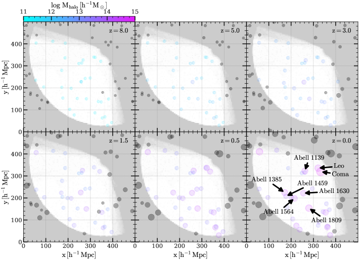
Figure 1: Massive halos selected at $z=8$ with $M_{\rm halo}\geqslant 2\times 10^{11}\,h^{-1}{\rm M_{\odot}}$ from a spatial slice with $50\,h^{-1}{\rm{Mpc}}$ thickness in the constrained simulation of ELUCID (top-left panel) and their descendant halos at lower redshifts (other panels). Descendant halos at $z=0$ in the simulation are matched with observed clusters in the local Universe, as indicated in the lower-right panel with names or Abell indices. The gray shaded area in each panel marks the out-of-reconstruction volume, while the unmasked area is the volume whose density field is constrained by galaxy groups from SDSS. Out-of-reconstruction halos are represented by gray circles. In-reconstruction halos are represented by colored circles, whose sizes and colors are scaled according to their masses. For a detailed description of the constrained simulation and halo sample, refer to §2. For a discussion about the evolution of halos, see §4.

Throughout this paper, we use ELUCID (Wang et al., 2016), a constrained N-body simulation obtained using the code L-Gadget, a memory-optimized version of Gadget-2 (Springel, 2005). The simulation uses a WMAP5 (Dunkley et al., 2009) cosmology with the following parameters: $\Omega_{\rm K,0}=0$, $\Omega_{\rm M,0}=0.258$, $\Omega_{\rm B,0}=0.044$, $\Omega_{\rm\Lambda,0}=0.742$, $H_{0}=100\ h\,{\rm km\,s^{-1}\,Mpc^{-1}}$ with $h=0.72$, and a spectral index of $n=0.96$ with an amplitude specified by $\sigma_{8}=0.80$ for the Gaussian initial density field. A total of 100 snapshots, from redshift $z=18.4$ to $0$, are saved. Halos are identified using the friends-of-friends (FoF) algorithm (Davis et al., 1985) with a scaled linking length of $0.2$. Subhalos are identified using the Subfind algorithm (Springel et al., 2001; Dolag et al., 2009), and subhalo merger trees are constructed using the SubLink algorithm (Springel, 2005; Boylan-Kolchin et al., 2009). ELUCID has a simulation box with a side length of $500\,h^{-1}{\rm{Mpc}}$ and uses a total of $3072^{3}$ particles to trace the cosmic density field. The mass of each dark matter particle is $3.08\times 10^{8}\,h^{-1}{\rm M_{\odot}}$, and the mass resolution limit of FoF halos is about $10^{10}\,h^{-1}{\rm M_{\odot}}$. As we only use halos well above this limit to model massive galaxies, the relatively low resolution of ELUCID does not affect our conclusions. Additionally, because all the uncertainties considered here are significant, the slight difference in cosmological parameters between WMAP5 and the more recent Planck data does not have a significant impact on our findings.

The initial condition of ELUCID is reconstructed from real galaxy groups identified from the SDSS (Yang et al., 2007; Yang et al., 2012) by a sequence of numerical methods detailed in Wang et al. (2016). Analysis based on cross-matching the simulated and observed halos at $z\sim 0$ showed that more than $95\%$ of massive halos with halo mass $M_{\rm halo}\geqslant 10^{14}\,h^{-1}{\rm M_{\odot}}$ can be recovered in the constrained simulation with a $0.5\,{\rm dex}$ tolerance on the error of halo mass and a $4\,h^{-1}{\rm{Mpc}}$ tolerance on the error of spatial location. These features of ELUCID enable not only the statistical study of halo and galaxy populations within it, but also a halo-by-halo comparison to massive clusters in the real universe. In §3, we use ELUCID to statistically infer uncertainties in measuring the abundance of extremely massive galaxies at $z=7\sim 10$, and in §4, we use ELUCID to study the assembly history of several real massive clusters in the local universe. The bottom-right panel of Fig. 1 shows some examples of the matched clusters in a slice of the simulation volume, including two massive clusters, Coma and Leo, and a number of Abell clusters (Abell et al., 1989; Struble & Rood, 1999).

2.2 Method to Evaluate Uncertainties in Galaxy Counting

Here we take ELUCID as the input, populate dark matter halos with galaxies and estimate the uncertainties in counting galaxies for surveys at high $z$. Our goal is to estimate the uncertainty of a given summary statistic, $s_{*}$, of galaxies in a sub-volume whose geometry is consistent with the survey in question, starting from the sample $S_{\rm halo}$ of all halos at a given redshift $z$ in ELUCID. To achieve this, we decompose the transformation from $S_{\rm halo}$ to $s_{*}$ into a chain of four steps based on our understanding of galaxy formation in the $\Lambda$CDM paradigm:

$$s_{*}=\mathcal{T}_{\rm stat}\circ\mathcal{T}_{M_{*}}\circ\mathcal{T}_{M_{\rm halo}}\circ\mathcal{T}_{\rm CV}(S_{\rm halo})\,,$$ (1)

where $\mathcal{T}_{\rm CV}$ denotes the volume-based sub-sampling of halos, $\mathcal{T}_{M_{\rm halo}}$ denotes the determination of the mass $M_{\rm halo}$ for each halo in the sub-sample, $\mathcal{T}_{M_{*}}$ denotes the halo-to-galaxy mapping, and $\mathcal{T}_{\rm stat}$ denotes the statistical function that extracts the summary statistic from the galaxy sample. We will describe numerical implementations of these steps in detail later.

As discussed in §1, there are multiple uncertainties that are critical in estimating $s_{*}$. Our decomposition strategy described above ensures that each type of uncertainty can be physically modeled in the relevant step, and that the forward incorporation of all steps naturally propagates all uncertainties into the total uncertainty of $s_{*}$. In addition, this also allows us to quantify contributions of individual uncertainties by incrementally adding them into the chain.

In principle, the counts of halos are noisy because massive objects are rare in a small volume by definition. This sampling uncertainty is further enhanced by other sources of uncertainty in the halo-to-galaxy mapping due to the increased steepness of the Schechter function toward the high-mass end. Additionally, as the sample size goes below $\sim 100$, the discreteness in galaxy counts and its skewness must be carefully taken into account (e.g., Trenti & Stiavelli, 2008). To address these issues, we deliberately choose the cumulative cosmic stellar mass density, $s_{*}=\rho_{*}(>M_{*})$, as the summary statistic when comparing the theoretical prediction with observational data (see also Labbé et al., 2023; Lovell et al., 2022; Boylan-Kolchin, 2023, for the same usage). We describe the uncertainty of $s_{*}$ using the probability distribution, $P(s_{*})$, instead of summary statistics with compressed information, such as the average, variance, and quantile. If desired, these compressed quantities can be estimated from $P(s_{*})$.

In the following, we specify each of the transformations involved in the mapping from halos to galaxy statistic and describe uncertainties injected into them.

Volume sampling operator: The transformation $\mathcal{T}_{\rm CV}$, implemented by drawing a sub-volume from the periodic box of ELUCID and filtering out all halos from $S_{\rm halo}$ outside the selected volume, constitutes the volume sampling operator. The uncertainty in the sampling is naturally incorporated due to the fluctuation of the density field seeded by the initial condition. Throughout this paper, we refer to the uncertainty introduced by this sampling step collectively as the cosmic variance (CV). We do not subtract the Poisson shot noise from this uncertainty because its exact effect on $\rho_{*}(>M_{*})$ is not analytically traceable, and any inaccuracy in the approximation can change the extreme statistics significantly. When estimating CV for a real survey, the sub-volume must be chosen to have a consistent shape with the survey, especially for a survey with a pencil-beam-like space coverage. This is because a beam-shaped volume passes many different environments and is thus less likely to be affected by a single over- or under-density region in comparison to a cube-shaped volume, as discussed by Trenti & Stiavelli (2008) and Moster et al. (2011).

Halo mass estimator: The operator $\mathcal{T}_{\rm M_{\rm halo}}$ obtains halo masses from the sample of halos obtained from the previous step. In this paper, we define the halo mass, $M_{\rm halo}$, as the total mass of all the dark matter particles bound to the central subhalo when mapping the halo to its central galaxy. We have verified that the definition of halo mass has a negligible effect on our results for halos with $M_{\rm halo}\geqslant 10^{10.5}\,h^{-1}{\rm M_{\odot}}$ in comparison to other more significant uncertainties. In the $\Lambda$CDM paradigm, the combination of halo mass and cosmic baryon fraction, $f_{\rm b}=\Omega_{B,0}/\Omega_{M,0}$, sets a natural upper limit on the baryon mass that can be converted into stars. However, backsplash halos (e.g., Balogh et al., 2000; Wang et al., 2009; Wetzel et al., 2014; Diemer, 2021; Wang et al., 2023a), whose dark matter has left the host halo while its gas may remain in the host halo, can increase the baryon-to-dark matter ratio in the host halo, thereby lifting the upper limit. To model this uncertainty, we add the mass of backsplash halos to the $M_{\rm halo}$ of the host halo, and we use this new mass as an “effective halo mass” of the host to estimate the upper limit on the available baryons. Our tests show that the added mass is, on average, about $50\%$ of the original mass for the most massive halos at $z=7\sim 10$, and less significant for less massive halos.

Stellar mass estimator: The transformation $\mathcal{T}_{\rm M_{*}}$ assigns each halo a stellar mass, $M_{*}$, for its central galaxy, based on the halo mass obtained from the previous step. Assuming a constant star formation efficiency $\epsilon_{*}$, we model this mapping as:

$$M_{*}=\epsilon_{*}f_{\rm b}M_{\rm halo}.$$ (2)

The simplification using a constant star formation efficiency is motivated by observational measurements from a HST+Spitzer sample by Stefanon et al. (2021), where the star formation efficiency is found to be flat at the high-halo-mass end and shows little evolution in $z\sim 6-10$. Recent empirical models (e.g., Behroozi et al., 2019), semi-analytical models (e.g., Yung et al., 2023), and hydrodynamic simulations (e.g., Kannan et al., 2023) do not seem capable of producing such high-mass galaxies at high $z$, suggesting a high value of $\epsilon_{*}$ must be assumed to match the observational data.

However, in real observations, the measurement of $M_{*}$ suffers from systematic and random errors. Each assumption on the IMF, star formation history, dust attenuation, and photometric redshift can introduce significant amounts of uncertainty into the SED fitting (see Conroy, 2013; Behroozi et al., 2010; Stanway, 2020, for a comprehensive review of techniques and uncertainties). Indeed, Harikane et al. (2023) and Finkelstein et al. (2023) found that these assumptions can introduce significant uncertainty in the results of JWST galaxies. van Mierlo et al. (2023) performed a test on a $z\sim 7$ massive galaxy with different SED fitting codes, and found a $0.76\,{\rm dex}$ systematic offset in stellar mass among the five codes adopted. Similarly, Labbé et al. (2023) performed SED fittings with seven different methods, and found $\sim 0.1-0.3\,{\rm dex}$ random error in stellar mass by using a given method, and $\sim 0.2-1\,{\rm dex}$ systematic difference between different methods. For some galaxies, the systematic difference was found to be as large as $2\,{\rm dex}$. To incorporate such uncertainties, we introduce two free parameters in the mapping from $M_{\rm halo}$ to $M_{*}$: a constant bias factor $b_{M_{*}}$ and a normally distributed random error with zero mean and a standard deviation of $\sigma_{M_{*}}$. A typical value for these parameters is about $0.1$ to $0.5$ dex in low-redshift measurements, depending on galaxy sample in use and the model choices made (e.g., Li & White, 2009; Conroy, 2013), and they are expected to be at least as large for the high-$z$ galaxies concerned here.

Statistical operator: The final transformation, $\mathcal{T}_{\rm stat}$, is a statistical function that compresses the sample of $M_{*}$ into $s_{*}=\rho_{*}(>M_{*})$. This is simply a cumulative histogram weighted by $M_{*}$. No error should be added in this step.

By applying all four steps, we obtain an estimate for the stellar mass density that mimics real observations. To obtain a sample of $\rho_{*}$, we repeatedly select sub-samples from the entire volume of ELUCID and obtain $\rho_{*}$ from each of them. From this sample of $\rho_{*}$, we numerically compute the probability distribution $P(\rho_{*})$ and other summary statistics based on $\rho_{*}$. Finally, we make a model-observation comparison using $P(\rho_{*})$ to obtain the probability of observing a particular value of $\rho_{*}$.

In some of our analyses, we use halo and galaxy properties other than those defined above. When linking halos across redshifts, we are more concerned about properties of a halo as a whole, rather than stellar contents within it. In this case, we adopt the “tophat” halo mass, calculated using dark matter particles enclosed in a virial radius within which the mean density is equal to that of the spherical collapse model (Bryan & Norman, 1998). When demonstrating the absolute number of halos/galaxies in bins of given masses, we use the un-weighted, un-normalized histogram and its cumulative version, instead of the distribution density. We will clarify their usage in the description of our results.

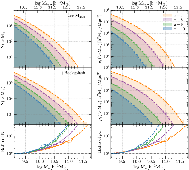
Figure 2: Cumulative distributions of halo mass $M_{\rm halo}$ of halos and stellar mass $M_{*}$ of central galaxies. The left column shows the cumulative number in the entire simulation volume of ELUCID, while the right column shows the cumulative stellar mass density. In the first row, the bound dark matter mass of the central subhalo is used, while in the second row, the mass brought in by backsplash halos is added. The third row shows the ratio of the number/mass density with added backsplash mass to that without backsplash mass. In each panel, solid lines are obtained from simulated halos, while dashed lines are obtained by fitting with Schechter functions. Results at $z=7$, $8$, $9$ and $10$ are shown by different colors as indicated in the top-right corner. A star formation efficiency $\epsilon_{*}=0.5$ is assumed in the conversion from halo mass to stellar mass. The significant enhancement in the number and mass densities at the high-stellar-mass end has non-negligible implications in the interpretation of the observed summary statistics. For further details, refer to §3.1.

The top-left panel of Fig. 1 shows a sample of halos with $M_{\rm halo}\geqslant 2\times 10^{11}\,h^{-1}{\rm M_{\odot}}$ at $z=8$ in a slice of the simulation box. At this redshift, there are already a large number of massive halos. Assuming a large but reasonable star formation efficiency, $\epsilon\sim 0.5$, these halos are capable of hosting massive galaxies with $M_{*}\gtrsim 10^{10}\,h^{-1}{\rm M_{\odot}}$ that have been identified by JWST (e.g., Rodighiero et al., 2022; Labbé et al., 2023). The two panels in the first row of Fig. 2 show the cumulative number density, $N(>M_{*})$, and the cumulative cosmic stellar mass density, $\rho_{*}(>M_{*})$, respectively, as functions of $M_{*}$ for galaxies in the entire simulation volume of ELUCID at snapshots from $z=7$ to $10$, with $M_{*}$ obtained by assuming a constant star formation efficiency $\epsilon_{*}=0.5$. More than 1000 galaxies with $M_{*}\geqslant 10^{10}\,h^{-1}{\rm M_{\odot}}$ can be found in the entire volume of ELUCID. In the following section, we examine whether or not the number of massive objects observed by JWST can be accommodated by the simulation.

3 Quantifying Uncertainties in Galaxy Counting

3.1 Expected Uncertainties from Different Sources

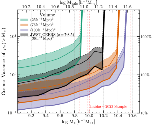
Figure 3: Cosmic variance on cumulative cosmic stellar mass density, $\rho_{*}(>M_{*})$, at $z=8$ estimated from the ELUCID simulation. Colored lines show the cosmic variance in boxes with given volumes indicated in the top-left corner, while black lines show the cosmic variance in a volume whose size and shape are consistent with the JWST CEERS program at $z=7$-$8.5$. For each case, thick solid, thin solid and dashed lines represent the $1$, $2$, and $3\,\sigma$ uncertainties, respectively, due to cosmic variance, which are obtained by randomly drawing 1000 subvolumes from the ELUCID simulation. The fractional value is labeled on the left axis, while the percentage value is labeled on the right axis. Vertical red dashed lines indicate the masses at which $\rho_{*}(>M_{*})$ is measured by Labbé et al. (2023) using the JWST CEERS sample consisting of four massive galaxies. A star formation efficiency $\epsilon_{*}=0.5$ is assumed in the conversion from halo mass to stellar mass. These results suggest significant mass dependence of cosmic variance and its capability to boost the spatial density of high-mass-end galaxies by more than an order of magnitude. For further details, refer to §3.1.

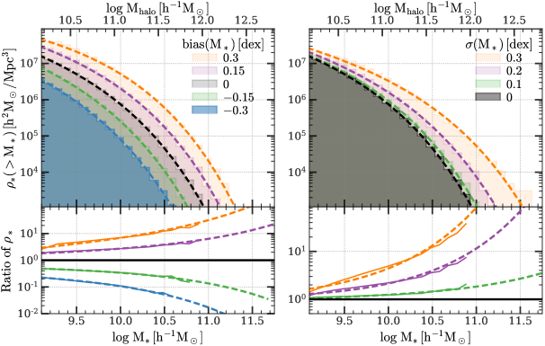
Figure 4: The impact of systematic and random errors in measuring stellar mass on cosmic stellar mass density. The left column represents different systematic biases assumed and indicated in the upper right corner, while the right column represents different random errors assumed and indicated in the upper right corner. The first row displays the cumulative cosmic stellar mass density, while the second row shows the ratio of the density with systematic/random error to that without error. Solid lines are obtained from simulated halos, while dashed lines are obtained by fitting with Schechter functions. All results are derived from ELUCID at $z=8$. A star formation efficiency $\epsilon_{*}=0.5$ is assumed in the conversion from halo mass to stellar mass. These findings highlight the importance of accurately estimating stellar mass to measure the abundance of massive galaxies. For further details, refer to §3.1.

Using the halo-to-galaxy transformations defined in the previous section, we now quantify the effect of their uncertainties on the estimate of the stellar mass density, $\rho_{*}(>M_{*})$. We first describe the effect of each uncertainty separately by zeroing out the other uncertainties. We then combine them to see their synergistic effect.

The second and third rows of Fig. 2 show the effect of mass enhancements introduced by backsplash halos on the transformation $\mathcal{T}_{M_{\rm halo}}$, where the “effective halo mass” is used to predict the stellar mass in it. To compare the results at the massive end, where the number/mass density drops down to the limit of the simulation, we fit the histogram with a Schechter function and extrapolate it to higher mass. Compared with the results without backsplash, the $N(>M_{*})$ or $\rho_{*}(>M_{*})$ for galaxies with $M\lesssim 10^{9}\,h^{-1}{\rm M_{\odot}}$ do not change. However, the effect of backsplash is more significant for galaxies of higher mass. The density can reach $\sim 200\%$ of its original value at $M_{*}\sim 10^{10}\,h^{-1}{\rm M_{\odot}}$ for all redshifts shown, and go beyond $1000\%$ at the high-mass end. This mass-dependency of the backsplash enhancement is the consequence of two effects. The first is that more massive halos are, on average, embedded in denser environments where high-speed close encounters are more frequent and the fraction of mass brought in by backsplash halos is higher. Second, the Schechter function for halo mass distribution declines exponentially at the high-mass end, so that the change in the halo mass is magnified in the halo mass function. It is not yet clear whether or not the baryon component of a backsplash halo can be effectively acquired by the host halo after the dark matter component is ejected, and whether or not the acquired gas can form stars effectively. Future detailed hydrodynamic simulations are needed to clarify the ambiguity.

Fig. 3 shows the effect of cosmic variance (CV) on $\rho_{*}(>M_{*})$ introduced by the sub-sampling operator $\mathcal{T}_{\rm CV}$:

$$CV(\rho_{*}|p)=\frac{\rho_{*,0.5(1+p)}}{\rho_{*,0.5}}-1.$$ (3)

Here, $p\in[0,1]$ is the target fraction of the probability mass centralized at the median, $\rho_{*,0.5(1+p)}$ is the quantile at the percentile $0.5(1+p)$, and $\rho_{*,0.5}$ is the median. We deliberately avoid using the average and standard deviation in the measurement of error, as they are not stable nor informative for a highly skewed distribution.

Throughout this paper, we use 1, 2 and 3$\sigma$ to denote cases where $p=0.68$, $0.95$ and $0.99$ are used for the quantiles, respectively. The distribution of $\rho_{*}$ is obtained numerically by sub-sampling the periodic box of ELUCID with a given volume, and the quantiles are estimated from the distribution. Here, we take the $z=8$ snapshot as an example and show CV for different volumes and for different thresholds of $M_{*}$. Solid, dashed, and dotted colored lines in Fig. 3 show 1, 2, and 3$\sigma$ CVs for a cubic volume of a given size. For low-mass galaxies with $M_{*}\sim 10^{9}\,h^{-1}{\rm M_{\odot}}$, the $1\sigma$ CV is estimated to be about $10\%$ for a volume of $(100\,h^{-1}{\rm{Mpc}})^{3}$ and increases monotonically to $\sim 70\%$ for a volume of $(25\,h^{-1}{\rm{Mpc}})^{3}$. This is consistent with the results obtained from the cosmic variance estimator given by Chen et al. (2019) for low-$z$ samples. Black lines show the CV expected for JWST CEERS at $z=7-8.5$, assuming a $38\,{\rm arcmin}^{2}$ effective sky area as used by (Labbé et al., 2023). The sub-sampling in ELUCID is conducted using beam-shaped volumes with a size of $(36\,h^{-1}{\rm{Mpc}})^{3}$ and a tangential-to-normal aspect ratio of $12/342$. The 1, 2, and 3$\sigma$ CVs are estimated to be $25\%$, $60\%$, and $80\%$ for low-mass galaxies. The moderate effect of CV on this mass scale indicates that the density of $M_{*}\lesssim 10^{9}\,h^{-1}{\rm M_{\odot}}$ galaxies can be estimated reliably in JWST CEERS if other uncertainties are well controlled.

However, the effect of CV has a significant dependence on stellar mass, with uncertainty reaching $100\%$ at higher stellar masses and eventually becoming divergent at the highest-mass end, regardless of the survey volume. The point of divergence shifts rightward as the volume increases, as it emerges when the median of $\rho_{*}(>M_{*})$ approaches zero. In Fig. 4, the vertical lines represent the masses at which $\rho_{*}(>M_{*})$ is measured by Labbé et al. (2023) using the four massive galaxies from JWST CEERS. Three of these lines intersect with the black solid line at CV $\sim 100\%$, suggesting that the CV is a significant effect for this small sample. The rightmost line, obtained from a galaxy with the most extreme stellar mass of $10^{10.89}{\rm M_{\odot}}$ at $z\sim 7.48$, is located in the divergent region of CV, indicating an incredible effect of uncertainty in the statistics drawn from this single galaxy. Since the divergence of CV is tightly related to the vanishing of the median $\rho_{*}(>M_{*})$ by its definition, it is more informative to model $\rho_{*}(>M_{*})$ forwardly, by directly predicting the distribution $P[\rho_{*}(>M_{*})]$ and the probability of observing a value of $\rho_{*}(>M_{*})$. We will demonstrate this later in this section.

Figure  4 illustrates the impact of the uncertainty in the stellar mass estimator, $\mathcal{T}_{M_{*}}$. To demonstrate the effect, we take all halos at the $z=8$ snapshot of ELUCID as an example. In the left panel, we show the change of $\rho_{*}(M_{*})$ when different levels of systematic error i.e. bias, are added to the stellar mass predicted by Eq. 2. A negative (positive) bias naturally decreases (increases) $\rho_{*}(M_{*})$, as it is equivalent to a lower-left (upper-right) shift of the distribution function. However, when considering the ratio of the biased distribution to the unbiased one, a stellar-mass dependency is observed. This is similar to the mass dependency of CV, where a small perturbation to the transformation is magnified significantly owing to the steepness of the Schechter function at the high-stellar-mass end. The overall outcome is an increased effect of the uncertainty in the stellar mass estimate at the high-mass end, and a divergence occurs when the unbiased galaxy number $N(>M_{*})$ approaches zero.

In the right panel of Fig. 4, we show the effect of random error, known as the Eddington bias (Eddington, 1913), in the stellar mass estimate. Here, we model the error as a Gaussian random variate with zero mean and varying standard deviation, $\sigma_{M_{*}}$. Lines with different colors represent results with different $\sigma_{M_{*}}$, and are compared to the result assuming no error. Once again, to enable a comparison in the full mass range, we fit the histogram to a Schechter function and extrapolate it to the uncovered mass range. As the distribution of $M_{*}$ has a negative derivative, a symmetric noise in $M_{*}$ produces an asymmetric effect on the number counts of galaxies. As the derivative becomes more negative toward the high-stellar-mass end, the effect of this type of noise becomes more significant. We do see this expected behavior in the panel, where the histogram is lifted everywhere by a nonzero error of $M_{*}$. With a moderate random error of 0.2 dex (0.3 dex), the increase of $\rho_{*}(M_{*})$ is $\sim 100\%$ at $M_{*}\sim 10^{9.2}\,h^{-1}{\rm M_{\odot}}$ ($10^{9.7}\,h^{-1}{\rm M_{\odot}}$), and becomes divergent when the number of galaxies $N_{>M_{*}}$ approaches zero.

As suggested by Lovell et al. (2022) and Boylan-Kolchin (2023), an assumption of $\epsilon_{*}\sim 1$ still results in a $\sim 3\sigma$ tension in $\rho_{*}(>M_{*})$ with recent JWST observations, especially when the massive galaxies at $z=7-10$ from the JWST CEERS sample (Labbé et al., 2023) are included. With all the uncertainties introduced above, and the fact that all of them have a strong effect on the statistics drawn from samples of small size, it is likely that the observational results can be reproduced by the theory with much less tension, as demonstrated in the following.

3.2 Implications for JWST Observations

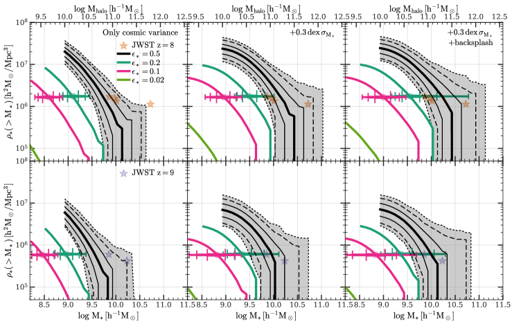
Figure 5: A comparison of the cumulative cosmic stellar mass density at $z=8$ (first row) and $z=9$ (second row) with the results obtained from the JWST CEERS sample (Labbé et al., 2023). The different uncertainties, including cosmic variance, random error in measuring stellar mass, and the mass enhancement by backsplash systems, are incrementally added and shown from left to right columns. In each panel, the thick solid line represents the median, while the thin solid, dashed and dotted lines represent the 1, 2, and 3 $\sigma$ ranges, respectively, of the stellar mass density. The volume used in the estimate of cosmic variance is chosen to be consistent with the CEERS sample at the corresponding redshift. For black lines, a star formation efficiency of $\epsilon_{*}=0.5$ is assumed in the conversion from halo mass to stellar mass (refer to §2 for details). For references, the colored curves show the results obtained by assuming $\epsilon_{*}=0.2$, $0.1$, and $0.02$, respectively. The horizontal error bars indicate the 1, 2, and 3 $\sigma$ ranges at the stellar mass density corresponding to the leftmost observational data point in the same panel. These results suggest that the observed high-mass sample in the recent JWST survey can be safely covered by $2\sigma$ with a reasonable star formation efficiency of $\epsilon_{*}=0.5$. The inclusion of backsplash halos may further reduce the tension to $\sim 1\sigma$. For further details, refer to §3.2.

Fig. 5 shows the cumulative cosmic stellar mass density $\rho_{*}(M_{*})$ as a function of the limiting stellar mass $M_{*}$ for two different redshifts, $z\sim 8$ and $z\sim 9$, where six extremely massive galaxy candidates are identified and $\rho_{*}(>M_{*})$ estimated by Labbé et al. (2023). We demonstrate effects of different sources of uncertainties by incrementally adding them into the transformations, $\mathcal{T}_{\rm CV}$, $\mathcal{T}_{\rm M_{halo}}$, and $\mathcal{T}_{\rm M_{*}}$, respectively, in the mapping from halo sample, $S_{\rm halo}$, to the galaxy statistic, $\rho_{*}(>M_{*})$, as introduced in §2.2. The JWST detections are overplotted for comparison.

Black lines with gray shading in the left column of Fig. 5 show the median and different $\sigma$ ranges derived from the probability distribution $P[\rho_{*}(>M_{*})|M_{*}\,,\epsilon_{*}=0.5\,,{\rm CV}]$ when cosmic variance is incorporated by volume sub-sampling and a star formation efficiency $\epsilon_{*}=0.5$ is adopted to convert halo mass to stellar mass. The results shown here are consistent with those obtained by Lovell et al. (2022) and Boylan-Kolchin (2023) that some data points are outside the $\sim 3\sigma$ range. The exact tension level is slightly different, likely because of their simplification in the error calculation with analytical approximations, the difference in the cosmologies adopted, and the difference in the version of galaxy data. The point obtained by us from a $z\sim 8$ extreme is the only one that lies outside the $3\sigma$ range, while the $z\sim 9$ extreme marginally touches the $2\sigma$ boundary. Other points are all contained within the $2\sigma$ boundary.

As demonstrated in §3.1 and §4, Eddington bias is able to lift the galaxy number by more than an order of magnitude, which may help explain the outliers we see here. The middle column of Fig. 5 shows the probability distribution $P[\rho_{*}(>M_{*})|M_{*},\,\epsilon_{*}=0.5,\,{\rm CV},\,{\rm\sigma_{M_{*}}}=0.3\,{\rm dex}]$ when a Gaussian random error with a conservative 0.3 dex standard deviation is added to the estimate of $\log\,M_{*}$. A significant shift of the median $\rho_{*}(>M_{*})$ and a significant broadening of the quantile ranges can be seen after the incorporation of this uncertainty. The $z=8$ extreme is now safely contained within the 2$\sigma$ range of $\rho_{*}(>M_{*})$, and all the $z=9$ points are contained by the $1\sigma$ range. Thus, once the cosmic variance and the Eddington bias are included, there is no significant tension between the $\Lambda$CDM paradigm and the JWST observations, if the star formation efficiency can reach $0.5$ at these redshifts.

The right column of Fig. 5 shows the results for $\rho_{*}(M_{*})$ when the third source of uncertainty, the backsplashed mass, is taken into account and added into the halo mass estimator, $\mathcal{T}_{M_{\rm halo}}$. Unlike cosmic variance and random error in the stellar mass estimate, this effect always increases halo mass and thus provides a larger effective baryon mass for star formation. The outcome is obvious: all the data points at $z\sim 8$ and $9$ are now below the upper $2\sigma$ quantile once a star formation efficiency $\epsilon_{*}=0.5$ is assumed. At $z\sim 8$, three of the four data points actually lie close to the lower $2\sigma$ quantile, while the most massive is close to the upper $1\sigma$ quantile.

The colored curves in Fig. 5 show the results obtained by considering lower star formation efficiencies, $\epsilon_{*}=0.2$, $0.1$, and $0.02$, which are more realistic expected from low-z observations. Each curve is overplotted with a series of horizontal error bars, which indicate the $1\sigma$, $2\sigma$, and $3\sigma$ ranges at the stellar mass density corresponding to the leftmost observational data point in the same panel. When solely considering cosmic variance and assuming $\epsilon_{*}=0.2$, none of the observational data points fall within the $3\sigma$ ranges. However, when introducing a standard deviation of 0.3 dex to the estimate of $\log,M_{*}$, the leftmost data points for both the $z=8$ and $z=9$ observations fall within the $3\sigma$ range. Furthermore, when incorporating the backsplash effect, these observations shift into the $2\sigma$ ranges. These findings suggest that a star formation efficiency of $\epsilon_{*}=0.2$ can marginally account for the high stellar mass densities obtained from the CEERS sample. Nevertheless, when considering more common values for the low-z Universe, for example, $\epsilon_{*}=0.1$ and $\epsilon_{*}=0.02$ (e.g., Yang et al., 2003; Moster et al., 2010; Yang et al., 2012; Reddick et al., 2013; Behroozi et al., 2013; Moster et al., 2013; Birrer et al., 2014; Lu et al., 2014; Rodríguez-Puebla et al., 2017; Shankar et al., 2017; Moster et al., 2018; Behroozi et al., 2019), the modeled stellar mass densities do not reach the observational values. This indicates that a simple extrapolation of low-z observations is insufficient in explaining the CEERS observations.

All the results presented above highlight the importance of fully modeling all the uncertainties when interpreting the observational data. Since each of the three sources of uncertainty considered above has a positive effect on $\rho_{*}(>M_{*})$, a lower star formation efficiency $\epsilon_{*}$ is needed to explain the observed data when the uncertainty involved is larger. Conversely, a greater $\epsilon_{*}$ is necessary to explain the observational data if the uncertainty is smaller. Since the exact level of uncertainty in each transformation step is not known a priori, we provide a general prediction for the relationship between the level of uncertainty and the probability to accommodate the observational data. For a given observed density, $\rho_{*,{\rm obs}}(>M_{*})$, we define the probability to observe it as the remaining probability mass of having $\rho_{*}(>M_{*})>\rho_{*,{\rm obs}}(>M_{*})$:

$$p_{\rm obs}=1-\left.{\rm CDF}[\rho_{*}(>M_{*})]\right|_{\rho_{*}(>M_{*})=\rho_{*,{\rm obs}}(>M_{*})},$$ (4)

where ${\rm CDF}[\rho_{*}(>M_{*})]$ is the cumulative distribution function of $\rho_{*}(>M_{*})$ derived from $P[\rho_{*}(>M_{*})]$. This probability can be used to obtain the level of uncertainties and the star formation efficiency required to explain the observation.

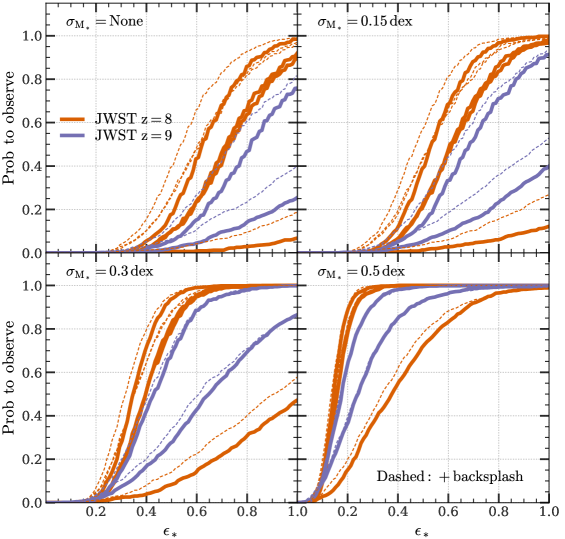
Figure 6: The probability of obtaining the cosmic cumulative stellar mass density, $\rho_{*}(>M_{*})$, as measured from the six extremely massive galaxies of the JWST CEERS sample (Labbé et al., 2023). The probability is plotted as a function of the star formation efficiency, $\epsilon_{*}$, used in the conversion from halo mass to stellar mass. Each panel displays the result for a given random error in the estimate of stellar mass, $\sigma_{M_{*}}$, which is indicated in the upper left corner of that panel. The volume of sub-boxes used to estimate the probability is chosen to be consistent with the JWST CEERS sample at the corresponding redshift, as indicated in the first panel. The solid lines are obtained using simulated halo mass, while the dashed lines are obtained by adding the mass due to backsplash halos. For futher details, refer to §3.2.

Fig. 6 displays the predicted $p_{\rm obs}$ for the six data points obtained by Labbé et al. (2023) as a function of star formation efficiency $\epsilon_{*}$, taking into account different sources of uncertainty. The upper left panel shows the case that does not include the random error in the stellar mass estimator. Without mass added by backsplash halos, four of the samples have $p_{\rm obs}>10\%$ for $\epsilon_{*}=0.5$. However, one extreme at $z\sim 8$ has $p_{\rm obs}<10\%$ even for $\epsilon_{*}=1$, suggesting a possible tension. With the backsplash effect included, the $p_{\rm obs}$ value is three times the original value at $\epsilon_{*}=1$ for this extreme, and it is non-zero at $\epsilon_{*}=0.5$. A random error with $\sigma_{\rm M_{*}}$ ranging from $0.15\,{\rm dex}$ to $0.3\,{\rm dex}$ on the stellar mass estimate increases the probability further. A $\sigma_{M_{*}}$ of 0.5 dex drastically changes the trend of $p_{\rm obs}$; even $\epsilon_{*}=20\%$ is sufficient to move all the observed samples to within the $1\sigma$ range ($p_{\rm obs}\geqslant 0.16$).

It is important to note that the probability prediction presented here is based solely on empirical modeling of uncertainties in the $\Lambda$CDM cosmology. Therefore, the results are quite general and can be extended to other surveys, regardless of the details of the survey strategy, data processing and statistical model. However, further work is needed to confirm conjectures presented here. Surveys with large areas are useful in suppressing cosmic variance and thus in reducing the uncertainty in volume sampling. Hydrodynamic simulations and semi-analytical modeling are needed to verify or rule out the proposed effect of backsplash, as well as to understand the conversion of baryons to stars. Deeper imaging, high S/N spectroscopy, and precise stellar population synthesis are critical in order to narrow down the posterior parameter space in the estimates of redshift and stellar mass estimate. All these, together, may eventually resolve the tension or provide definitive evidence for the need of new cosmology and new physics.

4 Descendants of High-redshift Massive Galaxies

Within the scope of data and models currently available, it is interesting to explore how the observed massive galaxies would evolve over the cosmic history and where they end up in the local universe. Answers to these questions may provide hints for searching for descendants of these high-$z$ massive galaxies.

4.1 Mass Distribution of Descendant Halos

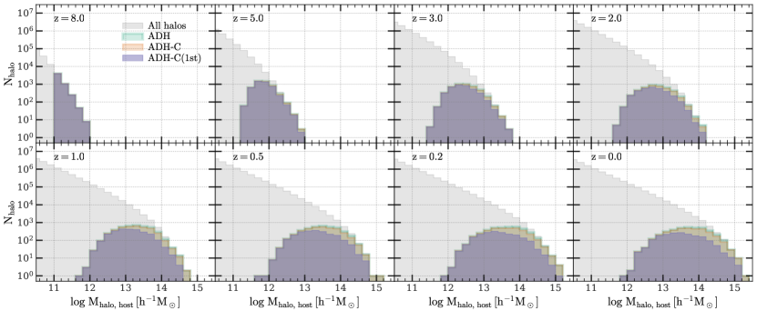
Figure 7: Histograms of the halo mass, $M_{\rm halo,host}$, for ancient descendant halos (ADH) of a sample of the most massive galaxies, $S$, selected with $M_{\rm halo,host}\geqslant 10^{11}\,h^{-1}{\rm M_{\odot}}$ at redshift $z_{\rm g}=8$ from ELUCID. In each panel, the colored histograms represent different types of ADH with incremental constraints. The green histogram labeled as “ADH” includes any halo that hosts at least one descendant subhalo, whether in central or satellite, of a galaxy in $S$. The brown histogram labeled as “ADH-C” includes any halo whose central subhalo is a descendant of a galaxy in $S$. The purple histogram labeled as “ADH-C(1st)” includes any halo whose central subhalo is the first descendant of a galaxy in $S$. For comparison, the histogram for all halos at each snapshot is shown in black. The results suggest that most of the ancient stars formed in the most massive halos at $z_{\rm g}\sim 8$ will eventually reside in the massive halos with $M_{\rm halo,host}\gtrsim 10^{13}\,h^{-1}{\rm M_{\odot}}$. For further details, refer to §4.1.

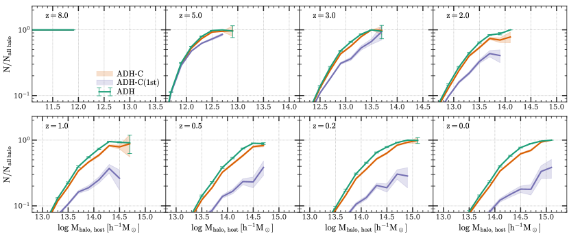
Figure 8: The proportions of various types of ancient descendant halos (ADH) of a sample of the most massive galaxies at redshift $z_{\rm g}=8$. These proportions are obtained by calculating the ratios of the colored histograms in each panel of Fig. 7 to the black histogram. The mean fraction is represented by the solid line, while the shaded area or error bar indicates the standard deviation, which is computed from 100 bootstrapped samples. For further details, refer to §4.1.

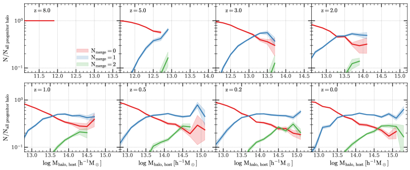
Figure 9: The proportion of $z_{\rm g}=8$ massive galaxies that enter the central subhalos of their ancient descendant halos (ADH) at lower $z$, with different numbers of mergers, denoted as $N_{\rm merge}$. The result for each given $N_{\rm merge}$ is represented by a different color. The halo mass, $M_{\rm halo,host}$, of ADH is labeled on the x-axis. The solid line represents the mean fraction, while the shaded area indicates the standard deviation, which is computed from 100 bootstrapped samples. For further details, refer to §4.1.

In order to investigate the properties of the descendants of high-redshift massive galaxies, we use subhalo merger trees in the ELUCID simulation. This enables us to establish a connection between the high-redshift galaxies, as predicted by our empirical transformations in §2.2, and low-redshift halos which host the descendants of these galaxies. For convenience these low-$z$ halos are referred to as “ancient descendant halos”, or “ADH” for short. Note that ADH are defined at a given redshift, $z$, for galaxies modeled at a higher redshift, $z_{\rm g}$. We study both the spatial and mass distribution of these ADH. It is important to note that the density field of ELUCID is constrained by real observations, as outlined in §2.1. Thus, the connection established can also be used to understand the formation history of real massive clusters in the local universe back to a time when the universe was only approximately 500 million years old.

The green histograms in Fig. 7 depict the distribution of mass, $M_{\rm halo,host}$, for the ADH of high-$z_{\rm g}$ massive galaxies. In this section, we use the top-hat mass for halos, since it is easier to infer from observation and since we are conducting statistics for a halo as a whole (e.g., Yang et al., 2007; Yang et al., 2012; Lim et al., 2017; Tinker, 2020; Yan et al., 2020; Wang et al., 2020; Hung et al., 2021). We select high-$z_{\rm g}$ galaxies as the central galaxies in the most massive halos with $M_{\rm halo,host}\geqslant 10^{11}\,h^{-1}{\rm M_{\odot}}$ at $z_{\rm g}=8$ in the entire ELUCID volume. From $z=8$ to $z=0$, the descendant halos of these massive high-redshift galaxies are found preferentially in the massive end of the mass distribution of the total population (the black histogram), although the distribution can extend to masses as low as $\sim 10^{12}\,h^{-1}{\rm M_{\odot}}$. At the massive end of the histogram, almost all halos are ADH of massive galaxies at $z_{\rm g}=8$. The minimum mass of the descendant halo is approximately $10^{11.5}\,h^{-1}{\rm M_{\odot}}$ ($10^{12}\,h^{-1}{\rm M_{\odot}}$) at $z=2$ ($z=0$), while the median is around $10^{12.8}\,h^{-1}{\rm M_{\odot}}$ ($13.5\,h^{-1}{\rm M_{\odot}}$). However, among the total population of halos at $z=0$ with $M_{\rm halo}\sim 10^{13.5}\,h^{-1}{\rm M_{\odot}}$, only about $10\%$ are ADH of massive galaxies at $z_{\rm g}=8$, and the fraction drops exponentially towards lower halo masses.

To quantify the precise fraction of high-$z_{\rm g}$ massive galaxies that end up in low-$z$ halos of different masses, we present the ratio between the ADH mass histogram with the unconditional halo-mass histogram at different redshift, $z$, in Fig. 8 using the same green color as in Fig. 7. The shaded area attached to each curve represents the standard deviation estimated from 100 bootstrapped samples. A halo with a mass of $10^{14}\,h^{-1}{\rm M_{\odot}}$ ($10^{15}\,h^{-1}{\rm M_{\odot}}$) at $z=2$ ($z=0$) almost certainly contains at least one descendant of the most massive galaxies at $z_{\rm g}=8$, while a halo with a mass of $10^{13.5}\,h^{-1}{\rm M_{\odot}}$ ($10^{14.5}\,h^{-1}{\rm M_{\odot}}$) has a probability of $\gtrsim 70\%$ to do so. For halos with a mass of $10^{13}\,h^{-1}{\rm M_{\odot}}$ ($10^{13.5}\,h^{-1}{\rm M_{\odot}}$), the probability drops to $\lesssim 30\%$. Note that we do not differentiate between centrals and satellites in descendant halos.

The brown histograms labeled as “ADH-C” in Fig. 7 represent the number of ADH that contain the descendant galaxies as their central galaxies. The lines in Fig. 8 show the fraction of these halos among the total population at the same redshift. The similar values of the green (ADH) and brown (ADH-C) histograms/lines suggest that most of the high-$z_{\rm g}$ massive galaxies eventually become the dominant galaxies or parts of the dominant galaxies of massive halos at low-$z$. Due to hierarchical formation of galaxies in the $\Lambda$CDM model, some of the high-$z_{\rm g}$ massive galaxies become parts of more dominating centrals at low-$z$ while others remain as the dominating centrals. To demonstrate this, the purple histograms and lines in Fig. 7 and Fig. 8, marked as “ADH-C(1st)”, represent the number and fraction, respectively, for low-$z$ halos whose central subhalos are the first descendants of the $z_{\rm g}=8$ massive galaxies. Here, a subhalo A is considered to be the first progenitor of another subhalo B in the subsequent snapshot, if A has the greatest bound mass among all of B’s progenitors. In this case, we refer to B as the first descendant of A, only to make clear the special status of A. In addition, the chain of first progenitors (i.e., the main branch) of B can be determined by recursively identifying the first progenitor along the links in the tree towards higher redshift. Thus, ADH-C(1st) at a given $z$ are halos at $z$ that each has a massive progenitor galaxy at $z_{\rm g}$ in the main branch of its central subhalo. The results indicate that approximately $30\%-40\%$ of the central galaxies in the most massive halos at low-$z$ halos are direct descendants of the most massive, high-$z_{\rm g}$ galaxies.

The findings presented here provide a compelling guidance regarding the sites to identify remnants of the old stellar population formed at high-$z$. For instance, since central galaxies in the majority of massive clusters with $M_{\rm halo}\sim 10^{14}\,h^{-1}{\rm M_{\odot}}$ ($10^{15}\,h^{-1}{\rm M_{\odot}}$) at $z=2$ ($z=0$) are highly likely to contain ancient stars from $z\sim 8$, targeting the central galaxies of these potential ADH with infrared spectroscopic observations might reveal the presence of this ancient stellar population. This, in turn, would facilitate comparisons with stellar populations that formed later to investigate star formation in high-$z$ galaxies.

In Fig. 9, we partition the $z_{\rm g}=8$ galaxy sample, whose descendants are centrals at some lower redshift (indicated by orange symbols in Fig. 7 and Fig. 8), into subsets based on $N_{\rm merge}$, the number of mergers they underwent before entering the central galaxies of their ADH. Note that here we only include merger events in which the subhalo under consideration was the less-massive one in the encountering subhalos. The fractions of galaxies in these subsets as a function of host halo mass are depicted by lines and shadings of different colors for different redshifts below $z=8$. The fraction of galaxies with $N_{\rm merge}=0$ consistently declines with increasing host halo mass at all redshifts. This is because a host halo with greater mass harbors more satellites, thereby increasing the likelihood of close encounters among its satellites. The proportion of galaxies with $N_{\rm merge}=1$ or $2$ steadily increases with host halo mass at all redshifts. At the high-mass extreme, galaxies with $N_{\rm merge}=1$ emerge as the dominant population, indicating that most central galaxies in the most massive halos at lower redshifts have undergone at least one merger event in their history. As redshift decreases, the $N_{\rm merge}=2$ cases become increasingly prevalent, eventually outnumbering the $N_{\rm merge}=0$ case.

Given that the galaxies we have chosen at $z_{\rm g}=8$ are the most massive ones at that time, it is highly probable that the merger events in which they entered the central galaxies of their ADH were all major ones. These major mergers can cause angular momentum loss, black hole growth, morphology transformation, and quenching of galaxies. Our findings thus imply that the central galaxies in local massive halos underwent one or two bursts in star formation. These outcomes may serve as valuable priors for Bayesian spectral synthesis models (e.g., Zhou et al., 2019; Johnson et al., 2021), where one or more burst components can be incorporated into the star formation history.

The significant spread of the $M_{\rm halo,host}$ distribution for ADH at $z\lesssim 5$ shown in Fig. 7, coupled with the diverse merger histories of the descendants of high-$z_{\rm g}$ massive galaxies shown in Fig. 9, implies a disruption of the rank order for halo/stellar mass during the evolution. Consequently, abundance matching between progenitors and descendants using only halo and stellar mass may not be accurate, thus presenting a problem for rank-based empirical methods to link galaxies between different redshifts (e.g., Zheng et al., 2007; Behroozi et al., 2019; Wang et al., 2023b; Zhang et al., 2022a). Our findings suggest that these methods need to be improved, and that the inclusion of secondary halo properties might be needed. We also note that some efforts have been made to identify proto-clusters at intermediate redshifts ($1\lesssim z\lesssim 3$) and use them to establish a statistical link between galaxies at different redshifts (e.g., Chiang et al., 2013, 2014; Cai et al., 2016, 2017; Wang et al., 2021). With ongoing and future surveys, these methods can be extended and applied to high-$z$ data. This will open a new avenue to study the evolution of the galaxies across the history of the universe.

4.2 Assembly History of Individual Clusters

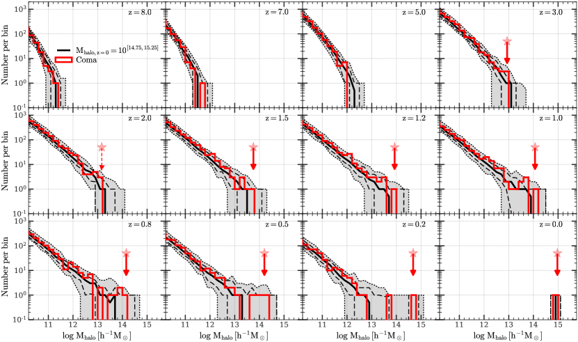
Figure 10: The progenitor halo mass functions at different redshifts, shown in different panels, of massive halos at $z=0$. The black histograms in each panel correspond to the $z=0$ halos with $10^{14.75}\leqslant M_{\rm halo}/(\,h^{-1}{\rm M_{\odot}})\leqslant 10^{15.25}$. The solid, dashed and dotted lines indicate the median, $1\sigma$, and $2\sigma$ ranges of the histograms at a given halo mass, respectively. The red histogram represents the Coma cluster, while the red arrow indicates the host halo mass of the first progenitor (main branch) subhalo of the central subhalo of Coma, solid if the progenitor is a central subhalo and dashed if it is a satellite. These results reveal an unusual formation history of Coma, whose mass was mostly assembled at $z\lesssim 2$ due to violent merges. For further details, refer to §4.2.

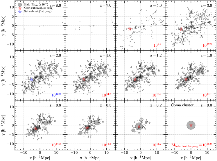
Figure 11: The spatial distribution of progenitor halos of the Coma cluster at different redshifts, shown in different panels, as simulated by ELUCID. In each panel, each black circle represents one progenitor halo with halo mass $M_{\rm halo}\geqslant 10^{11}\,h^{-1}{\rm M_{\odot}}$. The size of circle is set according to halo mass. The star symbol marks the location of the first progenitor (main branch) subhalo of the central subhalo of Coma, shown in red if it is a central subhalo and blue if it is a satellite. The host halo mass of the first progenitor subhalo is indicated in the lower-right corner of each panel. For further details, refer to §4.2.

The diversity of the descendant distribution highlights the need to investigate the evolution of individual galaxy clusters in the low-$z$ universe. In this section, we present the assembly histories of selected halos that can be matched to real clusters of galaxies, capitalizing on ELUCID with its nature of being constrained by the galaxy distribution in the SDSS survey.

Coma is a massive cluster located in the nearby universe, positioned at $({\rm RA}$, ${\rm Dec}$, ${\rm z_{\rm CMB}})$ $=(194.95^{\circ}$, $27.98^{\circ}$, $0.0231)$. According to Yang et al. (2007); Yang et al. (2012), its estimated halo mass is about $9.3\times 10^{14}\,h^{-1}{\rm M_{\odot}}$. In ELUCID, the matched halo is located at $(194.81^{\circ}$, $27.91^{\circ}$, $0.0240)$ and has a halo mass of $9.4\times 10^{14}\,h^{-1}{\rm M_{\odot}}$. In Fig. 1, we follow a halo with $M_{\rm halo}$ slightly larger than $10^{11}\,h^{-1}{\rm M_{\odot}}$ at $z=8$ (top-left panel), which joins the Coma cluster at $z=0$ (lower-right panel). Note that this halo is actually not the most massive one at $z=5$, $3$ and $1.5$ among all the halos displayed in the same panels. Only at lower redshifts, $z=1.5$ and $0$, does Coma become the most massive cluster. This suggests an unusual characteristic of Coma, which formed relatively late, perhaps via violent mergers during later epochs.

To understand the evolution of Coma in more detail, Fig. 10 displays the mass distribution reconstructed by ELUCID for its progenitor halos, with a red arrow indicating the host halo mass, at each snapshot, of the first progenitor subhalo of the central subhalo of Coma at $z=0$. For comparison, we depict the median mass distribution, as well as the 1 and $2\sigma$ ranges, for progenitors of halos at $z=0$ with $10^{14.75}\leq M_{\rm halo}/(\,h^{-1}{\rm M_{\odot}})\leq 10^{15.25}$. At $z=8$, The most massive progenitor of Coma has $M_{\rm halo}\sim 2\times 10^{11}\,h^{-1}{\rm M_{\odot}}$, barely touches the high-mass end, as shown in the top-left panel of Fig. 7. At $z=0$, Coma has $M_{\rm halo}\approx 10^{15}\,h^{-1}{\rm M_{\odot}}$, which is at the high-mass end, as demonstrated in the lower-right panel of Fig. 7. At $z=5$, progenitors of Coma are less massive than the average for similarly massive halos at $z=0$. At $z=3$, the first progenitor of Coma forms, and at $z=2$, it merges with another halo and becomes a satellite. This suggests that the birthplace of Coma was in a crowded environment. At $z\leq 1.5$, the massive end of the distribution of Coma’s progenitor mass exceeds the average, and the overall amplitude of the distribution also goes above the average (as seen from the red and black solid histograms). At $z\leq 1$, several massive progenitors form and eventually merge with the first progenitor. All these suggest that violent mergers at $z\lesssim 3$, particularly at $z\leq 1$, played a critical role for Coma to assemble a large amount of mass by $z=0$.

In Fig. 11, we present the projected 2-D spatial positions of Coma’s progenitors. A star is used to mark the spatial location of the first progenitor subhalo, at each snapshot, of the central subhalo of Coma at $z=0$, shown in red if the progenitor subhalo is a central and blue if it is a satellite. The abundance of progenitors at $z\lesssim 5$ indicates the dense environment of Coma, where frequent mergers are taking place. This is in agreement with observations, such as those from SDSS (Abazajian et al., 2004), which report a substantial fraction of red galaxies in Coma (e.g., de Propris et al., 1998; Eisenhardt et al., 2007; Jenkins et al., 2007; Adami et al., 2009; Miller et al., 2009; Mahajan et al., 2010; Hammer et al., 2010; Mahajan et al., 2011; De Propris, 2017). At $z=0.5$, two massive structures are visible among the progenitors, consistent with the observed presence of two massive elliptical galaxies near the center of Coma. It is noteworthy that overall mass distribution of Coma is not spherically symmetric and that it is surrounded by filamentary structures that contribute to its continuous mass assembly. Future X-ray observations of these filaments may provide additional constraints on the environment and assembly history of the Coma cluster.

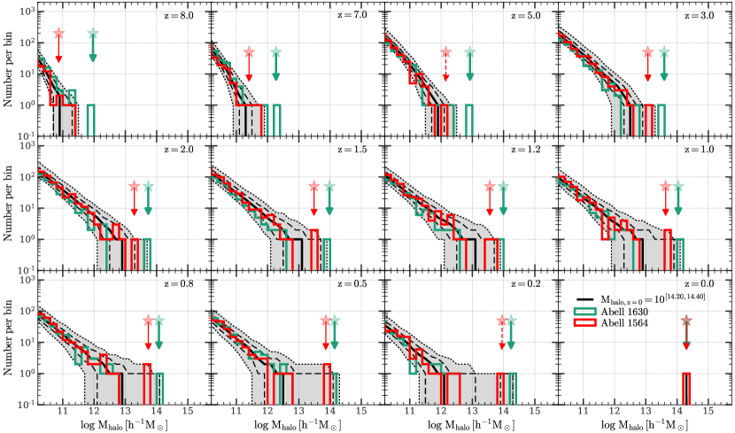
Figure 12: The same as Fig. 10 but for less massive $z=0$ halos with $10^{14.2}\leqslant M_{\rm halo}/(\,h^{-1}{\rm M_{\odot}})\leqslant 10^{14.4}$. Green and red histograms/arrows are for two $z=0$ clusters, Abell 1630 and Abell 1564, respectively. These results show two extremes of cluster formation, through equal-mass merger event (Abell 1564) or continuous accretion (Abell 1630).

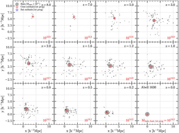
Figure 13: The same as Fig. 11 but for Abell 1630.

According to the extended Press-Schechter formalism (Lacey & Cole, 1993), the progenitor mass distribution is expected to depend on the mass of descendant halos. Fig. 12 depicts the progenitor mass distributions at various redshift for present-day halos in the mass range $10^{14.2}\leq M_{\rm halo}/(\,h^{-1}{\rm M_{\odot}})\leq 10^{14.4}$. The median, $1\sigma$, and $2\sigma$ ranges are displayed by solid, dashed and dotted lines, respectively. In addition, we also show the progenitor distributions for two $z=0$ halos matched with Abell 1630 and Abell 1564.

Abell 1630 is a galaxy cluster located at $({\rm RA}$, ${\rm Dec}$, ${\rm z_{\rm CMB}})$ $=(192.93^{\circ}$, $4.56^{\circ}$, $0.064)$, and its estimated halo mass is $1.78\times 10^{14}\,h^{-1}{\rm M_{\odot}}$ by Yang et al. (2007); Yang et al. (2012). In the ELUCID simulation, its position is simulated at $(193.18^{\circ},4.42^{\circ},0.064)$, and its halo mass is $2.01\times 10^{14}\,h^{-1}{\rm M_{\odot}}$. Abell 1630 is quite unique in that its first progenitor significantly dominates the progenitor population. The mass gap between the first and other progenitors is evident from $z=8$ and continues throughout its history until $z=0$. This suggests that Abell 1630 has assembled most of its mass through continuous accretion or relatively minor mergers, which is very different from Coma, where late-time major mergers dominate the mass assembly. This cluster has a massive progenitor at $z=8$, which lies well outside the $2\sigma$ range of the mass distribution and is even more massive than the most massive progenitor of Coma at the same redshift. These suggest that Abell 1630 should have a dominating member at $z=0$ near the center. Indeed, a luminous red galaxy with an absolute magnitude of $M_{\rm r}^{0.1}=-22.17$ and a color index of $(g-r)^{0.1}=0.93$ has been identified in this cluster, consistent with the expectation of ELUCID.

The spatial locations of the progenitors of Abell 1630 at different snapshots are displayed in Fig. 13. A comparison with the corresponding plot for Coma in Fig. 11 reveals that Abell 1630 formed in an environment with only a moderate matter density, which may be the cause of its assembly history distinctive from that of Coma.

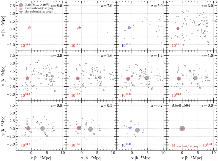
Figure 14: The same as Fig. 11 but for Abell 1564.

Abell 1564, the final example, is observed at $(188.74^{\circ}$, $1.84^{\circ}$, $0.0780)$. Its estimated halo mass is $2.87\times 10^{14}\,h^{-1}{\rm M_{\odot}}$, and it is reconstructed by ELUCID at $(188.96^{\circ}$, $2.02^{\circ}$, $0.0784)$ with a halo mass of $1.99\times 10^{14}\,h^{-1}{\rm M_{\odot}}$. The progenitor mass and spatial distributions are shown in Fig. 12 (the red histograms) and in Fig. 14, respectively.

The assembly history of Abell 1564 falls between the two extremes shown above in that it has gone through only one major merger in its entire history. The two merging progenitors at $z=0.5$ have nearly equal mass and, as a result, the first progenitor of Abell 1564 became a satellite subhalo during a short period of time at $z\sim 0.2$ after the merger. This late-time major merger implies that the cluster at $z=0$ may not yet be fully virialized. The non-spherical light distribution of Abell 1564 in real observations provides supports to our conclusion.

The three examples presented here illustrate three distinct assembly modes of massive clusters: one with multiple major mergers like Coma, one with only one major merger like Abell 1564, and one with continuous accretion (or minor mergers) like Abell 1630. To illustrate the differences between the modes, we present the mass assembly histories of the three clusters as a function of redshift in Fig. 15 for $M_{\rm halo,main\ branch}$, which is the mass of the main branch progenitor, $M_{\rm halo,total}$, which is the total mass contained in all progenitor halos with $M_{\rm halo}\geqslant 10^{10}\,h^{-1}{\rm M_{\odot}}$, and the ratio between them. Among the three clusters, Coma is the most massive at $z=0$, but its main progenitor is the least massive at $z\gtrsim 3$. Three faster growth stages at $z\sim 5$, $2$ and $0.5$ respectively, are clearly seen in the growth of Coma’s main branch, indicating violent merger events in its history. From Fig. 11, it is evident that these three fast accretion stages result from the richness of Coma’s progenitor halos and their asymmetric spatial distribution. The other extreme, Abell 1630, shows continuous growth of its main branch. It was massive enough to host a bright galaxy at $z\gtrsim 8$, but its main-branch mass assembly history is smooth and slow, culminating in a final halo less massive than Coma. The in-between case, Abell 1564, shows only one main-branch mass jump at $z\sim 0.5$, which results from the major merger event seen in Fig. 14. During most of its history, Abell 1564 has a main-branch-to-total ratio lying between the two extremes, Coma and Abell 1630. Note that in some cases during mergers, the curves of total mass even decrease. This is an artificial effect, due to the fact that some particles linked by the FoF algorithm are not enclosed in the "tophat" filter that defines the halo mass. The diversity of the formation mode, as represented by the main branch growth rate and the number of merger events, may be responsible for the significant variation observed in the descendant mass distribution in §4.1. Such variation must be carefully taken into account when constructing models to link galaxies over a wide range of redshifts.

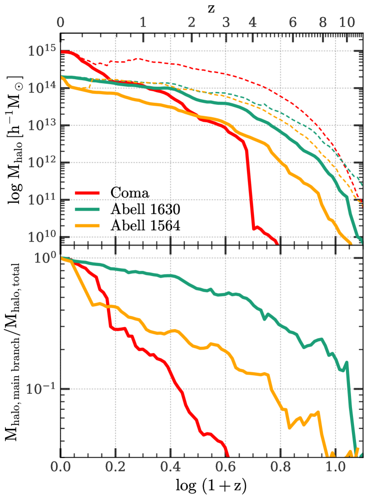
Figure 15: Mass assembly histories of Coma (red), Abell 1630 (green) and Abell 1564 (orange). In the upper panel, solid lines show $M_{\rm halo,main\ branch}$, the halo mass of main branch progenitor, and dashed lines show $M_{\rm halo,total}$, the total mass contained in all progenitor halos with $M_{\rm halo}\geqslant 10^{10}\,h^{-1}{\rm M_{\odot}}$. The ratio of these two masses is shown in the lower panel.

5 Summary and Discussion

In this paper, we have developed a simple model to empirically map halos from N-body simulations to galaxies (§2). The model consists of four stages, including volume sampling, halo mass estimation, stellar mass estimation, and statistical analysis. We have incorporated uncertainties from various sources in a general manner and integrated them into these stages. The forward nature of our model and our detailed treatment of errors have led to the following conclusions that have significantly implications for the interpretation of recent JWST data:

1. We have considered uncertainties such as baryon mass enhancement by backsplash halos, cosmic variance, and systematic and random errors in stellar mass estimation. Due to Eddington bias amplification at the high-stellar-mass end, each of these uncertainties can increase the galaxy number density or cosmic stellar mass density by an order of magnitude relative to pure theoretical expectation. Consequently, the combination of these uncertainties can boost the observed density by orders of magnitude (§3.1).

2. By applying our model to the sample of extremely massive galaxies at $z\sim 7-10$ discovered by Labbé et al. (2023) using JWST CEERS, we have found that the observed high stellar mass density does not present a significant tension with the standard $\Lambda$CDM paradigm of structure formation. A reasonable star formation efficiency of $\epsilon_{*}=0.5$ is sufficient to reproduce the observational data when cosmic variance is taken into account. The incorporation of backsplash mass enhancement further reduces the tension to approximately $1\sigma$ (§3.2).

To test the possibility of incorporating the newly discovered extremely massive high-$z$ galaxies into the full picture of galaxy formation, it is essential to statistically link them with galaxies at lower $z$. This can be achieved through observational or theoretical means. In this study, we use a constrained simulation, ELUCID, to theoretically predict the descendant halo properties of high-$z$ galaxies and to motivate future observations. Our main conclusions are as follows:

1. High-redshift galaxies with masses $\gtrsim 10^{11}\,h^{-1}{\rm M_{\odot}}$ at $z\sim 8$ are expected to fall into the most massive halos at lower-$z$, with a significant portion ending up in halos with $M_{\rm halo}\gtrsim 10^{13}\,h^{-1}{\rm M_{\odot}}$ at $z=0$. The central galaxies of galaxy clusters at the high-mass end almost certainly contain the stars from massive galaxies at $z\sim 8$. Roughly 40% of the centrals in the most massive clusters at $z=0$ are the primary descendants of these ancient galaxies. Most of the massive galaxies at high-$z$ experienced one major merger before ending up as central galaxies of low-redshift massive clusters (§4.1).

2. By matching the reconstructed $z=0$ halos with observations, we find that there is a diversity of assembly histories for massive halos. The reconstruction suggests that Coma is an outlier that deviates from the regular assembly history of the most massive halos. Its primary structure formed relatively late at $z\sim 3$ and then grew rapidly through violent major mergers. Another two less massive clusters, Abell 1630 and 1564, exhibit two distinct assembly histories, one with continuous accretion and one with an equal-mass major merger (§4.2).

While a $\epsilon_{*}\sim 0.5$ falls within the cosmological upper limit, it may still pose a challenge to current galaxy formation theory, given that inferred values of $\epsilon_{*}$ for low-$z$ galaxies are generally lower than $0.2$ (e.g., Guo et al., 2019; Boylan-Kolchin, 2023). Recent measurements of halo mass with weak lensing techniques have indicated a $\epsilon_{*}\sim 0.6$ for massive local star-forming galaxies (Zhang et al., 2022b). However, these galaxies are very different from the high-$z$ massive galaxies in the time scale of star formation. Finkelstein et al. (2023) have suggested some possible solutions to the underestimation of UV luminosity in semianalytical models and hydrodynamic simulations, including modifications to star formation laws, improvements in resolving halo merger trees and cool gas clouds, and variations in the IMF. However, it remains unclear whether or not $\epsilon_{*}\sim 0.5$ can be realized in models of galaxy formation.

Our analysis shows that backsplash halos may serve as an external source of baryons for galaxy formation. Evidence for this type of interaction is provided by the Bullet cluster in the local universe, where baryons become detached from dark matter (e.g., Clowe et al., 2004; Markevitch et al., 2004). High baryon fraction has also been observed in dark-matter-deficient galaxies (DMDGs) in the local universe. For instance, Guo et al. (2019) identified 19 such galaxies and found that their baryon fraction can be significantly larger than that expected from their halo masses scaled with the universal baryon fraction. Further analyses using hydrodynamic simulations suggested a number of possibilities to form DMDGs. For example, using both particle-based and mesh-based high-resolution simulations, Shin et al. (2020) and Lee et al. (2021) found that a high-velocity ($\sim 300\,{\rm km/s}$) collision of two gas-rich, dwarf-sized galaxies can separate dark matter from warm gas in the disk, generate shock compression, and trigger the formation of star clusters and eventually the formation of a DMDG. They also found that IllustrisTNG100-1, a cosmological simulation with relatively low resolution, cannot reproduce the collision-induced DMDG. Jackson et al. (2021) employed high-resolution hydrodynamic simulations and suggested another formation channel for DMDGs via sustained stripping by nearby massive companions. However, these observational and theoretical studies primarily focused on the formation of dwarf galaxies with $M_{*}\lesssim 10^{9}{\rm M_{\odot}}$. Further investigations using simulations of high resolution and large volume are needed to determine whether or not similar effects can also be produced for more massive systems at high redshift.

It is critical to conduct subsequent spectroscopic observations with NIRSpec and MIRI on JWST to confirm the redshift and mass estimates for the candidates obtained from photometry data. Already, a small sample of spectroscopically confirmed galaxies has been presented by Arrabal Haro et al. (2023) and Harikane et al. (2023). It is worth noting that a small fraction of the high-$z$ candidates identified earlier are actually found to be interlopers from low-redshift, so that the tension between the observational data and theoretical expectations is alleviated. In any case, the results presented here represent generic predictions of the current $\Lambda$CDM model, and can be used to guide the interpretation of high-$z$ data expected from JWST.

The constrained simulation, ELUCID, is used in our analysis to track the evolution histories of galaxy clusters in the real Universe. This approach mitigates the uncertainties inherent in studies relying solely on statistical analysis. However, due to the complexity and non-linearity involved in cluster formation, as well as the inevitable uncertainties in observations, the solution to cluster assembly history cannot be unique, but rather forms an ensemble that follows a posterior distribution surrounding the optimal point identified by ELUCID’s reconstruction method. Sampling from this high-dimensional posterior space and making predictions based on the obtained sample require a precise formulation of the posterior distribution, which is currently unknown, and a substantial amount of computational resources, which are currently unfeasible. The implementation of GPU-based computation acceleration and the adjoint method for memory conservation, as suggested by Li et al. (2022), offer a promising solution to the existing hardware limitations, warranting exploration in future investigations.

Data availability

The computations and presentations in this paper are supported by various software tools, including the HPC toolkits Hipp (Chen & Wang, 2023) and PyHipp, numerical libraries NumPy (Harris et al., 2020), Astropy (Robitaille et al., 2013; Astropy Collaboration et al., 2018; Astropy Collaboration et al., 2022), and SciPy (Virtanen et al., 2020), as well as the graphical library Matplotlib (Hunter, 2007). The ELUCID project provides access to the data used in this study. Additionally, an online cosmic variance calculator and its Python API will be accessible from the Software page of the ELUCID website.

References

- Abazajian et al. (2004) Abazajian K., et al., 2004, The Astronomical Journal, 128, 502
- Abell et al. (1989) Abell G. O., Corwin Jr. H. G., Olowin R. P., 1989, The Astrophysical Journal Supplement Series, 70, 1
- Adami et al. (2009) Adami C., et al., 2009, Astronomy and Astrophysics, 507, 1225
- Arrabal Haro et al. (2023) Arrabal Haro P., et al., 2023, The Astrophysical Journal, 951, L22
- Astropy Collaboration et al. (2018) Astropy Collaboration et al., 2018, The Astronomical Journal, 156, 123
- Astropy Collaboration et al. (2022) Astropy Collaboration et al., 2022, The Astrophysical Journal, 935, 167
- Balogh et al. (2000) Balogh M. L., Navarro J. F., Morris S. L., 2000, ApJ, 540, 113
- Behroozi et al. (2010) Behroozi P. S., Conroy C., Wechsler R. H., 2010, ApJ, 717, 379
- Behroozi et al. (2013) Behroozi P. S., Wechsler R. H., Conroy C., 2013, ApJ, 770, 57
- Behroozi et al. (2019) Behroozi P., Wechsler R. H., Hearin A. P., Conroy C., 2019, Monthly Notices of the Royal Astronomical Society, 488, 3143
- Birrer et al. (2014) Birrer S., Lilly S., Amara A., Paranjape A., Refregier A., 2014, ApJ, 793, 12
- Bouwens et al. (2023) Bouwens R. J., et al., 2023, Monthly Notices of the Royal Astronomical Society, 523, 1036
- Boylan-Kolchin (2023) Boylan-Kolchin M., 2023, Nat Astron
- Boylan-Kolchin et al. (2009) Boylan-Kolchin M., Springel V., White S. D. M., Jenkins A., Lemson G., 2009, Monthly Notices of the Royal Astronomical Society, 398, 1150
- Bryan & Norman (1998) Bryan G. L., Norman M. L., 1998, ApJ, 495, 80
- Cai et al. (2016) Cai Z., et al., 2016, ApJ, 833, 135
- Cai et al. (2017) Cai Z., et al., 2017, ApJ, 839, 131
- Chen & Wang (2023) Chen Y., Wang K., 2023, HIPP: HIgh-Performance Package for Scientific Computation, Astrophysics Source Code Library, record ascl:2301.030 (ascl:2301.030)
- Chen et al. (2019) Chen Y., Mo H. J., Li C., Wang H., Yang X., Zhou S., Zhang Y., 2019, ApJ, 872, 180
- Chiang et al. (2013) Chiang Y.-K., Overzier R., Gebhardt K., 2013, ApJ, 779, 127
- Chiang et al. (2014) Chiang Y.-K., Overzier R., Gebhardt K., 2014, ApJL, 782, L3
- Clowe et al. (2004) Clowe D., Gonzalez A., Markevitch M., 2004, ApJ, 604, 596
- Conroy (2013) Conroy C., 2013, Annual Review of Astronomy and Astrophysics, 51, 393
- Davis et al. (1985) Davis M., Efstathiou G., Frenk C. S., White S. D. M., 1985, The Astrophysical Journal, 292, 371
- De Propris (2017) De Propris R., 2017, Monthly Notices of the Royal Astronomical Society, 465, 4035
- Diemer (2021) Diemer B., 2021, ApJ, 909, 112
- Dolag et al. (2009) Dolag K., Borgani S., Murante G., Springel V., 2009, Monthly Notices of the Royal Astronomical Society, 399, 497
- Donnan et al. (2022) Donnan C. T., et al., 2022, Monthly Notices of the Royal Astronomical Society, 518, 6011
- Dunkley et al. (2009) Dunkley J., et al., 2009, ApJS, 180, 306
- Eddington (1913) Eddington A. S., 1913, Monthly Notices of the Royal Astronomical Society, 73, 359
- Eisenhardt et al. (2007) Eisenhardt P. R., De Propris R., Gonzalez A. H., Stanford S. A., Wang M., Dickinson M., 2007, The Astrophysical Journal Supplement Series, 169, 225
- Finkelstein et al. (2017) Finkelstein S. L., et al., 2017, JWST Proposal ID 1345. Cycle 0 Early Release Science, p. 1345
- Finkelstein et al. (2022) Finkelstein S. L., et al., 2022, ApJL, 940, L55
- Finkelstein et al. (2023) Finkelstein S. L., et al., 2023, ApJL, 946, L13
- Guo et al. (2019) Guo Q., et al., 2019, Nat Astron, 4, 246
- Hammer et al. (2010) Hammer D., Hornschemeier A. E., Mobasher B., Miller N., Smith R., Arnouts S., Milliard B., Jenkins L., 2010, The Astrophysical Journal Supplement Series, 190, 43
- Harikane et al. (2023) Harikane Y., et al., 2023, ApJS, 265, 5
- Harris et al. (2020) Harris C. R., et al., 2020, Nature, 585, 357
- Hung et al. (2021) Hung D., et al., 2021, Monthly Notices of the Royal Astronomical Society, 502, 3942
- Hunter (2007) Hunter J. D., 2007, Computing in Science & Engineering, 9, 90
- Jackson et al. (2021) Jackson R. A., et al., 2021, Monthly Notices of the Royal Astronomical Society, 502, 1785
- Jenkins et al. (2007) Jenkins L. P., Hornschemeier A. E., Mobasher B., Alexander D. M., Bauer F. E., 2007, The Astrophysical Journal, 666, 846
- Johnson et al. (2021) Johnson B. D., Leja J., Conroy C., Speagle J. S., 2021, ApJS, 254, 22
- Kannan et al. (2023) Kannan R., et al., 2023, Monthly Notices of the Royal Astronomical Society, 524, 2594
- Labbé et al. (2023) Labbé I., et al., 2023, Nature, 616, 266
- Lacey & Cole (1993) Lacey C., Cole S., 1993, Monthly Notices of the Royal Astronomical Society, 262, 627
- Lee et al. (2021) Lee J., Shin E.-j., Kim J.-h., 2021, ApJL, 917, L15
- Li & White (2009) Li C., White S. D. M., 2009, Monthly Notices of the Royal Astronomical Society, 398, 2177
- Li et al. (2022) Li Y., Modi C., Jamieson D., Zhang Y., Lu L., Feng Y., Lanusse F., Greengard L., 2022, arXiv e-prints, p. arXiv:2211.09815
- Lim et al. (2017) Lim S., Mo H., Lu Y., Wang H., Yang X., 2017, Monthly Notices of the Royal Astronomical Society, 470, 2982
- Lovell et al. (2022) Lovell C. C., Harrison I., Harikane Y., Tacchella S., Wilkins S. M., 2022, Monthly Notices of the Royal Astronomical Society, 518, 2511
- Lu et al. (2014) Lu Z., Mo H. J., Lu Y., Katz N., Weinberg M. D., van den Bosch F. C., Yang X., 2014, Monthly Notices of the Royal Astronomical Society, 439, 1294
- Mahajan et al. (2010) Mahajan S., Haines C. P., Raychaudhury S., 2010, Monthly Notices of the Royal Astronomical Society, 404, 1745
- Mahajan et al. (2011) Mahajan S., Haines C. P., Raychaudhury S., 2011, Monthly Notices of the Royal Astronomical Society, 412, 1098
- Markevitch et al. (2004) Markevitch M., et al., 2004, ApJ, 606, 819
- Mason et al. (2023) Mason C. A., Trenti M., Treu T., 2023, Monthly Notices of the Royal Astronomical Society, 521, 497
- Miller et al. (2009) Miller N. A., Hornschemeier A. E., Mobasher B., 2009, The Astronomical Journal, 137, 4436
- Moster et al. (2010) Moster B. P., Somerville R. S., Maulbetsch C., van den Bosch F. C., Macciò A. V., Naab T., Oser L., 2010, ApJ, 710, 903
- Moster et al. (2011) Moster B. P., Somerville R. S., Newman J. A., Rix H.-W., 2011, ApJ, 731, 113
- Moster et al. (2013) Moster B. P., Naab T., White S. D. M., 2013, Monthly Notices of the Royal Astronomical Society, 428, 3121
- Moster et al. (2018) Moster B. P., Naab T., White S. D. M., 2018, Monthly Notices of the Royal Astronomical Society, 477, 1822
- Naidu et al. (2022) Naidu R. P., et al., 2022, ApJL, 940, L14
- Reddick et al. (2013) Reddick R. M., Wechsler R. H., Tinker J. L., Behroozi P. S., 2013, ApJ, 771, 30
- Robitaille et al. (2013) Robitaille T. P., et al., 2013, A&A, 558, A33
- Rodighiero et al. (2022) Rodighiero G., Bisigello L., Iani E., Marasco A., Grazian A., Sinigaglia F., Cassata P., Gruppioni C., 2022, JWST Unveils Heavily Obscured (Active and Passive) Sources up to Z~13, https://arxiv.org/abs/2208.02825v2, doi:10.1093/mnrasl/slac115
- Rodríguez-Puebla et al. (2017) Rodríguez-Puebla A., Primack J. R., Avila-Reese V., Faber S. M., 2017, Monthly Notices of the Royal Astronomical Society, 470, 651
- Shankar et al. (2017) Shankar F., et al., 2017, ApJ, 840, 34
- Sheth & Tormen (1999) Sheth R. K., Tormen G., 1999, Monthly Notices of the Royal Astronomical Society, 308, 119
- Shin et al. (2020) Shin E.-j., Jung M., Kwon G., Kim J.-h., Lee J., Jo Y., Oh B. K., 2020, ApJ, 899, 25
- Springel (2005) Springel V., 2005, Monthly Notices of the Royal Astronomical Society, 364, 1105
- Springel et al. (2001) Springel V., White S. D. M., Tormen G., Kauffmann G., 2001, Monthly Notices of the Royal Astronomical Society, 328, 726
- Stanway (2020) Stanway E. R., 2020, Galaxies, 8, 6
- Stefanon et al. (2021) Stefanon M., Bouwens R. J., Labbé I., Illingworth G. D., Gonzalez V., Oesch P. A., 2021, The Astrophysical Journal, 922, 29
- Struble & Rood (1999) Struble M. F., Rood H. J., 1999, ApJS, 125, 35
- Tinker (2020) Tinker J. L., 2020, A Self-Calibrating Halo-Based Galaxy Group Finder: Algorithm and Tests, doi:10.48550/arXiv.2007.12200
- Trenti & Stiavelli (2008) Trenti M., Stiavelli M., 2008, ApJ, 676, 767
- Treu et al. (2017) Treu T. L., et al., 2017, JWST Proposal ID 1324. Cycle 0 Early Release Science, p. 1324
- Virtanen et al. (2020) Virtanen P., et al., 2020, Nat Methods, 17, 261
- Wang et al. (2009) Wang H., Mo H. J., Jing Y. P., 2009, Monthly Notices of the Royal Astronomical Society, 396, 2249
- Wang et al. (2016) Wang H., et al., 2016, ApJ, 831, 164
- Wang et al. (2020) Wang K., Mo H. J., Li C., Meng J., Chen Y., 2020, Monthly Notices of the Royal Astronomical Society, 499, 89
- Wang et al. (2021) Wang K., Mo H. J., Li C., Chen Y., 2021, Monthly Notices of the Royal Astronomical Society, 505, 3892
- Wang et al. (2023a) Wang K., Peng Y., Chen Y., 2023a, Monthly Notices of the Royal Astronomical Society
- Wang et al. (2023b) Wang K., Mo H., Li C., Chen Y., 2023b, Monthly Notices of the Royal Astronomical Society, 520, 1774
- Wetzel et al. (2014) Wetzel A. R., Tinker J. L., Conroy C., van den Bosch F. C., 2014, Monthly Notices of the Royal Astronomical Society, 439, 2687
- Yan et al. (2020) Yan Z., Mead A. J., Van Waerbeke L., Hinshaw G., McCarthy I. G., 2020, Monthly Notices of the Royal Astronomical Society, 499, 3445
- Yang et al. (2003) Yang X., Mo H. J., van den Bosch F. C., 2003, Monthly Notices of the Royal Astronomical Society, 339, 1057
- Yang et al. (2007) Yang X., Mo H. J., van den Bosch F. C., Pasquali A., Li C., Barden M., 2007, ApJ, 671, 153
- Yang et al. (2012) Yang X., Mo H. J., van den Bosch F. C., Zhang Y., Han J., 2012, The Astrophysical Journal, 752, 41
- Yung et al. (2023) Yung L. Y. A., Somerville R. S., Finkelstein S. L., Wilkins S. M., Gardner J. P., 2023, Are the Ultra-High-Redshift Galaxies at z 10 Surprising in the Context of Standard Galaxy Formation Models?, doi:10.48550/arXiv.2304.04348
- Zhang et al. (2022a) Zhang H., Behroozi P., Volonteri M., Silk J., Fan X., Hopkins P. F., Yang J., Aird J., 2022a, Monthly Notices of the Royal Astronomical Society, 518, 2123
- Zhang et al. (2022b) Zhang Z., Wang H., Luo W., Zhang J., Mo H. J., Jing Y., Yang X., Li H., 2022b, A&A, 663, A85
- Zheng et al. (2007) Zheng Z., Coil A. L., Zehavi I., 2007, ApJ, 667, 760
- Zhou et al. (2019) Zhou S., et al., 2019, Monthly Notices of the Royal Astronomical Society, 485, 5256
- de Propris et al. (1998) de Propris R., Eisenhardt P. R., Stanford S. A., Dickinson M., 1998, The Astrophysical Journal, 503, L45
- van Mierlo et al. (2023) van Mierlo S. E., Caputi K. I., Kokorev V., 2023, ApJL, 945, L21