highway2vec - representing OpenStreetMap microregions with respect to their road network characteristics

Abstract.

Recent years brought advancements in using neural networks for representation learning of various language or visual phenomena. New methods freed data scientists from hand-crafting features for common tasks. Similarly, problems that require considering the spatial variable can benefit from pretrained map region representations instead of manually creating feature tables that one needs to prepare to solve a task. However, very few methods for map area representation exist, especially with respect to road network characteristics. In this paper, we propose a method for generating microregions’ embeddings with respect to their road infrastructure characteristics. We base our representations on OpenStreetMap road networks in a selection of cities and use the H3 spatial index to allow reproducible and scalable representation learning. We obtained vector representations that detect how similar map hexagons are in the road networks they contain. Additionally, we observe that embeddings yield a latent space with meaningful arithmetic operations. Finally, clustering methods allowed us to draft a high-level typology of obtained representations. We are confident that this contribution will aid data scientists working on infrastructure-related prediction tasks with spatial variables.

Figure 1. Microregions clustered by the vector representation of their road network characteristics, as discussed in Section 5.2.2

1. Introduction

Recent years brought advancements in representation learning in almost every field of machine learning. Countless projects no longer have to perform feature crafting, such as counting the number of verbs surrounding a noun or calculating pronunciation speed in audio segments. Deep neural networks and optimization methods brought automatically engineered representations of phenomena happening in large data sets. Map data is no different. We are seeing representation approaches that work on map imagery or certain characteristics of map vector layers. This is possible due to availability of an extensive open source resource - the OpenStreetMap (OpenStreetMap, [n.d.]).

At the same time, we are witnessing a rise in geospatial data, i.e. data that contains a spatial variable related to an underlying process that exhibits a geographical character. The geographical character is often dependent on much more than just the point, line, or polygon which accompanies a certain data point, but also on the - narrower or wider - context, a microregion containing or surrounding a given spatial variable.

Every city can consist of multiple layers of transportation infrastructure: road networks, railways, airports, and waterways. Solely road infrastructure can consist of multiple layers for different means of transportation. People traveling on the road may choose to walk or ride, including movement by car, bicycle, bus, or motorbike. Each of these ways of transportation can have a dedicated set of tags describing its characteristics in OSM. In this paper, we focus on driveable road networks containing roads accessible always by car. Cars strongly reshaped cities in the last hundred years, and the road infrastructure has become sophisticated. The kind of infrastructure a microregion has follows from local characteristics: land use, historical and current urban planning, and network effects - the role a microregion plays in the infrastructure network of the entire city.

Methods for microregion representation of map layers exist and are used in the industry. However, as discussed in the background section, they do not yet cover the full spectrum of information present in maps, especially in OpenStreetMap. One of the map data layers that does not have a representation learning method concerning microregions is road networks. The goal of this paper is to provide an approach to learning representations of road networks in OpenStreetMap, which can be further used in predictive tasks. We provide our work as an open source repository on github.

The paper is organized as follows: Section 2 contains a review of the literature on the road network and microregion representation learning, and Section 3 describes the data sets and pipeline. In Section 4 the proposed solution for embedding and obtaining the typology of city regions is presented, followed by Section 5, which contains the results of the experiments and provides the analysis of the obtained groups of microregions. We conclude and discuss future work in Section 6.

2. Background on OSM representation learning methods

2.1. Loc2Vec (2018)

Loc2Vec (Spruyt, Vincent, 2018) is, to the best of the author’s knowledge, the first work that used the representation learning approach to geospatial data. The study aimed to encode locations’ surroundings. To achieve that, the authors rasterized the region around a given point and passed that to the deep convolutional neural network, which generated semantic embedding. Instead of treating a single tile as a three-channel RGB image, the authors used a 12-channel tensor, where each channel contained a different type of information (road network, land cover, amenities, etc.). The data was gathered from OpenStreetMap. A self-supervised method was used to transform rasters into embeddings - triplet networks with a triplet loss. It is based on the concept of positive and negative instances for a particular instance, where the former describes instances that are close to the main one and the latter these instances that are far. The authors explored the obtained embedding space thoroughly using dimensionality reduction techniques, random walking, and performing interpolation and calculation on the embeddings.

2.2. Zone2Vec (2018)

One of the works that generated embeddings of regions was Zone2Vec (Du et al., 2018). The zones were created by segmenting the street network of a city by its major roads. To generate the zone’s embedding that incorporates its characteristics, the authors considered the relationships between the zones using trajectories and intrinsic properties of such zones. Each trajectory was projected onto the urban zones, which transformed the trajectories’ locations into a zone sequence. In their study, the authors used Beijing Road Network and GPS trajectories generated by taxis. Additionally, point of interest (POI) data was used that contained longitude, latitude, and category. To enrich the data further, the authors chose to add social media data (from Sina Weibo) that included check-in locations in Beijing. Embeddings are created by employing a multi-label classification method on POI categories contained within a zone with the help of the Skip-gram (Mikolov et al., 2013) model. It is followed by a spectral clustering approach on the generated embeddings to determine similar zones.

2.3. ZE-MOB (2018)

ZE-MOB (Yao et al., 2018) is another approach to generating meaningful zone embeddings in terms of urban functions. The authors proposed a framework in which taxi trajectories are utilized. Human mobility patterns were extracted from the real-world urban dataset of New York City, which contained origin-destination pairs (mapped to specific zones), time of departure and arrival, as well as travel distance. The US Census Bureau designed the zones used in this work, they are separated by major roads, and the areas are small enough to support meaningful analyses.

2.4. RegionEncoder (2019)

One of the complete solutions to multimodal region embedding is RegionEncoder proposed in (Jenkins et al., 2019). The authors define an end-to-end framework enabling, as the authors describe as, Learning an Embedding Space for Regions (LESR). In this paper, the types of data used are as follows: cities are grid partitioned and treated as a spatial graph, taxi mobility data model inter-region flow and weight edges, POI category is used to describe the functional distribution for each region, and satellite imagery is used to obtain the ground RGB image. To merge these multiple modalities, the authors used three methods. Denoising Autoencoder was used to embed satellite images. For the other types of data Graph Convolutional Network (GCN) (Kipf and Welling, 2017) was applied. The output of both these methods was concatenated and treated as an input to the Multilayer Perceptron (MLP), to unify two distinct embeddings into one. The third method acts as a discriminator, which learns to predict if the embeddings belong to the same region. The final latent space is obtained by getting the last hidden state of the discriminator. As the authors state, all models were trained jointly.

2.5. Modelling urban networks using Variational Autoencoders (2019)

In (Kempinska and Murcio, 2019) a method for embedding regions based on the road network is proposed. This work uses Variational Autoencoders (VAE) with convolutional layers to create a latent space based on street networks from OpenStreetMap. The road infrastructure is treated as grid partitioned images (each cell 3 x 3 km). Each image’s pixel is represented by $0$ if there is no road and $1$ if there is. The authors obtained the embedding space that can capture street network density, structure, and orientation.

2.6. HRNR (2020)

Another work that tries to capture the graph structure of the road infrastructure is Hierarchical Road Network Representation (HRNR) (Wu et al., 2020). The approach is constructing the three-level architecture that tries to model two probability distributions. One such distribution would be the road segment to region assignment and the other region to zone assignment. Road segments incorporate some metadata (position, segment type, length). In modelling structural regions Spectral Clustering is used with the addition of Graph Attention Network (GAT) (Veličković et al., 2018). Functional zones also utilize GAT. Trajectory data is used to capture functional characteristics. The first two steps of the hierarchical update are performed with the use of GCN. Firstly, the zone-level update is done to update the zone embeddings, followed by the region-level update. At the end (with the use of GAT), the segment-level update is performed.

2.7. RLRN (2020)

The authors of (Wang et al., 2020) designed a framework called Representation Learning for Road Networks (RLRN) in which the neural network model Road Network to Vector (RN2Vec) was proposed. The framework consists of two phases. In Phase I, the authors argue with Node2vec’s (Grover and Leskovec, 2016) approach to sampling walks, writing: ’random walk-based sampling is not suitable for road networks, because mobile road users do not move randomly. The authors’ solution is to generate the data by sampling the shortest paths and incorporating paths generated by users. Phase II neural network model is proposed, which is actually compounded of three submodules: Intersection of Road Network to Vector (IRN2Vec) (introduced by the authors in (Wang et al., 2019)) focused on intersections, Segment of Road Network to Vector (SRN2Vec) taking into account road segments, and the final Intersection and Segment of Road Network to Vector (ISRN2Vec) incorporating the embeddings generated by the previous two models. The framework was evaluated on five different downstream tasks and three cities, and the results obtained were superior to the baseline models.

2.8. Hex2Vec (2021)

The first work that divided cities using spatial indexes is Hex2Vec (Woźniak and Szymański, 2021). The authors partitioned the space using Hexagonal Hierarchical Spatial Index (H3) (Uber’s Hexagonal Hierarchical Spatial Index, [n.d.]), and for each of the hexagons, the embedding was obtained. The latent space representations were created by incorporating the geospatial knowledge of POIs and their tags. The data was gathered fully from OpenStreetMap. The proposed method is based on Skip-gram (Mikolov et al., 2013) model with negative sampling. The neighbors of a particular hexagon are treated as positive samples, and the rest (with a margin of one from the neighbors) are treated as negative instances. As the authors argue, such an approach is possible due to Tobler’s law (Tobler, 1970) (as also argued in (Spruyt, Vincent, 2018)).

3. Data

The mentioned literature in the field provides knowledge of how this task can be achieved. The assumption is to create an unsupervised method which provides portability between the cities. Data required to generate embeddings for different zones must be easily accessible to the general public, and the proposed method must not use additional proprietary data sources. To this date, no studies have explored road networks numerically (in the sense of incorporating a greater number of features) in the context of spatial indexes. Recently, however, such spatial indexes gained considerable interest, and this thesis explores this topic even further. All related works performed similarity detection on the obtained latent space to some extent. To create a universal and portable method across multiple cities, we employ OpenStreetMap (OSM) (OpenStreetMap, [n.d.]), which is an open data source. OSM is a map data service that is built by the community. The components of the OSM’s data model are as follows:

• nodes - particular points on the globe, defined by latitude and longitude,

• ways - linear features and areas,

• relations - the structure that describes the relationship of other components (including other relations).

The road infrastructure data contains roads as ways and intersections as nodes. One can query the database indirectly using the Overpass API on the OSM website. Figure 2 shows the results of a query focused on obtaining road segments.

Figure 2. A road segment returned by the OSM query in Wrocław, Poland. The left sidebar contains the meta-information (tags) about the way

To download the data automatically for a larger number of cities, one can use the Overpass API directly. However, the structure of the returned results is far from optimal. The way elements are divided into segments, and such division in the analysis context is unnecessary. We use the OSMnx library (Boeing, 2017) to obtain road networks for multiple global cities. The library simplifies the road network and returns a graph with a proper division between intersections and roads. It also returns the features associated with the objects. The driveable road network obtained for the given polygon is depicted in Figure 4.

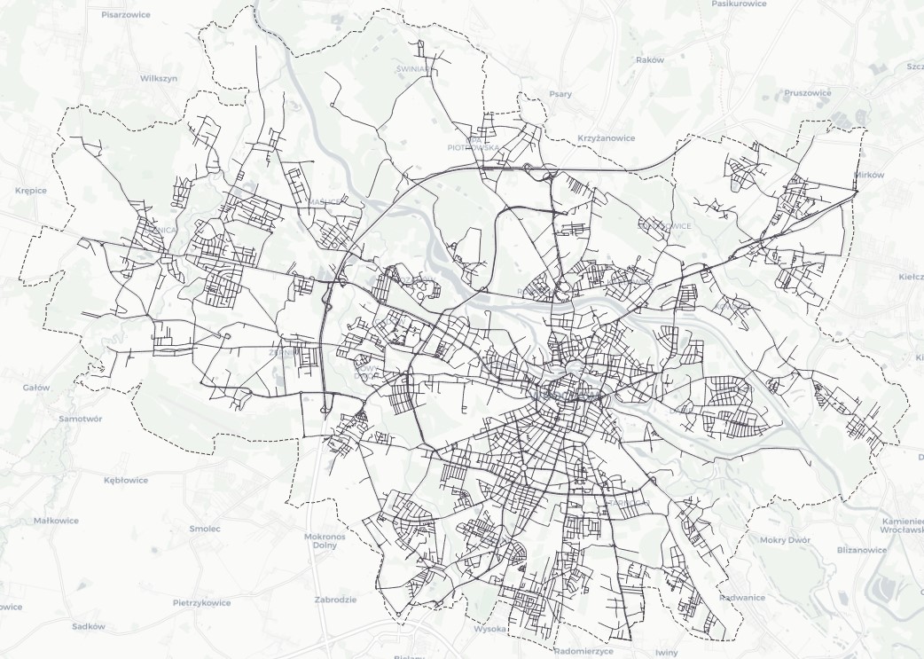
Figure 3. Road network

Figure 4. Obtained driveable road network for ’Wrocław, Poland’ query

3.1. Cities

As we concentrate mainly on urban areas, we assess the tags available in the OSM on a larger number of cities across the globe were downloaded than are actually used in the proposed solution. We downloaded $117$ cities on 2021-12-18 using the OSMnx library, which are shown in Figure 5.

Figure 5. Downloaded cities in Europe

The process of downloading the data uses geocoding, which converts the string query into geographic coordinates, and in the end, returns a polygon of a city. This process is visualized in Figure 6.

Figure 6. City selection process

Every city was manually checked to validate the quality of a query, and some cities were dropped from further analysis due to an incorrect polygon. The final distribution of $97$ selected cities.

3.2. Features

Every object in the OSM can contain multiple tags in the form of key-value pairs. As the OSM is a community-driven service with no strict enforcement on the data added (only guidelines exist), various keys and values may exist. It allows the service to be flexible, but at the same time, it lowers the quality of the data. Taginfo (OpenStreetMap Taginfo, [n.d.]) service was used to discover the available values of the features and their frequencies. It is a website that aggregates the tags and shows statistics about the values and tags used by the community. In addition, OSM Wiki (OpenStreetMap Wiki, [n.d.]) was utilized to understand the tags and possible values for the tags. Furthermore, a manual inspection of the data downloaded for $97$ selected cities across the globe was conducted. Based on these three approaches, the following keys were taken into consideration for the road segments of driveable road networks:

• oneway - whether the road is one-way,

• highway - rank of the road,

• surface - physical surface, structure, composition,

• maxspeed - maximum legal speed limit,

• lanes - number of traffic lanes,

• bridge - type of bridge that the way is on,

• junction - type of junction that the way forms itself,

• access - restrictions on the use,

• tunnel - type of an underground passage,

• width - actual width of a way.

Furthermore, every key has many values that need to be extracted, consolidated (e.g., brought to the same unit, rounded), and mapped. Then, the final set of features can be selected that will be treated as an input to the model. If the road segment contains a particular tag, the value is $1$; otherwise $0$. An example of features for one road segment is visible in Figure 7. Feature coverage varies between the cities. Figure 8 shows the key occurrence in the gathered data.

Figure 7. An example of features for one road segment

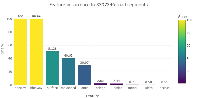
Figure 8. Feature keys occurrences in the obtained dataset of 97 selected cities

One can see that the most occurring features are oneway and highway, which are the essential information on road networks. No navigation system could use the road infrastructure data with these tags missing. Around 62% of roads are not one-way roads, and unsurprisingly, because the data is gathered solely from cities, the most common highway value is residential (around 58%).

The next common tags, that also relate to all of the roads, are surface (51%), maxspeed (40%) and lanes (30%). As we focus more on the highly urbanized areas in Europe, almost all of the streets are either asphalt or paved. The most common maxspeed values are $50$ and $30$, followed by $60$, which is also highly correlated to picking cities as the source of the data. Small lane values ($1$-$4$) are also popular in city road infrastructure.

A lot less roads contain bridge, junction, tunnel, or access tags, but these tags can be an important factor in differentiating the microregions that the roads belong to. The last tag, however not widely adopted, is width. It gives a better understanding of the physical form of the road. The most common widths are 5m and 6m, which for cities is highly correlated with the number of lanes, which is $2$. As an example, in Poland, the minimal width for a lane of a residential road is between 2,5m to 3,5m .

3.3. Microregions

H3 spatial index approach to partitioning cities into microregions was chosen. Based on the manual inspection of regions, the resolution value of 9 is believed to give the best trade-off between generalization and noise. Too tiny regions would mostly be able to capture single road segments, and as a consequence, the region embedding would be the same as a single road embedding. Too large regions, however, would contain roads of many different types and characteristics, leading to little regional variation. The H3 spatial index was chosen as separating the space into hexagons allows regions to an edge with all their neighbors, and the distance between the center of each region and the centers of each of its neighbors is the same.

Figure 9. Hex resolution comparison for the Grunwald Square and surroundings in Wrocław, Poland. The hexagon color reflects the resolution: black - 8, red - 9, blue - 10. Roads and intersections are shown in green and grey, respectively

4. Proposed solution

In this section, a method for obtaining vector representations of region-aggregated road infrastructure information is presented. It consists of three phases: partitioning the area into regions, feature aggregation, and representation learning. Finally, it is explained how the obtained vectors will be used to cluster regions into interpretable road infrastructure profiles. The methodology of the proposed solution is depicted in Figure 10.

Figure 10. Methodology of the proposed solution

4.1. Region embedding

In this section, the approach to generating region embeddings will be introduced. Firstly, the process of obtaining the representation of a particular road segment is presented, then the transformation from a road embedding space to a microregion latent space is described. As discussed in Section 3.3, H3 (Uber’s Hexagonal Hierarchical Spatial Index, [n.d.]) spatial index with resolution $9$ was used to partition the urban area into microregions. The utilization of a universal hierarchical spatial index provides portability across different cities and studies. It also enables combining the obtained representations for particular microregions. One can merge the embeddings to achieve more robust representations.

4.1.1. Autoencoder

To generate embeddings for road segments that are described by the features, the Autoencoder (Dong et al., 2018) neural network model was used. It is an unsupervised approach, at the core, high-dimensional unlabeled data need to be represented in a low-dimensional space, without the need of labeling that data.

Figure 11. Architecture of the used Autoencoder method

The Autoencoder consists of two parts - an encoder and a decoder. The former’s responsibility is to reduce the dimensionality of the input data $X$, and in the end, it outputs the lower-dimensionality version - an embedding $h$. The latter is to reconstruct the input $X^{\prime}$ from the obtained embedding. The architecture of the Autoencoder proposed in this paper is depicted in 11 and also described below.

Encoder:

• Input layer - 88 features,

• Linear layer with ReLU - 64 dimensions,

• Embedding layer - 30 dimensions.

Decoder:

• Embedding layer - 30 dimensions,

• Linear layer with ReLU - 64 dimensions,

• Linear layer - 88 dimensions.

The Autoencoder uses a backpropagation algorithm (Linnainmaa, 1976). The training is based on minimizing the reconstruction loss. There are several loss functions suited for different tasks: Mean Squared Error (MSE) or Binary Cross Entropy (BCE). Using BCE would be a natural approach to handling binary features of the road segments, however, the obtained embeddings proved to be sub-par to the ones generated with MSE. In the end, the loss was chosen to be the Mean Squared Error, which for the input X is defined as follows:

(1) $$L=MSE=\frac{1}{N}\sum_{n=1}^{N}(X_{n}-X^{\prime}_{n}).$$

4.1.2. Roads aggregation

To generate the region representations, the road segments within must be aggregated. All roads that intersect with a hexagon, count to a particular microregion. A visual representation for different cases of aggregation is shown in Figure 12.

Figure 12. Road features aggregation into hexagons. Road $1$ is aggregated to hexagon $A$, road $2$ is aggregated to hexagons $A$ and $B$, road $3$ is aggregated to hexagons $A$, $B$, and $C$

One can choose the aggregation function of the road embeddings. The embeddings that belong to a particular microregion are averaged, which results in one representation for the region in the same latent space as the road segment embeddings. As the co-occurrence of the features in the road segments is essential, aggregation cannot be performed before the road segment embedding process. Simply counting the tags that a region has, followed by embedding that region, will lose information about the characteristics of particular roads. The final profile of the region would not represent the contained roads accurately.

4.2. Similarity detection

Having the urban space partitioned into microregions, and the representations in the latent space of such regions, one can detect similarities between them. Using the knowledge gathered during the review of the literature in Section 2 multiple approaches to visualizing and defining the obtained latent space will be presented.

4.2.1. Agglomerative Clustering

One of the approaches to detect similarities between regions is to find the groups that the underlying data naturally forms. Based on that, the analyses can be done for particular groups instead of single instances, which can provide a more insightful comparison. In addition, obtaining the hierarchy of groups may further aid the process of determining the region typology. For that purpose, the hierarchical clustering method was used - Agglomerative Clustering (Patel et al., 2015). It is based on the bottom-up approach, where at the beginning each instance is in its own cluster, and the clusters are merged successively. The pairs which minimize the linkage criterion (difference between the sets) are merged. The Ward (Jr., 1963) linkage criterion was used, which focuses on minimizing the variance of the groups. To compute the linkage, a distance metric is needed, and for that, the euclidean distance was used. Looking at the feature distribution in the clusters, one can identify the characteristics of particular groups. Considering also multiple levels of hierarchical groups, a region typology based on road infrastructure in cities will be established.

4.2.2. Latent space analysis

To analyze the obtained latent space, dimensionality reduction techniques will be used to provide embeddings suited for visualizations. Principal Component Analysis (PCA) (F.R.S., 1901) will aid in showing the diversification of regions in cities. It will lower down the dimensionality of the embeddings to $3$, and later convert the obtained values to the RGB color space. Furthermore, t-Distributed Stochastic Neighbor Embedding (t-SNE) (van der Maaten and Hinton, 2008) will enable looking into the embedding space in $2$ dimensions, to see how the space is laid out. Additionally, operations on the obtained embeddings will be performed (similar to (Gittens et al., 2017)) - adding and subtracting - to find if the semantic meaning of the real-world objects is preserved.

5. Experiments

In this section, we present the experimental results. First, the setting for the model training will be described. Then the hierarchical clustering results will be shown, followed by the defined region typology. Finally, the visualizations of the obtained latent space will be presented and the operations will be performed.

5.1. Setting

Training and testing the Autoencoder neural network proposed in Subsection 4.1.1 was performed on a subset of data described in Section 3. The data consists solely of $13$ Polish cities. It contains $191868$ road segments and $22991$ H3 microregions, that contain at least one road. Other hexagons are not considered. Similarity detection and latent space visualizations will also be performed on the same dataset, however, the clustering results will only be shown for $6$ selected cities.

The network architecture was defined in Subsection 4.1.1. The proposed pipeline, however, needs additional hyperparameters defined. The values are as follows:

• optimizer - Adam with learning rate $0.001$,

• batch size - $200$,

• epochs - $50$,

• test dataset ratio - $0.2$,

• t-SNE perplexity - $100$.

5.2. Similarity detection

This section will provide the results for multiple levels of hierarchical clustering. At the end, the region typology will be proposed.

5.2.1. Hierarchical clustering

Hierarchical clustering provides a cluster tree that represents the successive splits of groups. Such visualization is called dendrogram and is shown in Figure 13. It can give an overview of how the partitioning process will look like. As stated in Section 4, the Agglomerative clustering method was used in generating the data splits.

Figure 13. Dendrogram for the dataset

The rest of this section will be organized as follows - for every division a description will be provided, accompanied with visualizations of clustered microregions for selected Polish cities. Additionally, a difference between the two divided clusters will be presented. A cluster is called new if the overall number of microregions in this cluster is fewer than in the other old cluster. The difference for a particular tag between the new and old groups is simply the difference in the share of this tag in the corresponding feature.

5.2.2. Region typology

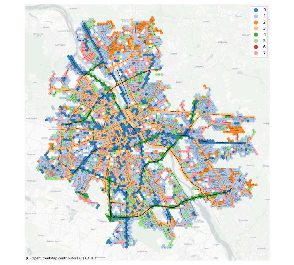
(c) Warszawa

(d) Wrocław

Figure 17. Microregion clustering results ($8$ clusters) for selected Polish cities

This section summarizes the results of the hierarchical clustering experiments carried out on 13 Polish cities. The groupings of the microregions for different splits were discussed and based on these results, the region typology will be proposed. The final number of clusters was determined to be $8$, as further splits do not provide meaningful information and oftentimes are a product of artifacts in the data (e.g., incomplete tag information for road segments). The obtained embeddings are capable of generating a diversified profile of microregions across multiple cities. The grouped zones for selected urban areas are shown in Figure 17, and the final profiles of microregions can be described as follows:

• $0$ - high-capacity regions containing arterial roads,

• $1$ - residential, paved regions with good quality of road infrastructure,

• $2$ - residential, unpaved regions with low quality of road infrastructure,

• $3$ - regions complementing main road network,

• $4$ - high-capacity, high-speed regions and bypasses,

• $5$ - estate regions and connectors,

• $6$ - motorways,

• $7$ - traffic collectors and connectors.

The obtained region typology properly diversifies the city regions into multiple functionally meaningful groups in terms of road infrastructure. The final share of features across all clusters is depicted in Figure 18. The proposed solution generates satisfactory results and enables automatic discovery of the city structure. Furthermore, it validates the quality of the obtained latent space and the used methodology.

The blue cluster 0 regional profile was still unclear and contained a lot of different types of main roads in cities. The $8$ cluster split happened exactly on that one. Let’s start with the Figure 14. The new light red cluster 7 regions are made up of tertiary two-way roads, and as a consequence, the other cluster contains primary one-way road infrastructure. As a result, the light red cluster 7 profile is mostly described by collector roads in the city. Comparing it to the maps (Figure 17), one can see that these regions’ purpose is to connect areas and provide an infrastructure responsible for accessing the main arterial roads within a city. Take Wrocław for an instance. The entire right side of a city depends on the new cluster traffic-wise, as well as on light orange cluster 3. Light red cluster 7 regions grant residential areas (light blue) access to the main part of the road network. Further splits introduce noise, and meaningful diversification of the microregions becomes difficult. Often, the partitioning results from artifacts in the data (e.g., missing tags).

Figure 14. Cluster difference between $7$ and $0$ for $8$ clusters

5.3. Latent space analysis

To further validate the quality of the representations, the obtained space can be analyzed. As a reminder, the road segments containing OSM tags were embedded and then aggregated (averaged) to their corresponding microregions. The resulting regional vectors are in the same space as the road embeddings. t-SNE was used to visualize the microregion representations in $2$ dimensions. Additionally, the grouping from the previous section was utilized. The result is depicted in Figure 15.

Figure 15. Latent space visualization using t-SNE and colour-coded in $8$ clusters

One can see that the clusters are rather separated. Green cluster 4 and red cluster 6 are both represented by high-capacity, high-speed roads, but the distinction between motorways and trunk roads is apparent. Light orange cluster 3 regions are also separated from others as the group focuses mostly on secondary roads. The big initial blue cluster 0 got divided to the point that eventual further splits could contain a lot of noise. Moving to the second initial light blue cluster 1, which contained paved residential areas - it did not separate that well. Two large concentrations of regions are visible around $(20,-60)$ and $(-40,30)$. These could be separated in further splits. The rest of this cluster is spread, and that could mean that the functional profile of this group can be fuzzy. The orange cluster 2 also contains residential roads but focuses on the unpaved aspect of the road’s surface. The light green cluster 5 has one highly concentrated zone and four other smaller zones. Probably the difference is in estate areas and connectors, and the division would happen in further splits. The last cluster, light red cluster 7, containing mainly distributor roads is situated near blue cluster 0, which contains arterial roads. It makes sense in terms of the functional purposes of the microregions.

5.3.1. Semantic arithmetics

The last experiment will perform arithmetic operations on the obtained embedding space to validate if the semantic meaning of the real-world objects is preserved. We show how addition between two embedded microregions exhibits semantic phenomena.

(a) High-traffic region containing a bridge in Wrocław, Poland.

(b) Residential region in Wrocław, Poland.

(c) Residential area next to high-traffic roads in Poznań, Poland.

Figure 16. Addition in the obtained embedding space (Blue + Green = Red)

First, the addition of two vectors is performed, conditioned on the resulting embedding being in Poznań. Two microregions from Wrocław are selected, which are distinct in their nature and serve one purpose in the city road infrastructure. These two regions are high-traffic (with a bridge) and residential regions, respectively. The sum of the embeddings yields a functionally merged region, which is a residential region adjacent to high-traffic roads. This process is shown in Figure 16. Looking at the feature profiles of the microregions, one can see that share-wise the resulting zone is an imperfect merger of the summands. However, the most important tag that is not taken into account is bridge, which is at the core of the second microregion.

6. Conclusions

We propose a method for the unsupervised embedding of microregions using road infrastructure information and use the obtained latent space to conduct similarity detection, and as a result, define a typology of city regions. To accomplish the stated goals, several subtasks were specified and completed.

Using the proposed method, the road segments for $13$ Polish cities were embedded, which later were aggregated to their corresponding microregions, eventually creating their representations. Then, similarity detection was performed on the obtained latent space using Agglomerative Clustering. This resulted in the grouping of the different numbers of clusters. Each such division was later discussed and analyzed, which in the end resulted in the high-level definition of region typology based on road infrastructure information. Finally, the obtained latent space was analyzed, and arithmetic operations such as addition and subtraction of the embedding vectors were performed. Carrying out the experiments proved that the obtained representations carry meaningful information and the semantic meaning of the real-world objects is preserved.

Although the proposed solution seems simple, the final results prove that it could capture the characteristics of the road network. Furthermore, it provided diversified enough urban zone representations upon which the region typology could be defined. Additionally, an automatic way of discovering the city’s road structure was identified.

7. Future works

We believe that the proposed methodology provides the backbone for further development in the area of geospatial data, and more specifically, in the region embedding using road infrastructure information. Based on the input of this thesis, some further improvements can be identified, such as:

• graph aspect - road infrastructure is intrinsical of graph nature. One could use methods that use this type of data fully. Previous works experimented with this approach but lacked in using spatial indexes,

• roads position and orientation - this thesis does not consider these aspects. Enriching the model with such information could further improve the model,

• model change - the autoencoder used in this thesis is a basic approach. One can try utilizing more advanced solutions - VAE (Kingma and Welling, 2014) or beta-VAE (Higgins et al., 2017) - or try Skip-Gram (Mikolov et al., 2013) approach to geospatial data, as used in (Woźniak and Szymański, 2021),

• downstream tasks - evaluating method quantitatively on predictive tasks would enable comparing the obtained embeddings to other methods,

• intersections - data available in the intersections could be incorporated into the method,

• network types - this thesis was based on driveable road networks. One could try to apply the methodology to other types of road networks (bicycle road infrastructure, railways, etc.),

• data augmentation - publicly available open-data sources such as OpenStreetMap are not complete and a significant portion of the data is missing. One could try to impute the tags using other present features, and national or domestic laws,

• region aggregation - in this thesis, the road embeddings were equally aggregated into the corresponding regions. Weighting the road segments, e.g., by the road length in this region, could be beneficial,

• data range - incorporating more cities around the globe or even adding areas outside the cities could result in a more robust method.

Appendix A Histograms and typology maps

(a) Poznań

(b) Trójmiasto (Gdańsk, Gdynia, Sopot)

(a) Access

(b) Bridge

(c) Highway

(d) Junction

(e) Lanes

(f) Maxspeed

(g) Oneway

(h) Surface

(i) Tunnel

(j) Width

Figure 18. Features’ shares in final groups

References

- (1)
- Boeing (2017) Geoff Boeing. 2017. OSMnx: New methods for acquiring, constructing, analyzing, and visualizing complex street networks. Computers, Environment and Urban Systems 65 (2017), 126–139. https://doi.org/10.1016/j.compenvurbsys.2017.05.004
- Dong et al. (2018) Ganggang Dong, Guisheng Liao, Hongwei Liu, and Gangyao Kuang. 2018. A Review of the Autoencoder and Its Variants: A Comparative Perspective from Target Recognition in Synthetic-Aperture Radar Images. IEEE Geoscience and Remote Sensing Magazine 6, 3 (2018), 44–68. https://doi.org/10.1109/MGRS.2018.2853555
- Du et al. (2018) Jiahong Du, Yujun Chen, Yue Wang, and Juhua Pu. 2018. Zone2Vec: Distributed Representation Learning of Urban Zones. 2018 24th International Conference on Pattern Recognition (ICPR) (2018), 880–885.
- F.R.S. (1901) Karl Pearson F.R.S. 1901. LIII. On lines and planes of closest fit to systems of points in space. The London, Edinburgh, and Dublin Philosophical Magazine and Journal of Science 2, 11 (1901), 559–572. https://doi.org/10.1080/14786440109462720
- Gittens et al. (2017) Alex Gittens, Dimitris Achlioptas, and Michael W. Mahoney. 2017. Skip-Gram - Zipf + Uniform = Vector Additivity. In Proceedings of the 55th Annual Meeting of the Association for Computational Linguistics (Volume 1: Long Papers). Association for Computational Linguistics, Vancouver, Canada, 69–76. https://doi.org/10.18653/v1/P17-1007
- Grover and Leskovec (2016) Aditya Grover and Jure Leskovec. 2016. Node2vec: Scalable Feature Learning for Networks. In Proceedings of the 22nd ACM SIGKDD International Conference on Knowledge Discovery and Data Mining (San Francisco, California, USA) (KDD ’16). Association for Computing Machinery, New York, NY, USA, 855–864. https://doi.org/10.1145/2939672.2939754
- Higgins et al. (2017) Irina Higgins, Loïc Matthey, Arka Pal, Christopher P. Burgess, Xavier Glorot, Matthew M. Botvinick, Shakir Mohamed, and Alexander Lerchner. 2017. beta-VAE: Learning Basic Visual Concepts with a Constrained Variational Framework. In 5th International Conference on Learning Representations, ICLR 2017, Toulon, France, April 24-26, 2017, Conference Track Proceedings. OpenReview.net. https://openreview.net/forum?id=Sy2fzU9gl
- Jenkins et al. (2019) Porter Jenkins, Ahmad Farag, Suhang Wang, and Zhenhui Li. 2019. Unsupervised Representation Learning of Spatial Data via Multimodal Embedding. In Proceedings of the 28th ACM International Conference on Information and Knowledge Management (Beijing, China) (CIKM ’19). Association for Computing Machinery, New York, NY, USA, 1993–2002. https://doi.org/10.1145/3357384.3358001
- Jr. (1963) Joe H. Ward Jr. 1963. Hierarchical Grouping to Optimize an Objective Function. J. Amer. Statist. Assoc. 58, 301 (1963), 236–244. https://doi.org/10.1080/01621459.1963.10500845 arXiv:https://www.tandfonline.com/doi/pdf/10.1080/01621459.1963.10500845
- Kempinska and Murcio (2019) Kira Kempinska and Roberto Murcio. 2019. Modelling urban networks using Variational Autoencoders. Applied Network Science 4 (2019), 1–11.
- Kingma and Welling (2014) Diederik P Kingma and Max Welling. 2014. Auto-Encoding Variational Bayes. arXiv:1312.6114 [stat.ML]
- Kipf and Welling (2017) Thomas N. Kipf and Max Welling. 2017. Semi-Supervised Classification with Graph Convolutional Networks. arXiv:1609.02907 [cs.LG]
- Linnainmaa (1976) Seppo Linnainmaa. 1976. Taylor expansion of the accumulated rounding error. BIT Numerical Mathematics 16 (1976), 146–160.
- Mikolov et al. (2013) Tomas Mikolov, Kai Chen, G.s Corrado, and Jeffrey Dean. 2013. Efficient Estimation of Word Representations in Vector Space. Proceedings of Workshop at ICLR 2013 (01 2013).
- OpenStreetMap ([n.d.]) OpenStreetMap [n.d.]. OpenStreetMap. https://www.openstreetmap.org/about. Accessed: 2022-01-14.
- OpenStreetMap Taginfo ([n.d.]) OpenStreetMap Taginfo [n.d.]. OpenStreetMap Taginfo. https://taginfo.openstreetmap.org/. Accessed: 2022-01-22.
- OpenStreetMap Wiki ([n.d.]) OpenStreetMap Wiki [n.d.]. OpenStreetMap Wiki. https://wiki.openstreetmap.org/wiki/Main_Page. Accessed: 2022-01-24.
- Patel et al. (2015) Sakshi Patel, Shivani Sihmar, and Aman Jatain. 2015. A study of hierarchical clustering algorithms. In 2015 2nd International Conference on Computing for Sustainable Global Development (INDIACom). 537–541.
- Spruyt, Vincent (2018) Spruyt, Vincent. 2018. Loc2Vec: Learning location embeddings with triplet-loss networks. https://sentiance.com/2018/05/03/loc2vec-learning-location-embeddings-w-triplet-loss-networks/. Accessed: 2022-01-16.
- Tobler (1970) W. R. Tobler. 1970. A Computer Movie Simulating Urban Growth in the Detroit Region. Economic Geography 46 (1970), 234. https://doi.org/10.2307/143141
- Uber’s Hexagonal Hierarchical Spatial Index ([n.d.]) Uber’s Hexagonal Hierarchical Spatial Index [n.d.]. Uber’s Hexagonal Hierarchical Spatial Index. https://eng.uber.com/h3/. Accessed: 2022-01-14.
- van der Maaten and Hinton (2008) Laurens van der Maaten and Geoffrey Hinton. 2008. Visualizing Data using t-SNE. Journal of Machine Learning Research 9, 86 (2008), 2579–2605. http://jmlr.org/papers/v9/vandermaaten08a.html
- Veličković et al. (2018) Petar Veličković, Guillem Cucurull, Arantxa Casanova, Adriana Romero, Pietro Liò, and Yoshua Bengio. 2018. Graph Attention Networks. arXiv:1710.10903 [stat.ML]
- Wang et al. (2019) Meng-xiang Wang, Wang-Chien Lee, Tao-yang Fu, and Ge Yu. 2019. Learning Embeddings of Intersections on Road Networks. In Proceedings of the 27th ACM SIGSPATIAL International Conference on Advances in Geographic Information Systems (Chicago, IL, USA) (SIGSPATIAL ’19). Association for Computing Machinery, New York, NY, USA, 309–318. https://doi.org/10.1145/3347146.3359075
- Wang et al. (2020) Meng-Xiang Wang, Wang-Chien Lee, Tao-Yang Fu, and Ge Yu. 2020. On Representation Learning for Road Networks. ACM Trans. Intell. Syst. Technol. 12, 1, Article 11 (dec 2020), 27 pages. https://doi.org/10.1145/3424346
- Woźniak and Szymański (2021) Szymon Woźniak and Piotr Szymański. 2021. Hex2vec: Context-Aware Embedding H3 Hexagons with OpenStreetMap Tags. Association for Computing Machinery, New York, NY, USA, 61–71. https://doi.org/10.1145/3486635.3491076
- Wu et al. (2020) Ning Wu, Xin Wayne Zhao, Jingyuan Wang, and Dayan Pan. 2020. Learning Effective Road Network Representation with Hierarchical Graph Neural Networks. Association for Computing Machinery, New York, NY, USA, 6–14. https://doi.org/10.1145/3394486.3403043
- Yao et al. (2018) Zijun Yao, Yanjie Fu, Bin Liu, Wangsu Hu, and Hui Xiong. 2018. Representing Urban Functions through Zone Embedding with Human Mobility Patterns. In Proceedings of the Twenty-Seventh International Joint Conference on Artificial Intelligence, IJCAI-18. International Joint Conferences on Artificial Intelligence Organization, 3919–3925. https://doi.org/10.24963/ijcai.2018/545