Bootstrapped Edge Count Tests for Nonparametric Two-Sample Inference Under Heterogeneity

Abstract

Nonparametric two-sample testing is a classical problem in inferential statistics. While modern two-sample tests, such as the edge count test and its variants, can handle multivariate and non-Euclidean data, contemporary gargantuan datasets often exhibit heterogeneity due to the presence of latent subpopulations. Direct application of these tests, without regulating for such heterogeneity, may lead to incorrect statistical decisions. We develop a new nonparametric testing procedure that accurately detects differences between the two samples in the presence of unknown heterogeneity in the data generation process. Our framework handles this latent heterogeneity through a composite null that entertains the possibility that the two samples arise from a mixture distribution with identical component distributions but with possibly different mixing weights. In this regime, we study the asymptotic behavior of weighted edge count test statistic and show that it can be effectively re-calibrated to detect arbitrary deviations from the composite null. For practical implementation we propose a Bootstrapped Weighted Edge Count test which involves a bootstrap-based calibration procedure that can be easily implemented across a wide range of heterogeneous regimes. A comprehensive simulation study and an application to detecting aberrant user behaviors in online games demonstrates the excellent non-asymptotic performance of the proposed test.

Keywords: composite hypothesis testing; consumer behavior analysis; heterogeneity; two-sample tests.

1 Introduction

Nonparametric two-sample testing is a classical problem in inferential statistics. The use of these tests is pervasive across disciplines, such as medicine (Farris and Schopflocher, 1999), consumer research (Folkes et al., 1987), remote sensing (Conradsen et al., 2003) and public policy (Rothman et al., 2006), where detecting distributional differences between the two samples is germane to the ongoing scientific analysis. Nonparametric two-sample tests like the Kolmogorov-Smirnov test, the Wilcoxon rank-sum test, and the Wald-Wolfowitz runs test are extremely popular tools for analyzing univariate data. Multivariate versions of these tests have their origins in the randomization tests of Chung and Fraser (1958) and in the generalized Kolmogorov-Smirnov test of Bickel (1969). Friedman and Rafsky (1979) proposed the first computationally efficient nonparametric two-sample test, the edge count test, for high-dimensional data. Modern versions of the edge count test, such as the weighted and generalized edge count test (Chen and Friedman, 2017; Chen et al., 2018), can handle multivariate data, and can be applied to any data types as long as an informative similarity measure between the data points can be defined. Besides the edge count tests, several tests based on nearest-neighbor distances (Henze, 1984; Schilling, 1986; Chen et al., 2013; Hall and Tajvidi, 2002; Banerjee et al., 2020) and matchings (Rosenbaum, 2005; Mukherjee et al., 2022) have been proposed over the years, and used in variety of applications, such as covariate balancing (Heller et al., 2010a, b), change point detection (Chen and Zhang, 2015; Shi et al., 2017), gene-set analysis (Rahmatallah et al., 2012), microbiome data (Callahan et al., 2016; Holmes and Huber, 2018; Fukuyama, 2020), among others.

Bhattacharya (2019) propose a general framework to study the asymptotic properties of these graph based tests. In addition to the graph based tests, other popular two-sample tests include the energy distance test of Székely (2003) and Székely and Rizzo (2004) (see also Baringhaus and Franz (2004); Aslan and Zech (2005); Székely and Rizzo (2013)), and kernel tests based on the maximum mean discrepancy (see Gretton et al. (2007); Chwialkowski et al. (2015); Ramdas et al. (2015, 2017) and the references therein). Recently, several authors have proposed distribution-free two-sample tests using optimal transport based multivariate ranks (see Deb and Sen (2021); Ghosal and Sen (2019); Shi et al. (2020a), and Shi et al. (2020b) and the references therein).

While there exists a vast literature on nonparametric two-sample tests, their performance in scenarios where the two samples might contain different heterogeneous structures have not been well-explored before. However, in a host of contemporary data analysis problems (See Ch. 3 of Holmes and Huber (2018), Rossi et al. (2012)) there is a need to conduct inference in presence of unknown heterogeneity in the data generation process. This is particularly important when there are latent subpopulations in the two populations from which the samples were extracted. Detecting distributional differences across the two samples is challenging in the presence of such heterogeneity because the two samples may differ with respect to the rates with which they arise from the underlying subpopulations. In these settings, direct application of existing two-sample tests, without regulating for the latent heterogeneity in the samples, may lead to incorrect statistical decisions and scientific consequences. In this article, we develop a new nonparametric testing procedure that can accurately detect if there are differences between the two samples in the presence of latent heterogeneity in the data generation process. We next present two contemporary data examples to motivate the two-sample testing problem under heterogeneity and discuss how existing tests may lead to incorrect decisions in the presence of heterogeneity.

1.1 Motivating examples for testing under heterogeneity

Example 1: Detecting shift in consumer sentiment and spending pattern – Detecting shifts in consumer sentiment and their spending pattern in response to exogenous economic shocks, such as a pandemic, war or supply chain constraints, is important from the perspective of public policy and businesses operations across different sectors (Agarwal et al., 2019; Crouzet et al., 2019; Bruun, 2021; Bartik et al., 2020). Evidence of such changes in spending pattern is used to make policy decisions on the allocation of future resources to tackle the shifting landscape of consumer demand (Balis, 2021; Liguori and Pittz, 2020; Akpan et al., 2022). Data privacy rules, however, often forbid using personally identifiable information, such as individual consumer demographics and spending patterns over time, thus ruling out the possibility of acquiring a rich consumer level panel data and utilizing sophisticated tools from causal inference to detect changes in spending patterns in response to the event of interest. A two-sample statistical test of hypothesis is often conducted to determine whether the spending pattern of a sample of consumers before the event of interest is significantly different from the spending pattern of an independent sample of consumers during or after the event of interest. Despite being much less powerful than tests based on comprehensive longitudinal data, the two-sample tests have the advantage of being substantially more privacy-preserving as these non-intrusive tests only need two independent vectors of observations and thus can be implemented across a wide range of contemporary applications. However, there are two main challenges for devising a test of hypothesis that can correctly detect such differences in the spending pattern between these two independent samples:

1. The two samples may exhibit sample size imbalances which presents a challenging setting for nonparametric two-sample testing on multivariate data (Chen et al., 2018).

2. The consumer base may consist of several heterogeneous subpopulations with respect to their consumption behavior. In business and economic modeling it is now commonplace to model such consumption behavior as a mixture of several distinct consumption patterns (Fahey et al., 2007; Labeeuw and Deconinck, 2013).

Due to an exogenous shock we can have one of the following three situations regarding the behavior of consumers after the shock:

1. Consumer behavior does not change and maintains the pre-shock levels.

2. Consumption behavior changes but there are no new consumption patterns. The change in the consumption distribution is due to changes in the proportions of existing modes of consumption. This is the case where there is switching between the different consumption modes but no new consumption patterns evolve due to the external shock.

3. Consumption behavior changes and there are new consumption patterns that were previously non-existent.

In this paper, we concentrate on the detection of the third case, Case III, where new consumption patterns emerge post-shock. Accurate and timely identification of Case III is important for it allows researchers to understand if deviant forms of consumption (Koskenniemi, 2021) arise after a critical event, which can then be subsequently studied and analyzed with higher granularity data. Statistically, the main challenge here lies in correctly detecting Case III while not misidentifying Cases I and II as type I error. Two-sample testing procedures in the existing literature (discussed at the beginning of Section 1) are designed to distinguish between Cases I and II. We will show that without modifications their direct usage do not produce correct inference for this exercise.

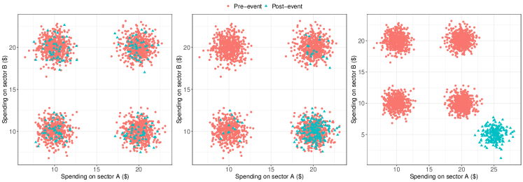
Figure 1: Testing shift in consumer spending pattern due to external economic shock. Green triangles represent a sample of consumers post-event, while the red dots represent an independent sample of consumers pre-event. The pre-event sample exhibits four distinct subpopulations. Left– consumption pattern of post-event consumers originate from these four subpopulations with equal probabilities. Center– majority of the post-event consumers arise from one of the four subpopulations without a shift in the levels of their consumption for that subpopulation. Right– post-event consumers originate from a new subpopulation that exhibits a change in the levels of consumption after the shock. The simulation scheme for these plots is described in Section B of the supplement.

We further elucidate this problem with the help of a simple simulation example. Consider a bivariate consumption problem with consumption on sector A denoted by $X_{1}$ and on sector B by $X_{2}$. We have bivariate observations $(X_{1},X_{2})$ for two random samples of customers before and after the shock (event). In Figure 1, the red dots represent the sample of consumers pre-event, while the green triangles represent an independent sample of consumers post-event. The three plots in Figure 1 present the distribution of spending pattern with respect to $(X_{1},X_{2})$ and reveals that the pre-event sample exhibits four distinct subpopulations. The leftmost panel represents the setting where the consumption pattern of post-event consumers originate from these four subpopulations with equal probabilities. The center panel presents the setting of Case II where a majority of the post-event consumers arise from one of the four subpopulations without a shift in the levels of their consumption for that subpopulation. This represents normal consumption with only the proportional representation of the latent states of normal consumption being changed. The rightmost panel, on the other hand, reveals that the post-event consumers originate from a new subpopulation that exhibits a change in the levels of consumption after the event (Case III).

Distinction between the two settings presented in the center (Case II) and right (Case III) panels of Figure 1 is critical for policy makers and marketeers. In this paper, we develop a consistent two-sample testing framework that can detect Case III from Cases I and II in the presence of sample size imbalance as well as heterogeneity. We next discuss another motivating example regarding consumption of digital entertainment, which will be further pursued in Section 5.

Example 2: Detecting differences in player behavior in online games – Online gaming is an important component of modern recreational and socialization media (Banerjee et al., 2022). For monetization of these digital products, managers often have to deliver personalized promotions to users based on their product usage. Additionally, through promotional intervention the portal needs to regulate addiction, violence and other deviant consumption patterns (Hull et al., 2014) than can cause long term societal harms. As it is difficult to manually track every game, the portals use automated decision rules to monitor the game sessions and rely on features extracted at regular intervals of time, such as hourly or half-hourly, to constantly check for deviant consumption within each game session. When evidence of preponderance of deviant consumption is available, managerial interventions are made.

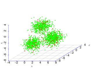
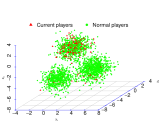
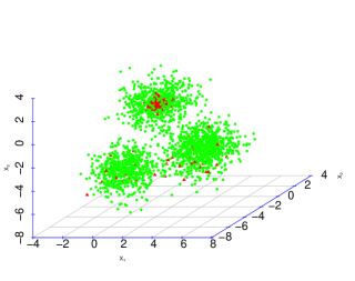
Figure 2: Differences in playing behavior in online video games. Red triangles represent the sample of current players, while the green dots are the sample of normal players from historical logs. The green sample exhibits three distinct subpopulations. Left– Case I: Current sample originates from three subpopulations present in the green sample with equal probabilities. Center– Case II: most members in the current sample originate from only one of the three subpopulations. Right– Case III: current sample originates from one of the three subpopulations but exhibits a different scale. The simulation scheme for these plots is described in Section B of the supplement.

Statistically, the problem here again reduces to the correct detection of scenarios pertaining to Case III described in Figure 1 above. To see this, note that based on historical data a multivariate sample of gaming features from players corresponding to normal gaming characteristics is available. The size of such a sample is huge as it is based on historical logs. The goal is to compare the instantaneous gaming features of a subset (gated by region, age, etc) of currently logged-on players with respect to this sample. The sample size of this subset of players is much smaller than the benchmark normal gaming consumption sample and so, we encounter the issue of sample size imbalance. Additionally, while comparing these two samples we are interested in detecting if there is a sub-population of players with deviant gaming characteristics which would need regulating promotional incentives related to purchase of gaming artifacts. This again corresponds to different Case III scenarios described above. Even without any instance of deviant usage, instantaneous gaming characteristics greatly change over time-of-day, for instance early morning players and evening players have varying characteristics. This corresponds to scenarios in Case II. Thus, the goal will be to detect Case III scenarios while allowing the possibility for scenarios from Cases I and II. We illustrate this through a simulation example in Figure 2.

Consider observing $d=3$ dimensional characteristics, $X_{1},X_{2}$ and $X_{3}$ of playing behavior. The green dots in Figure 2 represent the sample of normal players from historical records. It exhibits three distinct subpopulations of equal sizes. The red triangles represent the sample of players from a current session. The leftmost panel depicts a setting where the current sample originates from these three subpopulations with equal probabilities (an instance of Case I). The center panel presents the setting where a majority of the players in the current sample are from one of the three subpopulations (an instance of Case II), and the rightmost panel reveals an instance of Case III where there is a new sub-population represented by red triangles that was non-existent in normal players. Note that, unlike Figure 1 here the deviant sub-population differs from one of the three subpopulations of normal players only in scale and not in locations. Detecting this case is more difficult than Figure 1 and we present a detailed analysis in Section 4. In Section 5 we develop this example and apply our proposed hypothesis testing method to detect addictive behaviors in a real-world gaming dataset.

1.2 Two-sample testing under heterogeneity and our contributions

Existing nonparametric two-sample tests cannot distinguish between the scenarios presented in the center and right panels of Figures 1 and 2. For instance, the edge count test (Friedman and Rafsky, 1979), the weighted edge count test (Chen et al., 2018) and the generalized edge count test (Chen and Friedman, 2017) reject the null hypothesis of equality of the two distributions for both Cases II and III in Figures 1 and 2 (see tables 7 and 8 in Section B of the supplement for more details). This is not surprising because these nonparametric two-sample tests are designed to test the simple null hypothesis of equality of the two distributions (Case II vs Case I) and directly using them, without any modification, to detect Case III scenarios from Case II can be misleading. To resolve this conundrum, we develop a hypothesis testing framework based on an appropriately constructed composite null hypothesis (Equations (5)–(7)). Under this composite null hypothesis, we study the properties of the Weighted Edge Count (WEC) test statistic of Chen et al. (2018) and show that it can be re-calibrated to produce an asymptotically consistent two-sample test. For finite sample applications, we propose a bootstrap-based calibration procedure for the WEC test statistic that allows it to consistently and efficiently detect differences between the two samples under subpopulation level heterogeneity. The ensuing discussion summarizes our key contributions.

• We study the asymptotic properties of the WEC statistic for the heterogeneous two-sample problem (Section 2). Specifically, we show how one can choose a cut-off that renders the WEC statistic asymptotically powerful for detecting any distribution that significantly deviates from the composite null hypothesis (see Equation (7)), which encompasses the possibility that the two samples arise from the same mixture distribution but with possibly different mixing weights (see Proposition 1). This is in contrast to the TRUH test in Banerjee et al. (2020) which can only detect deviations in location under the concerned composite null hypothesis. This is because, unlike the TRUH statistic which compares the nearest neighbor distances between the two-samples, the WEC statistic is based on the number of within sample edges in a similarity graph of the pooled sample. The combinatorial (count-type) nature of the WEC statistic renders it asymptotically distribution-free under the simple (homogeneous) null, that is, the distribution of the test statistic does not depend on the null distribution of the data. Moreover, the WEC statistic estimates the well-known Henze-Penrose divergence (see Equation (9) for the definition) and, consequently, can detect arbitrary differences between two distributions under the homogeneous null. We leverage these properties to obtain a cut-off for the WEC statistic that can detect deviations from the heterogeneous (composite) null, beyond location problems.

• For non-asymptotic usage, we develop a novel bootstrap-based calibration procedure for the weighted edge count test statistic (Algorithm 1 in Section 3) and use it to test the composite null hypothesis that the two samples arise from the same mixture distribution but with possibly different mixing weights (Equations (5)–(7)). Under sample size imbalance, our calibration procedure first explores the larger sample for heterogeneous subgroups. Then it generates an ensemble of mixing weights for the different subgroups and subsequently constructs a collection of surrogate two-samples under the composite null hypothesis. The WEC test statistic is computed for each such surrogate two-samples and the ensemble of these WEC test statistics is then used to determine the level $\alpha$ cutoff for testing the composite null hypothesis (Equation (7)).

• Our numerical experiments (Section 4) reveal that across a wide range of simulation settings, the proposed bootstrap calibration procedure results in a conservative level $\alpha$ cutoff for the WEC test statistic for consistent nonparametric two sample testing involving the composite null hypothesis of Equation (7). This is in contrast to existing nonparametric two-sample tests that may lead to incorrect inference in this regime. Furthermore, our empirical evidence suggests that the bootstrap calibration procedure renders the WEC test more powerful than the recently introduced TRUH test (Banerjee et al., 2020) for the heterogeneous two sample problem.

• We apply our proposed hypothesis testing procedure to detect addictive behaviors in online gaming (Section 5). On an anonymized data available from a large video game company in Asia, we test whether players who login after midnight and players who login early in the morning exhibit deviant playing behavior when compared to players with normal gaming behavior. Our analysis reveals that the playing behavior of players who login after midnight is statistically different from the normal gaming behavior, while those who login early, crucially enough, do not exhibit such differences in their playing behavior. These results confirm the findings in extant research that indicate higher tendency towards game addiction for those players who login late (Lee and Kim, 2017). Existing nonparametric two-sample tests, on the other hand, erroneously conclude aberrant gaming behavior for both sets of players, those who login late and those who login early.

2 Nonparametric two-sample testing under heterogeneity

We begin with a review of the edge count tests in Section 2.1. Thereafter, Section 2.2 introduces the heterogeneous two-sample hypothesis testing problem. In Section 2.3 we study the asymptotic properties of the WEC statistic for the heterogeneous two-sample problem.

We first collect some notations that will be used throughout this article. Denote the two independent samples by $\mathcal{X}_{n}=\{\bm{X}_{1},\ldots,\bm{X}_{n}\}$ and $\mathcal{Y}_{m}=\{\bm{Y}_{1},\ldots,\bm{Y}_{m}\}$. Suppose each $\bm{X}_{i}\in\mathbb{R}^{d}$, $i=1,\ldots,n$, is distributed independently and identically according to a distribution that has cumulative distribution function (cdf) $F_{\bm{X}}$. Similarly, denote $F_{\bm{Y}}$ to be the cdf of the distribution of $\bm{Y}_{j}\in\mathbb{R}^{d}$ for $j=1,\ldots,m$. Denote $N=n+m$ and let $\mathcal{Z}_{N}=\{\mathcal{X}_{n},\mathcal{Y}_{m}\}$ be the pooled sample.

2.1 Edge count tests – a review

In their seminal paper Friedman and Rafsky (1979) introduced the edge-count (EC) test for the classical two-sample hypothesis testing problem:

$$H_{0}:F_{\bm{X}}=F_{\bm{Y}}\text{ versus }H_{1}:F_{\bm{X}}\neq F_{\bm{Y}}.$$ (1)

The EC test can be described as follows:

• Construct a similarity graph $\mathcal{G}$ (based on the pairwise distances between the observations) of the pooled sample $\mathcal{Z}_{N}$.

• Count the number of edges $R_{0}$ in the graph $\mathcal{G}$ with one end-point in sample 1 and other in sample 2, and reject $H_{0}$ in (1) if $R_{0}$ is ‘small’.

Friedman and Rafsky (1979) chose $\mathcal{G}$ to be the $\ell$-minimum spanning tree (MST) of the pooled sample $\mathcal{Z}_{N}$ using the $L_{2}$ distance. Thereafter, tests based on other similarity graphs have been proposed. In particular, Schilling (1986) and Henze (1988) considered tests where $\mathcal{G}$ is the nearest-neighbor graph and Rosenbaum (2005) proposed a test where $\mathcal{G}$ is the minimum non-bipartite matching. The aforementioned tests are all asymptotically distribution-free (the asymptotic distribution of $R_{0}$ under $H_{0}$ in (1) does not depend on the distribution of the data), universally consistent (the test has asymptotic power 1 for all alternatives in (1)), and computationally efficient (running time is polynomial in both the number of data points and dimension), making them readily usable in applications.

Although the EC test is universally consistent (see (Henze and Penrose, 1999, Theorem 2)), Chen and Friedman (2017) and Chen et al. (2018) observed that it has has two major limitations: First, empirical evidence suggest that the EC test has low or no power for scale alternatives even though asymptotically the test is consistent for both location and scale alternatives (Henze and Penrose, 1999). Second, under sample size imbalance the EC test statistic has a relatively large variance and exhibits low power for detecting departures from the null hypothesis in Equation (1). To mitigate these issues, Chen and Friedman (2017) and Chen et al. (2018) suggested new tests based on the within sample edges in the similarly graph $\mathcal{G}$. Towards this suppose $\mathcal{E}_{\mathcal{G}}$ denotes the edge set of $\mathcal{G}$. For an edge $e=(i,j)\in\mathcal{E}_{\mathcal{G}}$, let

$$J_{e}=\begin{cases}2~{}\text{if observations $i$ and $j$ are from sample $\mathcal{Y}_{m}$,}\\ 1~{}\text{if observations $i$ and $j$ are from sample $\mathcal{X}_{n}$,}\\ 0~{}\text{if observations $i$ and $j$ are from different samples. }\end{cases}$$

For $k\in\{0,1,2\}$, define

$$R_{k}=\sum_{e\in\mathcal{E}_{\mathcal{G}}}\mathbb{I}\{J_{e}=k\}.$$ (2)

Note that $R_{0}$, which counts the number of between-sample edges, is the EC statistic introduced before. Similarly, $R_{1}$ is the number of edges with both endpoints in $\mathcal{X}_{n}$ and $R_{2}$ is the number of edges with both endpoints in $\mathcal{Y}_{m}$.

To addresses the issue of low power for scale alternatives, Chen and Friedman (2017) proposed the Generalized Edge Count (GEC) test, which rejects the null hypothesis $h_{0}$ in Equation (1) for large values of

$$\mathcal{R}_{g}(\mathcal{X}_{n},\mathcal{Y}_{m})=(R_{1}-\mu_{1},R_{2}-\mu_{2})\bm{\Sigma}^{-1}(R_{1},R_{2})^{T},$$ (3)

where $\mu_{k}=\mathbb{E}(R_{k})$, for $k=1,2$, and $\bm{\Sigma}$ is the covariance matrix of $(R_{1},R_{2})^{T}$ under the permutation null distribution (see Lemma 3.1 of Chen and Friedman (2017) for the analytical expression of these quantities). The Weighted Edge Count (WEC) test of Chen et al. (2018) addresses the issue of sample-size imbalance by proposing a new test statistic $\mathcal{R}_{w}(\mathcal{X}_{n},\mathcal{Y}_{m})$ based on the weighted sum of the within sample edges, $R_{1}$ and $R_{2}$, as follows:

$$\mathcal{R}_{w}(\mathcal{X}_{n},\mathcal{Y}_{m})=\frac{1}{N}\left(\dfrac{m}{N}R_{1}+\dfrac{n}{N}R_{2}\right).$$ (4)

The weighting scheme controls the variance of $\mathcal{R}_{w}$ as opposed to the EC test statistic based on $R_{0}$. The test rejects $H_{0}$ in (1) for large values of $\mathcal{R}_{w}(\mathcal{X}_{n},\mathcal{Y}_{m})$, where the cut-off is computed from the permutation or the asymptotic null distribution under $H_{0}:F_{\bm{X}}=F_{\bm{Y}}$. Evidence from authors’ empirical studies reveal that under sample size imbalance and for location alternatives, the WEC test is more powerful than both the EC test and the GEC test.

2.2 The heterogeneous two-sample problem

In this section we introduce the heterogeneous two-sample hypothesis testing problem using motivating Example 2 from Section 1.1. For ease of exposition, we will refer the population of players who exhibit normal playing behavior as the baseline population. So in our example, $\mathcal{X}_{n}$ is an i.i.d random sample of size $n$ from the baseline population that has cdf $F_{\bm{X}}$ and $\mathcal{Y}_{m}$ is an i.i.d random sample of size $m$ from the population of current players that has cdf $F_{\bm{Y}}$. We consider a setting where the heterogeneity in the baseline population is represented by $K$ different subgroups, each having unimodal distributions with distinct modes and cdfs $F_{1},\ldots,F_{K}$, such that

$${F}_{\bm{X}}=\sum_{a=1}^{K}w_{a}\,F_{a},\quad\text{ where }\quad w_{a}\in(0,1)\text{ and }\sum_{a=1}^{K}w_{a}=1.$$ (5)

Here the number of components $K$, the mixing distributions $F_{1},\ldots,F_{K}$, and the mixing weights $w_{1},\ldots,w_{K}$ are fixed (non-random) but unknown. Furthermore, since $F_{1},\ldots,F_{K}$ are cdfs from unimodal distributions with distinct modes, ${F}_{\bm{X}}$ is well-defined with a unique specification i.e, ${F}_{\bm{X}}\neq\sum_{a=1}^{K}\tilde{w}_{a}\,F_{a}$ if $\tilde{w}_{a}\neq w_{a}$ for at least one $a\in\{1,\ldots,K\}$. The population of normal players may exhibit two distinct phenomenon. First, the normal players can have similar playing behavior as the baseline population but a different representation of the $K$ subpopulations than those reflected by the mixing proportions $\{w_{1},\ldots,w_{K}\}$. This may imply that a few baseline subpopulations are completely absent in the population of normal players. Thus, if the normal players do not exhibit a different playing behavior then their cdf $F_{\bm{Y}}$ lies in a class of distributions $\mathcal{F}(F_{\bm{X}})$ that contains any convex combination of $\{F_{1},\ldots,F_{K}\}$ including the boundaries, that is,

$$\mathcal{F}(F_{\bm{X}})=\left\{Q=\sum_{a=1}^{K}\lambda_{a}\,F_{a}:\lambda_{1},\lambda_{2},\ldots,\lambda_{K}\in[0,1]\text{ and }\sum_{a=1}^{K}\lambda_{a}=1\right\}.$$ (6)

Note that the left and center panels of Figure 2 are examples of the setting where $F_{\bm{Y}}\in\mathcal{F}(F_{\bm{X}})$. Furthermore, $F_{\bm{X}}\in\mathcal{F}(F_{\bm{X}})$ in Equation (6). Second, if the normal players exhibit a different playing behavior than the baseline population, then $F_{\bm{Y}}$ would contain at least one non-trivial subpopulation with distribution substantially different from $\{F_{1},F_{2},\ldots,F_{K}\}$ or their linear combinations. Then, $F_{\bm{Y}}\notin\mathcal{F}(F_{\bm{X}})$ and the right panel of Figure 2 represents this phenomenon. The heterogeneous two-sample problem that we consider in this article involves testing the following composite null hypothesis:

$$H_{0}:F_{\bm{Y}}\in\mathcal{F}(F_{\bm{X}})\quad\text{versus}\quad H_{1}:F_{\bm{Y}}\notin\mathcal{F}(F_{\bm{X}}).$$ (7)

Existing nonparametric graph-based two-sample tests, such as the EC test, are designed to test the simple null hypothesis $H_{0}:F_{\bm{X}}=F_{\bm{Y}}$, and are not conservative for testing the composite null hypothesis $H_{0}:F_{\bm{Y}}\in\mathcal{F}(F_{\bm{X}})$ of Equation (7) (see, for example, Proposition 1 in (Banerjee et al., 2020)).

2.3 Asymptotic properties of WEC statistic under heterogeneity

In this section we will discuss how one can calibrate the WEC statistic under heterogeneity to obtain a test that is asymptotically powerful for general practical alternatives. For this we assume that the baseline cdfs $F_{1},F_{2},\ldots,F_{K}$ have unimodal densities $f_{1},f_{2},\ldots,f_{K}$ (with respect to Lebesgue measure). Therefore, the baseline population will have density $f_{\bm{X}}=\sum_{a=1}^{K}w_{a}f_{a}$ (recall Equation (5)), and the set of distributions in Equation (6) can be represented in terms of the densities $f_{1},f_{2},\ldots,f_{K}$ as:

$$\left\{g=\sum_{a=1}^{K}\lambda_{a}\,f_{a}:\lambda_{1},\lambda_{2},\ldots,\lambda_{K}\in[0,1]\text{ and }\sum_{a=1}^{K}\lambda_{a}=1\right\},$$

and will be denoted by $\mathcal{F}(f_{\bm{X}})$. Then, assuming that the population of current players has density $f_{\bm{Y}}$, the hypothesis testing problem in Equation (7) can be restated as:

$$H_{0}:f_{\bm{Y}}\in\mathcal{F}(f_{\bm{X}})\quad\text{versus}\quad H_{1}:f_{\bm{Y}}\notin\mathcal{F}(f_{\bm{X}}).$$

To prove our asymptotic results we assume the following:

Assumption 1.

The densities $f_{\bm{X}}$ and $f_{\bm{Y}}$ have a common support $S\subseteq\mathbb{R}^{d}$ and there exist constants $M_{1},M_{2}>0$ such that $M_{1}\leq f_{\bm{X}}(x)\leq M_{2}$ and $f_{\bm{Y}}(x)\leq M_{2}$, for all $x\in S$.

Assumption 2.

The weights of the baseline population are bounded below, that is, there exists a known constant $L>0$ such that $w_{a}>L$, for $1\leq a\leq K$.

Now, recall the definition of the WEC statistic $\mathcal{R}_{w}(\mathcal{X}_{n},\mathcal{Y}_{m})$ from Equation (4). Then, we have the following result in the usual asymptotic regime where $m,n\rightarrow\infty$ such that $n/m\rightarrow\rho\in(0,\infty)$.

Proposition 1.

Suppose the similarity graph $\mathcal{G}$ is the $\ell$-MST, for some finite $\ell\geq 1$. Then under Assumptions 1 and 2 the following hold:

• For any $f_{\bm{Y}}\in\mathcal{F}(f_{\bm{X}})$,

  $$\lim_{m,n\rightarrow\infty}\mathbb{P}_{f_{\bm{X}},f_{\bm{Y}}}\Bigl{\{}\mathcal{R}_{w}(\mathcal{X}_{n},\mathcal{Y}_{m})>\gamma\Bigr{\}}=0~{},$$

  where $\gamma:=\frac{\ell\rho}{(1+\rho)^{2}}\left\{1+\frac{(1+\rho)K^{2}}{L\rho^{2}}\right\}$.

• Suppose $\varepsilon:=\left\{\frac{2M_{2}^{3}(1+\rho)^{3}K^{2}}{M_{1}^{2}\rho^{3}L}\right\}^{\frac{1}{2}}$. Then

  $$\lim_{m,n\rightarrow\infty}\mathbb{P}_{f_{\bm{X}},f_{\bm{Y}}}\Bigl{\{}\mathcal{R}_{w}(\mathcal{X}_{n},\mathcal{Y}_{m})>\gamma\Bigr{\}}=1,$$

  whenever $f_{\bm{Y}}\notin\mathcal{F}(f_{\bm{X}})$ is such that $\int_{S}\{f_{\bm{Y}}(x)-f_{\bm{X}}(x)\}^{2}\mathrm{d}x>\varepsilon^{2}$.

This result shows that if one chooses the cut-off of the WEC statistic based on $\gamma$, then the probability of Type I error is asymptotic zero for all $f_{\bm{Y}}\in\mathcal{F}(f_{\bm{X}})$. Moreover, the power of the test is asymptotically 1, whenever $f_{\bm{Y}}$ is $\varepsilon$-far (in the $L_{2}$-distance) from the baseline density $f_{\bm{X}}$. In other words, the WEC statistic calibrated as above is consistent whenever the signal strength (measured in terms of the $L_{2}$-distance) is not too small. The proof of Proposition 1 relies on the following asymptotic result (see (Chen et al., 2018, Theorem 4) and (Henze and Penrose, 1999, Theorem 2)): Suppose $\mathcal{X}_{n}=\{\bm{X}_{1},\ldots,\bm{X}_{n}\}$ and $\mathcal{Y}_{m}=\{\bm{Y}_{1},\ldots,\bm{Y}_{m}\}$ are i.i.d. samples from from $d$-dimensional distributions with absolutely continuous densities $f_{\bm{X}}$ and $f_{\bm{Y}}$, respectively. Then as $m,n\rightarrow\infty$ such that $n/m\rightarrow\rho\in(0,\infty)$,

$$\mathcal{R}_{w}(\mathcal{X}_{n},\mathcal{Y}_{m})\stackrel{{\scriptstyle P}}{{\to}}\frac{\ell\rho}{(1+\rho)^{2}}\cdot\delta_{\rho}(f_{\bm{X}},f_{\bm{Y}}),$$ (8)

where

$$\delta_{\rho}(f_{\bm{X}},f_{\bm{Y}})=\int_{S}\frac{\rho f_{\bm{X}}^{2}(x)+f_{\bm{Y}}^{2}(x)}{(\rho f_{\bm{X}}(x)+f_{\bm{Y}}(x))}\mathrm{d}x.$$ (9)

The quantity $\delta_{\rho}(f_{\bm{X}},f_{\bm{Y}})$ is known as the Henze-Penrose divergence between the densities $f_{\bm{X}}$ and $f_{\bm{Y}}$ and plays a central role in the consistency of edge-count type tests. The proof of Proposition 1 entails showing that $\delta_{\rho}(f_{\bm{X}},f_{\bm{Y}})$ is uniformly bounded above under the composite null $H_{0}:f_{\bm{Y}}\in\mathcal{F}({f_{\bm{X}}})$ and is ‘large’ under the alternative (details are given in Section A of the Supplement).

Remark 1.

Note that Assumption 1 requires that the baseline density $f_{\bm{X}}$ is bounded below in its support. This is a well-known assumption that is often required in deriving asymptotic properties of methods based on geometric graphs and nearest-neighbors (see, for example, Biau and Devroye (2015); Penrose and Yukich (2003); Zhao and Lai (2022) and the references therein). Although this assumption technically rules out some natural distributions, from a practical standpoint, there is no real concern because one can approximate the univariate density by truncating it to a large interval, on which the above result applies. Moreover, it is possible to remove this assumption by replacing the $L_{2}$ separation condition in Proposition 1 with a truncated $L_{2}$ separation condition (see Remark 2 in the supplement for details).

3 Bootstrap based calibration of the WEC test statistic

Here we develop a bootstrap based re-calibration procedure for practical implementation of the WEC test under heterogeneity. Under sample size imbalance, our proposed calibration procedure for the WEC test statistic first explores the larger sample $\mathcal{X}_{n}$ for heterogeneous subgroups. To determine the number of such subgroups $K$ in $\mathcal{X}_{n}$, we use the prediction strength approach of Tibshirani and Walther (2005), which gives an estimate $\hat{K}$ of $K$. The class membership of the baseline samples $\mathcal{X}_{n}$ is then determined using a $\hat{K}$-means algorithm. Denote by $\hat{J}_{a}\subseteq\{1,2,\ldots,n\}$ to be the subset of indices estimated to be in class $a$ by the $\hat{K}$-means algorithm where $1\leq a\leq\hat{K}$. Let $n_{a}=|\hat{J}_{a}|$ to be the cardinality of class $a$ and denote $\mathcal{X}_{\hat{J}_{a}}=\{\bm{X}_{i}:i\in\hat{J}_{a}\}$ to be the corresponding subset of the baseline samples estimated to be in class $a$. Note that $\mathcal{X}_{n}=\{\mathcal{X}_{\hat{J}_{a}}:a=1,2,\ldots,\hat{K}\}$ and $\sum_{a=1}^{\hat{K}}n_{a}=n$. Our calibration procedure then repeats the following three steps a large number of times:

1. Mixing proportions are randomly sampled from the $\hat{K}$-dimensional simplex $\mathcal{S}_{\hat{K}}$ where $\mathcal{S}_{\hat{K}}=\{(\lambda_{1},\ldots,\lambda_{\hat{K}})\in\mathbb{R}^{\hat{K}}:\lambda_{a}\in[0,1],\text{ for }1\leq a\leq\hat{K},\text{ and }\sum_{a=1}^{\hat{K}}\lambda_{a}=1\}.$

2. For a given realization of the mixing proportions from $\mathcal{S}_{\hat{K}}$, surrogate baseline and normal players samples are generated from $\mathcal{F}(F_{\bm{X}})$.

3. The WEC test statistic is computed using the two samples obtained from step (2).

We now discuss these three steps below.

For step (1), and for each $b=1,\ldots,B$, denote $(\lambda_{1}^{(b)},\ldots,\lambda_{\hat{K}}^{(b)})$ to be a random sample from $\mathcal{S}_{\hat{K}}$. Given the mixing weights $\{\lambda_{1}^{(b)},$ $\ldots,\lambda_{\hat{K}}^{(b)}\}$, step (2) involves constructing surrogate baseline and normal players samples from $\mathcal{F}(F_{\bm{X}})$ as follows: for each $a\in\{1,\ldots,\hat{K}\}$, randomly sample $\lceil m\lambda_{a}^{(b)}\rceil$ elements without replacement from $\mathcal{X}_{\hat{J}_{a}}$. Then the chosen elements constitute the surrogate normal players sample in class $a$ and are denoted by $\mathbb{Y}^{(b)}_{a}=\{\bm{X}^{(b)}_{1},\ldots,\bm{X}^{(b)}_{\lceil n\lambda_{a}^{(b)}\rceil}\}$. The remaining $n_{a}-\lceil m\lambda_{a}^{(b)}\rceil$ elements in $\mathcal{X}_{\hat{J}_{a}}$ form the residual baseline sample $\mathbb{X}^{(b)}_{a}$ in class $a$. We combine these samples over the $\hat{K}$ classes to get the surrogate normal players sample as $\mathcal{Y}^{(b)}_{m}=\{\mathbb{Y}^{(b)}_{a}:a=1,\ldots,\hat{K}\}$ and the corresponding baseline sample as $\mathcal{X}^{(b)}_{\tilde{n}}=\{\mathbb{X}^{(b)}_{a}:a=1,\ldots,\hat{K}\}$, where $\tilde{n}=\sum_{a=1}^{\hat{K}}(n_{a}-\lceil m\lambda^{(b)}_{a}\rceil)$. Finally, for step (3) the bootstrapped samples in the $b^{th}$ round, $\mathcal{X}^{(b)}_{\tilde{n}}$ and $\mathcal{Y}^{(b)}_{m}$ (which are surrogates for $\mathcal{X}_{n}$ and $\mathcal{Y}_{m}$, respectively), can be used to compute the WEC test statistic $\mathcal{R}_{w}^{(b)}\coloneqq\mathcal{R}_{w}(\mathcal{X}^{(b)}_{\tilde{n}},\mathcal{Y}^{(b)}_{m})$.

The bootstrap calibration procedure described above is summarized in Algorithm 1.

Input: The parameters $n$ and $\alpha$. The baseline samples $\mathcal{X}_{n}$, and the estimates $\hat{K}$ and $\{\hat{J}_{a}:a=1,\ldots,\hat{K}\}$ from the $K$-means algorithm with $n_{a}=|\hat{J}_{a}|$.

Output: The bootstrapped level $\alpha$ cutoff $r_{n,m,\alpha}$.

for $b=1,\ldots,B$ do

      STEP 1: Random sample $\{\lambda_{1}^{(b)},\ldots,\lambda_{\hat{K}}^{(b)}\}$ from the $\hat{K}$-dimensional simplex;

       for $a=1,\ldots,\hat{K}$ do

            

            if $\lceil m\lambda_{a}^{(b)}\rceil\leq{n}_{a}$ then

                   STEP 2: Draw a simple random sample $\mathbb{Y}_{a}^{(b)}=\{\bm{X}^{(b)}_{1},\ldots,\bm{X}^{(b)}_{\lceil m\lambda_{a}^{(b)}\rceil}\}$ without replacement from $\mathcal{X}_{\hat{J}_{a}}$;

                   STEP 3: $\mathbb{X}_{a}^{(b)}=\mathcal{X}_{\hat{J}_{a}}\backslash\mathbb{Y}_{a}^{(b)}$ the baseline residual sample in class $a$;

                  

            else

                   Stop: Go to STEP 1;

                  

            

      Surrogate normal players sample: $\mathcal{Y}^{(b)}_{m}=\{\mathbb{Y}^{(b)}_{a}:a=1,\ldots,\hat{K}\}$;

       Baseline sample: $\mathcal{X}^{(b)}_{\tilde{n}}=\{\mathbb{X}^{(b)}_{a}:a=1,\ldots,\hat{K}\}$;

       STEP 4: Calculate $\mathcal{R}_{w}^{(b)}\coloneqq\mathcal{R}_{w}(\mathcal{X}^{(b)}_{\tilde{n}},\mathcal{Y}^{(b)}_{m})$;

      

STEP 5: Return $r_{n,m,\alpha}=\min\{\mathcal{R}_{w}^{(b)}:\frac{1}{B}\sum_{r=1}^{B}\bm{1}\{\mathcal{R}_{w}^{(r)}\geq\mathcal{R}_{w}^{(b)}\}\leq\alpha\}$.

Algorithm 1 Bootstrap cut-off for a level $\alpha$ test using $\mathcal{R}_{w}(\mathcal{X}_{n},\mathcal{Y}_{m})$

The computational complexity of our calibration procedure depends on two key steps: (i) computation of the estimated number of clusters $\hat{K}$, and (ii) computation of the WEC test statistic over $B$ bootstrap samples. To estimate $K$, we use prediction strength along with a $K-$means algorithm where the target number of clusters and the maximum number of iterations over which the $K-$means algorithm runs before stopping are both fixed. Thus step (i) has $O(nd)$ complexity. The calculations in step (ii) can be distributed across the $B$ bootstrap samples but for each $b\in\{1,\ldots,B\}$ computation of the WEC test statistic requires calculating the $N\times N$ distance matrix and constructing the MST on the pooled sample $\mathcal{Z}_{N}$. The former has $O(n^{2}d)$ complexity while the latter has $O((n-1)\log n)$ complexity. Therefore, the overall computational complexity of Algorithm 1 is $O(n^{2}d)$.

3.1 Implementation

Here we discuss several aspects related to the implementation of the proposed calibration procedure presented in Algorithm 1. First, for the numerical experiments and real data analysis (Sections 4 and 5, respectively), we set $B=200$ and implement a version of Algorithm 1 where we sample the mixing proportions $\{\lambda_{1},\ldots,\lambda_{\hat{K}}\}$ only from the corners of $\mathcal{S}_{\hat{K}}$, thus placing most weight on the corners of $\mathcal{S}_{\hat{K}}$. Second, while Algorithm 1 provides a calibration approach for the WEC test statistic, it can also be used to obtain the level $\alpha$ cutoff for the GEC test statistic for testing the composite null hypothesis of Equation (7). To do that, we replace $\mathcal{R}_{w}(\mathcal{X}^{(b)}_{\tilde{n}},\mathcal{Y}^{(b)}_{m})$ in Algorithm 1 with $\mathcal{R}_{g}(\mathcal{X}^{(b)}_{\tilde{n}},\mathcal{Y}^{(b)}_{m})$ where GEC test statistic is defined as $\mathcal{R}_{g}(\mathcal{X}_{n},\mathcal{Y}_{m})=(R_{1}-\mu_{1},R_{2}-\mu_{2})\bm{\Sigma}^{-1}(R_{1},R_{2})^{T},$ with $\mu_{k}=\mathbb{E}(R_{k}),~{}k=1,2$ and $\bm{\Sigma}$ being the covariance matrix of $(R_{1},R_{2})^{T}$ under the permutation null distribution (See Lemma 3.1 of Chen and Friedman (2017) for the analytical expression of these quantities). In Sections 4 and 5 we report the performance of both WEC and GEC test statistics using the bootstrap calibration procedure presented in Algorithm 1. Third, we rely on the R-package gTests to calculate the WEC and GEC statistics using $5-$MST on the pooled sample, which is a recommended practical choice (Chen and Friedman, 2017).

4 Numerical experiments

In this section we assess the numerical performance of the bootstrap calibrated WEC (BWEC) and GEC (BGEC) tests against the following four competing testing procedures across a wide range of simulation settings: (i) Edgecount (EC) test, (ii) Generalized edgecount (GEC) test, (iii) Weighted edgecount (WEC) test, and (iv) TRUH test of Banerjee et al. (2020). For implementing the three edge count tests, we rely on the R package gtests and while for TRUH, we use the code available at Banerjee et al. (2020) with the default specification of $\tau_{fc}=1$. Note that amongst the aforementioned four competing tests, only the TRUH statistic is designed to test the composite null hypothesis of Equation (7), while the three variants of the edge count test were developed to test the simple null hypothesis $H_{0}:F_{\bm{X}}=F_{\bm{Y}}$ against the alternative $H_{1}:F_{\bm{X}}\neq F_{\bm{Y}}$.

In our numerical experiments, we simulate $\mathcal{X}_{n}$ and $\mathcal{Y}_{m}$ from $F_{\bm{X}}$ and $F_{\bm{Y}}$, respectively, and for each testing procedure, we report the proportion of rejections across $500$ repetitions of the composite null hypothesis test $H_{0}:F_{\bm{Y}}\in\mathcal{F}(F_{\bm{X}})~{}vs~{}H_{1}:F_{\bm{Y}}\notin\mathcal{F}(F_{\bm{X}})$ at $5\%$ level of significance. The R code that reproduces our simulation results is available at https://www.dropbox.com/sh/fstb0yzv7yjnfgc/AAA9SbY9trfsTpEmgGEiA6Yva?dl=0.

4.1 Experiment 1

We consider a setting where $F_{\bm{X}}$ is the cdf of a $d-$dimensional Gaussian mixture distribution with three components: $F_{\bm{X}}=0.3\mathcal{N}_{d}(\bm{\mu}_{1},\bm{\Sigma}_{1})+0.3\mathcal{N}_{d}(\bm{\mu}_{2},\bm{\Sigma}_{2})+0.4\mathcal{N}_{d}(\bm{\mu}_{3},\bm{\Sigma}_{3}).$ Here $\bm{\mu}_{1}=\bm{0}_{d},~{}\bm{\mu}_{2}=-3\bm{1}_{d},~{}\bm{\mu}_{3}=-\bm{\mu}_{2}$, and $\bm{\Sigma}_{K}$, for $K=1,2,3$, are $d\times d$ symmetric positive definite matrices with eigenvalues randomly generated from the interval $[1,~{}10]$. We consider two scenarios for simulating $\mathcal{Y}_{m}$ from $F_{\bm{Y}}$. In Scenario I we let $F_{\bm{Y}}=0.1\,\mathcal{N}_{d}(\bm{\mu}_{1},\bm{\Sigma}_{1})+0.1\,\mathcal{N}_{d}(\bm{\mu}_{2},\bm{\Sigma}_{2})+0.8\,\mathcal{N}_{d}(\bm{\mu}_{3},\bm{\Sigma}_{3})$. Thus, $F_{\bm{Y}}\in\mathcal{F}(F_{\bm{X}})$ since $F_{\bm{Y}}$ has all the subpopulations present in $F_{\bm{X}}$ but at different proportions. For Scenario II we consider $F_{\bm{Y}}=0.1\,\mathcal{N}_{d}(\bm{\mu}_{1},\bm{\Sigma}_{1})+0.1\,\mathcal{N}_{d}(\bm{\mu}_{2},\bm{\Sigma}_{2})+0.8\,\mathcal{N}_{d}(\bm{\mu}_{3},0.25\bm{\Sigma}_{3})$. The third component in the above mixture differs with respect to its scale when compared to the third component of $F_{\bm{X}}$. So this setting presents a scenario where $F_{\bm{Y}}\notin\mathcal{F}(F_{\bm{X}})$ and the composite null $H_{0}$ is not true.

Table 1: Rejection rates at $5\%$ level of significance: Experiment 1 and Scenario 1 wherein $H_{0}:F_{\bm{Y}}\in\mathcal{F}(F_{\bm{X}})$ is true.

	$n=500,~{}m=50$			$n=2000,~{}m=200$
Method	$d=5$	$d=15$	$d=30$	$d=5$	$d=15$	$d=30$
EC test	0.224	0.144	0.134	0.710	0.364	0.270
GEC test	0.568	0.592	0.618	0.984	0.986	0.992
WEC test	0.724	0.738	0.750	0.998	0.994	0.998
TRUH test	0.028	0.030	0.020	0.020	0.018	0.008
BGEC test	0.000	0.000	0.038	0.000	0.000	0.010
BWEC test	0.000	0.000	0.040	0.000	0.000	0.010

Table 2: Rejection rates at $5\%$ level of significance: Experiment 1 and Scenario 2 wherein $H_{0}:F_{\bm{Y}}\in\mathcal{F}(F_{\bm{X}})$ is false.

	$n=500,~{}m=50$			$n=2000,~{}m=200$
Method	$d=5$	$d=15$	$d=30$	$d=5$	$d=15$	$d=30$
EC test	0.310	0.000	0.000	1.000	0.000	0.000
GEC test	1.000	1.000	1.000	1.000	1.000	1.000
WEC test	1.000	1.000	1.000	1.000	1.000	1.000
TRUH test	0.002	0.000	0.000	0.000	0.000	0.000
BGEC test	0.966	1.000	0.996	0.998	1.000	1.000
BWEC test	0.918	1.000	0.996	0.998	1.000	1.000

Table 1 reports the rejection rates for Scenario I for varying $(n,m,d)$. We note that TRUH, BWEC and BGEC return rejection rates that are below the prespecified $0.05$ level and are conservative across the six testing scenarios considered in Table 1. The three edge count tests, on the other hand, have substantially higher rejection rates. This is not surprising as the three edge count statistics are designed to test the simple null hypothesis $F_{\bm{X}}=F_{\bm{Y}}$ as opposed to the composite null hypothesis of Equation (7). For Scenario II, the rejection rates are reported in Table 2 and they reveal that with the exception of TRUH and the EC test, all other competing testing procedures are powerful in detecting departures from $H_{0}:F_{\bm{Y}}\in\mathcal{F}(F_{\bm{X}})$. When $d$ is moderately high, the EC test, in particular, is known to have low power under sample size imbalance and the presence of scale alternatives exacerbates this problem. The WEC and GEC tests are designed to address these weaknesses of the EC test, and from Table 2 we observe substantially higher power for these two tests compared to the original EC test. The BWEC and BGEC tests, while conservative, continue to be powerful in detecting departures from the composite null hypothesis of Equation (7).

The performance of TRUH test under scenarios I and II is worth noting. From tables 1 and 2, we observe that while TRUH is conservative for testing $H_{0}:F_{\bm{Y}}\in\mathcal{F}(F_{\bm{X}})$ versus $H_{1}:F_{\bm{Y}}\notin\mathcal{F}(F_{\bm{X}})$, it is considerably less powerful than BGEC and BWEC tests for detecting departures from $H_{0}$. In fact, across all our simulation settings TRUH, while conservative, is relatively less powerful than BGEC and BWEC tests. Such a behavior of TRUH is potentially due to its inability to detect departures from $H_{0}$ when the components of $F_{\bm{Y}}$ and $F_{\bm{X}}$ differ only with respect to their scales.

4.2 Experiment 2

In the setting of Experiment 2, we let $F_{\bm{X}}$ and $F_{\bm{Y}}$ to include non-Gaussian components. So we let $F_{\bm{X}}=0.5~{}{\mathrm{Gam}}_{d}(\text{shape}=5\bm{1}_{d},\text{rate}=\bm{1}_{d},\bm{\Sigma}_{1})+0.5~{}{\mathrm{Exp}}_{d}(\text{rate}=\bm{1}_{d},\bm{\Sigma}_{2}),$ where ${\mathrm{Gam}}_{d}$ and ${\mathrm{Exp}}_{d}$ are $d-$dimensional Gamma and Exponential distributions. The multivariate Gamma and Exponential distributions are constructed using a Gaussian copula and the R-package lcmix (Dvorkin, 2012; Xue-Kun Song, 2000) allows sampling from these distributions. The correlation matrices $\bm{\Sigma}_{1}$ and $\bm{\Sigma}_{2}$ are tapering matrices with positive and negative autocorrelations as follows: $(\bm{\Sigma}_{1})_{ij}=0.7^{|i-j|}$ and $(\bm{\Sigma}_{2})_{ij}=-0.9^{|i-j|}$ for $1\leq i,j\leq d$. For simulating $\mathcal{Y}_{n}$ from $F_{\bm{Y}}$, we consider two scenarios. In Scenario I, $F_{\bm{Y}}=0.05~{}{\mathrm{Gam}}_{d}(\text{shape}=5\bm{1}_{d},\text{rate}=\bm{1}_{d},\bm{\Sigma}_{1})+0.95~{}{\mathrm{Exp}}_{d}(\text{rate}=\bm{1}_{d},\bm{\Sigma}_{2})$. In this setting $F_{\bm{Y}}$ has both the components of $F_{\bm{X}}$ but with different mixing proportions. So $H_{0}:F_{\bm{Y}}\in\mathcal{F}(F_{\bm{X}})$ is true, however this is a particularly challenging setting as a majority of the samples from $F_{\bm{Y}}$ arise from only one of the components of $F_{\bm{X}}$. In Scenario II, $F_{\bm{Y}}=0.8~{}{\mathrm{Gam}}_{d}(\text{shape}=5\bm{1}_{d},\text{rate}=\bm{1}_{d},\bm{\Sigma}_{1})+0.2~{}{\mathrm{Exp}}_{d}(\text{rate}=1.5\bm{1}_{d},0.25\bm{\Sigma}_{3})$ where $(\bm{\Sigma}_{3})_{ij}=0.9^{|i-j|}$. In this setting, the second component of $F_{\bm{Y}}$ differs from the second component of $F_{\bm{X}}$ with respect to their correlation matrices, and so $H_{0}:F_{\bm{Y}}\in\mathcal{F}(F_{\bm{X}})$ is not true.

Table 3: Rejection rates at $5\%$ level of significance: Experiment 2 and Scenario 1 wherein $H_{0}:F_{\bm{Y}}\in\mathcal{F}(F_{\bm{X}})$ is true.

	$n=500,~{}m=50$			$n=2000,~{}m=200$
Method	$d=5$	$d=15$	$d=30$	$d=5$	$d=15$	$d=30$
EC test	0.418	0.312	0.258	0.944	0.798	0.684
GEC test	0.812	0.810	0.774	1.000	1.000	1.000
WEC test	0.928	0.908	0.912	1.000	1.000	1.000
TRUH test	0.000	0.000	0.000	0.000	0.000	0.000
BGEC test	0.002	0.004	0.000	0.000	0.000	0.000
BWEC test	0.000	0.004	0.000	0.000	0.000	0.000

Table 3 reports the rejection rates for Scenario I. We find that both TRUH and the bootstrapped WEC and GEC tests support $H_{0}:F_{\bm{Y}}\in\mathcal{F}(F_{\bm{X}})$ while the three edge count tests overwhelmingly reject $H_{0}$, which is an incorrect decision under Scenario I.

Table 4: Rejection rates at $5\%$ level of significance: Experiment 2 and Scenario 2 wherein $H_{0}:F_{\bm{Y}}\in\mathcal{F}(F_{\bm{X}})$ is false.

	$n=500,~{}m=25$			$n=2000,~{}m=100$
Method	$d=5$	$d=15$	$d=30$	$d=5$	$d=15$	$d=30$
EC test	0.424	0.250	0.096	0.978	0.926	0.806
GEC test	0.724	0.822	0.838	1.000	1.000	1.000
WEC test	0.824	0.886	0.904	1.000	1.000	1.000
TRUH test	0.050	0.040	0.036	0.026	0.050	0.024
BGEC test	0.188	0.332	0.398	0.190	0.990	1.000
BWEC test	0.194	0.340	0.378	0.188	0.990	1.000

Table 4 reports the rejection rates for Scenario II when the sample size imbalance is $0.05$ as opposed to $0.1$ in all of the earlier settings. Detecting departures from $H_{0}$ under such imbalance is a difficult task as a majority of the samples from $F_{\bm{Y}}$ arise from the first component of $F_{\bm{X}}$ and the competing testing procedures must rely on a few observations to reject $H_{0}$ in Scenario II. Table 4 reveals that the rejection rates of the three edge count tests and the proposed BWEC, BGEC tests are substantially higher than TRUH. While the edge count tests have the highest rejection rates across both scenarios I and II, the rejection rates of BWEC, BGEC tests improve as the sample size increases in Table 4. The two scenarios under Experiment 2 reveal that the bootstrapped calibrated WEC and GEC tests are conservative than edge count tests for testing the composite null hypothesis $H_{0}:F_{\bm{Y}}\in\mathcal{F}(F_{\bm{X}})$ and more powerful than TRUH for detecting departures from $H_{0}$.

In Section C of the supplement we report the performance of BWEC, BGEC tests under an additional setting where the samples $\mathcal{X}_{n}$ and $\mathcal{Y}_{m}$ exhibit zero inflation across the $d$ dimensions.

5 Detecting player addiction in online video games

Online video game addiction is a phenomenon wherein a small subgroup of players are involved in excessive and compulsive use of these games that may ultimately result in social and/or emotional problems (Lemmens et al., 2009). Infact, game addiction was included as a disorder in the Diagnostic and Statistical Manual for Mental Disorders (see DSM-5-TR from the American Psychiatric Association) because of an increased risk of clinically significant problems associated with online gaming (Petry et al., 2014). Therefore, for game managers identifying and regulating addicted players is critical because incorrectly rewarding addiction via promotions may lead to high reputation risk for the gaming platform.

Extant research finds that players who login late at night exhibit a higher tendency towards game addiction (Lee and Kim, 2017) and until recently South Korea had prohibited young players from playing online video games between midnight and 6:00 AM. In this application, we rely on an anonymized data available from a large video game company in Asia to test whether players who login after midnight exhibit deviant playing behavior when compared to players with baseline gaming behavior. Our data hold player level information for $d=16$ playing characteristics, such as player’s game level, number of friends that they have, number of strategic missions that they completed in the game, etc across $7$ days (see Table 11 in Supplementary Section D for a description of these characteristics). For each day, we have access to the following three samples; a sample of players who login post midnight (Late) $\mathcal{Y}_{1}=\{\bm{Y}_{11},\ldots,\bm{Y}_{1m_{1}}\}$, an independent sample of players who login between 8 AM - 9 AM local time (Early), $\mathcal{Y}_{2}=\{\bm{Y}_{21},\ldots,\bm{Y}_{2m_{2}}\}$ and an independent sample of players who exhibit normal playing behavior (Baseline) $\mathcal{X}_{n}=\{\bm{X}_{1},\ldots,\bm{X}_{n}\}$. Suppose $\mathcal{Y}_{1}$ are a random sample from a distribution with CDF $F^{(1)}_{\bm{Y}_{1}}$ and $\mathcal{Y}_{2}$ are a random sample from a distribution with CDF $F^{(2)}_{\bm{Y}_{2}}$. We consider the following two hypothesis testing problems: (i) whether the playing behavior of Late players is different from Baseline players, $H_{01}:F^{(1)}_{\bm{Y}_{1}}\in\mathcal{F}(F_{\bm{X}})~{}vs~{}H_{11}:F^{(1)}_{\bm{Y}_{1}}\notin\mathcal{F}(F_{\bm{X}})$, and (ii) whether the playing behavior of Early players is different from Baseline players, $H_{02}:F^{(2)}_{\bm{Y}_{2}}\in\mathcal{F}(F_{\bm{X}})~{}vs~{}H_{12}:F^{(2)}_{\bm{Y}_{2}}\notin\mathcal{F}(F_{\bm{X}})$.

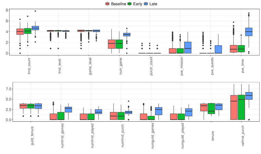
Figure 3: Box plot of the $16$ playing characteristics on day 5. Data are arcsinh transformed and the variable pve_time is reported in hours. Here $m_{1}=143$, $m_{2}=216$ and $n=2,340$. See Table 11 in Supplementary Section D for a description of these characteristics.

Figure 3 provides a box-plot of the 16 playing characteristics on day 5. It reveals that Late players seem to play relatively larger number of games (num_games), spend more time playing with the game environment (pve_quests and pve_time) and are relatively more engaged with their friends and social connections within the game (numfrnd-games,numfrnd-played, numguild-played) than their counterparts in Baseline. The Early players, on the other hand, do not exhibit such stark contrasts in their playing behavior when compared to the Baseline. A t-SNE plot (Van der Maaten and Hinton, 2008) of the $d=16$ dimensional data in figures 5 and 5 provide further insights into the behavior of the Late and Early players. For both days 1 and 4, these figures exhibit the underlying heterogeneity in the Baseline player sample. Moreover, the Late sample occupies a distinct position in the two dimensional space that is away from the bulk of the Baseline sample.

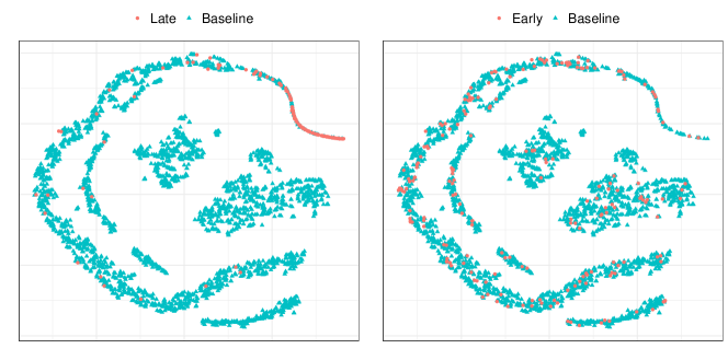
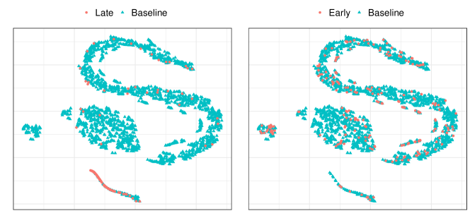
Figure 4: A t-SNE plot of the data for Day 1. The $d=16$ playing attributes are projected to a two dimensional space.

Figure 5: A t-SNE plot of the data for Day 4. The $d=16$ playing attributes are projected to a two dimensional space.

Tables 5 and 6 report the $p-$values for the two testing problems. In Table 5, all competing tests, with the exception of TRUH, reject the null hypothesis $H_{01}:F^{(1)}_{\bm{Y}_{1}}\in\mathcal{F}(F_{\bm{X}})$ across the $7$ days and conclude that the playing behavior of the Late players is significantly different from Baseline. This corroborates the visual evidence found in figures 3, 5 and 5 that indeed the players who login late differ from their counterparts in Baseline as far as these $16$ playing characteristics are concerned.

Table 5: $p-$values for testing $H_{01}:F^{(1)}_{\bm{Y}_{1}}\in\mathcal{F}(F_{\bm{X}})~{}vs~{}H_{11}:F^{(1)}_{\bm{Y}_{1}}\notin\mathcal{F}(F_{\bm{X}})$

Day	$n$	$m_{1}$	EC test	GEC test	WEC test	TRUH	BGEC test	BWEC test
1	$2,558$	$133$	$<10^{-3}$	$<10^{-3}$	$<10^{-3}$	$1.000$	$<10^{-3}$	$<10^{-3}$
2	$2,374$	$103$	$<10^{-3}$	$<10^{-3}$	$<10^{-3}$	$<10^{-3}$	$<10^{-3}$	$<10^{-3}$
3	$2,073$	$163$	$<10^{-3}$	$<10^{-3}$	$<10^{-3}$	$1.000$	$<10^{-3}$	$<10^{-3}$
4	$2,291$	$126$	$<10^{-3}$	$<10^{-3}$	$<10^{-3}$	$<10^{-3}$	$<10^{-3}$	$<10^{-3}$
5	$2,340$	$143$	$<10^{-3}$	$<10^{-3}$	$<10^{-3}$	$1.000$	$<10^{-3}$	$<10^{-3}$
6	$2,560$	$72$	$<10^{-3}$	$<10^{-3}$	$<10^{-3}$	$1.000$	$<10^{-3}$	$<10^{-3}$
7	$2,268$	$140$	$<10^{-3}$	$<10^{-3}$	$<10^{-3}$	$<10^{-3}$	$<10^{-3}$	$<10^{-3}$

Table 6: $p-$values for testing $H_{02}:F^{(2)}_{\bm{Y}_{2}}\in\mathcal{F}(F_{\bm{X}})~{}vs~{}H_{12}:F^{(2)}_{\bm{Y}_{2}}\notin\mathcal{F}(F_{\bm{X}})$

Day	$n$	$m_{2}$	EC test	GEC test	WEC test	TRUH	BGEC test	BWEC test
1	$2,558$	$203$	$0.702$	$<10^{-3}$	$<10^{-3}$	$0.525$	$0.863$	$0.917$
2	$2,374$	$223$	$0.193$	$<10^{-3}$	$<10^{-3}$	$0.995$	$1.000$	$1.000$
3	$2,073$	$171$	$0.864$	$0.001$	$0.002$	$0.715$	$1.000$	$1.000$
4	$2,291$	$232$	$<10^{-3}$	$<10^{-3}$	$<10^{-3}$	$0.795$	$1.000$	$1.000$
5	$2,340$	$216$	$<10^{-3}$	$<10^{-3}$	$<10^{-3}$	$0.105$	$0.995$	$0.998$
6	$2,560$	$177$	$0.487$	$<10^{-3}$	$<10^{-3}$	$0.890$	$1.000$	$1.000$
7	$2,268$	$199$	$0.708$	$<10^{-3}$	$<10^{-3}$	$0.855$	$0.978$	$0.988$

TRUH, on the other hand, does not provide such a consistent picture across the seven days and fails to reject $H_{01}$ in four out of the seven days. The numerical experiments of Section 4 reveal that TRUH is relatively less powerful than BGEC and BWEC tests in detecting departures from $H_{01}$ and the result in Table 5 is potentially another empirical evidence in that direction. The $p-$values reported in Table 6 exhibit an interesting pattern for the testing problem $H_{02}:F^{(2)}_{\bm{Y}_{2}}\in\mathcal{F}(F_{\bm{X}})~{}vs~{}H_{12}:F^{(2)}_{\bm{Y}_{2}}\notin\mathcal{F}(F_{\bm{X}})$. We note that TRUH, BWEC and BGEC tests fail to reject $H_{02}$ across the seven days, while the decisions from GEC and WEC tests are exactly the opposite, potentially demonstrating the non-conservativeness of these tests for testing the composite null hypothesis $H_{02}$. On five out of the seven days, EC test fails to reject $H_{02}$ and gives the impression that it is conservative for testing $H_{02}$. However, and as observed in Section 4, at moderately high dimensions the EC test statistic suffers from variance boosting under sample size imbalance and demonstrates low power.

6 Discussion

The multivariate samples from modern gargantuan datasets often involve heterogeneity and direct application of existing nonparametric two-sample tests, such as the edge count tests, may lead to incorrect scientific decisions if they are not properly calibrated for the underlying latent heterogeneity. In this article, we demonstrate that under a composite null hypothesis, that allows the possibility that two samples may originate from the same mixture distribution but with possibly different mixing weights, the weighted edge count test can be re-calibrated to obtain a test which is asymptotically powerful for general alternatives. For practical implementation of this test, we develop a bootstrap calibrated weighted edge count test and demonstrate its excellent finite sample properties across a wide range of simulation studies. On a real world video game dataset, we use our testing procedure to detect addictive playing behavior and find that in comparison to players who exhibit normal playing behavior, players who login late to the game exhibit aberrant behavior while players who login early do not, thus confirming some of the findings in existing literature related to video game addiction.

Our future research will be directed towards extending the proposed testing framework in two directions. First, it will be interesting to develop an extension of the kernel two-sample tests of Gretton et al. (2007) to the heterogeneous setting and devise an efficient re-calibration procedure for these tests for consistent two-sample testing under the composite null hypothesis of Equation (7). Second, for dealing with samples that involve high dimensional features, such as single cell RNA-seq data where $d\sim 10^{4}$, or data on consumer preferences for high dimensional product attributes, we will be interested in developing an extension of our testing procedure that allows incorporating such data-types into our heterogeneous two-sample testing framework.

SUPPLEMENTARY MATERIAL FOR “Bootstrapped Edge Count Tests for Nonparametric Two-Sample Inference Under Heterogeneity”

This supplement is organized as follows: Section A provides the proof of Proposition 1, Section B includes the simulation scheme for figures 1 and 2, Section C presents an additional simulation setting for the comparing the performance of BWEC, BGEC, and Section D provides the data dictionary for the data used in Section 5.

Appendix A Proof of Proposition 1

Recall from Equation (9) the definition of the Henze-Penrose divergence:

$$\delta_{\rho}(f_{\bm{X}},f_{\bm{Y}})=\int_{S}\frac{\rho f_{\bm{X}}^{2}(x)+f_{\bm{Y}}^{2}(x)}{(\rho f_{\bm{X}}(x)+f_{\bm{Y}}(x))}\mathrm{d}x.$$

We begin with the following lemma:

Lemma 1.

Under the assumptions of Proposition 1, for any $f_{\bm{Y}}\in\mathcal{F}(f_{\bm{X}})$,

$$\delta_{\rho}(f_{\bm{X}},f_{\bm{Y}})<1+\frac{(1+\rho)K^{2}}{L\rho^{2}}.$$

Proof: Define the function $r_{\rho}:\mathbb{R}_{\geq 0}^{2}\rightarrow\mathbb{R}_{\geq 0}$ as:

$$r_{\rho}(s,t)=\frac{\rho s^{2}+t^{2}}{(\rho s+t)}.$$

Note that $\delta_{\rho}(f_{\bm{X}},f_{\bm{Y}})=\int_{S}r_{\rho}(f_{\bm{X}}(x),f_{\bm{Y}}(x))\mathrm{d}x$. By a Taylor series expansion of the function $t\rightarrow r_{\rho}(f_{\bm{X}}(x),t)$ we can write,

$$r_{\rho}(f_{\bm{X}}(x),f_{\bm{Y}}(x))-r_{\rho}(f_{\bm{X}}(x),f_{\bm{X}}(x))$$

$$=\frac{\partial}{\partial t}r_{\rho}(f_{\bm{X}}(x),t)\mid_{t=f_{\bm{X}}(x)}(f_{\bm{Y}}(x)-f_{\bm{X}}(x))+\frac{(f_{\bm{Y}}(x)-f_{\bm{X}}(x))^{2}}{2}\frac{\partial^{2}}{\partial t^{2}}r_{\rho}(f_{\bm{X}}(x),t)\mid_{t=\zeta_{x}},$$ (10)

for some $\zeta_{x}\in[f_{\bm{X}}(x)\wedge f_{\bm{Y}}(x),f_{\bm{X}}(x)\vee f_{\bm{Y}}(x)]$. Note that

$$\frac{\partial}{\partial t}r_{\rho}(f_{\bm{X}}(x),t)=\frac{t^{2}+2\rho f_{\bm{X}}(x)t-\rho f_{\bm{X}}(x)^{2}}{(\rho f_{\bm{X}}(x)+t)^{2}}\quad\text{and}\quad\frac{\partial^{2}}{\partial^{2}t}r_{\rho}(s,t)=\frac{2\rho(1+\rho)f_{\bm{X}}(x)^{2}}{(\rho f_{\bm{X}}(x)+t)^{3}}.$$

This implies, $\frac{\partial}{\partial t}r_{\rho}(f_{\bm{X}}(x),t)\mid_{t=f_{\bm{X}}(x)}=\frac{1}{1+\rho}:=c_{\rho}$. Then, using $r_{\rho}(f_{\bm{X}}(x),f_{\bm{X}}(x))=f_{\bm{X}}(x)$ Equation (A) simplifies to

$$r_{\rho}(f_{\bm{X}}(x),f_{\bm{Y}}(x)) =f_{\bm{X}}(x)+c_{\rho}(f_{\bm{Y}}(x)-f_{\bm{X}}(x))+(f_{\bm{Y}}(x)-f_{\bm{X}}(x))^{2}\frac{\rho(1+\rho)f_{\bm{X}}^{2}(x)}{(\rho f_{\bm{X}}(x)+\zeta_{x})^{3}}.$$

Integrating both sides over $x\in S$ and using $\int_{S}f_{\bm{X}}\mathrm{d}x=\int_{S}f_{\bm{Y}}(x)\mathrm{d}x=1$, gives

$$\delta_{\rho}(f_{\bm{X}},f_{\bm{Y}}) =1+\rho(1+\rho)\int_{S}(f_{\bm{Y}}(x)-f_{\bm{X}}(x))^{2}\frac{f_{\bm{X}}^{2}(x)}{(\rho f_{\bm{X}}(x)+\zeta_{x})^{3}}\mathrm{d}x$$ (11)

$$\leq 1+\frac{1+\rho}{\rho^{2}}\int_{S}\frac{(f_{\bm{Y}}(x)-f_{\bm{X}}(x))^{2}}{f_{\bm{X}}(x)}\mathrm{d}x,$$ (12)

where the last step uses $\rho f_{\bm{X}}(x)+\zeta_{x}\geq\rho f_{\bm{X}}(x)$. Now, suppose $f_{\bm{Y}}\in\mathcal{F}(f_{\bm{X}})$, that is, $f_{\bm{Y}}=\sum_{a=1}^{K}\lambda_{a}f_{a}(x)$, for some $\lambda_{1},\lambda_{2},\ldots,\lambda_{K}\in[0,1]$ such that $\sum_{a=1}^{K}\lambda_{a}=1$. Also, recall from Equation (5) that $f_{\bm{X}}=\sum_{a=1}^{K}w_{a}f_{a}(x)$. Then for $f_{\bm{Y}}\in\mathcal{F}(f_{\bm{X}})$ we have from Equation (12),

$$\delta_{\rho}(f_{\bm{X}},f_{\bm{Y}}) =1+\frac{1+\rho}{\rho^{2}}\int_{S}\frac{(\sum_{a=1}^{K}(\lambda_{a}-w_{a})f_{a}(x))^{2}}{\sum_{a=1}^{K}w_{a}f_{a}(x)}\mathrm{d}x$$

$$\leq 1+\frac{(1+\rho)K}{\rho^{2}}\int_{S}\frac{\sum_{a=1}^{K}(\lambda_{a}-w_{a})^{2}f_{a}^{2}(x)}{\sum_{a=1}^{K}w_{a}f_{a}(x)}\mathrm{d}x,$$ (13)

where the last step follows from the Cauchy-Schwarz inequality. Note that by Assumption 2,

$$\sum_{a=1}^{K}w_{a}f_{a}(x)>L\sum_{a=1}^{K}f_{a}(x).$$

Moreover,

$$\sum_{a=1}^{K}(\lambda_{a}-w_{a})^{2}f_{a}^{2}(x)\leq\sum_{a=1}^{K}f_{a}^{2}(x)\leq\left(\sum_{a=1}^{K}f_{a}(x)\right)^{2}.$$

Using the above two bounds in Equation (A) we have,

$$\delta_{\rho}(f_{\bm{X}},f_{\bm{Y}}) <1+\frac{(1+\rho)K}{L\rho^{2}}\int_{S}\sum_{a=1}^{K}f_{a}(x)\mathrm{d}x=1+\frac{(1+\rho)K^{2}}{L\rho^{2}}.$$

This completes the proof of Lemma 1.

To complete the proof of the first statement in Proposition 1 recall from Equation (8) that for $f_{\bm{Y}}\in\mathcal{F}(f_{\bm{X}})$,

$$\mathcal{R}_{w}(\mathcal{X}_{n},\mathcal{Y}_{m})\stackrel{{\scriptstyle P}}{{\to}}\frac{\ell\rho}{(1+\rho)^{2}}\cdot\delta_{\rho}(f_{\bm{X}},f_{\bm{Y}})<\frac{\ell\rho}{(1+\rho)^{2}}\left(1+\frac{(1+\rho)K^{2}}{L\rho^{2}}\right):=\gamma.$$ (14)

This implies,

$$\lim_{m,n\rightarrow\infty}\mathbb{P}_{f_{\bm{X}},f_{\bm{Y}}}(\mathcal{R}_{w}(\mathcal{X}_{n},\mathcal{Y}_{m})>\gamma)=0,$$

for $f_{\bm{Y}}\in\mathcal{F}(f_{\bm{X}})$.

For proving the second statement in Proposition 1, using $\zeta_{x}\in[f_{\bm{X}}(x)\wedge f_{\bm{Y}}(x),f_{\bm{X}}(x)\vee f_{\bm{Y}}(x)]$ and Assumption 1 in Equation (11) we have,

$$\delta_{\rho}(f_{\bm{X}},f_{\bm{Y}}) =1+\rho(1+\rho)\int_{S}(f_{\bm{Y}}(x)-f_{\bm{X}}(x))^{2}\frac{f_{\bm{X}}^{2}(x)}{(\rho f_{\bm{X}}(x)+\zeta_{x})^{3}}\mathrm{d}x$$

$$\geq 1+\rho(1+\rho)\int_{S}(f_{\bm{Y}}(x)-f_{\bm{X}}(x))^{2}\frac{f_{\bm{X}}^{2}(x)}{(\rho f_{\bm{X}}(x)+f_{\bm{X}}(x)\vee f_{\bm{Y}}(x))^{3}}\mathrm{d}x$$

$$\geq 1+\frac{\rho}{M_{2}^{3}(1+\rho)^{2}}\int_{S}(f_{\bm{Y}}(x)-f_{\bm{X}}(x))^{2}f_{\bm{X}}^{2}(x)\mathrm{d}x$$ (15)

$$\geq 1+\frac{\rho M_{1}^{2}}{M_{2}^{3}(1+\rho)^{2}}\int_{S}(f_{\bm{Y}}(x)-f_{\bm{X}}(x))^{2}\mathrm{d}x.$$ (16)

Note that the bound in Equation (15) uses $\sup_{x\in S}\left\{\rho f_{\bm{X}}(x)+f_{\bm{X}}(x)\vee f_{\bm{Y}}(x))\right\}\leq M_{2}(1+\rho)$ and the bound in Equation (16) uses $f_{\bm{X}}(x)\geq M_{1}$, for all $x\in S$, by Assumption 1.

Now, if $f_{\bm{Y}}\notin\mathcal{F}(f_{\bm{X}})$ is such that $\int_{S}(f_{\bm{Y}}(x)-f_{\bm{X}}(x))^{2}\mathrm{d}x\geq\varepsilon^{2}:=\frac{2M_{2}^{3}(1+\rho)^{3}K^{2}}{M_{1}^{2}\rho^{3}L}$, then

$$\mathcal{R}_{w}(\mathcal{X}_{n},\mathcal{Y}_{m})\stackrel{{\scriptstyle P}}{{\to}}\frac{\ell\rho}{(1+\rho)^{2}}\cdot\delta_{\rho}(f_{\bm{X}},f_{\bm{Y}})\geq\gamma+\frac{\ell K^{2}}{L\rho(1+\rho)},$$

for $\gamma$ as defined in Equation (14). Therefore,

$$\lim_{m,n\rightarrow\infty}\mathbb{P}_{f_{\bm{X}},f_{\bm{Y}}}(\mathcal{R}_{w}(\mathcal{X}_{n},\mathcal{Y}_{m})>\gamma)=1,$$ (17)

for $f_{\bm{Y}}\notin\mathcal{F}(f_{\bm{X}})$ such that $\int_{S}(f_{\bm{Y}}(x)-f_{\bm{X}}(x))^{2}\mathrm{d}x\geq\varepsilon^{2}$. $\Box$

Remark 2.

In the proof of Proposition 1 the assumption that $f_{\bm{X}}$ is bounded away from zero is used in Equation (16). This assumption can be removed if instead we assume that there exists $\kappa>0$ such that the truncated $L_{2}$-distance:

$$\int_{\{f_{\bm{X}}(x)>\kappa\}}(f_{\bm{Y}}(x)-f_{\bm{X}}(x))^{2}\geq\tilde{\varepsilon}^{2}/\kappa^{2},$$ (18)

where $\tilde{\varepsilon}^{2}:=\frac{2M_{2}^{3}(1+\rho)^{3}K^{2}}{\rho^{3}L}$. To see this, note from Equation (15) that for any $\kappa>0$,

$$\delta_{\rho}(f_{\bm{X}},f_{\bm{Y}}) \geq 1+\frac{\rho}{M_{2}^{3}(1+\rho)^{2}}\int_{S}(f_{\bm{Y}}(x)-f_{\bm{X}}(x))^{2}f_{\bm{X}}^{2}(x)\mathrm{d}x$$

$$\geq 1+\frac{\rho\kappa^{2}}{M_{2}^{3}(1+\rho)^{2}}\int_{\{f_{\bm{X}}(x)>\kappa\}}(f_{\bm{Y}}(x)-f_{\bm{X}}(x))^{2}\mathrm{d}x\geq 1+\frac{2(1+\rho)K^{2}}{L\rho^{2}},$$

where the last inequality uses Equation (18) and the definition of $\varepsilon$. This implies,

$$\mathcal{R}_{w}(\mathcal{X}_{n},\mathcal{Y}_{m})\stackrel{{\scriptstyle P}}{{\to}}\frac{\ell\rho}{(1+\rho)^{2}}\cdot\delta_{\rho}(f_{\bm{X}},f_{\bm{Y}})\geq\gamma+\frac{\ell K^{2}}{L\rho(1+\rho)}.$$

Therefore, Equation (17) holds whenever the truncated $L_{2}$-condition in Equation (18) is satisfied.

Appendix B Details for figures 1 and 2

We next describe the two simulation settings that were discussed in Section 1.1 under examples 1, 2 and figures 1, 2. For Example 1 and Figure 1, we fix $n=2000,~{}m=200,~{}d=2$ and let $F_{\bm{X}}=\sum_{k=1}^{4}w_{k}\mathcal{N}_{d}(\bm{\mu}_{k},\bm{I}_{d})$ where $w_{k}=0.25$ for $k=1,\ldots,4$, $\bm{\mu}_{1}=(10,10)$, $\bm{\mu}_{2}=(20,10)$, $\bm{\mu}_{3}=(20,20)$ and $\bm{\mu}_{4}=(10,20)$. We consider three scenarios for simulating $\mathcal{Y}_{m}$ from $F_{\bm{Y}}$. For Case I, we let $F_{\bm{Y}}=F_{\bm{X}}$ and ,thus, $F_{\bm{Y}}\in\mathcal{F}(F_{\bm{X}})$ since $F_{\bm{Y}}$ has all the subpopulations present in $F_{\bm{X}}$. In Case II, we consider $F_{\bm{Y}}=0.1\,\mathcal{N}_{d}(\bm{\mu}_{1},\bm{I}_{d})+0.8\,\mathcal{N}_{d}(\bm{\mu}_{2},\bm{I}_{d})+0.1\,\mathcal{N}_{d}(\bm{\mu}_{3},\bm{I}_{d})$. So, $F_{\bm{Y}}\in\mathcal{F}(F_{\bm{X}})$ since $F_{\bm{Y}}$ has all the subpopulations present in $F_{\bm{X}}$ but at different proportions. Finally, for Case III we let $F_{\bm{Y}}=\mathcal{N}_{d}(\bm{\mu}_{5},\bm{I}_{d})$ where $\bm{\mu}_{5}=(25,5)$. This setting presents a scenario where $F_{\bm{Y}}\notin\mathcal{F}(F_{\bm{X}})$ and the composite null $H_{0}$ is not true. Table 7 reports the rejection rates for testing $H_{0}:F_{\bm{Y}}\in\mathcal{F}(F_{\bm{X}})~{}vs~{}H_{1}:F_{\bm{Y}}\notin\mathcal{F}(F_{\bm{X}})$ under the three scenarios described in Example 1 and Figure 1. We note that the three edge count tests cannot distinguish Case II from Case III and infer $F_{\bm{Y}}\notin\mathcal{F}(F_{\bm{X}})$ for both these cases.

Table 7: Rejection rates at $5\%$ level of significance: Example 1 and Figure 1 in Section 1.1.

	$n=2000,~{}m=200,~{}d=2$
Method	Left panel	Center panel	Right panel
	Case I - $F_{\bm{Y}}\in\mathcal{F}(F_{\bm{X}})$	Case II - $F_{\bm{Y}}\in\mathcal{F}(F_{\bm{X}})$	Case III - $F_{\bm{Y}}\notin\mathcal{F}(F_{\bm{X}})$
EC test	0.048	1.000	1.000
GEC test	0.032	1.000	1.000
WEC test	0.056	1.000	1.000
TRUH test	0.048	0.058	1.000
BGEC test	0.000	0.000	1.000
BWEC test	0.000	0.000	1.000

For Example 2 and Figure 2, we take $d=3$ and let $F_{\bm{X}}=\sum_{k=1}^{3}w_{k}\mathcal{N}_{d}(\bm{\mu}_{k},\bm{I}_{d})$ where $w_{1}=w_{2}=0.3,~{}w_{3}=0.4$, $\bm{\mu}_{1}=(0,0,0)$, $\bm{\mu}_{2}=(0,-4,-4)$, and $\bm{\mu}_{3}=(4,-2,-3)$. We consider three scenarios for simulating $\mathcal{Y}_{m}$ from $F_{\bm{Y}}$. In Case I, we let $F_{\bm{Y}}=F_{\bm{X}}$ and, thus, $F_{\bm{Y}}\in\mathcal{F}(F_{\bm{X}})$. For Case II, we consider $F_{\bm{Y}}=0.8\,\mathcal{N}_{d}(\bm{\mu}_{1},\bm{I}_{d})+0.1\,\mathcal{N}_{d}(\bm{\mu}_{2},\bm{I}_{d})+0.1\,\mathcal{N}_{d}(\bm{\mu}_{3},\bm{I}_{d})$. So, $F_{\bm{Y}}\in\mathcal{F}(F_{\bm{X}})$ since $F_{\bm{Y}}$ has all the subpopulations present in $F_{\bm{X}}$ but at different proportions. In Case III, we let $F_{\bm{Y}}=0.8\,\mathcal{N}_{d}(\bm{\mu}_{1},\bm{\Sigma}_{d})+0.1\,\mathcal{N}_{d}(\bm{\mu}_{2},\bm{\Sigma}_{d})+0.1\,\mathcal{N}_{d}(\bm{\mu}_{3},\bm{\Sigma}_{d})$ where $\bm{\Sigma}_{d}=0.1\bm{I}_{d}$. This setting presents a scenario where $F_{\bm{Y}}\notin\mathcal{F}(F_{\bm{X}})$ since the components of $F_{\bm{Y}}$ differ from the components of $F_{\bm{X}}$ with respect to their scale parameters. Table 8 reports the rejection rates for testing $H_{0}:F_{\bm{Y}}\in\mathcal{F}(F_{\bm{X}})~{}vs~{}H_{1}:F_{\bm{Y}}\notin\mathcal{F}(F_{\bm{X}})$ under the three scenarios described in Example 2 and Figure 2. We continue to note that the three edge count tests cannot distinguish Case II from Case III and infer $F_{\bm{Y}}\notin\mathcal{F}(F_{\bm{X}})$ for both these cases. This suggests that the edge count tests are unable to tackle subpopulation level heterogeneity. Additionally, the TRUH test incorrectly infers $F_{\bm{Y}}\in\mathcal{F}(F_{\bm{X}})$ for Case III, thus demonstrating low power for detecting departures from $H_{0}$ when the components of $F_{\bm{Y}}$ and $F_{\bm{X}}$ differ only with respect to their scales.

Table 8: Rejection rates at $5\%$ level of significance: Example 2 and Figure 2 in Section 1.1.

	$n=2000,~{}m=200,~{}d=3$
Method	Left panel	Center panel	Right panel
	Case I - $F_{\bm{Y}}\in\mathcal{F}(F_{\bm{X}})$	Case II - $F_{\bm{Y}}\in\mathcal{F}(F_{\bm{X}})$	Case III - $F_{\bm{Y}}\notin\mathcal{F}(F_{\bm{X}})$
EC test	0.068	1.000	1.000
GEC test	0.068	1.000	1.000
WEC test	0.064	1.000	1.000
TRUH test	0.012	0.018	0.004
BGEC test	0.000	0.000	1.000
BWEC test	0.000	0.000	1.000

Appendix C Numerical experiment 3

We consider a setting where the samples $\mathcal{X}_{n}$ and $\mathcal{Y}_{m}$ exhibit zero inflation across the $d$ dimensions. Denote $\bm{\delta}_{\{\bm{0}\}}=(\delta_{1\{0\}},\ldots,\delta_{d\{0\}})$ denote the $d-$dimensional vector of point masses at $0$. We let $F_{\bm{X}}=\bm{p}\delta_{\{\bm{0}\}}+(\bm{1}_{d}-\bm{p})~{}\Bigl{\{}0.5~{}F_{1}+0.5~{}F_{2}\Bigr{\}},$ where $F_{1}={\mathrm{Gam}}_{d}(\text{shape}=5\bm{1}_{d},\text{rate}=\bm{1}_{d},\bm{\Sigma}_{1})$, $F_{2}={\mathrm{Exp}}_{d}(\text{rate}=\bm{1}_{d},\bm{\Sigma}_{2})$ and $\bm{p}=(p_{1},\ldots,p_{d})$ is the vector of probabilities that regulate the differential zero inflation across the $d$ dimensions. We sample the first $0.8d$ coordinates of $\bm{p}$ independently from $\text{Unif}(0.5,0.6)$, and the remaining $0.2d$ coordinates are set to $0$. So the first $0.8d$ coordinates of $F_{\bm{X}}$ encounter zero inflation. Finally, $\bm{\Sigma}_{1},\bm{\Sigma}_{2}$ are as described in Experiment 2 (Section 4.2) and $\mathcal{X}_{n}$ are sampled from $F_{\bm{X}}$ using the R-package lcmix. For simulating $\mathcal{Y}_{m}$ from $F_{\bm{Y}}$, we consider the following two scenarios:

• Scenario I: $F_{\bm{Y}}=\bm{p}\bm{\delta}_{\{\bm{0}\}}+(\bm{1}_{d}-\bm{p})~{}\{0.2~{}F_{1}+0.8~{}F_{2}\}$ and so $H_{0}:F_{\bm{Y}}\in\mathcal{F}(F_{\bm{X}})$ is true.

• Scenario II: $F_{\bm{Y}}=\bm{q}\delta_{\{\bm{0}\}}+(\bm{1}_{d}-\bm{q})~{}\{0.5~{}{\mathrm{Gam}}_{d}(\text{shape}=5\bm{1}_{d},\text{rate}=1.5\bm{1}_{d},\bm{\Sigma}_{1})+0.5~{}F_{2}\}$, where the first $0.8d$ coordinates of $\bm{q}$ are set to $0.3$ and the remaining $0.2d$ coordinates to $0$. Apart from the differential zero inflation between $F_{\bm{Y}}$ and $F_{\bm{X}}$, the rate parameter of the first component of $F_{\bm{Y}}$ is different from that of $F_{1}$. So in this scenario, $G\notin\mathcal{F}(F_{0})$ and $H_{0}$ is false.

Table 9: Rejection rates at $5\%$ level of significance: Experiment 3 and Scenario 1 wherein $H_{0}:F_{\bm{Y}}\in\mathcal{F}(F_{\bm{X}})$ is true.

	$n=500,~{}m=50$			$n=2000,~{}m=200$
Method	$d=5$	$d=15$	$d=30$	$d=5$	$d=15$	$d=30$
EC test	0.070	0.074	0.024	0.302	0.140	0.102
GEC test	0.264	0.284	0.256	0.624	0.680	0.752
WEC test	0.352	0.408	0.392	0.790	0.830	0.880
TRUH test	0.002	0.000	0.000	0.000	0.000	0.000
BGEC test	0.046	0.000	0.000	0.000	0.000	0.000
BWEC test	0.058	0.000	0.000	0.000	0.000	0.000

Table 9 reports the rejection rates for the competing tests under Scenario I and reveals that under the setting of zero inflation, the WEC and GEC tests are not conservative. TRUH, BWEC and BGEC tests, on the other hand, report rejection rates that are either at or below the prespecified $0.05$ level, thus demonstrating their conservatism in testing $H_{0}:F_{\bm{Y}}\in\mathcal{F}(F_{\bm{X}})~{}vs~{}H_{1}:F_{\bm{Y}}\notin\mathcal{F}(F_{\bm{X}})$.

Table 10: Rejection rates at $5\%$ level of significance: Experiment 3 and Scenario 2 wherein $H_{0}:F_{\bm{Y}}\in\mathcal{F}(F_{\bm{X}})$ is false.

	$n=500,~{}m=10$			$n=2000,~{}m=40$
Method	$d=5$	$d=15$	$d=30$	$d=5$	$d=15$	$d=30$
EC test	0.106	0.000	0.000	0.420	0.000	0.000
GEC test	0.250	0.604	0.878	0.732	0.986	1.000
WEC test	0.344	0.526	0.704	0.828	0.978	1.000
TRUH test	0.012	0.004	0.012	0.008	0.000	0.000
BGEC test	0.124	0.390	0.772	0.198	0.874	0.998
BWEC test	0.138	0.288	0.512	0.196	0.822	0.986

In Table 10 we report the rejection rates for Scenario II when the sample size imbalance is $0.02$ as opposed to $0.1$ in Scenario I. Under this challenging setting, we find that BWEC and BGEC tests are more powerful than TRUH and demonstrate competitive power to WEC and GEC tests when the sample sizes are relatively large. Table 9 gives the impression that at $d=30$, the EC test is conservative for testing $H_{0}$ under Scenario I. However, at such moderately high dimensions and under unequal sample sizes, the edgecount test statistic suffers from variance boosting and demonstrates low power, which explains its relatively low rejection rates in both tables 9 and 10.

Appendix D Data dictionary

Table 11 provides a description of the $d=16$ player characteristics available in the video game data used in Section 5.

Table 11: Data dictionary

Sl no.	Variable name	Description
1	game_level	player’s level in the game
2	pve_quests	no. of quests a player accomplished in Player Versus Environment (PVE) mode
3	pve_mission	no. of missions a player accomplished in PVE mode
4	pve_time	player’s daily time spent in playing PVE mode in hours
5	num_game	no. of PVE game rounds a player played in a day
6	purch_count	no. of purchases a player made in a day
7	frnd_count	no. of friends a player has
8	frnd_level	mean level of a player’s friends
9	numfrnd_purch	no. of times of a player’s friends made purchases
10	valfrnd_purch	monetary value of all purchases made by a player’s friends
11	numfrnd_played	no. of friends a player played with during game sessions
12	numfrnd_games	no. of game sessions a player played with her friends
13	tenure	no. of days a player has been associated with the game
14	guild_tenure	no. of days a player has been associated with a guild
15	numguild_played	no. of guild members a player played with
16	numguild_games	no. of game sessions a player played with guild members

References

- Agarwal et al. (2019) Sumit Agarwal, Pulak Ghosh, Jing Li, and Tianyue Ruan. Digital payments induce over-spending: Evidence from the 2016 demonetization in india. 2019. URL https://abfer.org/media/abfer-events-2019/annual-conference/economic-transformation-of-asia/AC19P4028_Digital_Payments_Induce_Excessive_Spending_Evidence_from_Demonetization_in_India.pdf.
- Akpan et al. (2022) Ikpe Justice Akpan, Elijah Abasifreke Paul Udoh, and Bamidele Adebisi. Small business awareness and adoption of state-of-the-art technologies in emerging and developing markets, and lessons from the covid-19 pandemic. Journal of Small Business & Entrepreneurship, 34(2):123–140, 2022.
- Aslan and Zech (2005) B Aslan and G Zech. New test for the multivariate two-sample problem based on the concept of minimum energy. Journal of Statistical Computation and Simulation, 75(2):109–119, 2005.
- Balis (2021) Janet Balis. 10 truths about marketing after the pandemic. 2021. URL https://hbr.org/2021/03/10-truths-about-marketing-after-the-pandemic.
- Banerjee et al. (2020) Trambak Banerjee, Bhaswar B Bhattacharya, and Gourab Mukherjee. A nearest-neighbor based nonparametric test for viral remodeling in heterogeneous single-cell proteomic data. Annals of Applied Statistics, 14(4):1777–1805, 2020.
- Banerjee et al. (2022) Trambak Banerjee, Peng Liu, Gourab Mukherjee, Shantanu Dutta, and Hai Che. Joint modeling of playing time and purchase propensity in massively multiplayer online role playing games using crossed random effects. 2022. URL https://gmukherjee.github.io/pdfs/crejm.pdf.
- Baringhaus and Franz (2004) Ludwig Baringhaus and Carsten Franz. On a new multivariate two-sample test. Journal of multivariate analysis, 88(1):190–206, 2004.
- Bartik et al. (2020) Alexander W Bartik, Marianne Bertrand, Zoe Cullen, Edward L Glaeser, Michael Luca, and Christopher Stanton. The impact of covid-19 on small business outcomes and expectations. Proceedings of the national academy of sciences, 117(30):17656–17666, 2020.
- Bhattacharya (2019) Bhaswar B Bhattacharya. A general asymptotic framework for distribution-free graph-based two-sample tests. Journal of the Royal Statistical Society: Series B (Statistical Methodology), 81(3):575–602, 2019.
- Biau and Devroye (2015) Gérard Biau and Luc Devroye. Lectures on the nearest neighbor method, volume 246. Springer, 2015.
- Bickel (1969) Peter J Bickel. A distribution free version of the smirnov two sample test in the p-variate case. The Annals of Mathematical Statistics, 40(1):1–23, 1969.
- Bruun (2021) Kayla Bruun. Supply chain disruptions limit consumer spending. 2021. URL https://morningconsult.com/2021/09/27/supply-chain-disruptions-limit-consumer-spending/.
- Callahan et al. (2016) Ben J Callahan, Kris Sankaran, Julia A Fukuyama, Paul J McMurdie, and Susan P Holmes. Bioconductor workflow for microbiome data analysis: from raw reads to community analyses. F1000Research, 5, 2016.
- Chen and Friedman (2017) Hao Chen and Jerome H Friedman. A new graph-based two-sample test for multivariate and object data. Journal of the American statistical association, 112(517):397–409, 2017.
- Chen and Zhang (2015) Hao Chen and Nancy Zhang. Graph-based change-point detection. The Annals of Statistics, 43(1):139–176, 2015.
- Chen et al. (2018) Hao Chen, Xu Chen, and Yi Su. A weighted edge-count two-sample test for multivariate and object data. Journal of the American Statistical Association, 113(523):1146–1155, 2018.
- Chen et al. (2013) Lisha Chen, Winston Wei Dou, and Zhihua Qiao. Ensemble subsampling for imbalanced multivariate two-sample tests. Journal of the American Statistical Association, 108(504):1308–1323, 2013.
- Chung and Fraser (1958) James H Chung and Donald AS Fraser. Randomization tests for a multivariate two-sample problem. Journal of the American Statistical Association, 53(283):729–735, 1958.
- Chwialkowski et al. (2015) Kacper P Chwialkowski, Aaditya Ramdas, Dino Sejdinovic, and Arthur Gretton. Fast two-sample testing with analytic representations of probability measures. Advances in Neural Information Processing Systems, 28, 2015.
- Conradsen et al. (2003) Knut Conradsen, Allan Aasbjerg Nielsen, Jesper Schou, and Henning Skriver. A test statistic in the complex wishart distribution and its application to change detection in polarimetric sar data. IEEE Transactions on Geoscience and Remote Sensing, 41(1):4–19, 2003.
- Crouzet et al. (2019) Nicolas Crouzet, Apoorv Gupta, and Filippo Mezzanotti. Shocks and technology adoption: Evidence from electronic payment systems. Techn. rep., Northwestern University Working Paper, 2019.
- Deb and Sen (2021) Nabarun Deb and Bodhisattva Sen. Multivariate rank-based distribution-free nonparametric testing using measure transportation. Journal of the American Statistical Association, pages 1–16, 2021.
- Dvorkin (2012) Daniel Dvorkin. lcmix: Layered and chained mixture models, 2012. URL https://R-Forge.R-project.org/projects/lcmix/. R package version 0.3/r5.
- Fahey et al. (2007) Michael T Fahey, Christopher W Thane, Gemma D Bramwell, and W Andy Coward. Conditional gaussian mixture modelling for dietary pattern analysis. Journal of the Royal Statistical Society: Series A (Statistics in Society), 170(1):149–166, 2007.
- Farris and Schopflocher (1999) Karen B Farris and Donald P Schopflocher. Between intention and behavior: an application of community pharmacists’ assessment of pharmaceutical care. Social science & medicine, 49(1):55–66, 1999.
- Folkes et al. (1987) Valerie S Folkes, Susan Koletsky, and John L Graham. A field study of causal inferences and consumer reaction: the view from the airport. Journal of consumer research, 13(4):534–539, 1987.