Some Asymptotic Properties of the Erlang-C Formula
in Many-Server Limiting Regimes

Abstract

This paper presents asymptotic properties of the Erlang-C formula in a spectrum of many-server limiting regimes. Specifically, we address an important gap in the literature regarding its limiting value in critically loaded regimes by studying extensions of the well-known square-root safety staffing rule used in the Quality-and-Efficiency-Driven (QED) regime.

[label1]organization=Smith School of Business at Queen’s University, addressline=143 Union Street West, city=Kingston, postcode=ON K7L 3N6, country=Canada [label2]organization=The University of Chicago Booth School of Business, addressline=5807 S Woodlawn Ave, city=Chicago, postcode=IL 60637, country=United States

1 Introduction

Multiserver systems are widely used to model situations in which customers may be served by one among multiple servers. Classical examples of such systems include call centers [8, 25, 9, 6, 1], healthcare delivery [12, 26, 3], and communication systems [2, 16]. The most basic multiserver queueing model is the $M$/$M$/$N$ queue (also known as the Erlang delay model), where customers arrive according to a Poisson process with rate $\lambda$ and are served by one of $N$ parallel servers for an exponentially distributed amount of time with mean $1/\mu$. A newly arriving customer that finds all servers busy joins a first-come-first-served queue and waits for their turn. Let $\rho=\lambda/\mu$ be the offered load.

A fundamental performance measure of any queueing model is the steady-state probability of delay, i.e., the steady-state probability that an incoming customer does not find an available server immediately upon entry and must therefore wait for service. For the $M$/$M$/$N$ queue, this quantity is given by the well-known Erlang-C formula [7, p.91]:

$$C\left(N,\rho\right)=\frac{\rho^{N}}{N!}\left(\left(1-\frac{\rho}{N}\right)\sum_{i=0}^{N-1}\frac{\rho^{i}}{i!}+\frac{\rho^{N}}{N!}\right)^{-1}.$$ (1)

The Erlang-C formula is heavily relied upon in a wide range of optimization problems in many-server queueing systems, such as optimal staffing problems; see, e.g., [9, 5] and references within. However, finding closed-form solutions for such problems is intractable due to the complexity of the Erlang-C formula. One approach to tackle this challenge is by developing approximations for finite systems [14, 18, 22]. However, more accurate approximations tend to be more analytically complicated, which can be a disadvantage of this method [22]. Alternatively, motivated by large-scale service systems, many-server limits (as $N$ and $\rho$ grow large while $\mu$ remains fixed) have been used to develop analytically simpler approximations [23].

For the $M$/$M$/$N$ queue, the seminal paper [13] shows that, when $N$ and $\rho$ grow unboundedly according to the relationship $N=\rho+\beta\sqrt{\rho}$ for some fixed $\beta>0$, the steady-state probability of delay, namely, the Erlang-C formula (1), converges to a value that is strictly between $0$ and $1$. This relationship is known as the square-root safety staffing rule. It achieves high system utilization, since $\rho/N$ grows closer to its critical value $1$ (and therefore this staffing rule belongs to the class of critically loaded staffing rules), yet short customer waiting time on the order of $1/\sqrt{N}$ [13]. In other words, the square-root safety staffing rule achieves a balance between the dual goals of system efficiency and quality of service. Thus, large-scale systems under the square-root staffing rule are said to operate in the Quality-and-Efficiency-Driven (QED) many-server heavy-traffic limiting regime. Henceforth, we use the terms “square-root safety staffing rule” and “QED regime” interchangeably.

The QED regime is, in fact, the only limiting regime in which the steady-state probability of delay in the $M$/$M$/$N$ queue admits a non-degenerate limit (i.e., a limit that is neither $0$ nor $1$) [13]. Furthermore, it is asymptotically optimal to operate the $M$/$M$/$N$ queue in the QED regime for large and heavily loaded systems, when choosing the optimal staffing level that minimizes a linear combination of staffing and waiting costs or when choosing the smallest staffing level subject to an upper bound on the waiting cost [5].

However, there exist several other well-motivated objectives in the $M$/$M$/$N$ queue and related variants for which the square-root safety staffing is not always asymptotically optimal [19, 11, 28, 30], even among critically loaded staffing policies [20, 17].

In this paper, we address an important gap in the literature regarding the limiting value of the Erlang-C formula under critically loaded staffing rules, by studying extensions of the well-known square-root safety staffing rule, $N=\rho+\beta\sqrt{\rho}$. Specifically, we make the following two inclusions concerning the second-order term in this staffing rule:

1. It can be any sublinear term.

2. It can be negative, i.e., the system can be understaffed (resulting in insufficient capacity to meet the offered load). This is motivated by systems in which customers are lost because they are turned away upon arrival due to fully occupied waiting rooms and/or because they become impatient while in the system and leave before their service is completed (see [9] and the references therein).

In doing so, we identify more staffing rules (in addition to the square-root safety staffing rule) under which the Erlang-C formula admits a non-degenerate limit, making studying the limiting properties of key performance measures of these staffing rules more tractable; see Section 3. This could potentially improve optimal system design by aiding the exploration of an expanded set of candidate staffing rules using many-server heavy-traffic approximations.

Our result unifies all the many-server limiting regimes, including the aforementioned QED regime, the Efficiency-Driven (ED) regime (where $\rho/N$ becomes larger than $1$ in the limit, indicating an overloaded system), and the Quality-Driven (QD) regime (where $\rho/N$ becomes smaller than $1$ in the limit, indicating an underloaded system).

Notation. We conclude this section by introducing some notations that will be used throughout the paper. We use the $o$, $\omega$, and $\Theta$ notations to denote the limiting behavior of functions. Formally, for any two real-valued functions $f(x)$ and $g(x)$ that take nonzero values for all sufficiently large $x$, we say that $f(x)\in o\left(g(x)\right)$ (equivalently, $g(x)\in\omega\left(f(x)\right)$) if $\lim_{x\to\infty}\frac{f(x)}{g(x)}=0$, and $f(x)\in\Theta\left(g(x)\right)$ if $\lim_{x\to\infty}\left|\frac{f(x)}{g(x)}\right|\in(0,\infty)$. Moreover, the relation $f(x)\sim g(x)$ means $\lim_{x\to\infty}\frac{f(x)}{g(x)}=1$. Let $\phi(x)=\frac{1}{\sqrt{2\pi}}e^{-\frac{1}{2}x^{2}}$ and $\Phi^{c}(x)=\int_{x}^{\infty}\phi(t)dt$ denote the probability density function and the complementary cumulative distribution function of the standard normal distribution, respectively. Finally, define $\xi(x):=x\frac{\Phi^{c}(x)}{\phi(x)}$ for $x\in\mathbb{R}$.

2 Main Result

Consider a sequence of systems indexed by the arrival rate $\lambda$, and let $\lambda$ become large. Our convention, when we refer to any process or quantity associated with the system having arrival rate $\lambda$, is to superscript the appropriate symbol by $\lambda$. For example, we denote by $N^{\lambda}$ the number of servers in the system with arrival rate $\lambda$, and $\rho^{\lambda}=\lambda/\mu$ the corresponding offered load. We are interested in many-server limiting regimes obtained by letting the arrival rate $\lambda$ and the number of servers $N^{\lambda}$ grow unboundedly while the service rate $\mu$ remains fixed; nevertheless, our result continues to hold when $N^{\lambda}$ remains bounded as it grows with $\lambda$.

Theorem 1

$$\lim_{\lambda\to\infty}C\big{(}N^{\lambda},\rho^{\lambda}\big{)}=\begin{cases}\infty,&0<\rho^{\lambda}-N^{\lambda}\in\omega(\!\sqrt{\lambda}),\\ \big{(}1-{\color[rgb]{0,0,0}\xi(z)}\big{)}^{-1}\in(1,\infty),&0<\rho^{\lambda}-N^{\lambda}\in\Theta(\!\sqrt{\lambda}),\\ 1,&|N^{\lambda}-\rho^{\lambda}|\in o(\!\sqrt{\lambda}),\\ \big{(}1-{\color[rgb]{0,0,0}\xi(z)}\big{)}^{-1}\in(0,1),&0<N^{\lambda}-\rho^{\lambda}\in\Theta(\!\sqrt{\lambda}),\\ 0,&0<N^{\lambda}-\rho^{\lambda}\in\omega(\!\sqrt{\lambda}),\end{cases}$$

where $z=\lim_{\lambda\to\infty}\frac{\rho^{\lambda}-N^{\lambda}}{\sqrt{N^{\lambda}}}{\color[rgb]{0,0,0}\in\mathbb{R}}$ when $\left|N^{\lambda}-\rho^{\lambda}\right|\in\Theta(\!\sqrt{\lambda})\cup o(\!\sqrt{\lambda})$.

Section 4 is devoted to the proof of Theorem 1.

3 Implications of Theorem 1

In understaffed systems (i.e., when $N^{\lambda}-\rho^{\lambda}$ is negative), the Erlang-C formula (1) loses its interpretation as the steady-state probability of delay in the $M$/$M$/$N$ queue but remains a well-defined mathematical expression that appears in the calculation of key performance measures (KPMs) in extensions of the $M$/$M$/$N$ queue (such as the $M$/$M$/$N$/$k$ and $M$/$M$/$N$+$M$ queues). A central implication of Theorem 1 for such systems is that it can be used to derive limiting approximations of these KPMs that help understand their dependence on the staffing rule. Commonly used KPMs include the steady-state probability of delay [5, 19], probability of abandonment [10], server utilization [29], and expected wait time [27], among others. In this section, we demonstrate how Theorem 1 can be leveraged to obtain the limiting value of the steady-state probability of delay in an $M$/$M$/$N$+$M$ queue (a setting in which square-root safety staffing is not always asymptotically optimal [19]) and briefly discuss the consequent insights regarding the appropriate choice of the staffing rule.

The $M$/$M$/$N$+$M$ queue (also known as the Erlang-A model, first introduced in [21]) extends the $M$/$M$/$N$ queue by allowing customers waiting in queues to renege if they run out of patience before their service begins. The patience time of each customer is independent and identically distributed according to an exponential distribution with mean $1/\theta$. The steady-state probability of delay depends on the Erlang-C formula, as shown next in Lemma 1.

Lemma 1

The steady-state probability of delay in the $M$/$M$/$N$+$M$ queue is given by

$$P(N,\rho;\mu,\theta)=\left(1+\frac{C(N,\rho)^{-1}-1}{\mu(N-\rho)J(N,\rho;\mu,\theta)}\right)^{-1},$$ (2)

where

$$J(N,\rho;\mu,\theta):=\int_{0}^{\infty}e^{\frac{\mu\rho}{\theta}\left(1-e^{-\theta x}\right)-N\mu x}dx.$$ (3)

Furthermore, the quantity $\mu(N-\rho)J(N,\rho;\mu,\theta)$ also admits the following integral representation:

$$\mu(N-\rho)J(N,\rho;\mu,\theta)=1+\frac{\mu\rho}{\theta}\int_{0}^{1}e^{\frac{\mu\rho}{\theta}v}(1-v)^{\frac{N\mu}{\theta}-1}vdv.$$ (4)

Remark 1

Exact expressions for various performance measures in the $M$/$M$/$N$+$M$ and $M$/$M$/$N$+$G$ queues have also been derived in [10, 27].

The proof of Lemma 1 can be found in B.

Theorem 1 can be leveraged to evaluate the limiting value of the steady-state probability of delay (2) under different staffing rules, as we show next in Proposition 1.

Proposition 1 ($\bm{M/M/N}$+$\bm{M}$ Steady-State Delay Probability)

$$\lim_{\lambda\to\infty}P(N^{\lambda},\rho^{\lambda};\mu,\theta)=\begin{cases}1,&0<\rho^{\lambda}-N^{\lambda}\in\omega(\!\sqrt{\lambda}),\\ \Big{(}1-\frac{\xi(z)}{\xi(-\hat{z})}\Big{)}^{-1}\in\left(\left(1+\!\sqrt{\frac{\theta}{\mu}}\right)^{-1},1\right),&0<\rho^{\lambda}-N^{\lambda}\in\Theta(\!\sqrt{\lambda}),\\ \left(1+\!\sqrt{\frac{\theta}{\mu}}\right)^{-1},&\left|N^{\lambda}-\rho^{\lambda}\right|\in o(\!\sqrt{\lambda}),\\ \Big{(}1-\frac{\xi(z)}{\xi(-\hat{z})}\Big{)}^{-1}\in\left(0,\left(1+\!\sqrt{\frac{\theta}{\mu}}\right)^{-1}\right),&0<N^{\lambda}-\rho^{\lambda}\in\Theta(\!\sqrt{\lambda}),\\ 0,&0<N^{\lambda}-\rho^{\lambda}\in\omega(\!\sqrt{\lambda}),\end{cases}$$

where $z=\lim_{\lambda\to\infty}\frac{\rho^{\lambda}-N^{\lambda}}{\sqrt{N^{\lambda}}}{\color[rgb]{0,0,0}\in\mathbb{R}}$ when $\left|N^{\lambda}-\rho^{\lambda}\right|\in\Theta(\!\sqrt{\lambda})\cup o(\!\sqrt{\lambda})$ and $\hat{z}=z\!\sqrt{\frac{\mu}{\theta}}$.

The proof of Proposition 1 is quite similar to that of Theorem 1, and is provided in B.

From Proposition 1, we see strict separation in the limiting steady-state probabilities of delay under different staffing rules in the critically loaded regime (where $\rho^{\lambda}/N^{\lambda}$ approaches $1$ in the limit). Moreover, we numerically observe from Figure 1 that the limiting steady-state probability of delay appears to be concave in $|z|$ (for large enough $|z|$), meaning that changes in staffing exert the most significant impact on the probability of delay when the staffing rule is more balanced (i.e., $|z|$ is small), in a similar spirit as the law of diminishing marginal returns. This observation helps us to better understand and anticipate the trade-off between delay costs and staffing costs, which has managerial implications for the choice of optimal staffing rules.

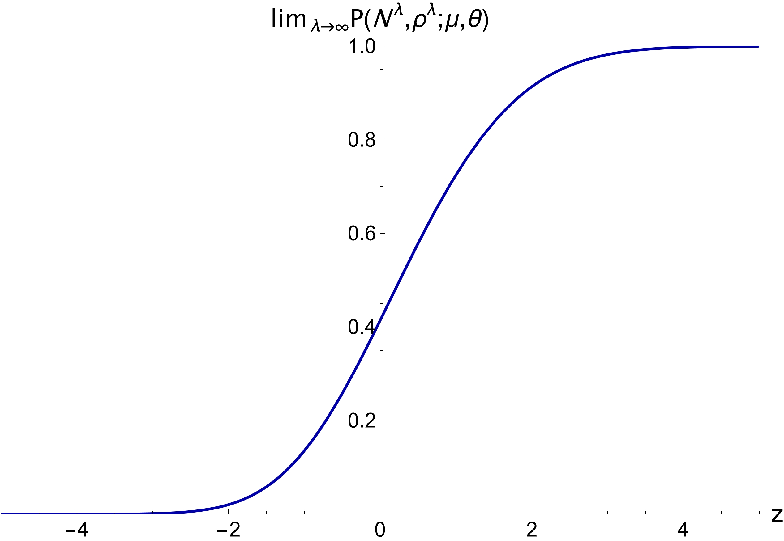
Figure 1: $\lim_{\lambda\to\infty}P(N^{\lambda},\rho^{\lambda};\mu,\theta)$ as a function of $z$ when $\mu=5$ and $\theta=10$.

4 Proof of Theorem 1

The proof leverages the following two auxiliary lemmas, whose proofs are deferred to the end of this section.

Lemma 2

The following are two equivalent integral representations of the reciprocal of $C(N,\rho)$:

(a) $$C(N,\rho)^{-1}=\rho\int_{0}^{\infty}e^{-\rho v}(1+v)^{N-1}vdv.$$ (5)

(b) $$C(N,\rho)^{-1}=1+(N-\rho)\int_{-\infty}^{0}e^{-\rho(e^{-u}-1)-Nu}du.$$ (6)

Lemma 3

Let $\varphi(v;x):=e^{\frac{1}{2}v^{2}-x\left(e^{-\frac{v}{\sqrt{x}}}+\frac{v}{\sqrt{x}}-1\right)}$ for all $v\in\mathbb{R}$ and $x\in\mathbb{R}_{+}$. Then,

$$\varphi(v;x)=\sum_{i=0}^{\infty}a_{i}(v)\cdot x^{-\frac{i}{2}}\quad\forall v\in\mathbb{R}\ \forall x\in\mathbb{R}_{+},$$

where $a_{0}(v)=1$ and $a_{i}(v)$ is a finite polynomial in $v$ for all $i\geq 1$.

We are now ready to prove Theorem 1.

• When $\left|N^{\lambda}-\rho^{\lambda}\right|\in\Theta(\!\sqrt{\lambda})\cup o(\!\sqrt{\lambda})$: Without loss of generality, let $N^{\lambda}=\rho^{\lambda}-z\sqrt{\rho^{\lambda}}+o(\!\sqrt{\rho^{\lambda}})$ for $z\in\mathbb{R}$. Note that $z=\lim_{\lambda\to\infty}\frac{\rho^{\lambda}-N^{\lambda}}{\sqrt{N^{\lambda}}}$.

  From Lemma 2 (b),

  $$C(N^{\lambda},\rho^{\lambda})^{-1}-1=(N^{\lambda}-\rho^{\lambda})\int_{-\infty}^{0}e^{-\rho^{\lambda}(e^{-u}-1)-N^{\lambda}u}du.$$

  Let $v=\!\sqrt{\rho^{\lambda}}\ u$. The above can be equivalently written as

  $$C(N^{\lambda},\rho^{\lambda})^{-1}-1 =\left(\frac{N^{\lambda}-\rho^{\lambda}}{\sqrt{\rho^{\lambda}}}\right)\int_{-\infty}^{0}e^{-\left(\frac{N^{\lambda}-\rho^{\lambda}}{\sqrt{\rho^{\lambda}}}\right)v}e^{-\rho^{\lambda}\left(e^{-\frac{v}{\sqrt{\rho^{\lambda}}}}+\frac{v}{\sqrt{\rho^{\lambda}}}-1\right)}dv$$

  $$=\left(\frac{N^{\lambda}-\rho^{\lambda}}{\sqrt{\rho^{\lambda}}}\right)\int_{-\infty}^{0}e^{-\frac{1}{2}v^{2}-\left(\frac{N^{\lambda}-\rho^{\lambda}}{\sqrt{\rho^{\lambda}}}\right)v}e^{\frac{1}{2}v^{2}-\rho^{\lambda}\left(e^{-\frac{v}{\sqrt{\rho^{\lambda}}}}+\frac{v}{\sqrt{\rho^{\lambda}}}-1\right)}dv$$

  $$=\left(\frac{N^{\lambda}-\rho^{\lambda}}{\sqrt{\rho^{\lambda}}}\right)e^{\frac{1}{2}\left(\frac{N^{\lambda}-\rho^{\lambda}}{\sqrt{\rho^{\lambda}}}\right)^{2}}\int_{-\infty}^{0}e^{-\frac{1}{2}\left(v+\frac{N^{\lambda}-\rho^{\lambda}}{\sqrt{\rho^{\lambda}}}\right)^{2}}\varphi(v;\rho^{\lambda})dv.$$

  Substituting for $\varphi(v;\rho^{\lambda})$ from Lemma 3 and taking the limit as $\lambda\to\infty$, we obtain:

  $$\lim_{\lambda\to\infty}C(N^{\lambda},\rho^{\lambda})^{-1}-1=-z\ \phi(z)^{-1}\lim_{\lambda\to\infty}\sum_{i=0}^{\infty}\left(\rho^{\lambda}\right)^{-\frac{i}{2}}\int_{-\infty}^{0}e^{-\frac{1}{2}\left(v+\frac{N^{\lambda}-\rho^{\lambda}}{\sqrt{\rho^{\lambda}}}\right)^{2}}a_{i}(v)dv.$$

  Finally, noting that every integral within the sum is bounded (since $a_{i}(v)$ are all finite polynomials in $v$) and so, only the first term of the sum would survive in the limit, we obtain:

  $$\lim_{\lambda\to\infty}C(N^{\lambda},\rho^{\lambda})^{-1} =1-z\ \phi(z)^{-1}\lim_{\lambda\to\infty}\int_{-\infty}^{0}e^{-\frac{1}{2}\left(v+\frac{N^{\lambda}-\rho^{\lambda}}{\sqrt{\rho^{\lambda}}}\right)^{2}}dv=1-z\ \phi(z)^{-1}\int_{-\infty}^{0}e^{-\frac{1}{2}(v-z)^{2}}dv$$

  $$=1-z\ \phi(z)^{-1}\int_{z}^{\infty}e^{-\frac{1}{2}t^{2}}dt=1-z\frac{\Phi^{c}(z)}{\phi(z)}=1-\xi(z),$$

  implying that

  $$\lim_{\lambda\to\infty}C(N^{\lambda},\rho^{\lambda})=\big{(}1-\xi(z)\big{)}^{-1}.$$ (7)

  Furthermore, from Lemma 4 in A:

  • If $z>0$, which is the case when $0<\rho^{\lambda}-N^{\lambda}\in\Theta(\!\sqrt{\lambda})$, then $\big{(}1-\xi(z)\big{)}^{-1}\in(1,\infty)$.

  • If $z=0$, which is the case when $\left|N^{\lambda}-\rho^{\lambda}\right|\in o(\!\sqrt{\lambda})$, then $\big{(}1-\xi(z)\big{)}^{-1}=1$.

  • If $z<0$, which is the case when $0<N^{\lambda}-\rho^{\lambda}\in\Theta(\!\sqrt{\lambda})$, then $\big{(}1-\xi(z)\big{)}^{-1}\in(0,1)$.

• When $0<\rho^{\lambda}-N^{\lambda}\in\omega(\!\sqrt{\lambda})$: Let $f(\lambda)=\rho^{\lambda}-N^{\lambda}$. Let $g(\lambda;z)=\rho^{\lambda}-z\sqrt{\rho^{\lambda}}+o(\!\sqrt{\rho^{\lambda}})$ for $z>0$, so that $0<\rho^{\lambda}-g(\lambda;z)\in\Theta(\!\sqrt{\lambda})$.

  By definition of the $\omega$ and $\Theta$ notations, for any $z>0$, there exists $\Lambda(z)$ such that $f(\lambda)\geq\rho^{\lambda}-g(\lambda;z)>0$ for all $\lambda\geq\Lambda(z)$. Since $C(N,\rho)$ is strictly decreasing in $N$ [24, p.8], it follows that, for all $\lambda\geq\Lambda(z)$,

  $$C\left(N^{\lambda},\rho^{\lambda}\right)=C\left(\rho^{\lambda}-f(\lambda),\rho^{\lambda}\right)\geq C\left(g(\lambda;z),\rho^{\lambda}\right),$$

  implying that

  $$\lim_{\lambda\to\infty}C\left(N^{\lambda},\rho^{\lambda}\right)\geq\lim_{\lambda\to\infty}C\left(g(\lambda;z),\rho^{\lambda}\right)=\big{(}1-\xi(z)\big{)}^{-1},$$

  from (7). Since $z>0$ is chosen arbitrarily, we have

  $$\lim_{\lambda\to\infty}C\left(N^{\lambda},\rho^{\lambda}\right)\geq\sup_{z>0}\big{(}1-\xi(z)\big{)}^{-1}=\infty,$$

  from Lemma 4 (b) in A. Therefore,

  $$\lim_{\lambda\rightarrow\infty}C\left(N^{\lambda},\rho^{\lambda}\right)=\infty.$$

• When $0<N^{\lambda}-\rho^{\lambda}\in\omega(\!\sqrt{\lambda})$. Let $f(\lambda)=N^{\lambda}-\rho^{\lambda}$. Let $g(\lambda;z)=\rho^{\lambda}-z\sqrt{\rho^{\lambda}}+o(\!\sqrt{\rho^{\lambda}})$ for $z<0$, so that $0<g(\lambda;z)-\rho^{\lambda}\in\Theta(\!\sqrt{\lambda})$.

  By definition of the $\omega$ and $\Theta$ notations, for any $z<0$, there exists $\Lambda(z)$ such that $f(\lambda)\geq g(\lambda;z)-\rho^{\lambda}>0$ for all $\lambda\geq\Lambda(z)$. Since $C(N,\rho)$ is strictly decreasing in $N$ [24, p.8], it follows that, for all $\lambda\geq\Lambda(z)$,

  $$C\left(N^{\lambda},\rho^{\lambda}\right)=C\left(\rho^{\lambda}+f(\lambda),\rho^{\lambda}\right)\leq C\left(g(\lambda;z),\rho^{\lambda}\right),$$

  implying that

  $$\lim_{\lambda\to\infty}C\left(N^{\lambda},\rho^{\lambda}\right)\leq\lim_{\lambda\to\infty}C\left(g(\lambda;z),\rho^{\lambda}\right)=\big{(}1-\xi(z)\big{)}^{-1},$$

  from (7). Since $z<0$ is chosen arbitrarily, we have

  $$\lim_{\lambda\to\infty}C\left(N^{\lambda},\rho^{\lambda}\right)\leq\inf_{z<0}\big{(}1-\xi(z)\big{)}^{-1}=0,$$

  from Lemma 4 (b). Moreover, it follows from Lemma 2(a) that $C(N,\rho)\geq 0$ for all $N$ and $\rho$. Therefore,

  $$\lim_{\lambda\rightarrow\infty}C\left(N^{\lambda},\rho^{\lambda}\right)=0.$$

  $\blacksquare$

4.1 Proof of Lemma 2

We begin by introducing a closely related performance measure, which is the steady-state probability of blocking in the $M$/$M$/$N$/$N$ queue (also known as the Erlang loss model), where a customer, upon arrival, is immediately lost if all the servers are busy. This quantity is given by the well-known Erlang-B formula [7, p.80]:

$$B\left(N,\rho\right)=\frac{\rho^{N}}{N!}\left(\sum_{i=0}^{N}\frac{\rho^{i}}{i!}\right)^{-1},$$

whose reciprocal admits the following integral representation [15, Theorem 3]:

$$B(N,\rho)^{-1}=\rho\int_{0}^{\infty}e^{-\rho v}(1+v)^{N}dv.$$ (8)

Also, the Erlang-B and Erlang-C formula are related [7, p.92]:

$$C\left(N,\rho\right)=\frac{N\cdot B(N,\rho)}{N-\rho\left(1-B(N,\rho)\right)},$$

which implies that

$$C(N,\rho)^{-1}=1+\left(1-\frac{\rho}{N}\right)\left(B(N,\rho)^{-1}-1\right).$$ (9)

We are now ready to prove Lemma 2. First, the integral appearing on the right hand side of (5) can be written as

$$\rho\int_{0}^{\infty}e^{-\rho v}(1+v)^{N-1}vdv =\rho\int_{0}^{\infty}e^{-\rho v}(1+v)^{N-1}(1+v-1)dv$$

$$=\rho\int_{0}^{\infty}e^{-\rho v}(1+v)^{N}dv-\rho\int_{0}^{\infty}e^{-\rho v}(1+v)^{N-1}dv$$

$$=\rho\int_{0}^{\infty}e^{-\rho v}(1+v)^{N}dv-\frac{\rho}{N}\int_{0}^{\infty}e^{-\rho v}d\left((1+v)^{N}\right)$$

$$=\rho\int_{0}^{\infty}e^{-\rho v}(1+v)^{N}dv-\frac{\rho}{N}\left(e^{-\rho v}(1+v)^{N}\Big{|}_{0}^{\infty}+\rho\int_{0}^{\infty}e^{-\rho v}(1+v)^{N}dv\right)$$

$$=B(N,\rho)^{-1}-\frac{\rho}{N}\left(-1+B(N,\rho)^{-1}\right)=1+\left(1-\frac{\rho}{N}\right)\left(B(N,\rho)^{-1}-1\right)=C(N,\rho)^{-1}$$

from (9), thereby establishing (5).

Next, letting $e^{-u}=1+v$, (8) can be equivalently written as

$$B(N,\rho)^{-1} =\rho\int_{-\infty}^{0}e^{-\rho(e^{-u}-1)-Nu}\cdot e^{-u}du$$

$$=\int_{-\infty}^{0}e^{-\rho(e^{-u}-1)-Nu}\left(\rho e^{-u}-N\right)du+N\int_{-\infty}^{0}e^{-\rho(e^{-u}-1)-Nu}du$$

$$=1+N\int_{-\infty}^{0}e^{-\rho(e^{-u}-1)-Nu}du.$$ (10)

Substituting for $B(N,\rho)^{-1}$ using (4.1) in (9) yields (6). $\blacksquare$

4.2 Proof of Lemma 3

We begin by noting that the Maclaurin series for the exponential function $e^{t}$ converges to the value of the function everywhere on its domain. We use it twice in the proof of Lemma 3; once for each of the two exponential functions in $\varphi(v;x)$. First, the exponent of $\varphi(v;x)$ can be evaluated as:

$$\frac{1}{2}v^{2}-x\,\left(e^{-\frac{v}{\sqrt{x}}}+\frac{v}{\sqrt{x}}-1\right) =\frac{1}{2}v^{2}-x\left(\sum_{i=0}^{\infty}\frac{1}{i!}\left(-\frac{v}{\sqrt{x}}\right)^{i}+\frac{v}{\sqrt{x}}-1\right)=\frac{1}{2}v^{2}-x\sum_{i=2}^{\infty}\frac{1}{i!}\left(-\frac{v}{\sqrt{x}}\right)^{i}$$

$$=-x\sum_{i=3}^{\infty}\frac{1}{i!}\left(-\frac{v}{\sqrt{x}}\right)^{i}=\frac{v^{3}}{\sqrt{x}}\sum_{i=0}^{\infty}\frac{(-1)^{i}}{(i+3)!}\left(\frac{v}{\sqrt{x}}\right)^{i}.$$

Using the Maclaurin series for $e^{t}$ once again, $\varphi(v;x)$ becomes:

$$\varphi(v;x) =\exp\left\{\frac{v^{3}}{\sqrt{x}}\sum_{i=0}^{\infty}\frac{(-1)^{i}}{(i+3)!}\left(\frac{v}{\sqrt{x}}\right)^{i}\right\}=\sum_{j=0}^{\infty}\frac{1}{j!}\left(\frac{v^{3}}{\sqrt{x}}\sum_{i=0}^{\infty}\frac{(-1)^{i}}{(i+3)!}\left(\frac{v}{\sqrt{x}}\right)^{i}\right)^{j}$$

$$=1+\frac{v^{3}}{3!}x^{-\frac{1}{2}}-\left(\frac{v^{4}}{4!}-\frac{v^{6}}{2!(3!)^{2}}\right)x^{-1}+\left(\frac{v^{5}}{5!}-\frac{v^{7}}{3!4!}+\frac{v^{9}}{(3!)^{4}}\right)x^{-\frac{3}{2}}-\left(\frac{v^{6}}{6!}-\frac{9v^{8}}{2!4!5!}+\frac{v^{10}}{2!(3!)^{2}4!}-\frac{v^{12}}{(3!)^{4}4!}\right)x^{-2}+\ldots$$

$$=\sum_{i=0}^{\infty}a_{i}(v)\cdot x^{-\frac{i}{2}},$$

where $a_{0}(v)=1$ and $a_{i}(v)$ is a finite polynomial in $v$ (with degree $3i$) for all $i\geq 1$. $\blacksquare$

Appendix A Properties of the Standard Normal Distribution

In this section, we collect properties of the standard Normal distribution that are used in our proofs. Recall that $\phi(x)=\frac{1}{\sqrt{2\pi}}e^{-\frac{1}{2}x^{2}}$ and $\Phi^{c}(x)=\int_{x}^{\infty}\phi(t)dt$ are the density function and the complementary cumulative distribution function of the standard normal distribution, respectively, and $\xi(x):=x\frac{\Phi^{c}(x)}{\phi(x)}$ for $x\in\mathbb{R}$.

Lemma 4

The function $\xi:\mathbb{R}\mapsto\mathbb{R}$ satisfies the following:

1. $\xi(x)$ is a strictly increasing function of $x$;

2. $\lim_{x\to-\infty}\xi(x)=-\infty$, $\xi(0)=0$, and $\lim_{x\to\infty}\xi(x)=1$.

Proof of Lemma 4. We begin by noting that

$$\phi^{\prime}(x)=\frac{1}{\sqrt{2\pi}}e^{-\frac{x^{2}}{2}}(-x)=-x\phi(x).$$ (11)

Moreover, note that

$$\lim_{x\to\infty}x^{n}\phi(x)=\lim_{x\to\infty}\frac{1}{\sqrt{2\pi}}x^{n}e^{-\frac{x^{2}}{2}}=0,\ \forall n\in\mathbb{N},$$ (12)

since exponential decay dominates polynomial growth. This further implies that

$$\lim_{x\to\infty}x^{n}\Phi^{c}(x)=\lim_{x\to\infty}\frac{\Phi^{c}(x)}{x^{-n}}\overset{(1)}{=}\lim_{x\to\infty}\frac{-\phi(x)}{-nx^{-n-1}}=\lim_{x\to\infty}\frac{x^{n+1}\phi(x)}{n}\overset{(2)}{=}0\quad\forall n\in\mathbb{N},$$ (13)

where (1) follows from L’Hôpital’s rule, and (2) follows from (12).

Proof of (a): Taking the derivative of $\xi(x)$ and using (11) to substitute for $\phi^{\prime}(x)$, we get:

$$\xi^{\prime}(x) =\frac{\phi(x)\left(\Phi^{c}(x)-x\phi(x)\right)-x\Phi^{c}(x)\phi^{\prime}(x)}{\phi(x)^{2}}$$

$$=\frac{\phi(x)\left(\Phi^{c}(x)-x\phi(x)\right)+x^{2}\Phi^{c}(x)\phi(x)}{\phi(x)^{2}}$$

$$=\frac{(1+x^{2})\Phi^{c}(x)-x\phi(x)}{\phi(x)}.$$

Since $\phi(x)>0$ for all $x$, it suffices to show that the numerator of the above display is strictly positive for all $x$. Define $\eta(x):=(1+x^{2})\Phi^{c}(x)-x\phi(x)$. Differentiating $\eta(x)$ once and using (11) to substitute for $\phi^{\prime}(x)$ yields:

$$\eta^{\prime}(x)= 2x\Phi^{c}(x)-(1+x^{2})\phi(x)-\phi(x)-x\phi^{\prime}(x)$$

$$= 2x\Phi^{c}(x)-(1+x^{2})\phi(x)-\phi(x)+x^{2}\phi(x)$$

$$= 2(x\Phi^{c}(x)-\phi(x)).$$

Differentiating $\eta^{\prime}(x)$ once and using (11) to substitute for $\phi^{\prime}(x)$ yields:

$$\eta^{\prime\prime}(x)= 2\left(\Phi^{c}(x)-x\phi(x)-\phi^{\prime}(x)\right)$$

$$= 2\left(\Phi^{c}(x)-x\phi(x)+x\phi(x)\right)=2\Phi^{c}(x)>0,$$

implying that $\eta^{\prime}$ is strictly increasing. Since $\lim_{x\to\infty}\eta^{\prime}(x)=0$ from (13), it follows that $\eta^{\prime}(x)<0$ for all $x$, implying that $\eta$ is strictly decreasing. Finally, since $\lim_{x\to\infty}\eta(x)=0$ from (12) and (13), it follows that $\eta(x)>0$ for all $x$. Hence, $\xi^{\prime}(x)>0$ for all $x$, implying that $\xi(x)$ is a strictly increasing function of $x$.

Proof of (b): It is straightforward to see that

$$\lim_{x\to-\infty}x\frac{\Phi^{c}(x)}{\phi(x)}=-\infty\quad\mbox{ and }\quad\lim_{x\to 0}x\frac{\Phi^{c}(x)}{\phi(x)}=0.$$

Finally, as $x\to\infty$, note that

$$\lim_{x\to\infty}x\frac{\Phi^{c}(x)}{\phi(x)} \overset{(3)}{=}\lim_{x\to\infty}\frac{\Phi^{c}(x)-x\phi(x)}{\phi^{\prime}(x)}\overset{(4)}{=}\lim_{x\to\infty}\frac{\Phi^{c}(x)-x\phi(x)}{-x\phi(x)}=1-\lim_{x\to\infty}\frac{\Phi^{c}(x)}{x\phi(x)}$$

$$\overset{(5)}{=}1-\lim_{x\to\infty}\frac{-\phi(x)}{\phi(x)+x\phi^{\prime}(x)}\overset{(6)}{=}1-\lim_{x\to\infty}\frac{-\phi(x)}{\phi(x)-x^{2}\phi(x)}=1-\lim_{x\to\infty}\frac{1}{x^{2}-1}=1,$$

where (3) and (5) follow from L’Hôpital’s rule, and (4) and (6) follow from (11). $\blacksquare$

Appendix B Proofs from Section 3

B.1 Proof of Lemma 1

The proof of (2) leverages the expressions for the steady-state probabilities of the $M$/$M$/$N$+$M$ queue developed in [4]. From Equations (4.3) and (4.6) in [4], the steady-state probability of having $i$ customers in the system (either being served or waiting in queue), for $i\in\{0,1,2,\ldots,N-1\}$, is given by

$$p_{i}(N,\rho;\mu,\theta)=\frac{\rho^{i}}{i!}\left(\sum_{i=0}^{N-1}\frac{\rho^{i}}{i!}+\frac{\rho^{N-1}}{(N-1)!}\lambda J(N,\rho;\mu,\theta)\right)^{-1}=\frac{\rho^{i}}{i!}\left(\sum_{i=0}^{N-1}\frac{\rho^{i}}{i!}+\frac{\rho^{N}}{N!}(N\mu)J(N,\rho;\mu,\theta)\right)^{-1}.$$

Thus, the steady-state probability of delay is given by

$$P(N,\rho;\mu,\theta)=1-\sum_{i=0}^{N-1}p_{i}(N,\rho;\mu,\theta)=1-\left(\sum_{i=0}^{N-1}\frac{\rho^{i}}{i!}\right)\left(\sum_{i=0}^{N-1}\frac{\rho^{i}}{i!}+\frac{\rho^{N}}{N!}(N\mu)J(N,\rho;\mu,\theta)\right)^{-1},$$

which implies that

$$P(N,\rho;\mu,\theta)=\left(1+\frac{\left(\sum_{i=0}^{N-1}\frac{\rho^{i}}{i!}\right)\Big{/}\frac{\rho^{N}}{N!}}{(N\mu)J(N,\rho;\mu,\theta)}\right)^{-1}=\left(1+\frac{\left(1-\frac{\rho}{N}\right)\left(\sum_{i=0}^{N-1}\frac{\rho^{i}}{i!}\right)\Big{/}\frac{\rho^{N}}{N!}}{\mu(N-\rho)J(N,\rho;\mu,\theta)}\right)^{-1}=\left(1+\frac{C(N,\rho)^{-1}-1}{\mu(N-\rho)J(N,\rho;\mu,\theta)}\right)^{-1},$$

where the last step follows from (1).

Next, for the proof of (4), we first use (3) to write:

$$\mu(N-\rho)J(N,\rho;\mu,\theta)=\mu(N-\rho)\int_{0}^{\infty}e^{\frac{\mu\rho}{\theta}\left(1-e^{-\theta x}\right)-N\mu x}dx.$$

Letting $u=-\theta x$, the above can be equivalently written as

$$\mu(N-\rho)J(N,\rho;\mu,\theta) =\frac{\mu}{\theta}(N-\rho)\int_{-\infty}^{0}e^{\frac{\mu\rho}{\theta}\left(1-e^{u}\right)+\frac{N\mu}{\theta}u}du$$

$$=\int_{-\infty}^{0}e^{\frac{\mu\rho}{\theta}\left(1-e^{u}\right)+\frac{N\mu}{\theta}u}\left(\frac{N\mu}{\theta}-\frac{\mu\rho}{\theta}e^{u}+\frac{\mu\rho}{\theta}(e^{u}-1)\right)du$$

$$=\int_{-\infty}^{0}e^{\frac{\mu\rho}{\theta}\left(1-e^{u}\right)+\frac{N\mu}{\theta}u}\left(\frac{N\mu}{\theta}-\frac{\mu\rho}{\theta}e^{u}\right)du+\frac{\mu\rho}{\theta}\int_{-\infty}^{0}e^{\frac{\mu\rho}{\theta}\left(1-e^{u}\right)+\frac{N\mu}{\theta}u}\left(e^{u}-1\right)du$$

$$=1+\frac{\mu\rho}{\theta}\int_{-\infty}^{0}e^{\frac{\mu\rho}{\theta}\left(1-e^{u}\right)+\frac{N\mu}{\theta}u}\left(e^{u}-1\right)du.$$

Letting $v=1-e^{u}$, the above can be equivalently written as

$$\mu(N-\rho)J(N,\rho;\mu,\theta)=1+\frac{\mu\rho}{\theta}\int_{1}^{0}e^{\frac{\mu\rho}{\theta}v+\frac{N\mu}{\theta}\log(1-v)}(-v)\left(\frac{dv}{1-v}\right)=1+\frac{\mu\rho}{\theta}\int_{0}^{1}e^{\frac{\mu\rho}{\theta}v}(1-v)^{\frac{N\mu}{\theta}-1}vdv.\qquad\;\blacksquare$$

B.2 Proof of Proposition 1

The proof leverages the following auxiliary lemma, whose proof is deferred to B.3..

Lemma 5

If $N^{\lambda}=\rho^{\lambda}-z\sqrt{\rho^{\lambda}}+o(\!\sqrt{\rho^{\lambda}})$ for $z\in\mathbb{R}$, then $\lim_{\lambda\to\infty}\mu(N^{\lambda}-\rho^{\lambda})J(N^{\lambda},\rho^{\lambda};\mu,\theta)=\xi(-\hat{z})$, where $\hat{z}=z\!\sqrt{\frac{\mu}{\theta}}$.

• When $|N^{\lambda}-\rho^{\lambda}|\in\Theta(\!\sqrt{\lambda})\cup o(\!\sqrt{\lambda})$: Without loss of generality, let $N^{\lambda}=\rho^{\lambda}-z\sqrt{\rho^{\lambda}}+o(\!\sqrt{\rho^{\lambda}})$ for $z\in\mathbb{R}$. Note that $z=\lim_{\lambda\to\infty}\frac{\rho^{\lambda}-N^{\lambda}}{\sqrt{N^{\lambda}}}$. From Lemma 1, Theorem 1, and Lemma 5,

  $$\lim_{\lambda\to\infty}P(N^{\lambda},\rho^{\lambda};\mu,\theta)=\lim_{\lambda\to\infty}\left(1+\frac{C(N^{\lambda},\rho^{\lambda})^{-1}-1}{\mu(N^{\lambda}-\rho^{\lambda})J(N^{\lambda},\rho^{\lambda};\mu,\theta)}\right)^{-1}=\left(1-\frac{\xi(z)}{\xi(-\hat{z})}\right)^{-1}.$$ (14)

  Furthermore, from Lemma 4 in A, $\frac{\xi(z)}{\xi(-\hat{z})}$ is strictly increasing in $z$ from $-\infty$ (when $z\to-\infty$) to $-\!\sqrt{\frac{\theta}{\mu}}$ (at $z=0$) to $0$ (when $z\to\infty$), implying the following:

  • If $z>0$, which is the case when $0<\rho^{\lambda}-N^{\lambda}\in\Theta(\!\sqrt{\lambda})$, then $\left(1-\frac{\xi(z)}{\xi(-\hat{z})}\right)^{-1}\in\left(\left(1+\sqrt{\frac{\theta}{\mu}}\right)^{-1},1\right)$.

  • If $z=0$, which is the case when $|N^{\lambda}-\rho^{\lambda}|\in o(\!\sqrt{\lambda})$, then $\left(1-\frac{\xi(z)}{\xi(-\hat{z})}\right)^{-1}=1$.

  • If $z<0$, which is the case when $0<N^{\lambda}-\rho^{\lambda}\in\Theta(\!\sqrt{\lambda})$, then $\left(1-\frac{\xi(z)}{\xi(-\hat{z})}\right)^{-1}\in\left(0,\left(1+\sqrt{\frac{\theta}{\mu}}\right)^{-1}\right)$.

• When $0<\rho^{\lambda}-N^{\lambda}\in\omega(\!\sqrt{\lambda})$: Let $f(\lambda)=\rho^{\lambda}-N^{\lambda}$. Let $g(\lambda;z)=\rho^{\lambda}-z\sqrt{\rho^{\lambda}}+o(\!\sqrt{\rho^{\lambda}})$ for $z>0$, so that $0<\rho^{\lambda}-g(\lambda;z)\in\Theta(\!\sqrt{\lambda})$.

  By definition of the $\omega$ and $\Theta$ notations, for any $z>0$, there exists $\Lambda(z)$ such that $f(\lambda)\geq\rho^{\lambda}-g(\lambda;z)>0$, for all $\lambda\geq\Lambda(z)$. Since $P(N,\rho;\mu,\theta)$, given by Lemma 1, is strictly decreasing in $N$ (recalling that $C(N,\rho)$ is strictly decreasing in $N$ [24, p.8] and the quantity $\mu(N-\rho)J(N,\rho;\mu,\theta)$ is also strictly decreasing in $N$ from (4)), it follows that, for all $\lambda\geq\Lambda(z)$,

  $$P\left(N^{\lambda},\rho^{\lambda};\mu,\theta\right)=P\left(\rho^{\lambda}-f(\lambda),\rho^{\lambda};\mu,\theta\right)\geq P\left(g(\lambda;z),\rho^{\lambda};\mu,\theta\right),$$

  implying that

  $$\lim_{\lambda\to\infty}P\left(N^{\lambda},\rho^{\lambda};\mu,\theta\right)\geq\lim_{\lambda\to\infty}P\left(g(\lambda;z),\rho^{\lambda};\mu,\theta\right)=\left(1-\frac{\xi(z)}{\xi(-\hat{z})}\right)^{-1},$$

  from (14). Since $z>0$ is chosen arbitrarily, we have

  $$\lim_{\lambda\to\infty}P\left(N^{\lambda},\rho^{\lambda};\mu,\theta\right)\geq\sup_{z>0}\left(1-\frac{\xi(z)}{\xi(-\hat{z})}\right)^{-1}=1,$$

  from the preceding discussion. Therefore,

  $$\lim_{\lambda\to\infty}P(N^{\lambda},\rho^{\lambda};\mu,\theta)=1.$$

• When $0<N^{\lambda}-\rho^{\lambda}\in\omega(\!\sqrt{\lambda})$. Let $f(\lambda)=N^{\lambda}-\rho^{\lambda}$. Let $g(\lambda;z)=\rho^{\lambda}-z\sqrt{\rho^{\lambda}}+o(\!\sqrt{\rho^{\lambda}})$ for $z<0$, so that $0<g(\lambda;z)-\rho^{\lambda}\in\Theta(\!\sqrt{\lambda})$.

  By definition of the $\omega$ and $\Theta$ notations, for any $z<0$, there exists $\Lambda(z)$ such that $f(\lambda)\geq g(\lambda;z)-\rho^{\lambda}>0$, for all $\lambda\geq\Lambda(z)$. Since $P(N,\rho;\mu,\theta)$, given by Lemma 1, is strictly decreasing in $N$ (recalling that $C(N,\rho)$ is strictly decreasing in $N$ [24, p.8] and the quantity $\mu(N-\rho)J(N,\rho;\mu,\theta)$ is also strictly decreasing in $N$ from (4)), it follows that, for all $\lambda\geq\Lambda(z)$,

  $$P\left(N^{\lambda},\rho^{\lambda};\mu,\theta\right)=P\left(\rho^{\lambda}+f(\lambda),\rho^{\lambda};\mu,\theta\right)\leq P\left(g(\lambda;z),\rho^{\lambda};\mu,\theta\right),$$

  implying that

  $$\lim_{\lambda\to\infty}P\left(N^{\lambda},\rho^{\lambda};\mu,\theta\right)\leq\lim_{\lambda\to\infty}P\left(g(\lambda;z),\rho^{\lambda};\mu,\theta\right)=\left(1-\frac{\xi(z)}{\xi(-\hat{z})}\right)^{-1},$$

  from (14). Since $z<0$ is chosen arbitrarily, we have

  $$\lim_{\lambda\to\infty}P\left(N^{\lambda},\rho^{\lambda};\mu,\theta\right)\leq\inf_{z<0}\left(1-\frac{\xi(z)}{\xi(-\hat{z})}\right)^{-1}=0,$$

  from the preceding discussion. Therefore,

  $$\lim_{\lambda\to\infty}P(N^{\lambda},\rho^{\lambda};\mu,\theta)=0.$$

  $\blacksquare$

B.3 Proof of Lemma 5

From (3), we have:

$$\mu(N^{\lambda}-\rho^{\lambda})J(N^{\lambda},\rho^{\lambda};\mu,\theta)=\mu(N^{\lambda}-\rho^{\lambda})\int_{0}^{\infty}e^{\frac{\mu\rho^{\lambda}}{\theta}\left(1-e^{-\theta x}\right)-N^{\lambda}\mu x}dx.$$

Letting $u=\theta x$, the above can be equivalently written as

$$\mu(N^{\lambda}-\rho^{\lambda})J(N^{\lambda},\rho^{\lambda};\mu,\theta)=\frac{\mu}{\theta}(N^{\lambda}-\rho^{\lambda})\int_{0}^{\infty}e^{\frac{\mu\rho^{\lambda}}{\theta}\left(1-e^{-u}\right)-\frac{N^{\lambda}\mu}{\theta}u}du.$$

Let $\hat{N}^{\lambda}=\frac{\mu}{\theta}N^{\lambda}$ and $\hat{\rho}^{\lambda}=\frac{\mu}{\theta}\rho^{\lambda}$ for all $\lambda>0$, and $\hat{z}=z\!\sqrt{\frac{\mu}{\theta}}$. Then, $N^{\lambda}=\rho^{\lambda}-z\sqrt{\rho^{\lambda}}+o(\!\sqrt{\rho^{\lambda}})$ is equivalent to $\hat{N}^{\lambda}=\hat{\rho}^{\lambda}-\hat{z}\sqrt{\hat{\rho}^{\lambda}}+o(\!\sqrt{\hat{\rho}^{\lambda}})$ and the above can be equivalently written as

$$\mu(N^{\lambda}-\rho^{\lambda})J(N^{\lambda},\rho^{\lambda};\mu,\theta)=(\hat{N}^{\lambda}-\hat{\rho}^{\lambda})\int_{0}^{\infty}e^{-\hat{\rho}^{\lambda}\left(e^{-u}-1\right)-\hat{N}^{\lambda}u}du.$$

Let $v=\!\sqrt{\hat{\rho}^{\lambda}}\ u$. The above can be equivalently written as

$$\mu(N^{\lambda}-\rho^{\lambda})J(N^{\lambda},\rho^{\lambda};\mu,\theta) =\left(\frac{\hat{N}^{\lambda}-\hat{\rho}^{\lambda}}{\sqrt{\hat{\rho}^{\lambda}}}\right)\int_{0}^{\infty}e^{-\left(\frac{\hat{N}^{\lambda}-\hat{\rho}^{\lambda}}{\sqrt{\hat{\rho}^{\lambda}}}\right)v}e^{-\hat{\rho}^{\lambda}\left(e^{-\frac{v}{\sqrt{\hat{\rho}^{\lambda}}}}+\frac{v}{\sqrt{\hat{\rho}^{\lambda}}}-1\right)}dv$$

$$=\left(\frac{N^{\lambda}-\hat{\rho}^{\lambda}}{\sqrt{\hat{\rho}^{\lambda}}}\right)\int_{0}^{\infty}e^{-\frac{1}{2}v^{2}-\left(\frac{\hat{N}^{\lambda}-\hat{\rho}^{\lambda}}{\sqrt{\hat{\rho}^{\lambda}}}\right)v}e^{\frac{1}{2}v^{2}-\hat{\rho}^{\lambda}\left(e^{-\frac{v}{\sqrt{\hat{\rho}^{\lambda}}}}+\frac{v}{\sqrt{\hat{\rho}^{\lambda}}}-1\right)}dv$$

$$=\left(\frac{\hat{N}^{\lambda}-\hat{\rho}^{\lambda}}{\sqrt{\hat{\rho}^{\lambda}}}\right)e^{\frac{1}{2}\left(\frac{\hat{N}^{\lambda}-\hat{\rho}^{\lambda}}{\sqrt{\hat{\rho}^{\lambda}}}\right)^{2}}\int_{0}^{\infty}e^{-\frac{1}{2}\left(v+\frac{\hat{N}^{\lambda}-\hat{\rho}^{\lambda}}{\sqrt{\hat{\rho}^{\lambda}}}\right)^{2}}\varphi(v;\hat{\rho}^{\lambda})dv.$$

Substituting for $\varphi(v;\hat{\rho}^{\lambda})$ from Lemma 3 and taking the limit as $\lambda\to\infty$, we obtain:

$$\lim_{\lambda\to\infty}\mu(N^{\lambda}-\rho^{\lambda})J(N^{\lambda},\rho^{\lambda};\mu,\theta)=-\hat{z}\ \phi(-\hat{z})^{-1}\lim_{\lambda\to\infty}\sum_{i=0}^{\infty}\left(\hat{\rho}^{\lambda}\right)^{-\frac{i}{2}}\int_{0}^{\infty}e^{-\frac{1}{2}\left(v+\frac{\hat{N}^{\lambda}-\hat{\rho}^{\lambda}}{\sqrt{\hat{\rho}^{\lambda}}}\right)^{2}}a_{i}(v)dv,$$

recalling that $\hat{z}=\lim_{\lambda\to\infty}\frac{\hat{\rho}^{\lambda}-\hat{N}^{\lambda}}{\sqrt{\hat{\rho}^{\lambda}}}$. Finally, noting that every integral within the sum is bounded (since $a_{i}(v)$ are all finite polynomials in $v$) and so, only the first term of the sum would survive in the limit, we obtain:

$$\lim_{\lambda\to\infty}\mu(N^{\lambda}-\rho^{\lambda})J(N^{\lambda},\rho^{\lambda};\mu,\theta) =-\hat{z}\ \phi(-\hat{z})^{-1}\lim_{\lambda\to\infty}\int_{0}^{\infty}e^{-\frac{1}{2}\left(v+\frac{\hat{N}^{\lambda}-\hat{\rho}^{\lambda}}{\sqrt{\hat{\rho}^{\lambda}}}\right)^{2}}dv=-\hat{z}\ \phi(-\hat{z})^{-1}\int_{0}^{\infty}e^{-\frac{1}{2}(v-\hat{z})^{2}}dv$$

$$=-\hat{z}\ \phi(-\hat{z})^{-1}\int_{-\hat{z}}^{\infty}e^{-\frac{1}{2}t^{2}}dt=-\hat{z}\frac{\Phi^{c}(-\hat{z})}{\phi(-\hat{z})}=\xi(-\hat{z}).\qquad\qquad\qquad\qquad\qquad\quad\;\;\,\blacksquare$$

References

• Aksin et al. [2007] Aksin, Zeynep, Mor Armony, Vijay Mehrotra. 2007. The modern call center: A multi-disciplinary perspective on operations management research. Production and Operations Management 16(6) 665–688.
• Anick et al. [1982] Anick, David, Debasis Mitra, Man M Sondhi. 1982. Stochastic theory of a data-handling system with multiple sources. Bell System Technical Journal 61(8) 1871–1894.
• Armony et al. [2015] Armony, Mor, Shlomo Israelit, Avishai Mandelbaum, Yariv N Marmor, Yulia Tseytlin, Galit B Yom-Tov. 2015. On patient flow in hospitals: A data-based queueing-science perspective. Stochastic Systems 5(1) 146–194.
• Baccelli and Hebuterne [1981] Baccelli, Francois, Gerard Hebuterne. 1981. On queues with impatient customers. Ph.D. thesis, INRIA.
• Borst et al. [2004] Borst, Sem, Avi Mandelbaum, Martin I Reiman. 2004. Dimensioning large call centers. Operations Research 52(1) 17–34.
• Brown et al. [2005] Brown, Lawrence, Noah Gans, Avishai Mandelbaum, Anat Sakov, Haipeng Shen, Sergey Zeltyn, Linda Zhao. 2005. Statistical analysis of a telephone call center: A queueing-science perspective. Journal of the American Statistical Association 100(469) 36–50.
• Cooper [1981] Cooper, R. B. 1981. Introduction to Queueing Theory. North Holland, New York.
• Erlang [1917] Erlang, Agner Krarup. 1917. Solution of some problems in the theory of probabilities of significance in automatic telephone exchanges. Post Office Electrical Engineer’s Journal 10 189–197.
• Gans et al. [2003] Gans, Noah, Ger Koole, Avishai Mandelbaum. 2003. Telephone call centers: Tutorial, review, and research prospects. Manufacturing & Service Operations Management 5(2) 79–141.
• Garnett et al. [2002] Garnett, Ofer, Avishai Mandelbaum, Martin Reiman. 2002. Designing a call center with impatient customers. Manufacturing & Service Operations Management 4(3) 208–227.
• Gopalakrishnan et al. [2016] Gopalakrishnan, Ragavendran, Sherwin Doroudi, Amy R Ward, Adam Wierman. 2016. Routing and staffing when servers are strategic. Operations Research 64(4) 1033–1050.
• Green et al. [2007] Green, Linda V, Sergei Savin, Mark Murray. 2007. Providing timely access to care: What is the right patient panel size? The Joint Commission Journal on Quality and Patient Safety 33(4) 211–218.
• Halfin and Whitt [1981] Halfin, Shlomo, Ward Whitt. 1981. Heavy-traffic limits for queues with many exponential servers. Operations Research 29(3) 567–588.
• Harel [1988] Harel, Arie. 1988. Sharp bounds and simple approximations for the Erlang delay and loss formulas. Management Science 34(8) 959–972.
• Jagerman [1974] Jagerman, David L. 1974. Some properties of the Erlang loss function. Bell System Technical Journal 53(3) 525–551.
• Kelly [1985] Kelly, Frank P. 1985. Stochastic models of computer communication systems. Journal of the Royal Statistical Society: Series B (Methodological) 47(3) 379–395.
• Kim and Randhawa [2018] Kim, Jeunghyun, Ramandeep S Randhawa. 2018. The value of dynamic pricing in large queueing systems. Operations Research 66(2) 409–425.
• Kolesar and Green [1998] Kolesar, Peter J, Linda V Green. 1998. Insights on service system design from a normal approximation to Erlang’s delay formula. Production and Operations Management 7(3) 282–293.
• Mandelbaum and Zeltyn [2009] Mandelbaum, Avishai, Sergey Zeltyn. 2009. Staffing many-server queues with impatient customers: Constraint satisfaction in call centers. Operations Research 57(5) 1189–1205.
• Nair et al. [2016] Nair, Jayakrishnan, Adam Wierman, Bert Zwart. 2016. Provisioning of large-scale systems: The interplay between network effects and strategic behavior in the user base. Management Science 62(6) 1830–1841.
• Palm [1943] Palm, Conny. 1943. Intensitatsschwankungen im fernsprechverker. Ericsson Technics .
• Turpin Jr [Forthcoming] Turpin Jr, Lonnie. Forthcoming. Service staffing with delay probabilities. Operations Research Letters .
• van Leeuwaarden et al. [2019] van Leeuwaarden, Johan SH, Britt WJ Mathijsen, Bert Zwart. 2019. Economies-of-scale in many-server queueing systems: Tutorial and partial review of the QED Halfin–Whitt heavy-traffic regime. SIAM Review 61(3) 403–440.
• Whitt [2002] Whitt, W. 2002. IEOR 6707: Advanced topics in queueing theory: Focus on customer contact centers. Homework 1e Solutions, see http://www.columbia.edu/~ww2040/ErlangBandCFormulas.pdf.
• Whitt [1999] Whitt, Ward. 1999. Dynamic staffing in a telephone call center aiming to immediately answer all calls. Operations Research Letters 24(5) 205–212.
• Yom-Tov [2010] Yom-Tov, Galit Bracha. 2010. Queues in hospitals: Queueing networks with reentering customers in the QED regime. Ph.D. thesis, The Technion-Israel Institute of Technology.
• Zeltyn and Mandelbaum [2005] Zeltyn, Sergey, Avishai Mandelbaum. 2005. Call centers with impatient customers: Many-server asymptotics of the M/M/N+G queue. Queueing Systems 51(3-4) 361–402.
• Zhan and Ward [2019] Zhan, Dongyuan, Amy R Ward. 2019. Staffing, routing, and payment to trade off speed and quality in large service systems. Operations Research 67(6) 1738–1751.
• Zhong et al. [2023] Zhong, Yueyang, Raga Gopalakrishnan, Amy Ward. 2023. Behavior-aware queueing: The finite-buffer setting with many strategic servers. Operations Research .
• Zhong et al. [2022] Zhong, Yueyang, Amy R Ward, Amber L Puha. 2022. Asymptotically optimal idling in the GI/GI/N+GI queue. Operations Research Letters 50(3) 362–369.