On Pitfalls of RemOve-And-Retrain:
Data Processing Inequality Perspective

Abstract

Approaches for appraising feature importance approximations, alternatively referred to as attribution methods, have been established across an extensive array of contexts. The development of resilient techniques for performance benchmarking constitutes a critical concern in the sphere of explainable deep learning. This study scrutinizes the dependability of the RemOve-And-Retrain (ROAR) procedure, which is prevalently employed for gauging the performance of feature importance estimates. The insights gleaned from our theoretical foundation and empirical investigations reveal that attributions containing lesser information about the decision function may yield superior results in ROAR benchmarks, contradicting the original intent of ROAR. This occurrence is similarly observed in the recently introduced variant RemOve-And-Debias (ROAD), and we posit a persistent pattern of blurriness bias in ROAR attribution metrics. Our findings serve as a warning against indiscriminate use on ROAR metrics. The code is available as open source.

1 Introduction

The estimation of feature importance, also known as attribution or post-hoc model explanation, aims to accurately measure the contribution of each feature to the final decision made by neural networks. A range of techniques have been proposed for this purpose, including input-gradient Baehrens et al. (2010); Simonyan et al. (2014), Integrated Gradient Sundararajan et al. (2017), Grad-CAM Selvaraju et al. (2017), DeepLIFT Shrikumar et al. (2017), SmoothGrad Smilkov et al. (2017), and VarGrad Hooker et al. (2019). Despite significant advances in this field, the estimation of feature importance for neural network decisions remains an open research area Samek et al. (2021).

Assessing the accuracy of feature importance estimates is a challenging problem due to the lack of a ground truth for model interpretability. Despite this, researchers have made significant efforts to develop quantitative evaluation methods for attribution techniques, including Samek et al. (2016); Dabkowski and Gal (2017); Adebayo et al. (2018b); Hooker et al. (2019); Adebayo et al. (2020). However, selecting the most effective evaluation metric that accurately reflects the performance of attribution methods remains a contentious issue in the field.

One influential method for evaluating a range of feature importance estimates is the "Remove-And-Retrain" (ROAR) method proposed in Hooker et al. (2019). This method has been widely adopted in the evaluation of newly proposed attribution methods Schramowski et al. (2020); Liang et al. (2020); Kim et al. (2019a); Yang et al. (2020); O’Shaughnessy et al. (2020); Khakzar et al. (2021); Hartley et al. (2021); Chefer et al. (2021); Ismail et al. (2021); Meng et al. (2022), as well as in studies related to the development of novel evaluation metrics Bhatt et al. (2020); Ismail et al. (2020); DeYoung et al. (2020); Zhang et al. (2021). In addition, Kim et al. (2019b) extended the use of ROAR to measure the fixed attribution interpretability of various model functions $f(\cdot;\theta)$. It is clear that the ROAR evaluation metric has had a significant impact on the field of machine learning interpretability.

In this study, we question the widespread adoption of the RemOve-And-Retrain (ROAR) metric. We draw attention to the problematic behavior of the ROAR evaluation metric and provide both theoretical rationale and empirical evidence to support our objections. Our significant finding is that attributions that naturally possess reduced information about the decision function can lead to enhanced performance on ROAR metrics. Our key contributions are as follows:

• We demonstrate that the attribution of an explainer which never has more information about the model can result in better performance in the ROAR metric.

• To support our claim, we provide a theoretical rationale of ROAR’s assumptions, a comprehensive dependency graph for the data generation process, and extensive experiments on real-world datasets.

• We also show that there is a bias towards attribution bluriness in the ROAR metric, which is related to the unfavorable behavior of the ROAR metric.

2 Preliminaries

2.1 Notions and Notations

Let $\mathcal{X}$ and $\mathcal{Y}$ denote the input space and class label space, respectively. We consider a $C$-class multi-class pre-softmax classifier $f(x;\theta):\mathcal{X}\times\Theta\rightarrow\mathbb{R}^{C}$ with parameters $\theta$, and define $\mathcal{F}$ as the set of all possible functions $f(\cdot;\theta):\mathcal{X}\rightarrow\mathbb{R}^{C}$ for a given $\theta$. A feature importance measure (or explainer), also referred to as an attribution method Ancona et al. (2018), is a function $e(x,f(\cdot;\theta),y):\mathcal{X}\times\mathcal{F}\times\mathcal{Y}\rightarrow\tilde{\mathcal{X}}$ that identifies which input features are important in determining a class decision $y\in\mathcal{Y}$ given an input $x$ and a function $f(\cdot;\theta)$ Lundberg and Lee (2017); Hooker et al. (2019). As an example, input-gradient Baehrens et al. (2010); Simonyan et al. (2014), a widely recognized basic feature importance measure methodology, is defined as $e(x,f(\cdot;\theta),y)=\frac{\partial{f(\text{x};\theta)}y}{\partial\text{x}}\Bigr{\rvert}_{\text{x}=x}$, where ${f(\text{x};\theta)}_{y}$ is the $y$-th indexed value of $f(\text{x};\theta)$. In this paper, the output of the explainer is referred to as an "attribution map." For consistency, variables are denoted using uppercase letters, while functions or values are denoted using lowercase letters, with some exceptions.

Input : $f(x;\theta):\mathcal{X}\times\Theta\mapsto\mathbb{R}^{c}$, $c$-classes multi-class pre-softmax classifier with parameters $\theta$.
$e(x,f(\cdot;\theta),y):\mathcal{X}\times\mathcal{F}\times\mathcal{Y}\mapsto\tilde{\mathcal{X}}$, feature importance estimate.
$k(a):\tilde{\mathcal{X}}\mapsto\tilde{\mathcal{X}}$, post-processing of attribution.
$D_{train}$ & $D_{test}$, training dataset and test dataset.
$T$, list of drop rates for feature importance estimate.

Output : $V$, dictionary with threshold as key and corresponding ROAR measure as value.

1 $\hat{\theta}\leftarrow\operatorname*{arg\,min}_{\theta\in\Theta}\mathbb{E}_{(x,y)\in D_{train}}[L(f(x;\theta),y)];$ and $V\leftarrow\{\}$;

2 $A_{train}\leftarrow[e(x,f(\cdot;\hat{\theta}),\operatorname*{arg\,min}_{i\in C}f_{i}(x;\hat{\theta}))\text{ for }(x,y)\text{ in }D_{train}]$;

3 $A_{test}\leftarrow[e(x,f(\cdot;\hat{\theta}),\operatorname*{arg\,min}_{i\in C}f_{i}(x;\hat{\theta}))\text{ for }(x,y)\text{ in }D_{test}]$;

4 $A_{train}\leftarrow[k(a)\text{ for }a\text{ in }A_{train}]$;

5 $A_{test}\leftarrow[k(a)\text{ for }a\text{ in }A_{test}]$;

6

7for $t$ in $T$ do

8       $M_{train}\leftarrow[\{a>Percentile(a,t)\}\text{ for }a\text{ in }A_{train}]$;

9       $M_{test}\leftarrow[\{a>Percentile(a,t)\}\text{ for }a\text{ in }A_{test}]$;

10       $D^{\prime}_{train}\leftarrow[(1-m)\odot x,y)\text{ for }((x,y),m)\text{ in }\text{zip}(D_{train},M_{train})$;

11       $D^{\prime}_{test}\leftarrow[(1-m)\odot x,y)\text{ for }((x,y),m)\text{ in }\text{zip}(D_{test},M_{test})$;

12       $\hat{\theta}_{new}\leftarrow\operatorname*{arg\,min}_{\theta\in\Theta}\mathbb{E}_{(x^{\prime},y)\in D^{\prime}_{train}}[L(f(x^{\prime}),y)]$;

13       $Acc\leftarrow\mathbb{E}_{(x^{\prime},y)\in D^{\prime}_{test}}[\mathds{1}_{\operatorname*{arg\,min}_{i\in C}f_{i}(x^{\prime};\hat{\theta}_{new})=y}]$;

14       $V\text{.update}(\{t:Acc\})$;

15      

16 end for

Algorithm 1 RemOve-And-Retrain (ROAR) with our modification

2.2 RemOve-And-Retrain (ROAR)

To make our work self-contained, we present a brief introduction here Hooker et al. (2019). Algorithm 1 outlines the pseudo-code for the ROAR procedure in Python style. The proposal of ROAR was motivated by the limitations of existing modification-based evaluation methods Bach et al. (2015); Samek et al. (2016). At the time, the dominant approach for modification-based evaluation was a type of sequential procedure that only used the test dataset $D_{test}$. This approach involves applying attribution methods (line 3), sorting feature importance estimates and modifying features with high attribution values (lines 8 and 10), and measuring the performance drops of the trained classifier (lines 12 and 13). It should be noted that, in this case, $\hat{\theta}_{new}\leftarrow\hat{\theta}$ because the parameters of the classifier are never changed. However, Dabkowski and Gal (2017); Fong and Vedaldi (2017) have pointed out that it is difficult to determine whether the performance drops are due to the significance of the feature importance estimates or to the out-of-distribution nature of the input samples.

To address the issue of a distribution gap between training data and testing data, the ROAR approach employs a re-training strategy. This involves applying data processing techniques to the training data, $D_{train}$, in a similar manner to how they are applied to the testing data in the previously described modification-based evaluation. Specifically, after sorting the attribution for each instance based on feature importance (Line 1), a new training dataset, $D^{\prime}_{train}$, is created by dropping a certain percentage of features (as determined by the parameter $t$, see Line 1). The model is then re-trained on this synthesized training dataset to produce new parameters, $\hat{\theta}_{new}$ (Line 1). These new parameters are used to evaluate model performance, rather than the original parameters, $\hat{\theta}$, in order to alleviate the distribution mismatch between the training and testing datasets (Line 1).

The recent work Rong et al. (2022) has demonstrated that mutual information (MI) between data variable and class variable can be utilized as a surrogate for attainable accuracy in pixel removal strategies that involve retraining, as higher MI generally leads to higher accuracy Hellman and Raviv (1970); Schramowski et al. (2020). In the ROAR approach, MI between the modified data variable and the class variable is particularly important, as it determines the obtainable accuracy. In this context, low MI between the modified data variable and the class variable is desirable, as it results in a decrease in accuracy and improved benchmarking results.

3 Sanity Check in view of DPI

3.1 Sketch of Our Argument

In this study, we build upon the following theorem, mentioned in the previous Section 2.2:

Theorem 3.1 (Rong et al. (2022), stated informally).

The better ROAR benchmark Hooker et al. (2019) indicates a lower value of $I(X^{\prime};Y)$,

where $I(X^{\prime};Y)$ represents mutual information between random variables $X^{\prime}$ and $Y$. The ROAR metric assumes that the output of the explainer $e$ for the function $f$’s decision on $x$ can be fully represented by the modified input $\mathbf{x^{\prime}}$ for the estimation of $I(X^{\prime};Y)$. This assumption raises questions, as it has not been rigorously validated. To ensure the validity of the ROAR metric, it is crucial to perform a sanity check to confirm that the measurement of $I(X^{\prime};Y)$ accurately reflects the information content about the explainer and model.

To examine the underlying assumption, we examine the dependency graph (or structural causal model) for the process of generating $X^{\prime}$. 1 represents a structural causal model for the generation of modified data variables ${X}^{\prime}$ or $\widetilde{X}^{\prime}$. The black nodes and associated random variable names are from the existing ROAR framework, while the blue nodes and variables are newly introduced to demonstrate the focus of our work. Each node represents a distinct variable, with $X$ representing the input data, $E_{F}$ the explainer-based decision function, $A$ the attribution, $X^{\prime}$ the modified input data derived from $X$ and $A$, $\widetilde{A}$ the modified attribution generated by $k(\cdot)$, and $\widetilde{X}^{\prime}$ the modified input data derived from $X$ and $\widetilde{A}$. For simplicity, in the text we omit the subscript $F$ as the decision function is considered fixed. The attribution variable $A$ serves as a collider between data $X$ and explainer $E$. At the same time, $X$ is a common cause of both $A$ and ${X}^{\prime}$, thereby leading to a spurious correlation among these variables that can hinder the accurate recognition of the causal effect. As a result, it remains unclear to what extent $E$ and $F$ influence the ROAR benchmarks (measuring $I(X^{\prime};Y)$) through the observation of ${X}^{\prime}$.

The goal of feature importance estimation is to assess the effect of the explainer $E$ while controlling for the data $X$ and the decision function. To achieve this, $E$ can be augmented with $\widetilde{E}$, which allows observing the treatment effect of ${X}^{\prime}$ when $X$ is fixed. The process of obtaining $\widetilde{E}$ involves applying post-processing $k$ to the result of $E$, with $k$ only relying on the outcome of $E$ and not on $X$ or the decision function. Instead of using $\widetilde{E}$, we assume $E$ and $k$ can be separated, with $k$ being applied to the attribution $A$ and the result referred to as $\widetilde{A}$, i.e. $\widetilde{a}=k(a)$. Finally, $\widetilde{X}^{\prime}$ is calculated as the modification of $X$ with $\widetilde{m}=\{\widetilde{a}>Percentile(\widetilde{a},t)\}$, as $\widetilde{x}^{\prime}=(1-\widetilde{m})\odot x$. Note that $m=\{a>Percentile(a,t)\}$ and $x^{\prime}=(1-m)\odot x$.

In the context of our data processing framework, it is noteworthy to mention that the Data Processing Inequality (DPI) holds when $X$ is controlled, as established by the Markov chain $E\rightarrow A\rightarrow\widetilde{A}$. This result can be found in Thomas and Joy (2006) as stated in the following theorem:

Theorem 3.2 (Data Processing Inequality).

For the Structural Causal Model represented in Fig. 1, it holds that $I(E;A|X=x)\geq I(E;\widetilde{A}|X)$.

This theorem asserts that when $X$ is controlled, $A$ cannot contain less information about $E$ than $\widetilde{A}$. As a result, ${X}^{\prime}$ cannot have less information about $E$ than $\widetilde{X}^{\prime}$. This is due to the dependence of ${X}^{\prime}$ on $X$ and $A$, and the dependence of $\widetilde{{X}}^{\prime}$ on $X$ and $\widetilde{A}$. It is worth noting that the control (or conditioning) by variable $X$ ensures that $A$ and $\widetilde{A}$ result in processing on the exact same data instance.

Our main objective in this study is to identify existence of the post-processing $k$ that results in improved ROAR benchmarks. It confirms the following conjecture, which is based on Theorem 3.1 and the DPI:

Conjecture 3.3.

There may exist a post-processing function $k$ such that $I({X}^{\prime};Y)>I(\widetilde{X}^{\prime};Y)$, while also satisfying $I(E;{X}^{\prime}|X)\geq I(E;\widetilde{X}^{\prime}|X)$.

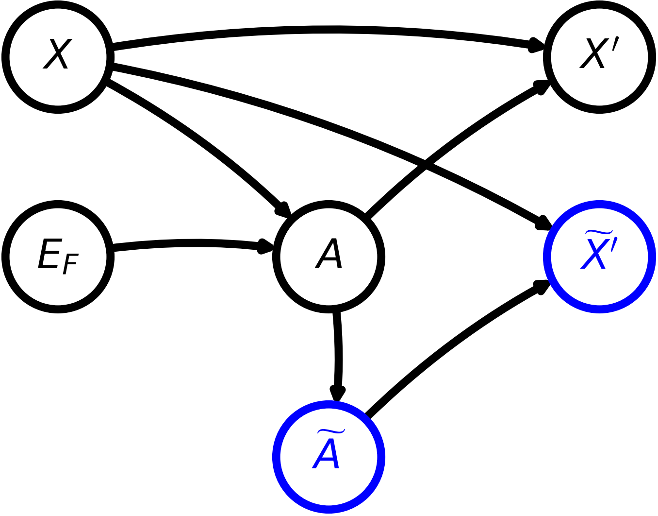
Figure 1: A structural causal model for the generation of modified data variables.

		Plain	Max-pool	Gaussian
	$\widetilde{m}$
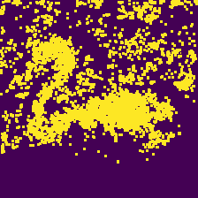
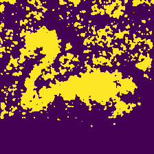
	$\widetilde{x}^{\prime}$

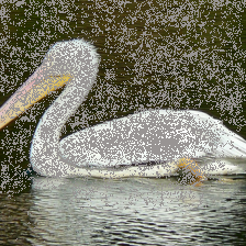
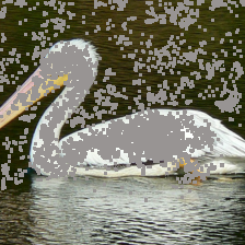
Figure 2: Model/Data-agnostic attribution post-processings. The term ’Plain’ indicates that no post-processing has been applied, i.e., $k(a)=a$. The leftmost image represents the original input image $x$. The feature importance measure used in this illustration is the input-gradient method.

The conjecture suggests that there is a specific kind of post-processing improving ROAR benchmark scores, but at the cost of reduced information about the explainer and the decision function. It implies that the attribution of an explainer which never has more information about the model can result in better performance in the ROAR metric. This behavior contradicts the original intentions of the ROAR protocol, raising concerns about the reliability of the ROAR metric as an evaluation tool for feature importance estimates.

3.2 Instantiation of Post-processing

We presents two simple forms of post-processing $k(\cdot)$: the Gaussian filter and the max-pooling filter. These post-processing methods are applied to the attribution map $a$ to demonstrate their effect on reducing the ROAR measure (as described in lines 1 and 1 in Algorithm 1). The operations are illustrated in Figure 2. It is important to note that these degradation processes are conducted using only the attribution map $a$ and do not require any additional information such as the input data, the methodology used to estimate feature importance, or the model. The results presented in Section 4.2 show that these post-processings agnostic to the model and function can effectively improve the ROAR and ROAD metric.

Rationale of Choice

The choice of post-processing method $k$ in Conjecture 3.3 is motivated by a comparison of two random baselines. The first baseline, referred to as "PixelRandom," involves randomly selecting pixel positions to be erased, covering $t$ percent of the entire possible mask area. The second baseline, "BlockRandom," involves randomly selecting a single rectangle mask to cover $t$ percent of the mask area. As demonstrated in Figure 3, both baselines are agnostic to the model and data.

However, the results of the ROAR measure appear to be biased towards BlockRandom, as indicated in Table 1. This is due to the difference in information loss resulting from the image’s feature information, including pixel value and spatial characteristics. The gradient of a natural image is typically sparse compared to the total image space, leading to pixels with similar values to adjacent pixels. This observation also aligns with the concept of total variation prior Rudin et al. (1992) in image restoration. The information loss caused by BlockRandom is greater than that of PixelRandom, even when equal proportions of pixel values are dropped.

Figure 3: (a) Input Image, (b) PixelRandom, and (c) BlockRandom. Examples of PixelRandom and BlockRandom.

	10%	30%	50%	70%	90%
PixelRandom	0.7556	0.7269	0.7099	0.6772	0.6195
BlockRandom	0.6586	0.4384	0.2815	0.1705	0.0533

Table 1: The results of the ROAR method applied to the CUB-200 dataset using PixelRandom and BlockRandom. Each column represents the attribution drop rate $t\in T$. The specifics of the experimental setup are outlined in Section 3.2.

Based on these observations, we hypothesized that using a blurred attribution would yield better results on the ROAR benchmark. Gaussian and max-pooling filters were thus selected as the simplest post-processing methods to degrade the attribution $a$.

(a) CIFAR-10

(b) SVHN

(c) CUB-200

Figure 4: The effect of Gaussian filtering and max-pooling on the ROAR metric. The labels ’P’, ’M’, and ’G’ refer to ’Plain’, ’Max-pooling’, and ’Gaussian filter’, respectively. The numbers at the top of each column indicate the attribution drop rate. For ease of interpretation, the results of max-pooling and Gaussian filtering are expressed as the difference from the plain method. A decrease in model accuracy is indicated by a magenta ’$-$’ sign, while an increase is represented by a cyan ’$+$’ sign. For optimal viewing, it is recommended to zoom in.

4 Experiments

4.1 Experimental Settings

We perform a series of experiments on three image classification datasets as Hooker et al. (2019); Rong et al. (2022) do: CIFAR-10 Krizhevsky et al. (2009), SVHN Netzer et al. (2011), and CUB-200 Welinder et al. (2010). For our neural network implementation, we utilize the PyTorch model zoo implementation of ResNet18 He et al. (2016) with a customized kernel size for CIFAR-10 and SVHN, and ResNet50 for CUB-200.

(a) CIFAR-10

(b) SVHN

(c) CUB-200

Figure 5: The effect of Gaussian filtering and max-pooling on the ROAD metric. The conventions used in this figure are the same as those in Figure 4, except that this figure relates to the ROAD benchmark instead of the ROAR benchmark.

We compare the ROAR performance of several feature importance estimates with a fixed neural network architecture on each dataset. These estimates include Input-Gradient Baehrens et al. (2010); Simonyan et al. (2014) (Grad), Grad * Input Shrikumar et al. (2017) (GI), Integrated Gradient Sundararajan et al. (2017) (IG), SmoothGrad Smilkov et al. (2017) (SG), VarGrad Adebayo et al. (2018a) (VG), and Grad-CAM Selvaraju et al. (2017) (GC). Following Hooker et al. (2019), we primarily report a squared version of these attribution methods, abbreviated as Grad², GI², IG², SG², VG, and GC². It should be noted that squaring does not apply to VG, as it is itself a squaring method. Additionally, we include SG-SQ, the pre-squared version of SmoothGrad Hooker et al. (2019), as a comparative methodology.

For reference, we also report the plain, non-squared version of Input-Gradient (Grad), PixelRandom (Rand), and the squared version of Sobel edge detection (Sobel²) as baselines. To simplify our results, we use attribution drop rates of 10%, 30%, and 50% in the ROAR protocol. To account for trial variability, all results are reported as the average of five trials. Further experimental details can be found in Section A of the supplementary material.

4.2 Effects of Agnostic Post-processing

To examine the effectiveness of our proposed post-processing methodology on the ROAR metric, we conducted an analysis of its impact on various datasets and attribution methods. The results, as depicted in Figure 4, suggest that post-processing results in a significant improvement in the overall ROAR benchmark.

The benefits of post-processing are not uniform and are contingent on several factors, including the type of dataset, attribution method, and drop rate. Our experiments showed that post-processing was particularly effective on the CUB-200 dataset compared to the other two datasets. Max-pooling and Gaussian filtering generally yielded favorable results on the ROAR metric, while the GC² method produced inconclusive results for all datasets and drop rates. The unusual behavior of GC² is covered in Section 4.3. The results indicate that post-processing attributions, despite limited information about the explainer and model, can outperform ROAR benchmarks, which goes against the original design of the ROAR metric. In other words, this supports our Conjecture 3.3.

RemOve-And-Debias (ROAD)

We conducted a similar experiment on the ROAD benchmark (Figure 5), a variation of the ROAR metric Rong et al. (2022). The results were consistent with the ROAR benchmark, indicating that the ROAD metric does not address the issues we identified with ROAR. This finding will be discussed in more detail in Section 5.

4.3 Delving into Relationship between ROAR Benchmark and Blurriness

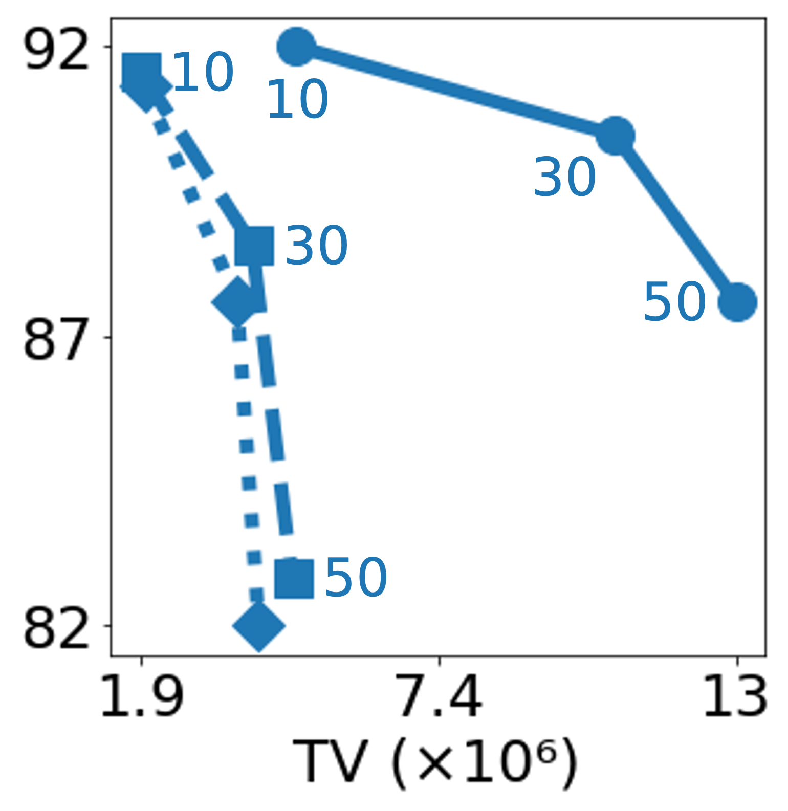
(a) Grad²

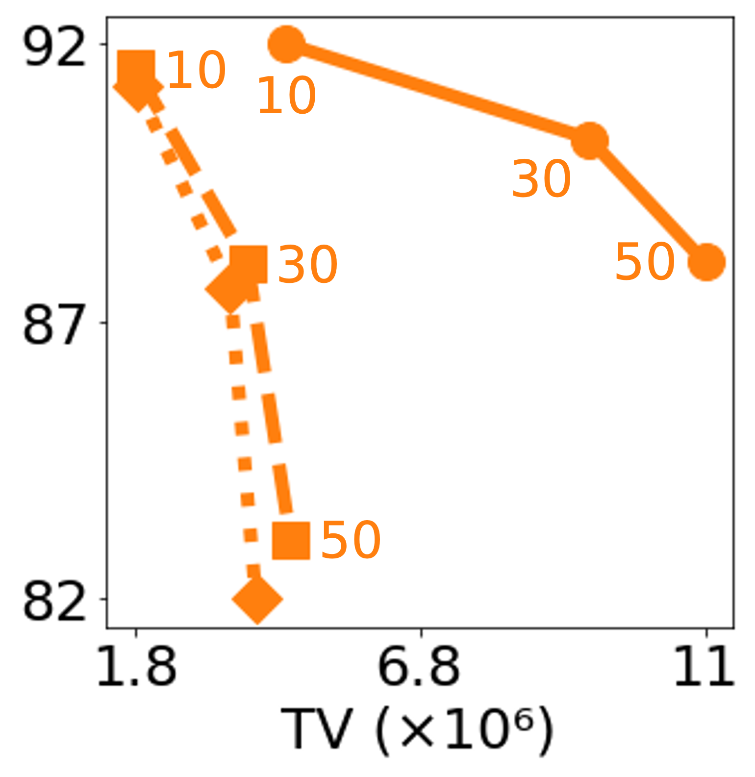
(b) GI²

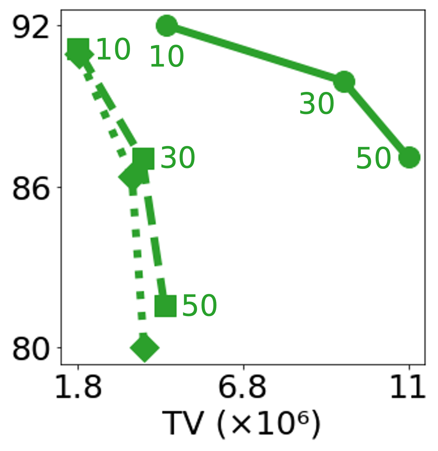
(c) IG²

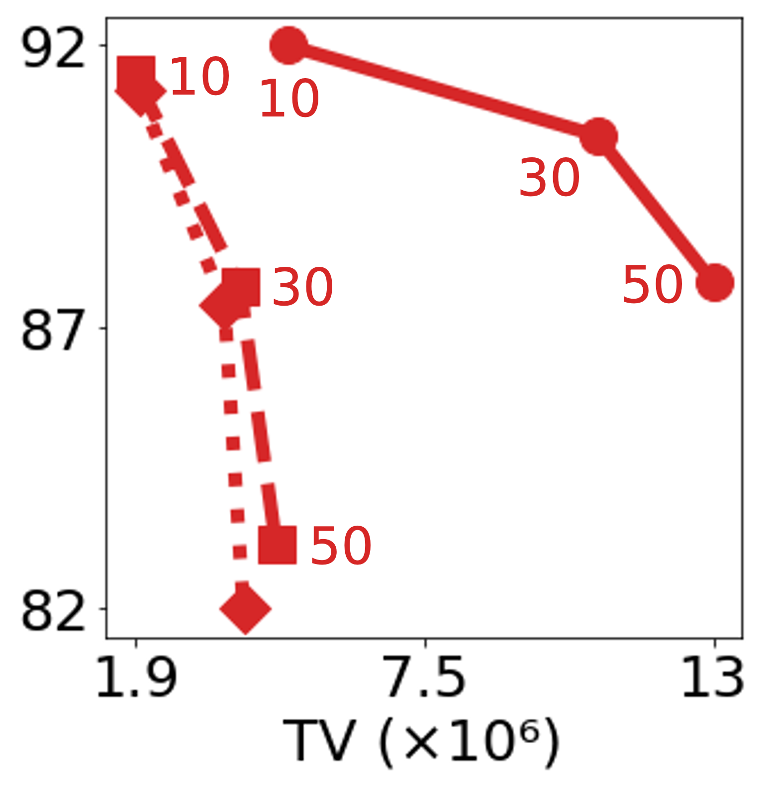
(d) SG²

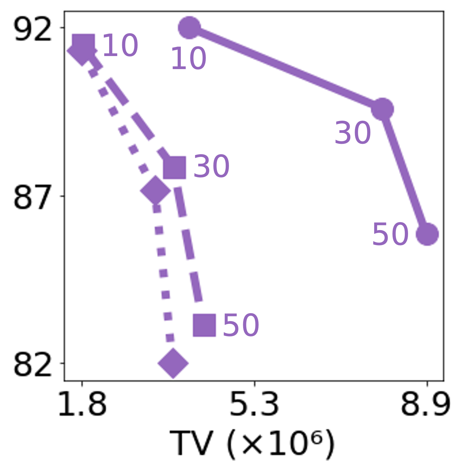
(e) SG-SQ

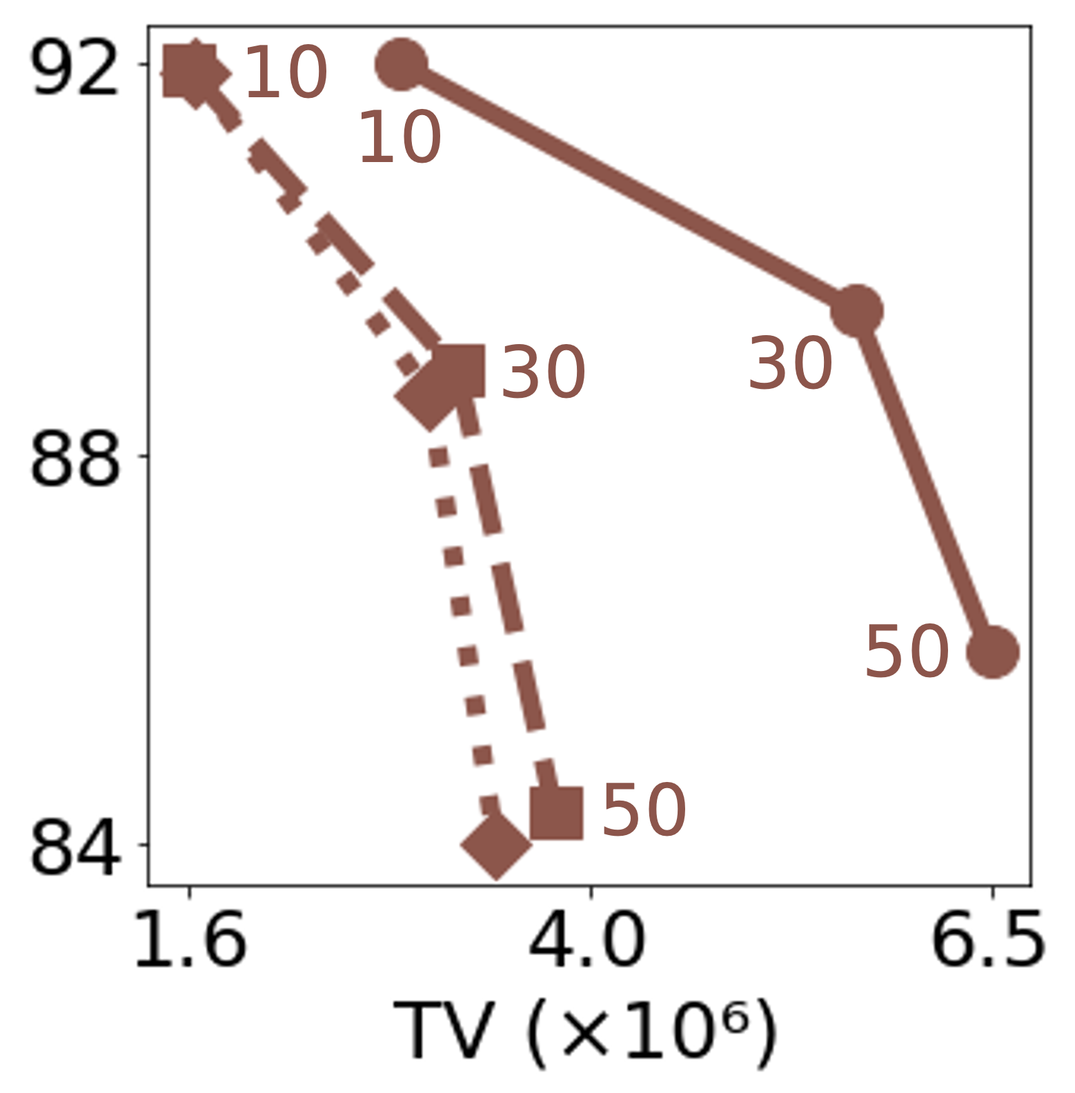
(f) VG

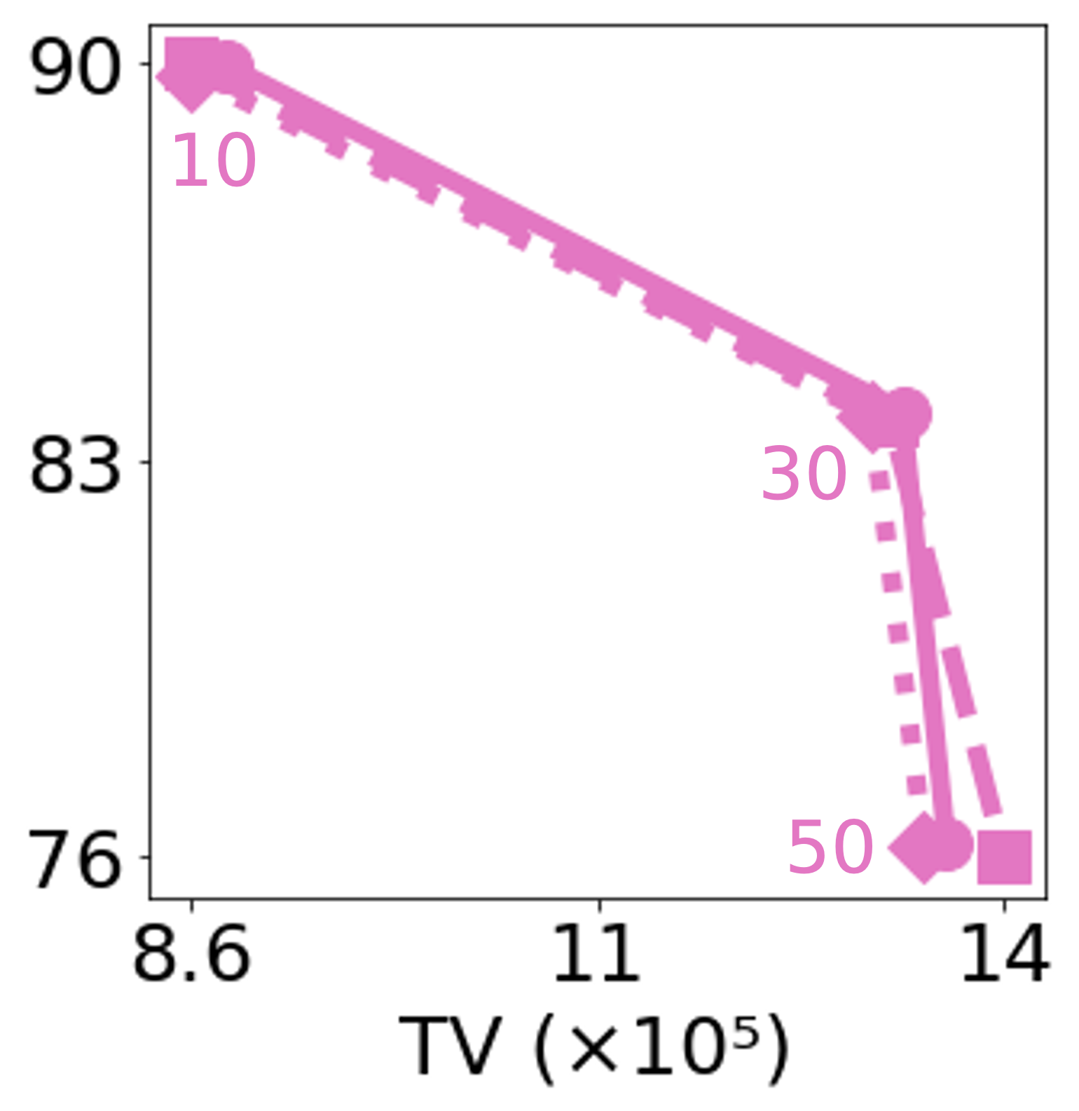
(g) GC²

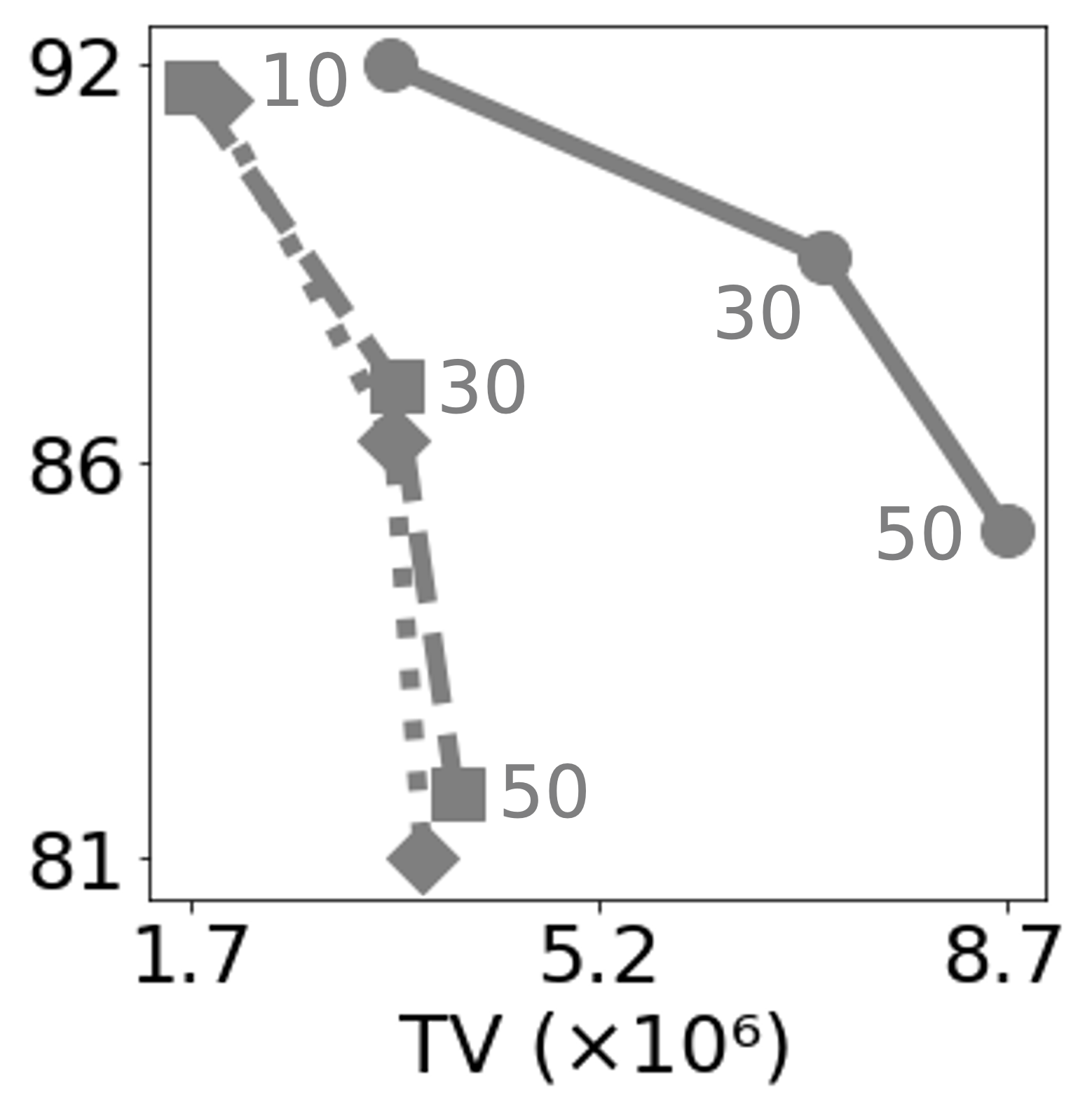
(h) Sobel²

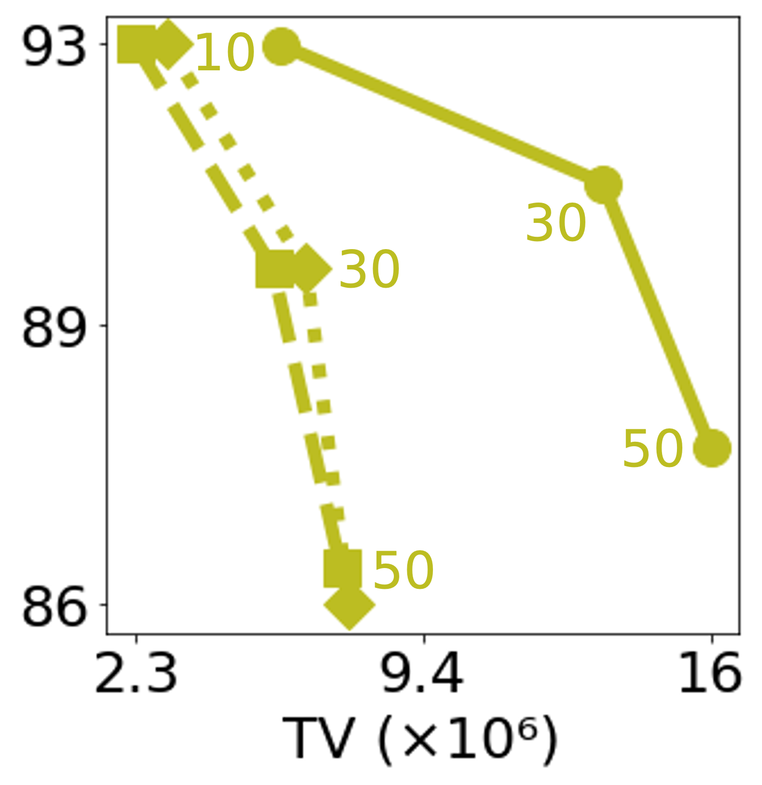
(i) Rand

Figure 8: Effects of Gaussian filtering and max-pooling on total variation of attribution masks and model accuracy on CIFAR-10.

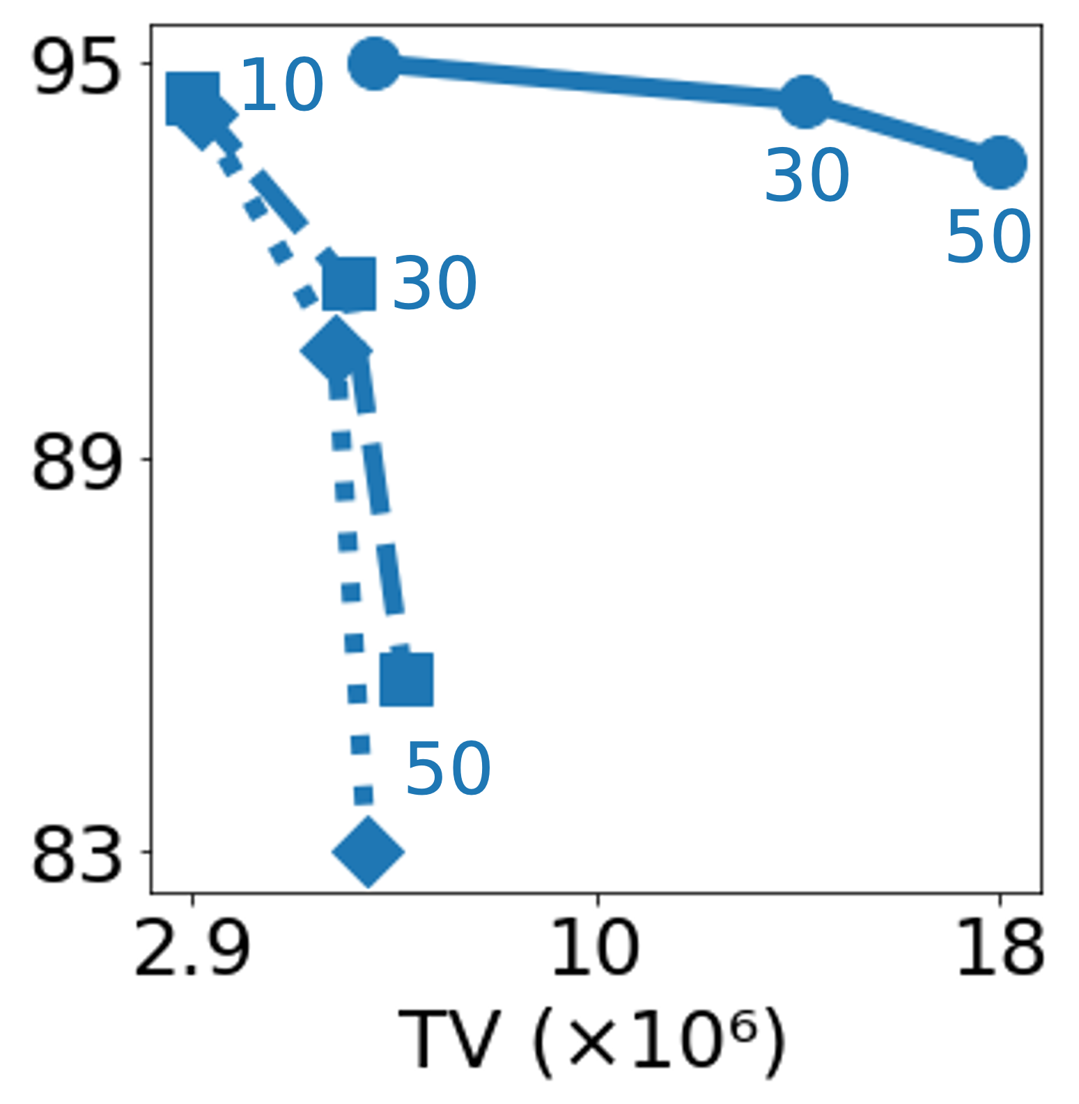
(a) Grad²

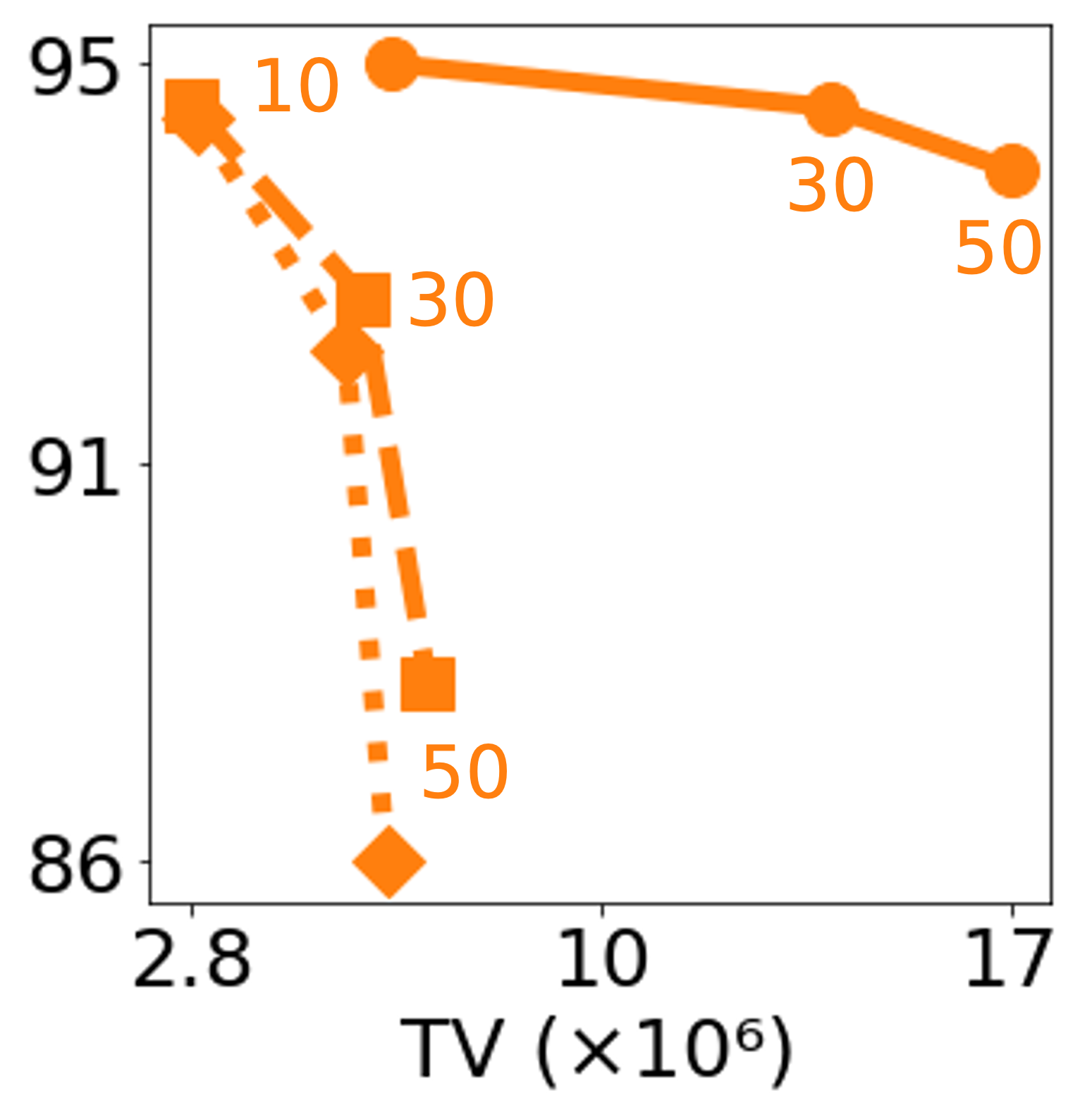
(b) GI²

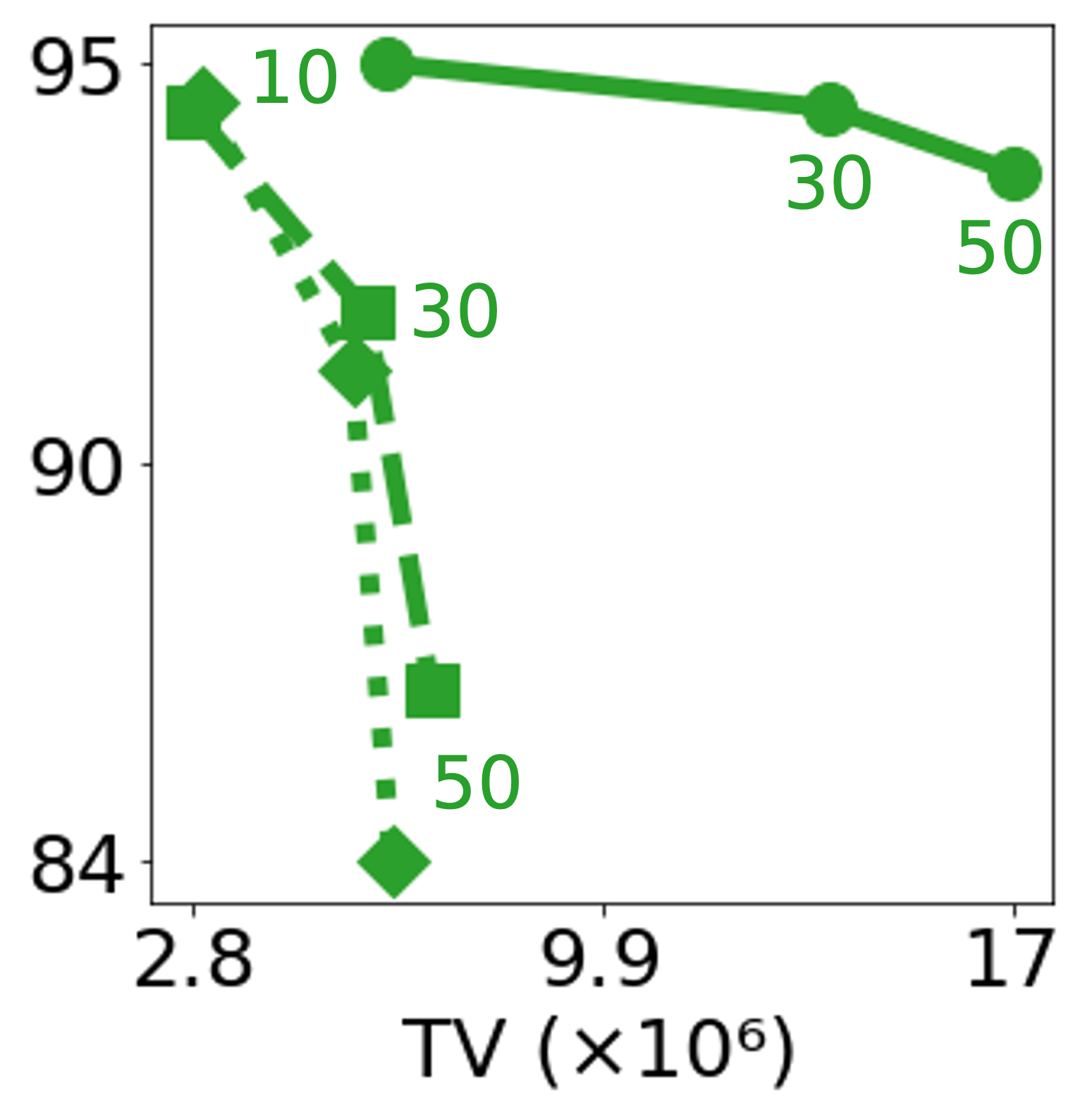
(c) IG²

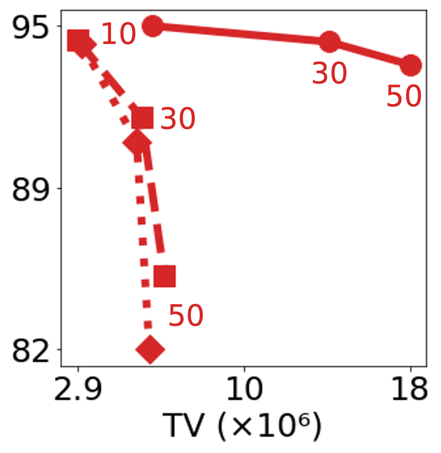
(d) SG²

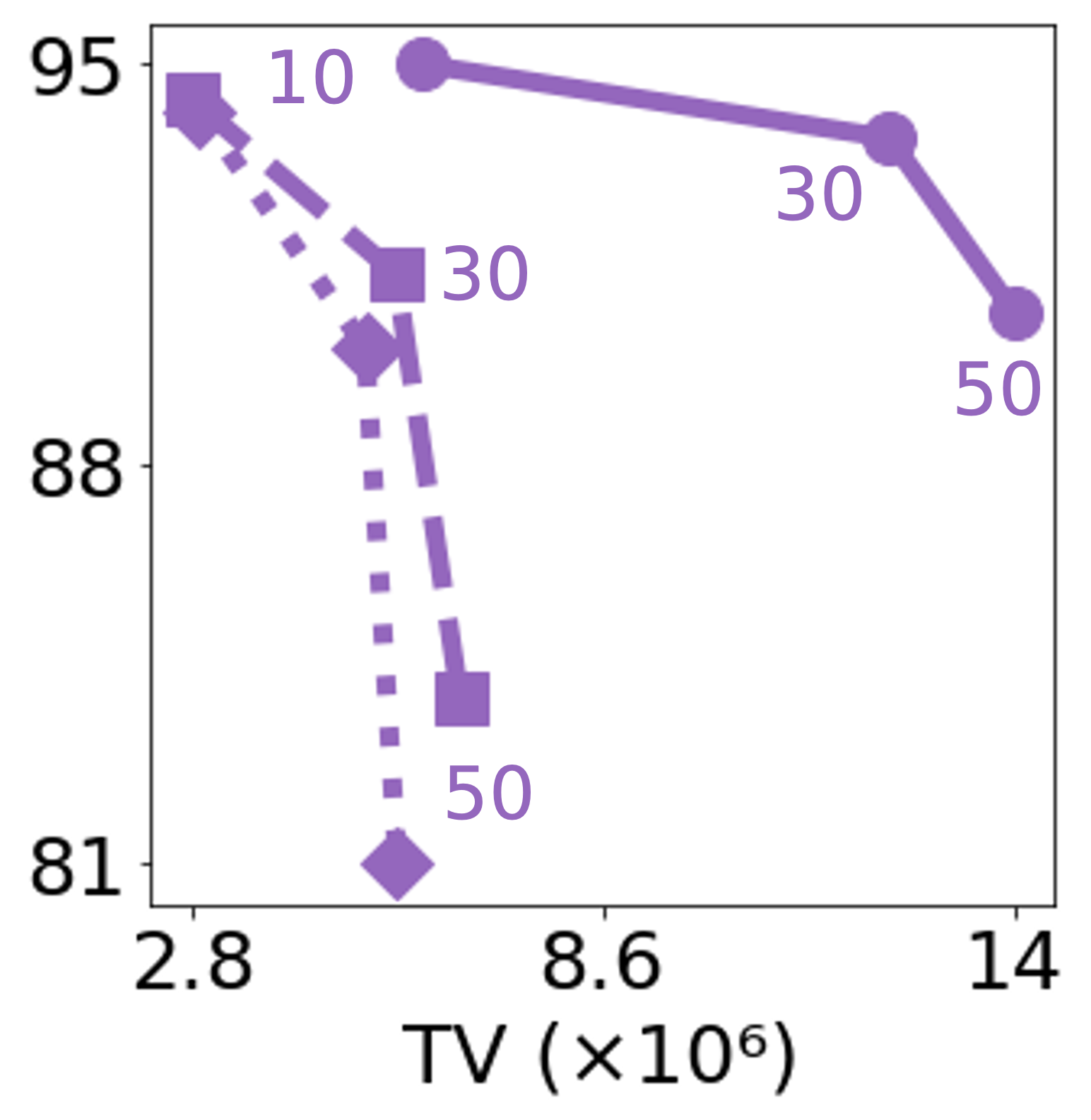
(e) SG-SQ

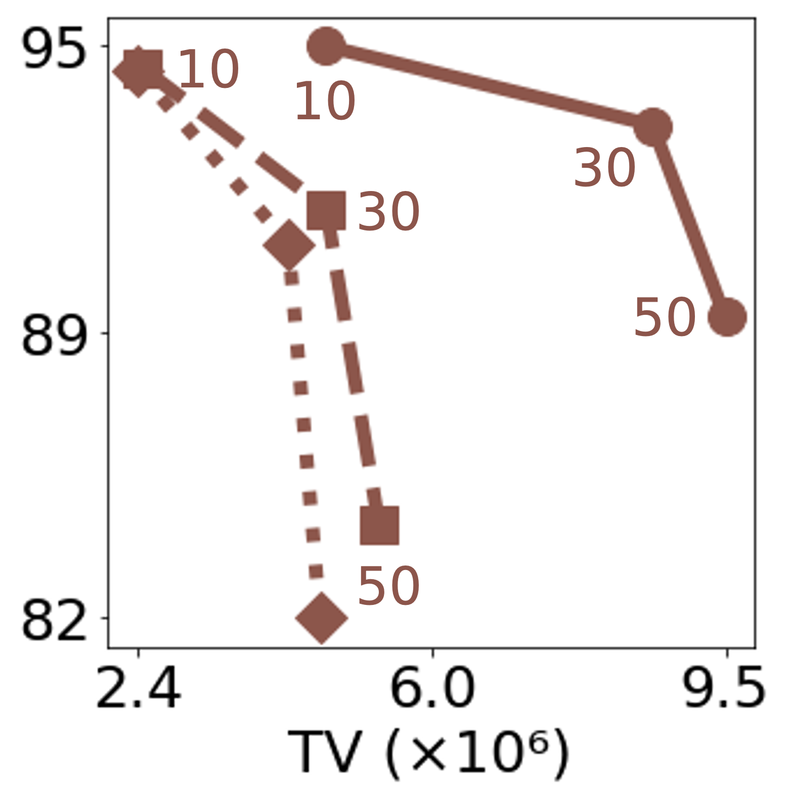
(f) VG

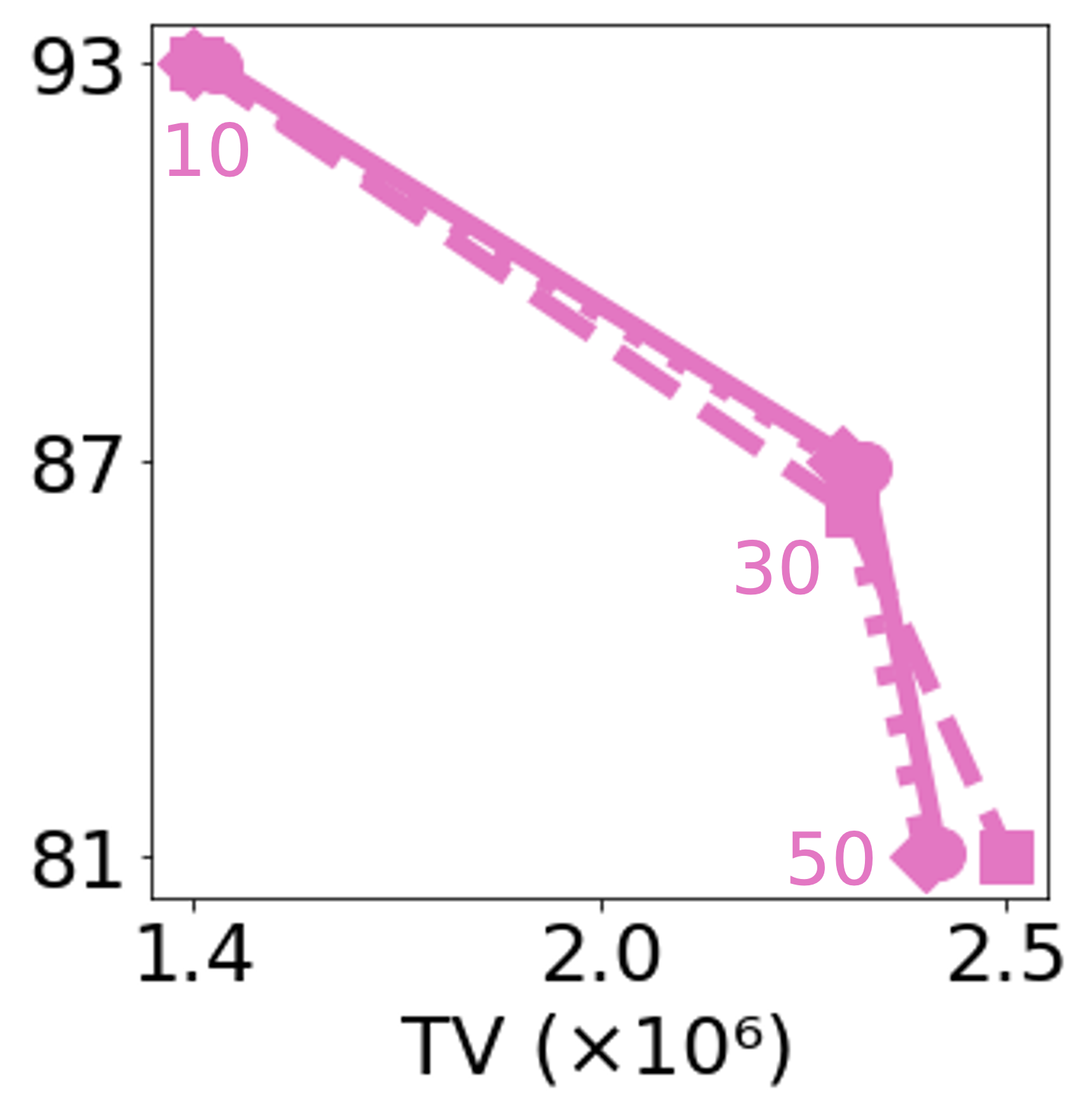
(g) GC²

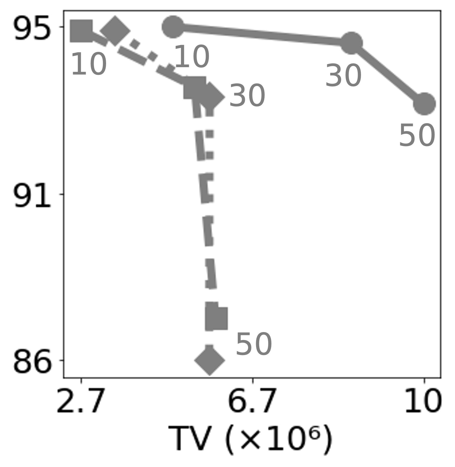
(h) Sobel²

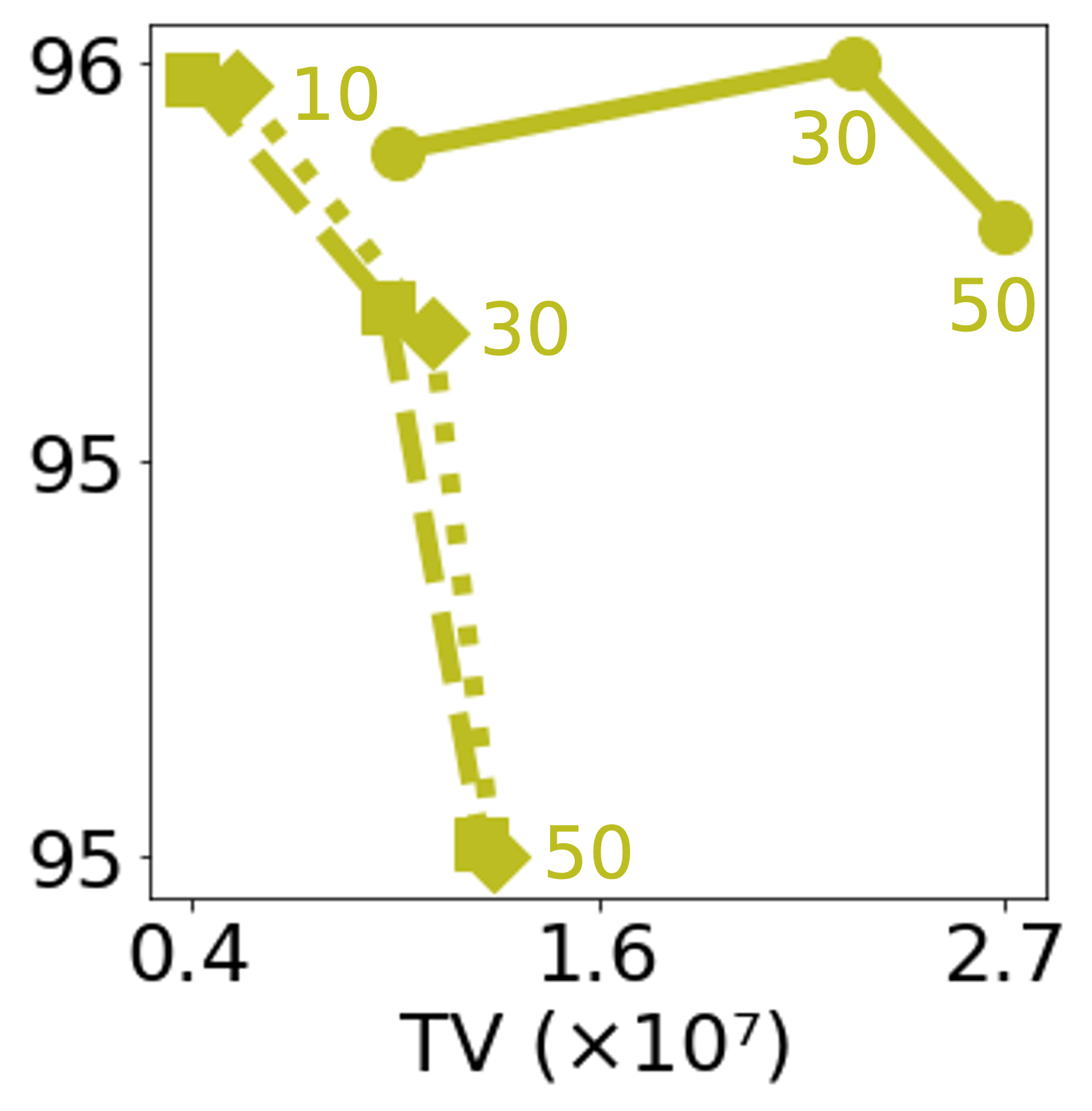
(i) Rand

Figure 9: Effects of Gaussian filtering and max-pooling on total variation of attribution masks and model accuracy on SVHN.

Going further, we aim to examine the relationship between the ROAR metric and the blurriness of attribution, as discussed in Section 3.2. To determine this relationship, we calculate the average total variation of attributions for the training set $A_{train}$ for each trial in the ROAR evaluation. The results, shown in Figure 7, demonstrate a strong negative correlation between the blurriness of attributions and the model’s performance in the ROAR protocol. Results of the experiment conducted on the CIFAR-10 and SVHN datasets can be found in Figures 8 and 9 of the supplementary material.

Our findings indicate that for most attribution methods and drop rates, max-pooling and Gaussian filtering reduce both the total variation and the model’s performance. However, this trend does not hold for the GC² method, as its unique approach - derived from gradients on intermediate feature maps rather than back-propagation on inputs - results in attribution maps with a smaller resolution, which are not impacted by degradation $k(\cdot)$. Similar patterns were observed in the CIFAR-10 and SVHN datasets (as shown in Figure 8 and Figure 9 in the supplementary material).

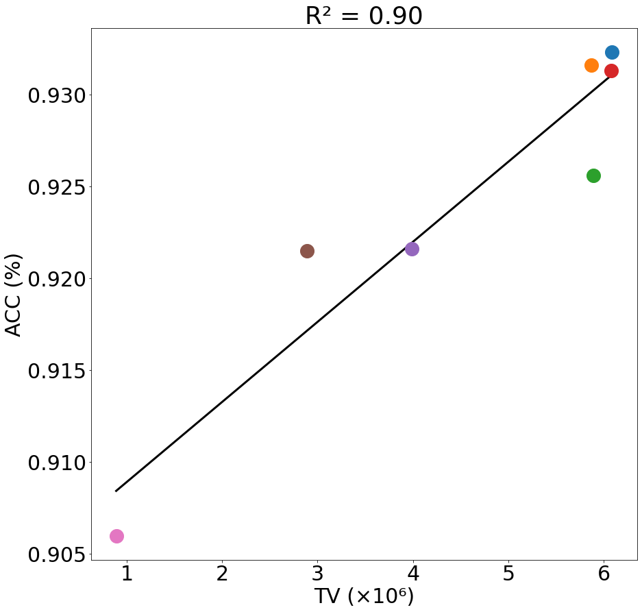
(a) $R^{2}=0.84$

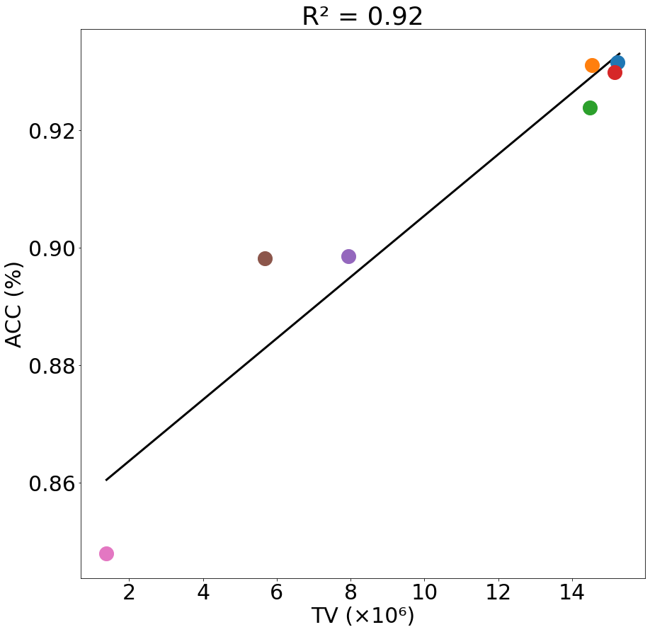
(b) $R^{2}=0.85$

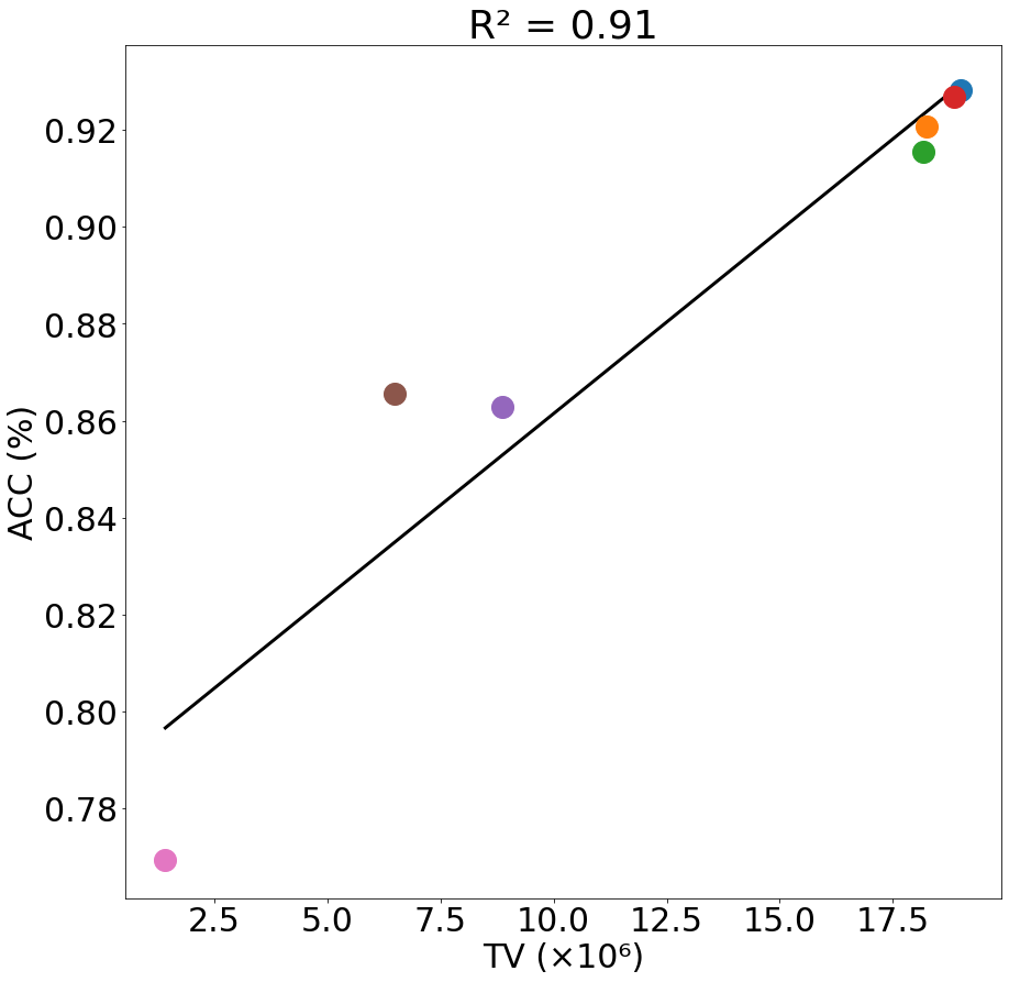
(c) $R^{2}=0.82$

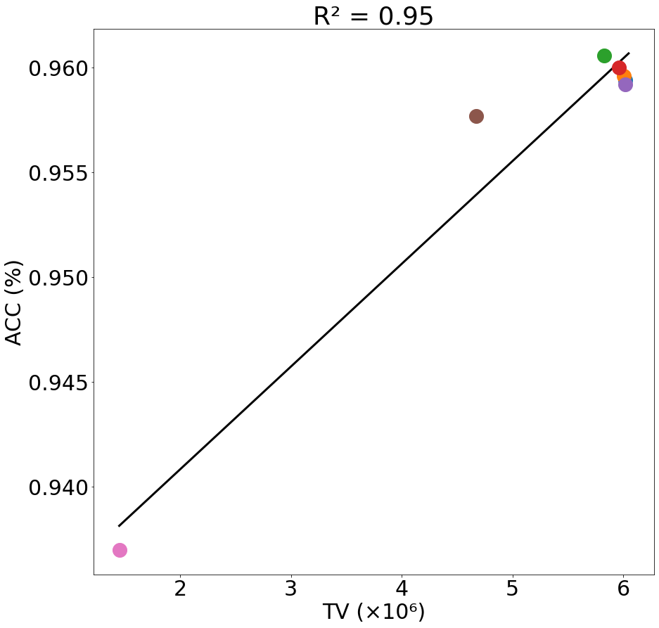
(d) $R^{2}=0.92$

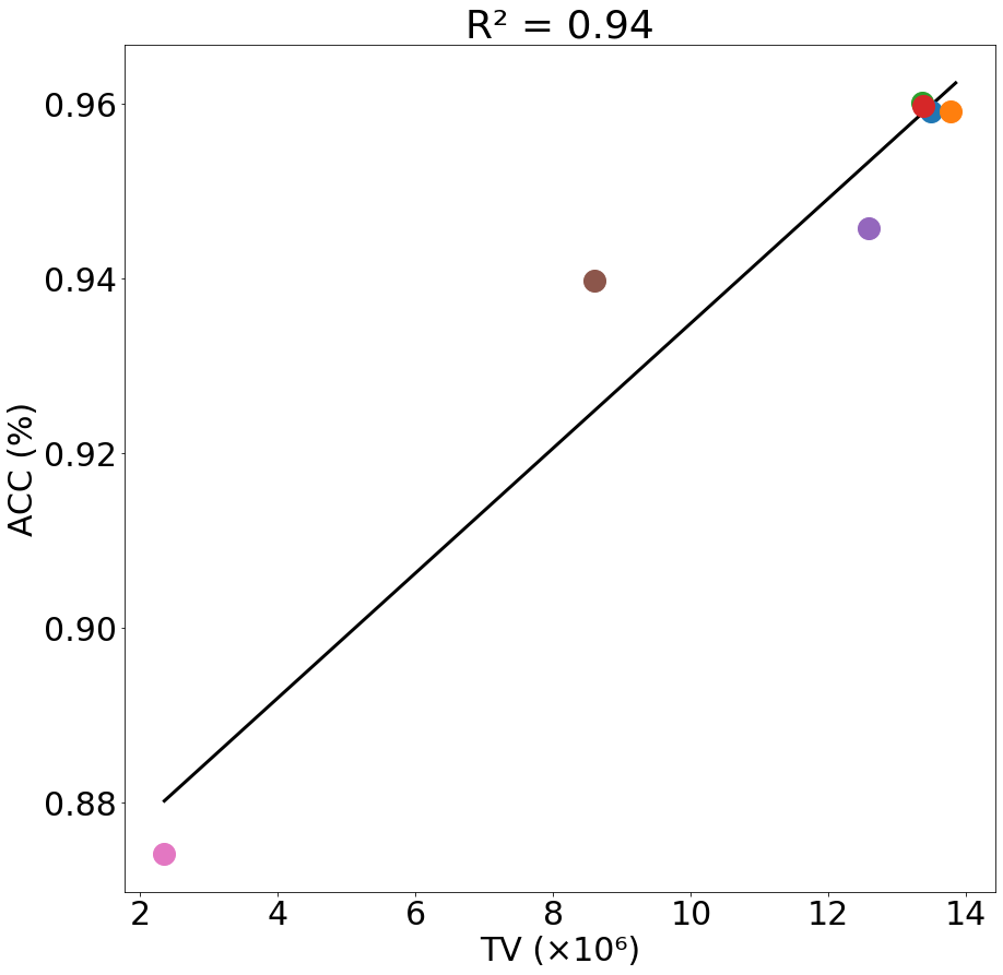
(e) $R^{2}=0.90$

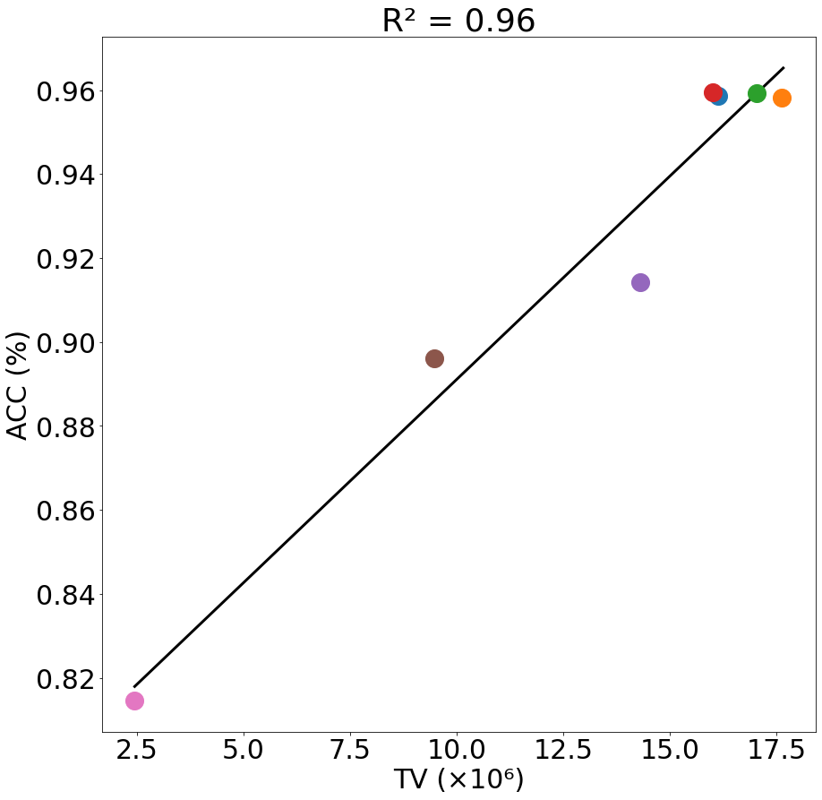
(f) $R^{2}=0.95$

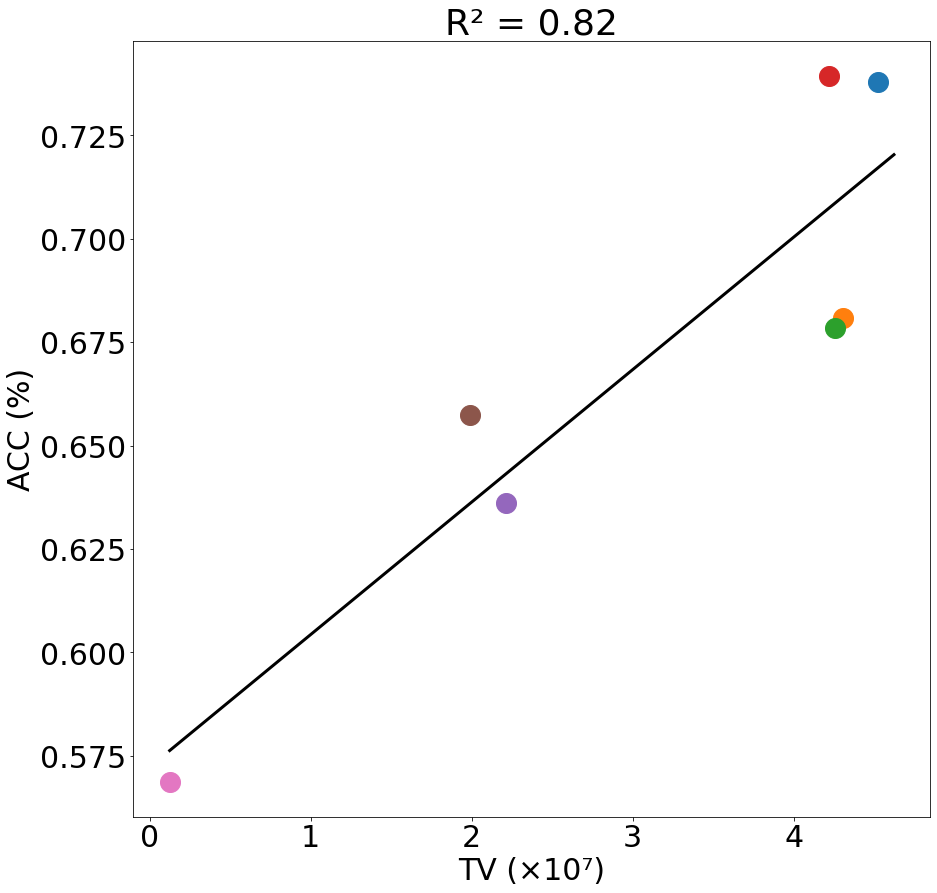
(g) $R^{2}=0.91$

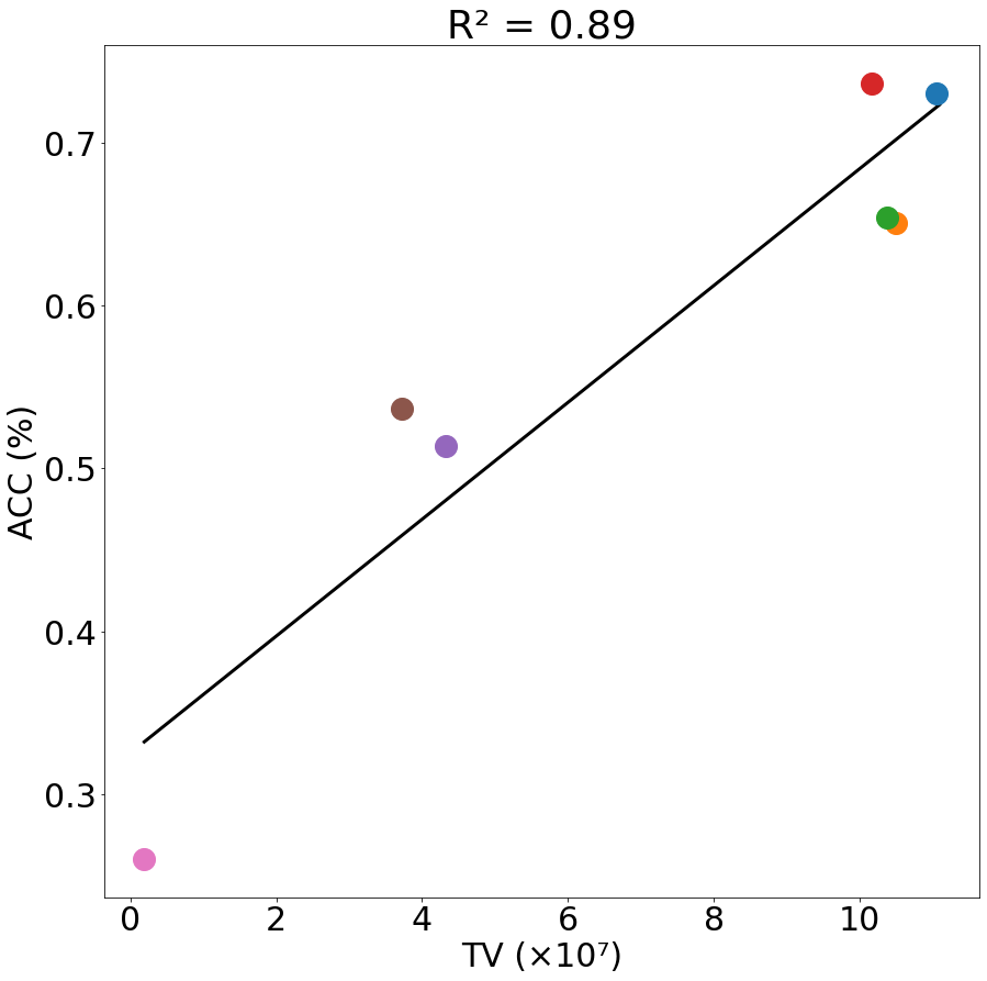
(h) $R^{2}=0.90$

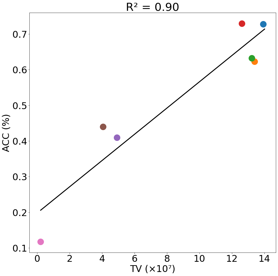
(i) $R^{2}=0.92$

Figure 10: Relationship between model accuracy and total variation of attribution masks (TV) in the aspect of non-squaring attribution method. The fitted line and coefficient of determination from simple linear regression are presented together. For all graphs, the y-axis represents the final test accuracy (%) in the ROAR evaluation protocol.

Next, we examine the relationship between the model’s performance and the total variation of attribution without post-processing. Figure 7 presents a scatter plot of all attribution methods’ results for each dataset and drop rate. It shows a strong linear correlation (ranging from $R^{2}=0.83$ to $R^{2}=0.96$) between the total variation of attribution and model accuracy, excluding results after post-processing. The corresponding results for the non-squared version of attribution methods can be found in Figure 10 of the supplementary material with the similar observation. We can thus conclude that there is a strong positive correlation between the blurriness of attribution and the ROAR benchmark, regardless of whether post-processing is applied or not.

(a) Grad²

(b) GI²

(c) IG²

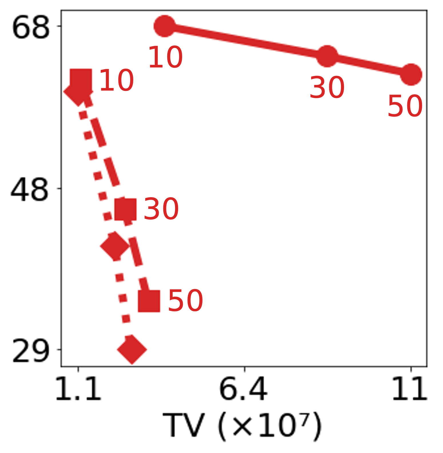
(d) SG²

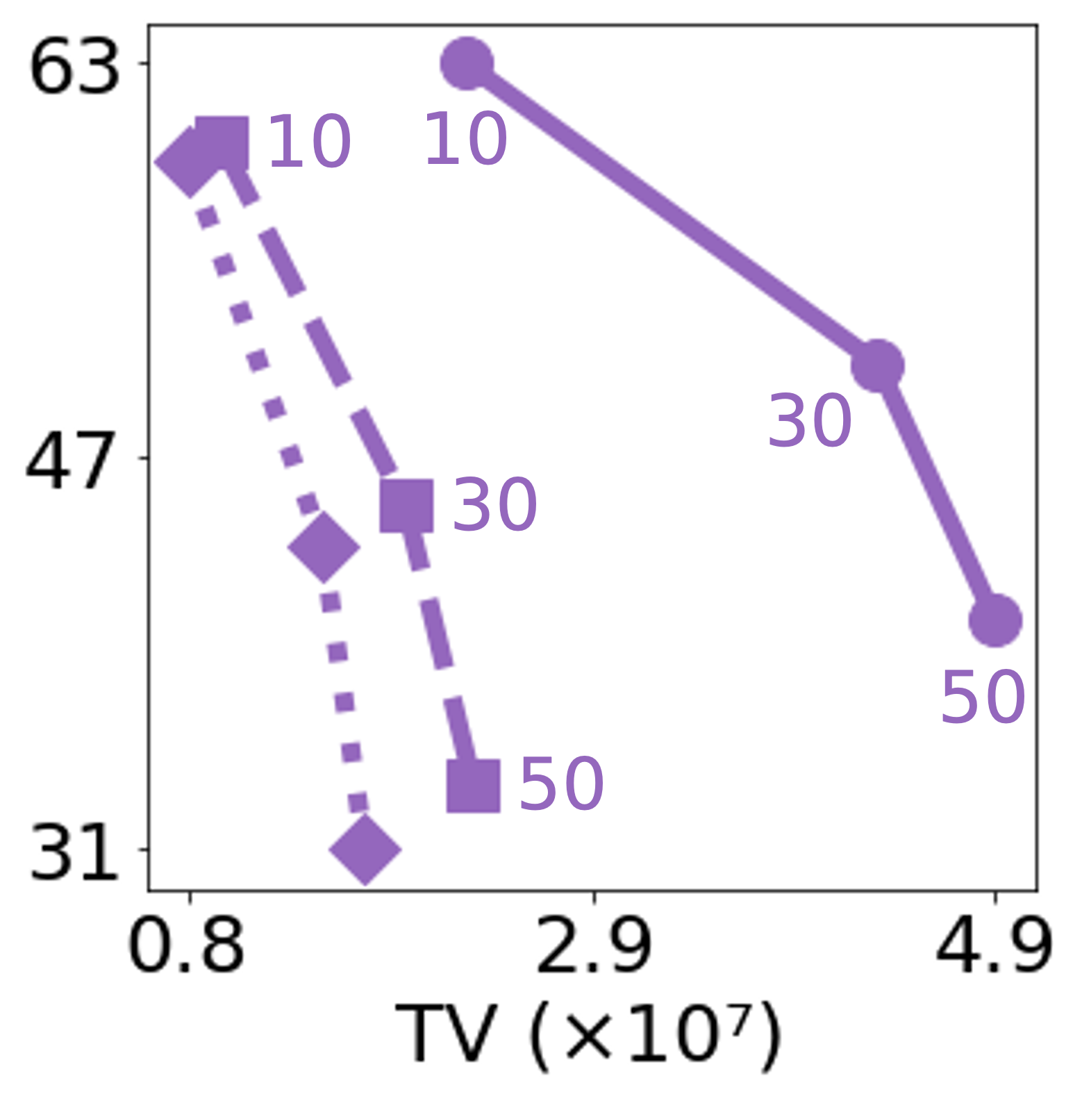
(e) SG-SQ

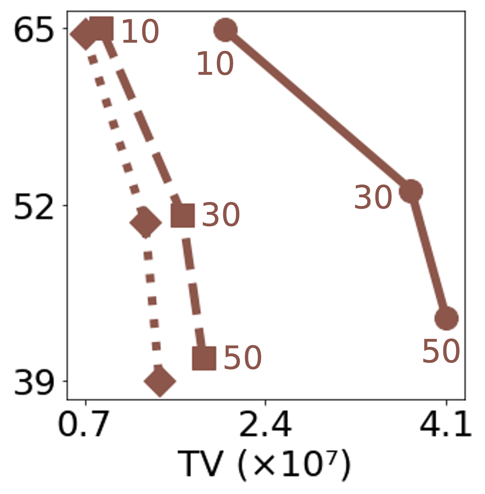
(f) VG

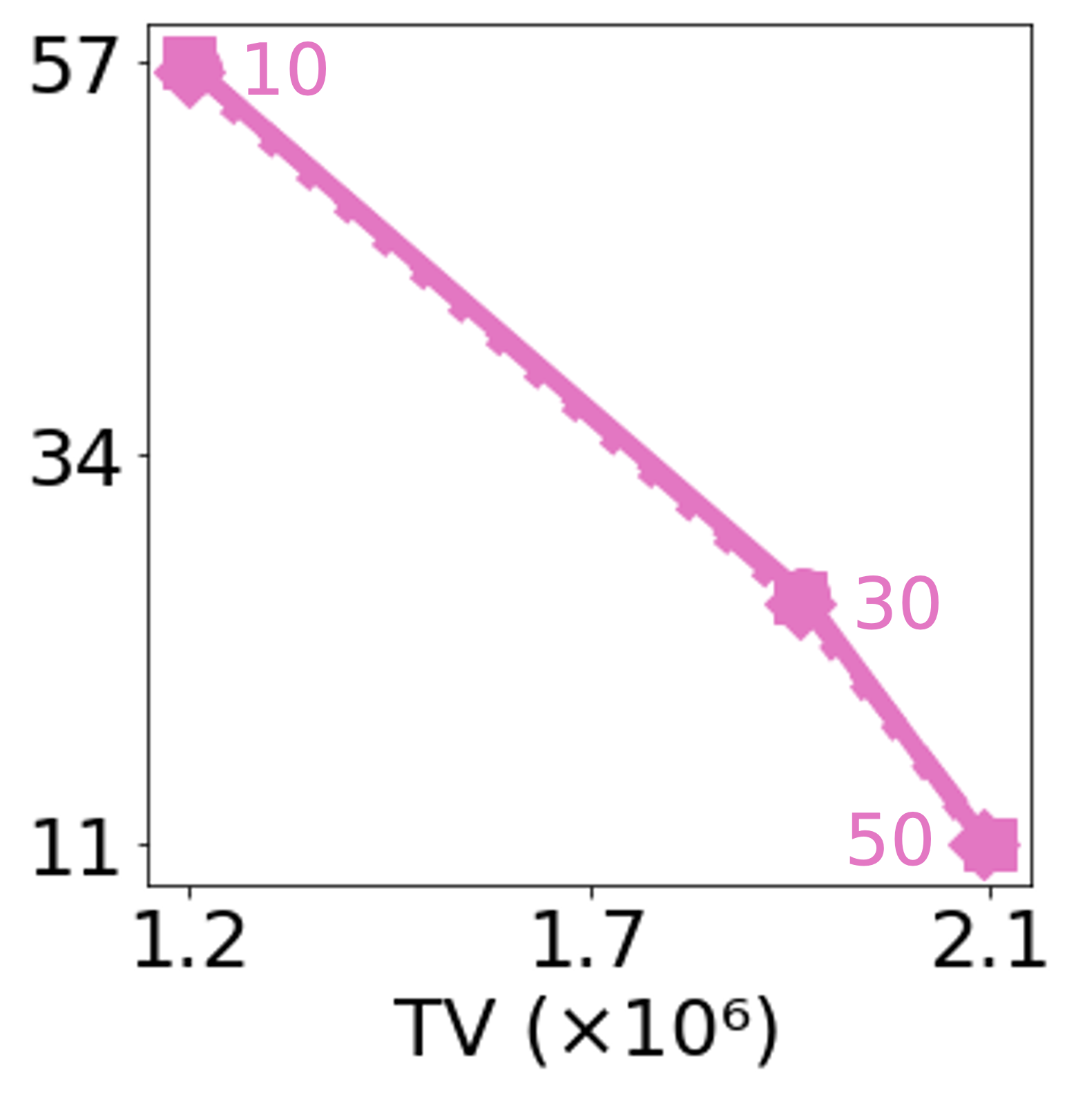
(g) GC²

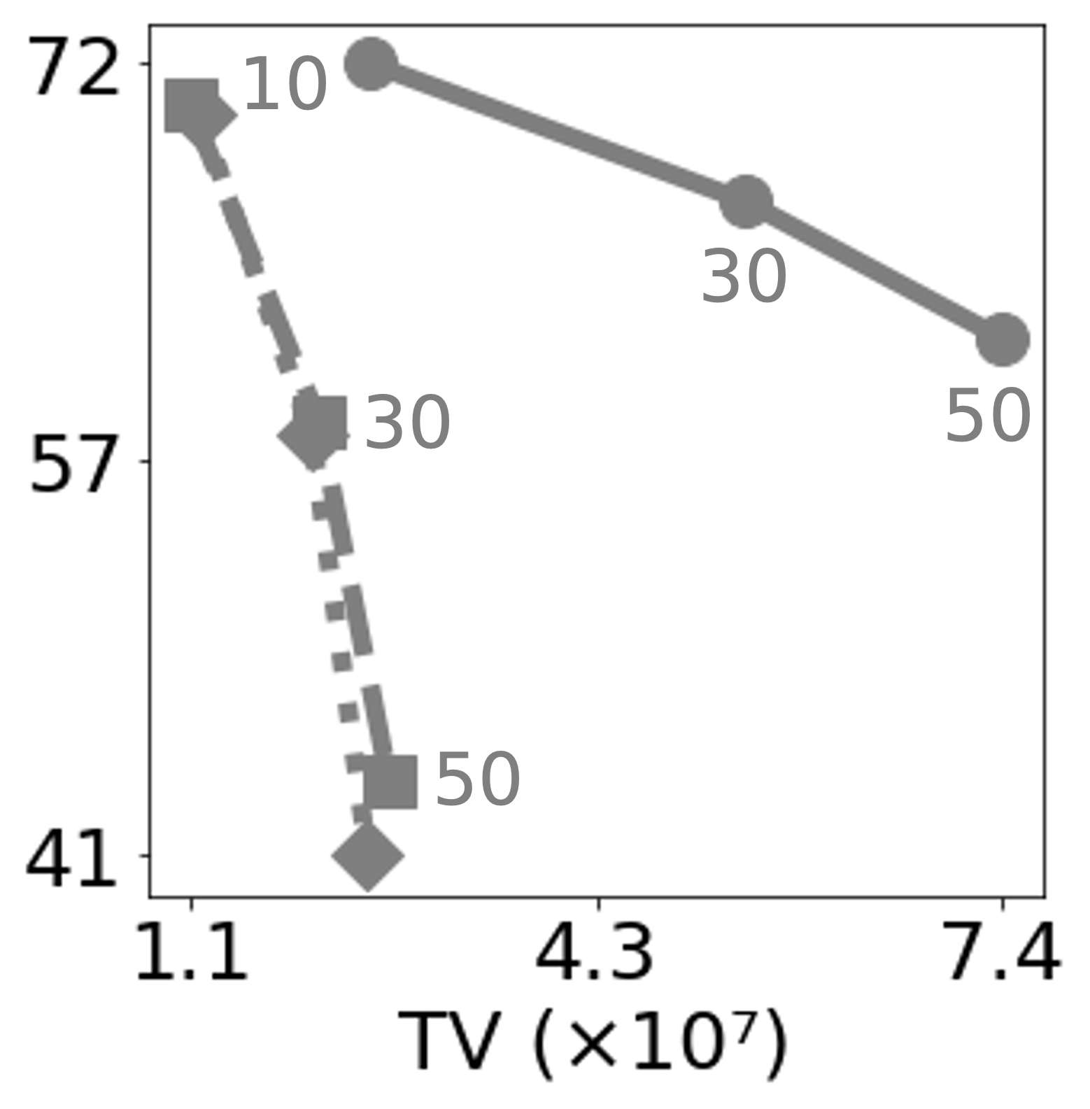
(h) Sobel²

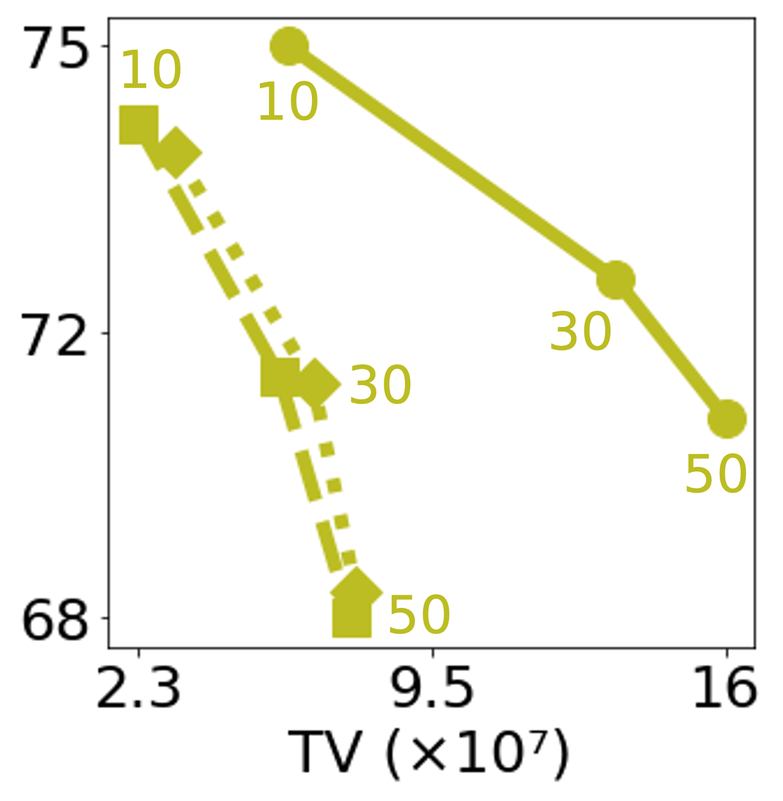
(i) Rand

Figure 6: Effects of Gaussian filtering and max-pooling on the total variation of attribution masks (TV) and model accuracy on the CUB-200 dataset. The number displayed above each point indicates the attribution drop rate. The y-axis in all graphs represents the final test accuracy (%) as measured by the ROAR evaluation protocol.

	10%	30%	50%
CIFAR-10
SVHN
CUB-200

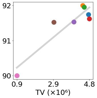
(a) $R^{2}=0.84$

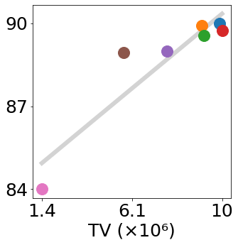
(b) $R^{2}=0.85$

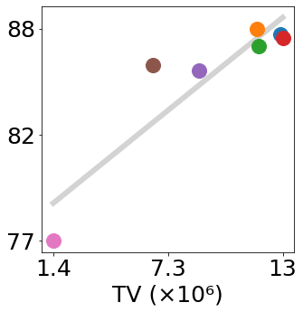
(c) $R^{2}=0.82$

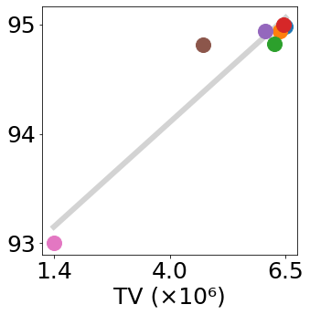
(d) $R^{2}=0.92$

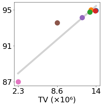
(e) $R^{2}=0.90$

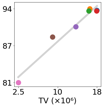
(f) $R^{2}=0.95$

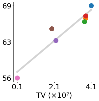
(g) $R^{2}=0.91$

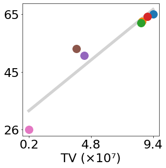
(h) $R^{2}=0.90$

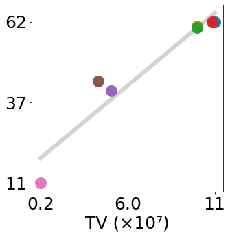
(i) $R^{2}=0.92$

Figure 7: The relationship between model accuracy and the total variation of attribution masks in terms of attribution method. The fitted line and coefficient of determination from simple linear regression are also included. The y-axis in all graphs represents the final test accuracy (%) as measured by the ROAR evaluation protocol.

5 Related Works

There has been an extensive body of research aimed at evaluating the quality of attribution methods, as noted in Nauta et al. (2022). As outlined by Doshi-Velez and Kim (2017), the evaluation of interpretability can be categorized into three distinct approaches based on the complexity of the task and the level of human involvement: functionally-grounded evaluation, human-grounded evaluation, and application-grounded evaluation. Further categorization of functionally-grounded evaluations into five subtypes was proposed by Zhou et al. (2021): clarity, broadness, simplicity, completeness, and soundness. On In this study, our focus is on the ROAR evaluation protocol Hooker et al. (2019), one of the widely-used, functionally-grounded, and soundness-oriented evaluation methodologies.

The ROAR evaluation protocol has been widely employed as a benchmarking method in various studies examining attribution methods. The ROAR protocol and its variants have been used to evaluate attribution methods across a range of tasks, including image domain tasks Chefer et al. (2021); Yang et al. (2020), natural language processing Ismail et al. (2021); Zhang et al. (2021), graph structure analysis Funke et al. (2022), and time-series analysis Liang et al. (2020); Ismail et al. (2020). The ROAR protocol has been established as the primary evaluation methodology in Meng et al. (2022)’s newly proposed standard benchmark on attribution methods. However, our research diverges from the recent trend and focuses on the intriguing and unintended behavior of the ROAR evaluation protocol.

Existing Discussions on the Limitations of ROAR

The limitations of the ROAR evaluation protocol have been discussed previously, as noted by Hooker et al. (2019). The authors pointed out that feature redundancy can result in an inability to distinguish between meaningless attributions and redundant input features when there is no performance degradation due to feature removal. However, no such phenomenon has been observed in real datasets. Our study aims to examine the legitimacy of the fundamental design intent of the ROAR protocol through a examination of the data generation process and real dataset experiments.

Recently, Rong et al. (2022) highlighted the issue of information leakage due to the mask shape. The study posits that the mask shape itself can contain class information, calling into question the validity of removal-based evaluation strategies like ROAR. To address these concerns, the authors perform an information-theoretic analysis and propose a novel evaluation framework called "RemOve-And-Debias (ROAD)". This framework reduces the impact of confounding factors in the ROAR evaluation metric, resulting in more consistent evaluation results. However, our findings address a different issue, namely the dependency of the data generation process, rather than the information leakage through the mask, which was the focus of Rong et al. (2022). Because the data generation process in ROAD is same to that of ROAR (as depicted in Figure 1), our discussion in Section 3.1 remains applicable to ROAD and our experimental results show the same tendency (See Section 4.2).

6 Discussion

Practical Takeaways

Our work does not aim to discourage the use of ROAR (or ROAD) in future research, but rather to emphasize the importance of exercising caution when employing and interpreting these methods. We present two main practical takeaways for the reader to consider.

• Superiority of sensitivity among attribution methods cannot be solely determined based on the ROAR benchmark results. Relying exclusively on these results could lead to misleading interpretations of the performance and sensitivity of attribution methods. A more appropriate approach to reporting performance using the ROAR benchmark is to include measurements of factors that can contribute to performance bias of the ROAR, as demonstrated in Fig. 7.

• Trend of the ROAR benchmark is partly influenced by the nature of the data, independent of whether the models and explainers are functioning correctly. It is important to note that such biases may manifest differently in other domains, although this study specifically addresses the bias of ROAR associated with image data. For instance, a similar relationship between data structure and feature redundancy has been reported in various domains, including time series Radovic et al. (2017) and graph structures Liu et al. (2022).

Extension to perturbation-based Evaluation Methods

The evaluation of the correctness of explanations assesses the quality of local feature attributions in predictive models, which are used to provide insight into a model’s decision-making processes Nauta et al. (2022). This evaluation is usually accomplished through perturbation-based methods, in which features are removed or altered from the input and the resulting changes in the model’s output are analyzed. The primary objective of this evaluation is to ensure that the explanations are readily understandable, as they should require a minimal set of features to alter the model’s predictions Samek et al. (2016); Yeh et al. (2019); Bhatt et al. (2020); Ismail et al. (2020).

While our work primarily focuses on the ROAR and ROAD methods, the findings and discussions are extensible to other perturbation-based evaluation methods that assess the correctness of attribution methods through changes in the predictive model’s output. This is because the core issue addressed in this study, which is the fundamental problem inherent in the data generation process during perturbation-based evaluations, is applicable to these methods as well. To the best of our knowledge, there are no exceptions to this principle in the existing perturbation-based evaluation methods. In future work, we plan to expand the scope of this discussion to encompass a broader range of perturbation-based evaluation methods beyond ROAR and ROAD.

Broader Impacts and Limitations

In this work, we have highlighted the shortcomings of the ROAR evaluation protocol and its variant ROAD, however, we have not proposed a method to rectify these issues. This limitation may lead to short-term confusion in the criteria for benchmarking existing attribution methods. We also acknowledge that our findings are primarily focused on image tasks, where the spatiality of features is strongly expressed. Despite these limitations, we emphasize that our intention is not to discourage the use of ROAR or ROAD in future research, but rather to encourage caution when employing and interpreting these methods. We aim to provide practical takeaways for readers, while also considering that our findings could potentially extend to other perturbation-based evaluation methods. We hope that by identifying these limitations, future research can explore methods to address the biases inherent in the data generation process during perturbation-based evaluations, leading to more reliable and consistent benchmarking criteria across various domains.

7 Conclusion

In conclusion, this paper challenges the indiscriminate use of the RemOve-And-Retrain (ROAR) metric and its variant as a means of evaluating the performance of feature importance estimates. Through our theoretical consideration and extensive experiments, we demonstrate that attributions with limited information about the explainer and model can outperform ROAR benchmarks, contrary to the intended design of the ROAR evaluation protocol. Our findings also reveal a bias towards attribution bluriness in the ROAR metric, and we caution against the uncritical reliance on ROAR metrics without taking these results into consideration. We believe that our findings will be valuable for researchers in the field of model explainability, as they highlight the need for further investigation and refinement of evaluation metrics for attribution techniques.

Contributions

Junhwa Song was responsible for conducting all the data collection and experimental procedures in this paper. Keumgang Cha made a significant contribution by reporting that blurry attribution is advantageous in the ROAR benchmark. Junghoon Seo played a key role in the overall drafting and design of the experiments, and also provided a comprehensive theoretical analysis.

Appendix A Details of Experiment Setting

All models were trained for 50 epochs with batch size $b=128$ except for $b=32$ on CUB-200 Welinder et al. [2010] on a single GTX1080Ti GPU. Each model was trained with SGD optimizer with momentum $\beta=0.9$ and weight decay $\lambda=1\times 10^{-4}$ except for $\lambda=5\times 10^{-4}$ on CIFAR-10. To avoid convergence on bad local minima, cosine annealing scheduling Loshchilov and Hutter [2017] was used, starting from the initial learning rate $\alpha=0.1$ for CIFAR-10 and SHVN. For CUB-200, $\alpha=0.01$ was used. The learning rate was annealed to zero over 50 epochs. Especially in the case of CUB-200, we use ImageNet Deng et al. [2009] pre-trained model for fast convergence. In our ROAD Rong et al. [2022] experiments, we utilized MMClassification framework Contributors [2020] to facilitate the implementation. Our training strategies followed MMClassification’s ones for ResNet18 on CIFAR-10 and ResNet50 on CUB-200. In the case of SVHN, we adopted the same strategy as CIFAR-10.

Base estimators were implemented by PyTorch AutoGrad module. Similar to Hooker et al. [2019], in Integrated Gradients, interval $k$ is set to 25, and the reference image is set to zeros. Also, for the ensemble methodologies, the sample size is set to $n=15$. Among all estimators, only Sobel edge detector is implemented by SciPy library Virtanen et al. [2020]. Finally, we post-process attribution map using Maximum filter with kernel size $=3$ and Gaussian filter function with standard deviation for Gaussian kernel $\sigma=1$ in SciPy library.

Appendix B Additional Tables and Plots

	10%	30%	50%
CIFAR-10
SVHN
CUB-200

References

- Adebayo et al. [2018a] Julius Adebayo, Justin Gilmer, Ian Goodfellow, and Been Kim. Local explanation methods for deep neural networks lack sensitivity to parameter values. In ICLR Workshop, 2018a.
- Adebayo et al. [2018b] Julius Adebayo, Justin Gilmer, Michael Muelly, Ian Goodfellow, Moritz Hardt, and Been Kim. Sanity checks for saliency maps. NeurIPS, 2018b.
- Adebayo et al. [2020] Julius Adebayo, Michael Muelly, Ilaria Liccardi, and Been Kim. Debugging tests for model explanations. In NeurIPS, 2020. URL https://proceedings.neurips.cc/paper/2020/hash/075b051ec3d22dac7b33f788da631fd4-Abstract.html.
- Ancona et al. [2018] Marco Ancona, Enea Ceolini, Cengiz Öztireli, and Markus Gross. Towards better understanding of gradient-based attribution methods for deep neural networks. In ICLR, 2018. URL https://openreview.net/forum?id=Sy21R9JAW.
- Bach et al. [2015] Sebastian Bach, Alexander Binder, Grégoire Montavon, Frederick Klauschen, Klaus-Robert Müller, and Wojciech Samek. On pixel-wise explanations for non-linear classifier decisions by layer-wise relevance propagation. PloS one, 10(7):e0130140, 2015.
- Baehrens et al. [2010] David Baehrens, Timon Schroeter, Stefan Harmeling, Motoaki Kawanabe, Katja Hansen, and Klaus-Robert Müller. How to explain individual classification decisions. JMLR, 11(61):1803–1831, 2010. URL http://jmlr.org/papers/v11/baehrens10a.html.
- Bhatt et al. [2020] Umang Bhatt, Adrian Weller, and José MF Moura. Evaluating and aggregating feature-based model explanations. In IJCAI, 2020.
- Chefer et al. [2021] Hila Chefer, Shir Gur, and Lior Wolf. Transformer interpretability beyond attention visualization. In CVPR, pages 782–791, 2021.
- Contributors [2020] MMClassification Contributors. Openmmlab’s image classification toolbox and benchmark. https://github.com/open-mmlab/mmclassification, 2020.
- Dabkowski and Gal [2017] Piotr Dabkowski and Yarin Gal. Real time image saliency for black box classifiers. In NeurIPS, 2017.
- Deng et al. [2009] Jia Deng, Wei Dong, Richard Socher, Li-Jia Li, Kai Li, and Li Fei-Fei. Imagenet: A large-scale hierarchical image database. In CVPR, 2009.
- DeYoung et al. [2020] Jay DeYoung, Sarthak Jain, Nazneen Fatema Rajani, Eric Lehman, Caiming Xiong, Richard Socher, and Byron C. Wallace. ERASER: A benchmark to evaluate rationalized NLP models. In ACL, 2020.
- Doshi-Velez and Kim [2017] Finale Doshi-Velez and Been Kim. Towards a rigorous science of interpretable machine learning. arXiv preprint arXiv:1702.08608, 2017.
- Fong and Vedaldi [2017] Ruth C Fong and Andrea Vedaldi. Interpretable explanations of black boxes by meaningful perturbation. In ICCV, pages 3429–3437, 2017.
- Funke et al. [2022] Thorben Funke, Megha Khosla, Mandeep Rathee, and Avishek Anand. Zorro: Valid, sparse, and stable explanations in graph neural networks. IEEE Transactions on Knowledge and Data Engineering, 2022.
- Hartley et al. [2021] Thomas Hartley, Kirill Sidorov, Christopher Willis, and David Marshall. Swag: Superpixels weighted by average gradients for explanations of cnns. In WACV, pages 423–432, 2021.
- He et al. [2016] Kaiming He, Xiangyu Zhang, Shaoqing Ren, and Jian Sun. Deep residual learning for image recognition. In CVPR, pages 770–778, 2016.
- Hellman and Raviv [1970] Martin Hellman and Josef Raviv. Probability of error, equivocation, and the chernoff bound. IEEE Transactions on Information Theory, 16(4):368–372, 1970.
- Hooker et al. [2019] Sara Hooker, Dumitru Erhan, Pieter-Jan Kindermans, and Been Kim. A benchmark for interpretability methods in deep neural networks. In NeurIPS, pages 9737–9748, 2019.
- Ismail et al. [2020] Aya Abdelsalam Ismail, Mohamed Gunady, Héctor Corrada Bravo, and Soheil Feizi. Benchmarking deep learning interpretability in time series predictions. In NeurIPS, 2020.
- Ismail et al. [2021] Aya Abdelsalam Ismail, Hector Corrada Bravo, and Soheil Feizi. Improving deep learning interpretability by saliency guided training. NeurIPS, 34, 2021.
- Khakzar et al. [2021] Ashkan Khakzar, Soroosh Baselizadeh, Saurabh Khanduja, Christian Rupprecht, Seong Tae Kim, and Nassir Navab. Neural response interpretation through the lens of critical pathways. In CVPR, pages 13528–13538, 2021.
- Kim et al. [2019a] Beomsu Kim, Junghoon Seo, Seunghyeon Jeon, Jamyoung Koo, Jeongyeol Choe, and Taegyun Jeon. Why are saliency maps noisy? cause of and solution to noisy saliency maps. In ICCV Workshop, pages 4149–4157. IEEE, 2019a.
- Kim et al. [2019b] Beomsu Kim, Junghoon Seo, and Taegyun Jeon. Bridging adversarial robustness and gradient interpretability. ICLR Workshop, 2019b.
- Krizhevsky et al. [2009] Alex Krizhevsky et al. Learning multiple layers of features from tiny images. 2009.
- Liang et al. [2020] Jian Liang, Bing Bai, Yuren Cao, Kun Bai, and Fei Wang. Adversarial infidelity learning for model interpretation. In KDD, page 286–296, 2020. ISBN 9781450379984. URL https://doi.org/10.1145/3394486.3403071.
- Liu et al. [2022] Xin Liu, Xunbin Xiong, Mingyu Yan, Runzhen Xue, Shirui Pan, Xiaochun Ye, and Dongrui Fan. Rethinking efficiency and redundancy in training large-scale graphs. arXiv preprint arXiv:2209.00800, 2022.
- Loshchilov and Hutter [2017] Ilya Loshchilov and Frank Hutter. Sgdr: Stochastic gradient descent with warm restarts. In ICLR, 2017.
- Lundberg and Lee [2017] Scott M Lundberg and Su-In Lee. A unified approach to interpreting model predictions. In I. Guyon, U. V. Luxburg, S. Bengio, H. Wallach, R. Fergus, S. Vishwanathan, and R. Garnett, editors, NeurIPS, volume 30. Curran Associates, Inc., 2017. URL https://proceedings.neurips.cc/paper/2017/file/8a20a8621978632d76c43dfd28b67767-Paper.pdf.
- Meng et al. [2022] Chuizheng Meng, Loc Trinh, Nan Xu, James Enouen, and Yan Liu. Interpretability and fairness evaluation of deep learning models on mimic-iv dataset. Scientific Reports, 12(1):1–28, 2022.
- Nauta et al. [2022] Meike Nauta, Jan Trienes, Shreyasi Pathak, Elisa Nguyen, Michelle Peters, Yasmin Schmitt, Jörg Schlötterer, Maurice van Keulen, and Christin Seifert. From anecdotal evidence to quantitative evaluation methods: A systematic review on evaluating explainable ai. arXiv preprint arXiv:2201.08164, 2022.
- Netzer et al. [2011] Yuval Netzer, Tao Wang, Adam Coates, Alessandro Bissacco, Bo Wu, and Andrew Y Ng. Reading digits in natural images with unsupervised feature learning. 2011.
- O’Shaughnessy et al. [2020] Matthew O’Shaughnessy, Gregory Canal, Marissa Connor, Mark Davenport, and Christopher Rozell. Generative causal explanations of black-box classifiers. NeurIPS, 2020.
- Radovic et al. [2017] Milos Radovic, Mohamed Ghalwash, Nenad Filipovic, and Zoran Obradovic. Minimum redundancy maximum relevance feature selection approach for temporal gene expression data. BMC bioinformatics, 18(1):1–14, 2017.
- Rong et al. [2022] Yao Rong, Tobias Leemann, Vadim Borisov, Gjergji Kasneci, and Enkelejda Kasneci. A consistent and efficient evaluation strategy for attribution methods. In ICML, pages 18770–18795. PMLR, 2022.
- Rudin et al. [1992] Leonid I Rudin, Stanley Osher, and Emad Fatemi. Nonlinear total variation based noise removal algorithms. Physica D: nonlinear phenomena, 60(1-4):259–268, 1992.
- Samek et al. [2016] Wojciech Samek, Alexander Binder, Grégoire Montavon, Sebastian Lapuschkin, and Klaus-Robert Müller. Evaluating the visualization of what a deep neural network has learned. TNNLS, 2016.
- Samek et al. [2021] Wojciech Samek, Grégoire Montavon, Sebastian Lapuschkin, Christopher J Anders, and Klaus-Robert Müller. Explaining deep neural networks and beyond: A review of methods and applications. Proceedings of the IEEE, 2021.
- Schramowski et al. [2020] Patrick Schramowski, Wolfgang Stammer, Stefano Teso, Anna Brugger, Franziska Herbert, Xiaoting Shao, Hans-Georg Luigs, Anne-Katrin Mahlein, and Kristian Kersting. Making deep neural networks right for the right scientific reasons by interacting with their explanations. Nature Machine Intelligence, 2020.
- Selvaraju et al. [2017] Ramprasaath R Selvaraju, Michael Cogswell, Abhishek Das, Ramakrishna Vedantam, Devi Parikh, and Dhruv Batra. Grad-cam: Visual explanations from deep networks via gradient-based localization. In CVPR, pages 618–626, 2017.
- Shrikumar et al. [2017] Avanti Shrikumar, Peyton Greenside, and Anshul Kundaje. Learning important features through propagating activation differences. In ICML, 2017.
- Simonyan et al. [2014] Karen Simonyan, Andrea Vedaldi, and Andrew Zisserman. Deep inside convolutional networks: Visualising image classification models and saliency maps. In ICLR Workshop, 2014.
- Smilkov et al. [2017] Daniel Smilkov, Nikhil Thorat, Been Kim, Fernanda Viégas, and Martin Wattenberg. Smoothgrad: removing noise by adding noise. ICML Workshop, 2017.
- Sundararajan et al. [2017] Mukund Sundararajan, Ankur Taly, and Qiqi Yan. Axiomatic attribution for deep networks. In ICML, page 3319–3328, 2017.
- Thomas and Joy [2006] MTCAJ Thomas and A Thomas Joy. Elements of information theory. Wiley-Interscience, 2006.
- Virtanen et al. [2020] Pauli Virtanen, Ralf Gommers, Travis E Oliphant, Matt Haberland, Tyler Reddy, David Cournapeau, Evgeni Burovski, Pearu Peterson, Warren Weckesser, Jonathan Bright, et al. Scipy 1.0: fundamental algorithms for scientific computing in python. Nature methods, 17(3):261–272, 2020.
- Welinder et al. [2010] P. Welinder, S. Branson, T. Mita, C. Wah, F. Schroff, S. Belongie, and P. Perona. Caltech-UCSD Birds 200. Technical Report CNS-TR-2010-001, California Institute of Technology, 2010.
- Yang et al. [2020] Yiding Yang, Jiayan Qiu, Mingli Song, Dacheng Tao, and Xinchao Wang. Learning propagation rules for attribution map generation. In ECCV, 2020.
- Yeh et al. [2019] Chih-Kuan Yeh, Cheng-Yu Hsieh, Arun Suggala, David I Inouye, and Pradeep K Ravikumar. On the (in)fidelity and sensitivity of explanations. NeurIPS, 32, 2019.
- Zhang et al. [2021] Wei Zhang, Ziming Huang, Yada Zhu, Guangnan Ye, Xiaodong Cui, and Fan Zhang. On sample based explanation methods for NLP: Faithfulness, efficiency and semantic evaluation. In IJCNLP, 2021.
- Zhou et al. [2021] Jianlong Zhou, Amir H Gandomi, Fang Chen, and Andreas Holzinger. Evaluating the quality of machine learning explanations: A survey on methods and metrics. Electronics, 10(5):593, 2021.