Hölder regularity and roughness:
construction and examples

Abstract

We study how to construct a stochastic process on a finite interval with given ‘roughness’ and finite joint moments of marginal distributions. We first extend Ciesielski’s isomorphism along a general sequence of partitions, and provide a characterization of Hölder regularity of a function in terms of its Schauder coefficients. Using this characterization we provide a better (pathwise) estimator of Hölder exponent. As an additional application, we construct fake (fractional) Brownian motions with some path properties and finite moments of marginal distributions same as (fractional) Brownian motions. These belong to non-Gaussian families of stochastic processes which are statistically difficult to distinguish from real (fractional) Brownian motions.

Keywords: Generalized Faber-Schauder system, fractional Brownian motion, fake-fractional Brownian motion, Hölder exponent, critical roughness, pathwise estimator of Hölder regularity, Ciesielski’s isomorphism, moment

MSC 2020 subject classifications: 60H07, 60G22, 60G17, 62P05, 62M09, 42A16.

1 Introduction

The roughness order of a function (or a sample path of a process) is a very important quantity when examining financial time-series data and the Hölder exponent plays a crucial role in determining the order of roughness. For example, in the rough volatility literature, the fundamental question is how to model or estimate the roughness of the underlying (unobserved) volatility process, and this roughness is often understood as the Hölder exponent (or more precisely, critical Hölder exponent, see Definition 4.1).

Even though (the reciprocal of) the Hölder exponent of a path is theoretically different from the variation index along a given partition sequence (that is, the infimum value $\displaystyle p$ such that the $\displaystyle p$-th variation of the path is finite, see Definition 4.4, or [7, 20] for more details), these two concepts are linked through the self-similarity index in the case of fractional Brownian motions. This is why we often see that one estimates the variation index of a given path, instead of estimating the Hölder exponent (for example in rough volatility literature). However, without prior information on the process, there is no reason to believe why the Hölder exponent should coincide with the reciprocal of the variation index. In this regard, we provide explicit constructions of functions and processes which possess Hölder exponent different from the reciprocal of variation index (Example 1 and Remark 4.6).

In order to establish these examples, we first generalize the recent results of [15, 29, 35] which use the Haar basis [17] and Faber-Schauder system [34, 36] associated with the dyadic partition sequence to represent a given function. Since most of the financial time-series data are observed over non-uniform time intervals, the extension to a general non-uniform partition other than the dyadic partition would be useful in practice. Following the methods of Cont and Das [8], we extend the Schauder-type representation of a continuous function to a large class of refining partition sequences along which we define an orthonormal ‘non-uniform’ Haar basis and a corresponding Schauder system. More concretely, any continuous function $\displaystyle x$ defined on a compact interval $\displaystyle[0,T]$ has a unique (generalized) Schauder representation

$$x(t)=x(0)+\big{(}x(T)-x(0)\big{)}t+\sum_{m=0}^{\infty}\sum_{k\in I_{m}}\theta^{x,\pi}_{m,k}e^{\pi}_{m,k}(t),\qquad t\in[0,T],$$

along a finitely refining (Definition 2.2) partition sequence $\displaystyle\pi=(\pi_{n})$ of $\displaystyle[0,T]$, where each $\displaystyle e^{\pi}_{m,k}$ is a Schauder function depending only on $\displaystyle\pi$ and $\displaystyle\theta^{x,\pi}_{m,k}$ is corresponding Schauder coefficient with an explicit expression in terms of $\displaystyle x$ and partition points of $\displaystyle\pi$ (Proposition 2.9).

We then characterize the Hölder exponent of $\displaystyle x$ in terms of Schauder coefficients $\displaystyle\theta^{x,\pi}_{m,k}$ (Theorem 3.4), which is a generalization of Ciesielski’s isomorphism [5], along a general refining partition sequence $\displaystyle\pi$ with certain conditions, namely balanced (Definition 2.3) and complete refining (Definition 2.4). This means that we can construct a process with any given critical Hölder exponent (i.e., any ‘roughness order’) by controlling the Schauder coefficients, and this result is particularly useful when we can only observe high-frequency data (or discrete) points of a continuous process along a particular time sequence (e.g. from the financial market), but cannot observe it as an entire sample path. Moreover, we show that the variation index of a process along a given partition sequence may not be equal to the reciprocal of Hölder exponent, by constructing the aforementioned examples. Our characterization of Hölder exponent also provides a new way to estimate the Hölder regularity of a given function in terms of Schauder coefficients along a general sequence of partitions (Theorem 3.8), which is similar to the classical Hölder estimator from [23], but subject to less approximation error.

In the case of fractional Brownian motions (fBMs), its critical Hölder exponent (again Definition 4.1) coincides with Hurst index $\displaystyle H$ (and also equal to the reciprocal of variation index along a certain sequence of partitions). This yields the Schauder representation of fBMs along general partition sequences with any given Hurst index, where the Schauder coefficients are given as Gaussian random variables. Furthermore, we show that finite (joint) moments between the Schauder coefficients of a process are closely related to finite moments of finite-dimensional marginal distributions of the process; when constructing a process via Schauder representation, if we choose the Schauder coefficients to have the same mean and covariance structure as the Schauder coefficients of fBMs, then the finite-dimensional marginal distribution of the resulting process will have the same mean and covariance as that of fBMs. This leaves us to explore the following question: can we come up with processes that are not fBM but statistically difficult to distinguish from fBMs? Our paper answers this question in an affirmative way.

Historically non-martingale, non-Markovian processes are used in different fields including biology [6, 13], engineering [25], physics [33], geophysics [16], telecommunication networks [37], and economics [26]. Very recently non-Markovian processes became more and more common in finance; fBM with Hurst index $\displaystyle H<1/2$ has been widely used for modeling volatility. When observing such financial data, often the infinite-dimensional distribution is not available in practice, but the finite-dimensional marginals are, and these finite-dimensional marginals are determined by computing (joint) moments of data samples. If one can generate processes with the same first few moments of marginal distributions as real (fractional) Brownian motions, those ‘fake’ processes can easily be misdiagnosed as a (fractional) Brownian motion. Therefore, our answer to the above question suggests that one has to be careful when modeling a certain process as a (fractional) Brownian motion.

It turns out that a similar question is also been explored to construct fake versions of standard Brownian motion in the context of option pricing, where both the fake process and the standard Brownian motion are martingales. Madan and Yor [27] first construct a discontinuous martingale based on the Azéma–Yor solution of the Skorokhod embedding problem which has the same marginals as Brownian motion. Later on, Hamza and Klebaner [19], Albin [1], Oleszkiewicz [31], and more recently Hobson [21, 22], Beiglböck, Lowther, Pammer, and Schachermayer [3] studied fake Brownian motion and fake martingales. We would like to remark that despite the same name fake, we mimic (fractional) Brownian motions in a very different sense in this paper, and our method goes beyond semimartingales.

Preview: Section 2 reviews generalized Schauder representation of continuous functions introduced in [8], and provides sufficient conditions on Schauder coefficients which ensure the continuity of functions or processes (Lemma 2.10). Section 3 provides a generalization of Ciesielski’s isomorphism (Theorem 3.4) and a pathwise estimator of Hölder regularity of a continuous path (Theorem 3.8). Section 4 introduces concepts of critical Hölder exponent and variation index, and gives concrete examples of function and process for which variation index is different from the reciprocal of Hölder exponent (Example 1 and Remark 4.6). Section 5 and 6 provide a method of constructing fake Brownian motion (Theorem 5.1) and fractional Brownian motions (Theorem 6.2), respectively. In Section 7, we show that the finite (joint) moments of the Schauder coefficients uniquely determine the finite (joint) moments of the marginal distribution of the process up to the same order (Theorem 7.1). This result allows us to mimic fBM up to any finite moments. Section 8 gives proofs of constructing fake (fractional) Brownian motions, and Section 9 provides concluding remarks.

2 Schauder representation along general partition sequence

This section recalls the Schauder representation of a continuous function with compact support from an orthonormal non-uniform Haar basis along a general partition sequence, based on the recent results from Section 3 of [8].

2.1 Sequence of partitions

For a fixed $\displaystyle T>0$, we shall consider a (deterministic) sequence of partitions $\displaystyle\pi=(\pi^{n})_{n\in\mathbb{N}}$ of $\displaystyle[0,T]$

$$\pi^{n}=\left(0=t^{n}_{1}<t^{n}_{2}<\cdots<t^{n}_{N(\pi^{n})}=T\right),$$

where we denote $\displaystyle N(\pi^{n})$ the number of intervals in the partition $\displaystyle\pi^{n}$ and

$$\underline{\pi^{n}}:=\inf_{i=0,\cdots,N(\pi^{n})-1}|t^{n}_{i+1}-t^{n}_{i}|,\qquad|\pi^{n}|:=\sup_{i=0,\cdots,N(\pi^{n})-1}|t^{n}_{i+1}-t^{n}_{i}|,$$

the size of the smallest and the largest interval of $\displaystyle\pi^{n}$, respectively. By convention, $\displaystyle\pi_{0}=\{0,T\}$. For example, the dyadic sequence of partitions, denoted by $\displaystyle\mathbb{T}\equiv\pi$, contains partition points $\displaystyle t^{n}_{k}=k/2^{n}$ for $\displaystyle n\in\mathbb{N}$, $\displaystyle k=0,\cdots,2^{n}T$.

Definition 2.1 (Refining sequence of partitions).

A sequence of partitions $\displaystyle\pi=(\pi^{n})_{n\in\mathbb{N}}$ is said to be refining (or nested), if $\displaystyle t\in\pi^{m}$ implies $\displaystyle t\in\cap_{n\geq m}\pi^{n}$ for every $\displaystyle m\in\mathbb{N}$. In particular, we have $\displaystyle\pi^{1}\subseteq\pi^{2}\subseteq\cdots$.

Now we introduce a subclass of refining sequence of partitions with a ‘finite branching’ property at every level $\displaystyle n\in\mathbb{N}$.

Definition 2.2 (Finitely refining sequence of partitions).

A sequence of partitions $\displaystyle\pi=(\pi^{n})_{n\in\mathbb{N}}$ is said to be finitely refining, if $\displaystyle\pi$ is refining with vanishing mesh, i.e., $\displaystyle|\pi^{n}|\rightarrow 0$ as $\displaystyle n\rightarrow\infty$, and there exists $\displaystyle M<\infty$ such that $\displaystyle N(\pi^{1})\leq M$ and the number of partition points of $\displaystyle\pi^{n+1}$ within any two consecutive partition points of $\displaystyle\pi^{n}$ is always strictly bigger than zero and bounded above by $\displaystyle M$, irrespective of $\displaystyle n\in\mathbb{N}$. In particular, we have $\displaystyle\sup_{n\in\mathbb{N}}\frac{N(\pi^{n})}{M^{n}}\leq 1$.

A subsequence of a finitely refining sequence may not be a finitely refining sequence but has to be refining. Moreover, every sequence of partitions has locally finite branching at every step but does not have any global bound on partition size. This gives rise to the following definition from [9].

Definition 2.3 (Balanced sequence of partitions).

A sequence of partitions $\displaystyle\pi=(\pi^{n})_{n\in\mathbb{N}}$ is said to be balanced, if there exists a constant $\displaystyle c>1$ such that

$$\frac{|\pi^{n}|}{\underline{\pi^{n}}}\leq c$$ (1)

holds for every $\displaystyle n\in\mathbb{N}$.

Every interval in the partition $\displaystyle\pi^{n}$ of a balanced sequence $\displaystyle\pi$ is asymptotically comparable. Note also that any balanced sequence $\displaystyle\pi$ satisfies for every $\displaystyle n\in\mathbb{N}$

$$|\pi^{n}|\leq c\,\underline{\pi^{n}}\leq\frac{cT}{N(\pi^{n})},$$ (2)

since $\displaystyle\underline{\pi^{n}}N(\pi^{n})\leq T$. We next impose a condition on the mesh sizes of two consecutive levels.

Definition 2.4 (Complete refining sequence of partitions).

A refining sequence of partitions $\displaystyle\pi=(\pi^{n})_{n\in\mathbb{N}}$ is said to be complete refining, if there exist positive constants $\displaystyle a$ and $\displaystyle b$ such that

$$1+a\leq\frac{|\pi^{n}|}{|\pi^{n+1}|}\leq b$$ (3)

holds for every $\displaystyle n\in\mathbb{N}$.

Remark 2.5 (Notation).

Throughout this paper, we use the same symbols $\displaystyle a,b,c,M$, and $\displaystyle T$ to refer to the constants that appeared in Definitions 2.2 – 2.4.

The following result illustrates some properties of refining sequence of partitions.

Lemma 2.6.

Let $\displaystyle\pi=(\pi^{n})_{n\in\mathbb{N}}$ be a refining sequence of partitions.

1. If $\displaystyle\pi$ is complete refining, then the mesh size $\displaystyle|\pi^{n}|$ converges exponentially fast to zero.

2. If $\displaystyle\pi$ is both finitely refining and balanced, then

   $$\limsup_{n\in\mathbb{N}}\frac{|\pi^{n}|}{\underline{\pi^{n+1}}}<\infty.$$ (4)

   In this case, we have the upper bound in (3), i.e., $\displaystyle\frac{|\pi^{n}|}{|\pi^{n+1}|}\leq b$ for every $\displaystyle n\in\mathbb{N}$.

3. If $\displaystyle\pi$ is both balanced and complete refining, then it is finitely refining.

Proof.

1. We easily derive $\displaystyle|\pi^{n}|\leq\frac{1}{1+a}|\pi^{n-1}|\leq\cdots\leq\Big{(}\frac{1}{1+a}\Big{)}^{n-1}|\pi^{1}|\rightarrow 0$ as $\displaystyle n\rightarrow 0$.

2. For a fixed $\displaystyle n\in\mathbb{N}$, let $\displaystyle t^{n}_{i}$, $\displaystyle t^{n}_{i+1}$ be two partition points of $\displaystyle\pi^{n}$ such that $\displaystyle|\pi^{n}|=|t^{n}_{i+1}-t^{n}_{i}|$. Since $\displaystyle\pi$ is finitely refining, there exists at least one index $\displaystyle j$ such that $\displaystyle t^{n}_{i}\leq t^{n+1}_{j}<t^{n+1}_{j+1}\leq t^{n}_{i+1}$ and $\displaystyle\frac{|\pi^{n}|}{|t^{n+1}_{j+1}-t^{n+1}_{j}|}\leq M$. From the balanced condition, we now obtain for every $\displaystyle n\in\mathbb{N}$

   $$\frac{|\pi^{n}|}{\underline{\pi^{n+1}}}\leq\frac{c|\pi^{n}|}{|\pi^{n+1}|}\leq\frac{c|\pi^{n}|}{|t^{n+1}_{j+1}-t^{n+1}_{j}|}\leq cM.$$

3. Since $\displaystyle\pi^{n}$ and $\displaystyle\pi^{n+1}$ represent the sizes of the largest interval of $\displaystyle\pi^{n}$ and the smallest interval of $\displaystyle\pi^{n+1}$, respectively, the number of partition points of $\displaystyle\pi^{n+1}$ within any two consecutive partition points of $\displaystyle\pi^{n}$ is bounded above by $\displaystyle\frac{|\pi^{n}|}{\underline{\pi^{n+1}}}\leq\frac{c|\pi^{n}|}{|\pi^{n+1}|}\leq bc$ for every $\displaystyle n\in\mathbb{N}$.

∎

2.2 Generalized Haar basis associated with a finitely refining partition sequence

Let us fix a finitely refining sequence $\displaystyle\pi$ of partitions with vanishing mesh on $\displaystyle[0,T]$ and denote $\displaystyle p(n,k):=\inf\{j\geq 0:t^{n+1}_{j}\geq t^{n}_{k}\}$. Since $\displaystyle\pi$ is refining, the following inequality holds for every $\displaystyle k=0,\cdots,N(\pi^{n})-1$

$$0\leq t^{n}_{k}=t^{n+1}_{p(n,k)}<t^{n+1}_{p(n,k)+1}<\cdots<t^{n+1}_{p(n,k+1)}=t^{n}_{k+1}\leq T.$$ (5)

With the notation $\displaystyle\Delta^{n}_{i,j}:=t^{n}_{j}-t^{n}_{i}$, we now define the generalized Haar basis associated with the refining sequence $\displaystyle\pi$.

Definition 2.7 (Generalized Haar basis).

The generalized Haar basis associated with a finitely refining sequence $\displaystyle\pi=(\pi^{n})_{n\in\mathbb{N}}$ of partitions is a collection of piecewise constant functions $\displaystyle\{\psi^{\pi}_{m,k,i}\,:\,m=0,1,\cdots,~{}k=0,\cdots,N(\pi^{m})-1,~{}i=1,\cdots,p(m,k+1)-p(m,k)\}$ defined as follows:

$$\psi^{\pi}_{m,k,i}(t)=\begin{cases}\qquad\qquad\qquad\qquad 0,&\quad\text{if }t\notin\left[t^{m+1}_{p(m,k)},t_{p(m,k)+i}^{m+1}\right)\\ \quad\left(\frac{\Delta^{m+1}_{p(m,k)+i-1,p(m,k)+i}}{\Delta^{m+1}_{p(m,k),p(m,k)+i-1}}\times\frac{1}{\Delta^{m+1}_{p(m,k),p(m,k)+i}}\right)^{\frac{1}{2}},&\quad\text{if }t\in\left[t_{p(m,k)}^{m+1},t_{p(m,k)+i-1}^{m+1}\right)\\ -\left(\frac{\Delta^{m+1}_{p(m,k),p(m,k)+i-1}}{\Delta^{m+1}_{p(m,k)+i-1,p(m,k)+i}}\times\frac{1}{\Delta^{m+1}_{p(m,k),p(m,k)+i}}\right)^{\frac{1}{2}},&\quad\text{if }t\in\left[t_{p(m,k)+i-1}^{m+1},t_{p(m,k)+i}^{m+1}\right)\end{cases}$$ (6)

From (6), $\displaystyle\psi^{\pi}_{m,k,i}$ is constant on the intervals $\displaystyle[t_{p(m,k)}^{m+1},t_{p(m,k)+i-1}^{m+1})$ and $\displaystyle[t_{p(m,k)+i-1}^{m+1},t_{p(m,k)+i}^{m+1})$, zero elsewhere, and satisfies $\displaystyle\int\psi^{\pi}_{m,k,i}(t)dt=0$ and $\displaystyle\int(\psi^{\pi}_{m,k,i}(t))^{2}dt=1$. We also note that $\displaystyle t^{m+1}_{p(m,k)+i-1}\in\pi^{m+1}\backslash\pi^{m}$ for all $\displaystyle i$ and $\displaystyle t^{m+1}_{p(m,k)}=t^{m}_{k}\in\pi^{m}\cap\pi^{m+1}$. Since $\displaystyle\pi$ is finitely refining, we have $\displaystyle 1<p(m,k+1)-p(m,k)\leq M<\infty$ for all $\displaystyle m,k$.

2.3 Schauder representation of a continuous function

The Schauder functions $\displaystyle e^{\pi}_{m,k,i}:[0,T]\rightarrow\mathbb{R}$ are obtained by integrating the generalized Haar basis

$$e^{\pi}_{m,k,i}(t):=\int_{0}^{t}\psi_{m,k,i}(s)ds=\left(\int_{t^{m+1}_{p(m,k)}}^{t\wedge t^{m+1}_{p(m,k)+i}}\psi_{m,k,i}(s)ds\right)\mathbbm{1}_{[t^{m}_{k},t^{m+1}_{p(m,k)+i}]}.$$

Definition 2.8 (Schauder function).

For every $\displaystyle m,k,i$, the function $\displaystyle e^{\pi}_{m,k,i}$ is continuous, but not differentiable, and expressed as

$$\displaystyle{\footnotesize e^{\pi}_{m,k,i}(t)=\begin{cases}\qquad\qquad\qquad\qquad 0,&\quad\text{if }t\notin\left[t_{p(m,k)}^{m+1},t_{p(m,k)+i}^{m+1}\right)\\ \left(\frac{\Delta^{m+1}_{p(m,k)+i-1,p(m,k)+i}}{\Delta^{m+1}_{p(m,k),p(m,k)+i-1}}\times\frac{1}{\Delta^{m+1}_{p(m,k),p(m,k)+i}}\right)^{\frac{1}{2}}\times(t-t^{m+1}_{p(m,k)}),&\quad\text{if }t\in\left[t_{p(m,k)}^{m+1},t_{p(m,k)+i-1}^{m+1}\right)\\ \left(\frac{\Delta^{m+1}_{p(m,k),p(m,k)+i-1}}{\Delta^{m+1}_{p(m,k)+i-1,p(m,k)+i}}\times\frac{1}{\Delta^{m+1}_{p(m,k),p(m,k)+i}}\right)^{\frac{1}{2}}\times(t^{m+1}_{p(m,k)+i}-t),&\quad\text{if }t\in\left[t_{p(m,k)+i-1}^{m+1},t_{p(m,k)+i}^{m+1}\right)\end{cases}}$$ (7)

We note that the function $\displaystyle e^{\pi}_{m,k,i}$ has the following bound:

$$\displaystyle\max_{t\in[0,T]}|e^{\pi}_{m,k,i}(t)| \displaystyle=e^{\pi}_{m,k,i}(t_{p(m,k)+i-1})=\Bigg{(}\frac{\Delta^{m+1}_{p(m,k),p(m,k)+i-1}}{\Delta^{m+1}_{p(m,k),p(m,k)+i}}\Delta^{m+1}_{p(m,k)+i-1,p(m,k)+i}\bigg{)}^{\frac{1}{2}}$$

$$\displaystyle\leq\big{(}\Delta^{m+1}_{p(m,k)+i-1,p(m,k)+i}\big{)}^{\frac{1}{2}}\leq|\pi^{m+1}|^{\frac{1}{2}},$$ (8)

since $\displaystyle\Delta^{m+1}_{p(m,k),p(m,k)+i-1}\leq\Delta^{m+1}_{p(m,k),p(m,k)+i}$.

For any finitely refining sequence $\displaystyle\pi$ of partitions, two families of functions $\displaystyle\{\psi^{\pi}_{m,k,i}\}_{m,k,i}$ and $\displaystyle\{e^{\pi}_{m,k,i}\}_{m,k,i}$ can be reordered as $\displaystyle\{\psi^{\pi}_{m,k}\}_{m,k}$ and $\displaystyle\{e^{\pi}_{m,k}\}_{m,k}$; for each level $\displaystyle m\in\{0,1,\cdots\}$, the values of $\displaystyle k$ run from $\displaystyle 0$ to $\displaystyle N(\pi^{m+1})-N(\pi^{m})-1$ after reordering, thus we shall denote $\displaystyle I_{m}:=\{0,1,\cdots,N(\pi^{m+1})-N(\pi^{m})-1\}$ for every $\displaystyle m\geq 0$. We also note that for any fixed $\displaystyle m\geq 0$, at most $\displaystyle M$ many of $\displaystyle\{e^{\pi}_{m,k}(t)\}_{k\in I_{m}}$ have non-zero values, thus the following bound holds for any fixed $\displaystyle t\in[0,T]$

$$\sum_{k\in I_{m}}\big{|}e^{\pi}_{m,k}(t)\big{|}\leq M|\pi^{m+1}|^{\frac{1}{2}}.$$ (9)

The following result shows that any continuous function with support $\displaystyle[0,T]$ admits a unique Schauder representation.

Proposition 2.9 (Theorem 3.8 of [8]).

Let $\displaystyle\pi$ be a finitely refining sequence of partitions of $\displaystyle[0,T]$. Then, any continuous function $\displaystyle x:[0,T]\rightarrow\mathbb{R}$ has a unique Schauder representation:

$$x(t)=x(0)+\big{(}x(T)-x(0)\big{)}t+\sum_{m=0}^{\infty}\sum_{k\in I_{m}}\theta^{x,\pi}_{m,k}e^{\pi}_{m,k}(t),$$

with a closed-form representation of the Schauder coefficient

$$\theta^{x,\pi}_{m,k}=\frac{\big{(}x(t^{m,k}_{2})-x(t^{m,k}_{1})\big{)}(t^{m,k}_{3}-t^{m,k}_{2})-\big{(}x(t^{m,k}_{3})-x(t^{m,k}_{2})\big{)}(t^{m,k}_{2}-t^{m,k}_{1})}{\sqrt{(t^{m,k}_{2}-t^{m,k}_{1})(t^{m,k}_{3}-t^{m,k}_{2})(t^{m,k}_{3}-t^{m,k}_{1})}},$$ (10)

when the support of the Schauder function $\displaystyle e^{\pi}_{m,k}$ is denoted by $\displaystyle[t^{m,k}_{1},t^{m,k}_{3}]$ and its maximum is attained at $\displaystyle t^{m,k}_{2}$ for every $\displaystyle m,k$.

Conversely, with the observation that a Schauder representation up to the $\displaystyle n$-th level, denoted by $\displaystyle x_{n}$ in (11), is a continuous function for every $\displaystyle n\geq 0$, the following result collects some conditions on the Schauder coefficients $\displaystyle\theta^{x,\pi}_{m,k}$ such that the sequence $\displaystyle(x_{n})_{n\geq 0}$ converges to a continuous function as $\displaystyle n\rightarrow\infty$.

Here and in what follows, we shall use a fixed probability space $\displaystyle(\Omega,\mathcal{F},\mathbb{P})$ on which the Schauder coefficients $\displaystyle\theta^{x,\pi}_{m,k}$ are defined, if they are given as random variables. Moreover, we shall write $\displaystyle\theta_{m,k}$, $\displaystyle\theta^{x}_{m,k}$, or $\displaystyle\theta^{\pi}_{m,k}$, instead of $\displaystyle\theta^{x,\pi}_{m,k}$, if the notation is clear from context.

Lemma 2.10 (Continuous limit).

Consider the sequence $\displaystyle(x_{n})_{n\geq 0}$ of Schauder representation up to level $\displaystyle n$

$$x_{n}(t):=x_{0}(t)+\sum_{m=0}^{n}\sum_{k\in I_{m}}\theta_{m,k}e^{\pi}_{m,k}(t),$$ (11)

where $\displaystyle x_{0}(t)$ is a linear function. If $\displaystyle\pi$ is balanced and complete refining, and the coefficients $\displaystyle\{\theta_{m,k}\}_{k\in I_{m},m\geq 0}$ are random variables satisfying either one of the following conditions:

1. $\displaystyle\{\theta_{m,k}\}_{k\in I_{m},m\geq 0}$ have a uniformly bounded fourth moment, i.e., $\displaystyle\mathbb{E}[\theta^{4}_{m,k}]\leq M_{0}<\infty$ for all $\displaystyle k\in I_{m}$, $\displaystyle m\geq 0$, or

2. there exist some positive constants $\displaystyle C_{1},C_{2}$, and $\displaystyle\epsilon$ such that the inequality

   $$\mathbb{P}\Big{[}|\theta_{m,k}||\pi^{m+1}|^{\frac{1}{2}-\epsilon}>\delta\Big{]}\leq C_{1}\exp\Big{(}-\frac{\delta^{2}}{2C_{2}}\Big{)}$$ (12)

   holds for every $\displaystyle\delta>0$, $\displaystyle k\in I_{m}$, and $\displaystyle m\geq 0$, or

3. there exist some positive constants $\displaystyle\epsilon$ and $\displaystyle C$ such that the bound $\displaystyle|\theta_{m,k}|\leq C|\pi^{m+1}|^{\epsilon-\frac{1}{2}}$ holds for every $\displaystyle k\in I_{m}$ and $\displaystyle m\geq 0$,

then $\displaystyle x_{n}(t)$ converges uniformly in $\displaystyle t$ to a continuous function $\displaystyle x(t)$ almost surely.

Proof.

The statement (i) is from Theorem 6.8 of [8].

For the proof of (ii), we write $\displaystyle\|x_{n+1}-x_{n}\|_{\infty}:=\sup_{t\in[0,T]}|x_{n+1}(t)-x_{n}(t)|$, and consider the following summation

$$\sum_{n=1}^{\infty}\mathbb{P}\Big{[}\|x_{n}-x_{n-1}\|_{\infty}>|\pi^{n+1}|^{\frac{\epsilon}{4}}\Big{]}=\sum_{n=1}^{\infty}\mathbb{P}\bigg{[}\Big{\|}\sum_{k\in I_{n}}\theta_{n,k}e^{\pi}_{n,k}(\cdot)\Big{\|}_{\infty}>|\pi^{n+1}|^{\frac{\epsilon}{4}}\bigg{]}.$$

Since $\displaystyle\pi$ is finitely refining, for any $\displaystyle t\in[0,T]$ there exist at most $\displaystyle M$ indices of $\displaystyle k\in I_{n}$ such that $\displaystyle e^{\pi}_{n,k}(t)\neq 0$ for each $\displaystyle n\in\mathbb{N}$ (here, $\displaystyle M$ is independent of $\displaystyle n$). Thus, the last expression can be bounded by

$$\displaystyle\qquad\qquad\sum_{n=1}^{\infty}\mathbb{P}\bigg{[}\Big{\|}\sum_{k\in I_{n}}\theta_{n,k}e^{\pi}_{n,k}(\cdot)\Big{\|}_{\infty}>|\pi^{n+1}|^{\frac{\epsilon}{4}}\bigg{]}$$

$$\displaystyle\leq\sum_{n=1}^{\infty}\mathbb{P}\bigg{[}\exists\,k\in I_{n}\text{ such that }\|\theta_{n,k}e^{\pi}_{n,k}(\cdot)\|_{\infty}>\frac{|\pi^{n+1}|^{\frac{\epsilon}{4}}}{M}\bigg{]}\leq\sum_{n=1}^{\infty}\sum_{k\in I_{n}}\mathbb{P}\bigg{[}\|\theta_{n,k}e^{\pi}_{n,k}(\cdot)\|_{\infty}>\frac{|\pi^{n+1}|^{\frac{\epsilon}{4}}}{M}\bigg{]}$$

$$\displaystyle\leq\sum_{n=1}^{\infty}\sum_{k\in I_{n}}\mathbb{P}\bigg{[}|\theta_{n,k}||\pi^{n+1}|^{\frac{1}{2}}>\frac{|\pi^{n+1}|^{\frac{\epsilon}{4}}}{M}\bigg{]}\qquad\text{ as a result of the bound }\|e^{\pi}_{n,k}(\cdot)\|_{\infty}\leq|\pi^{n+1}|^{\frac{1}{2}}$$

$$\displaystyle=\sum_{n=1}^{\infty}\sum_{k\in I_{n}}\mathbb{P}\bigg{[}|\theta_{n,k}||\pi^{n+1}|^{\frac{1}{2}-\epsilon}>\frac{|\pi^{n+1}|^{-\frac{3\epsilon}{4}}}{M}\bigg{]}$$

$$\displaystyle\leq\sum_{n=1}^{\infty}\sum_{k\in I_{n}}C_{1}\exp\bigg{(}-\frac{|\pi^{n+1}|^{-\frac{3\epsilon}{2}}}{2M^{2}C_{2}}\bigg{)}\leq\sum_{n=1}^{\infty}\frac{cTC_{1}}{|\pi^{n+1}|}\exp\bigg{(}-\frac{|\pi^{n+1}|^{-\frac{3\epsilon}{2}}}{2M^{2}C_{2}}\bigg{)}.$$

Here, the second-last inequality uses the condition (12), and the last inequality follows from $\displaystyle|I_{n}|\leq N(\pi^{n+1})$ with the bound (2). Since the last summation is finite, the Borel-Cantelli lemma yields that

$$\|x_{n}-x_{n-1}\|_{\infty}\leq|\pi^{n+1}|^{\frac{\epsilon}{4}}$$

should hold for all but finitely many $\displaystyle n\in\mathbb{N}$ almost surely. As the last expression is again summable for all $\displaystyle n\in\mathbb{N}$, $\displaystyle x_{n}$ converges uniformly to a continuous function $\displaystyle x$ almost surely, where

$$x(t)-x_{0}(t)=\sum_{n=0}^{\infty}\Big{(}x_{n+1}(t)-x_{n}(t)\Big{)}=\sum_{m=0}^{\infty}\sum_{k\in I_{m}}\theta_{m,k}e^{\pi}_{m,k}(t).$$

We note that condition (iii) implies (ii); if the sequence of random coefficients $\displaystyle\{\theta_{m,k}\}$ satisfies (iii), then the left-hand side of (12) is bounded by

$$\mathbb{P}\Big{[}|\theta_{m,k}||\pi^{m+1}|^{\frac{1}{2}-\epsilon}>\delta\Big{]}\leq\begin{cases}\qquad\qquad 0,\qquad&\text{if }\delta>C,\\ 1\leq C_{1}\exp\Big{(}-\frac{{\delta}^{2}}{2C_{2}}\Big{)},\qquad&\text{if }\delta\leq\widetilde{C}\end{cases}$$

with any $\displaystyle C_{1}$ satisfying $\displaystyle 1\leq C_{1}\exp\Big{(}-\frac{C^{2}}{2}\Big{)}$ and $\displaystyle C_{2}=1$. This proves (iii). ∎

3 Hölder exponent and Schauder coefficients

In this section, we show that the Hölder exponent of a continuous function is related to the Schauder coefficients along a fixed sequence $\displaystyle\pi$ of partitions of $\displaystyle[0,T]$.

We shall denote $\displaystyle C^{0}([0,T],\mathbb{R})$ the space of continuous functions defined on $\displaystyle[0,T]$, $\displaystyle C^{\alpha}([0,T],\mathbb{R})$ the space of $\displaystyle\alpha$-Hölder continuous functions for $\displaystyle 0<\alpha<1$, i.e.,

$$C^{\alpha}([0,T],\mathbb{R}):=\bigg{\{}x\in C^{0}([0,T],\mathbb{R})~{}\bigg{|}~{}\sup_{\begin{subarray}{c}t,s\in[0,T]\\ t\neq s\end{subarray}}\frac{|x(t)-x(s)|}{|t-s|^{\alpha}}<\infty\bigg{\}},$$ (13)

and $\displaystyle C^{\nu-}([0,T],\mathbb{R}):=\cap_{0\leq\alpha<\nu}C^{\alpha}([0,T],\mathbb{R})$ the space of functions which are $\displaystyle\alpha$-Hölder continuous for every $\displaystyle\alpha<\nu$. If $\displaystyle x\in C^{\alpha}([0,T],\mathbb{R})$, we denote the $\displaystyle\alpha$-Hölder (semi)-norm of $\displaystyle x$ as

$$\|x\|_{C^{\alpha}([0,T])}:=\sup_{\begin{subarray}{c}t,s\in[0,T]\\ t\neq s\end{subarray}}\frac{|x(t)-x(s)|}{|t-s|^{\alpha}}.$$ (14)

Remark 3.1.

In the above class $\displaystyle C^{\alpha}([0,T],\mathbb{R})$, the expression $\displaystyle\|x\|_{C^{\alpha}([0,T])}$ is not a norm but a semi-norm. In order to make it a norm we need to add an extra term, such as $\displaystyle\|x\|_{\infty}:=\sup\{t\in[0,T]:|x(t)|\}$, or $\displaystyle|x(0)|$. Since this paper only considers continuous functions over a compact interval $\displaystyle[0,T]$, these terms are always bounded, and it does not affect the finiteness of either Hölder norm or Hölder semi-norm. Thus, we shall use the semi-norm instead of the Hölder norm throughout the paper.

We first provide some preliminary results.

Lemma 3.2.

For any complete refining sequence $\displaystyle\pi$, we have the following bounds for every $\displaystyle n_{0}\in\mathbb{N}$ and $\displaystyle 0<\alpha<1$

$$\sum_{m=0}^{n_{0}}|\pi^{m+1}|^{\alpha-1}\leq K^{\alpha}_{1}|\pi^{n_{0}+1}|^{\alpha-1}\qquad\text{and}\qquad\sum_{m=n_{0}}^{\infty}|\pi^{m+1}|^{\alpha}\leq K^{\alpha}_{2}|\pi^{n_{0}+1}|^{\alpha},$$

where $\displaystyle K^{\alpha}_{1}:=\frac{1}{1-(1+a)^{\alpha-1}}$ and $\displaystyle K^{\alpha}_{2}:=\frac{1}{1-(1+a)^{-\alpha}}$, with the constant $\displaystyle a$ from (3).

Proof.

From (3), we obtain

$$\displaystyle\sum_{m=0}^{n_{0}}|\pi^{m+1}|^{\alpha-1} \displaystyle\leq\Big{(}\big{(}(1+a)^{\alpha-1}\big{)}^{n_{0}}+\cdots+\big{(}(1+a)^{\alpha-1}\big{)}^{1}+1\Big{)}\times|\pi^{n_{0}+1}|^{\alpha-1}$$

$$\displaystyle=\frac{1-(1+a)^{(\alpha-1)(n_{0}+1)}}{1-(1+a)^{\alpha-1}}|\pi^{n_{0}+1}|^{\alpha-1}\leq K^{\alpha}_{1}|\pi^{n_{0}+1}|^{\alpha-1}.$$

Similarly, the second inequality follows from (3)

$$\displaystyle\sum_{m=n_{0}}^{\infty}|\pi^{m+1}|^{\alpha}\leq|\pi^{n_{0}+1}|^{\alpha}\Big{(}1+(1+a)^{-\alpha}+\cdots\Big{)}=K^{\alpha}_{2}|\pi^{n_{0}+1}|^{\alpha}.$$

∎

Lemma 3.3.

For any balanced and finitely refining partition sequence $\displaystyle\pi$ and any given two points $\displaystyle t\neq t^{\prime}\in[0,T]$, let us consider a unique non-negative integer $\displaystyle n_{0}$ satisfying $\displaystyle|\pi^{n_{0}+1}|<|t-t^{\prime}|\leq|\pi^{n_{0}}|$. Then, the sum of $\displaystyle m$-th level difference in Schauder functions $\displaystyle e^{\pi}$ at these two points has the following bounds with the constants from Definitions 2.2 and 2.3

$$\sum_{k\in I_{m}}\big{|}e^{\pi}_{m,k}(t)-e^{\pi}_{m,k}(t^{\prime})\big{|}\leq\begin{cases}2M|\pi^{m+1}|^{\frac{1}{2}},&\text{ if }m\geq n_{0},\\ 2M\sqrt{c}|\pi^{m+1}|^{-\frac{1}{2}}|t-t^{\prime}|,&\text{ if }m<n_{0}.\end{cases}$$ (15)

Proof.

Since $\displaystyle\pi$ is finitely refining, we note that for any fixed $\displaystyle m\geq 0$, at most $\displaystyle M$ many of $\displaystyle\{e^{\pi}_{m,k}(t)\}_{k\in I_{m}}$ have non-zero values. For the case $\displaystyle m\geq n_{0}$, we have from (8)

$$\displaystyle\sum_{k\in I_{m}}\big{|}e^{\pi}_{m,k}(t)-e^{\pi}_{m,k}(t^{\prime})\big{|}\leq\sum_{k\in I_{m}}\big{|}e^{\pi}_{m,k}(t)\big{|}+\sum_{k\in I_{m}}\big{|}e^{\pi}_{m,k}(t^{\prime})\big{|}\leq 2M\max_{t\in[0,T]}\big{|}e^{\pi}_{m,k}(t)\big{|}\leq 2M|\pi^{m+1}|^{\frac{1}{2}}.$$

and we immediately get (3.3) for the case $\displaystyle m\geq n_{0}$.

For the other case $\displaystyle m<n_{0}$, we first note that every Schauder function $\displaystyle e^{\pi}_{m,k}$ is piecewise linear, and from (6) its maximum (absolute value of) slope among $\displaystyle k\in I_{m}$ is bounded by

$$\displaystyle\max_{k\in I_{m}}\big{|}\psi^{\pi}_{m,k}(t)\big{|}\leq\bigg{(}\frac{1}{\underline{\pi^{m+1}}}\bigg{)}^{\frac{1}{2}}\leq\bigg{(}\frac{c}{|\pi^{m+1}|}\bigg{)}^{\frac{1}{2}}=\sqrt{c}|\pi^{m+1}|^{-\frac{1}{2}}.$$

Here, the second inequality follows from the balanced condition on $\displaystyle\pi$. This implies that

$$\big{|}e^{\pi}_{m,k}(t)-e^{\pi}_{m,k}(t^{\prime})\big{|}\leq\sqrt{c}|\pi^{m+1}|^{-\frac{1}{2}}|t-t^{\prime}|$$

holds for every $\displaystyle k\in I_{m}$ and finally

$$\sum_{k\in I_{m}}\big{|}e^{\pi}_{m,k}(t)-e^{\pi}_{m,k}(t^{\prime})\big{|}\leq 2M\sqrt{c}|\pi^{m+1}|^{-\frac{1}{2}}|t-t^{\prime}|$$

from the fact that there are at most $\displaystyle 2M$ many values of $\displaystyle k\in I_{m}$ such that at least one of $\displaystyle e^{\pi}_{m,k}(t)$ and $\displaystyle e^{\pi}_{m,k}(t^{\prime})$ have nonzero values. ∎

3.1 Characterization of Hölder exponent

Based on the previous bounds, we present the following connection between Hölder semi-norm and the Schauder coefficients.

Though the following result only considers a scalar-valued continuous function $\displaystyle x$, we note here that it can be generalized to any vector-valued continuous function. For $\displaystyle x=(x_{1},\cdots x_{d})$ where each $\displaystyle x_{i}\in C^{0}([0,T],\mathbb{R})$ for $\displaystyle i=1,\cdots,d$, we have the bounds (16) of $\displaystyle\sup_{m,k}(|\theta^{x_{i}}_{m,k}||\pi^{m+1}|^{\frac{1}{2}-\alpha})$ in terms of $\displaystyle\|x_{i}\|_{C^{\alpha}([0,T])}$ for each $\displaystyle x_{i}$, and from these bounds, we can easily derive similar bounds for the coefficient vector $\displaystyle\theta^{x}_{m,k}=(\theta^{x}_{m,k,1},\cdots,\theta^{x}_{m,k,d})$.

Theorem 3.4 (Characterization of Hölder semi-norm in terms of Schauder coefficients).

Let $\displaystyle\pi$ be a balanced and complete refining sequence of partitions $\displaystyle[0,T]$ and $\displaystyle\{\theta_{m,k}\}$ be the Schauder coefficients along $\displaystyle\pi$ of $\displaystyle x\in C^{0}([0,T],\mathbb{R})$. Then, $\displaystyle x\in C^{\alpha}([0,T],\mathbb{R})$ if and only if $\displaystyle\sup_{m,k}(|\theta_{m,k}||\pi^{m+1}|^{\frac{1}{2}-\alpha})$ is finite. In this case, we have the bounds

$$\frac{1}{2M\sqrt{c}K^{\alpha}_{1}+2MK^{\alpha}_{2}}\|x\|_{C^{\alpha}([0,T])}\leq\sup_{m,k}\Big{(}|\theta_{m,k}||\pi^{m+1}|^{\frac{1}{2}-\alpha}\Big{)}\leq 2(\sqrt{c})^{3}\|x\|_{C^{\alpha}([0,T])}.$$ (16)

Proof.

From Lemma 2.6 (iii), we first note that $\displaystyle\pi$ is also finitely refining. Recalling the representation (10) of $\displaystyle\theta_{m,k}$ in Proposition 2.9 for any $\displaystyle m\geq 0$ and $\displaystyle k\in I_{m}$, $\displaystyle|\theta_{m,k}|$ has the following upper bound from the Hölder continuity of $\displaystyle x$ with the constant $\displaystyle c$ in (1)

$$\displaystyle|\theta_{m,k}| \displaystyle\leq\|x\|_{C^{\alpha}([0,T])}\frac{(t^{m,k}_{2}-t^{m,k}_{1})^{\alpha}(t^{m,k}_{3}-t^{m,k}_{2})+(t^{m,k}_{3}-t^{m,k}_{2})^{\alpha}(t^{m,k}_{2}-t^{m,k}_{1})}{\sqrt{(t^{m,k}_{2}-t^{m,k}_{1})(t^{m,k}_{3}-t^{m,k}_{2})(t^{m,k}_{3}-t^{m,k}_{1})}}$$ (17)

$$\displaystyle\leq 2(\sqrt{c})^{3}\|x\|_{C^{\alpha}([0,T])}|\pi^{m+1}|^{\alpha-\frac{1}{2}}.$$

Thus, we obtain $\displaystyle|\theta_{m,k}||\pi^{m+1}|^{\frac{1}{2}-\alpha}\leq 2(\sqrt{c})^{3}\|x\|_{C^{\alpha}([0,T])}$. Since the right-hand side is independent of $\displaystyle m$ and $\displaystyle k$, taking the supremum over $\displaystyle m,k$ in both sides to obtain the second inequality of (16).

In order to show the first inequality, take two points $\displaystyle t\neq t^{\prime}\in[0,T]$ and derive

$$\displaystyle\frac{|x(t)-x(t^{\prime})|}{|t-t^{\prime}|^{\alpha}} \displaystyle=\bigg{|}\sum_{m=0}^{\infty}\sum_{k\in I_{m}}\theta_{m,k}\frac{e^{\pi}_{m,k}(t)-e^{\pi}_{m,k}(t^{\prime})}{|t-t^{\prime}|^{\alpha}}\bigg{|}$$

$$\displaystyle\leq\sup_{m,k}\Big{(}|\theta_{m,k}||\pi^{m+1}|^{\frac{1}{2}-\alpha}\Big{)}\sum_{m=0}^{\infty}\sum_{k\in I_{m}}\big{|}e^{\pi}_{m,k}(t)-e^{\pi}_{m,k}(t^{\prime})\big{|}\frac{|\pi^{m+1}|^{\alpha-\frac{1}{2}}}{|t-t^{\prime}|^{\alpha}}.$$

From Lemmas 3.3 and 3.2, the double summation can be bounded as

$$\displaystyle\sum_{m=0}^{\infty} \displaystyle\sum_{k\in I_{m}}\big{|}e^{\pi}_{m,k}(t)-e^{\pi}_{m,k}(t^{\prime})\big{|}\frac{|\pi^{m+1}|^{\alpha-\frac{1}{2}}}{|t-t^{\prime}|^{\alpha}}$$

$$\displaystyle\leq 2M\sqrt{c}\sum_{m=0}^{n_{0}-1}|\pi^{m+1}|^{\alpha-1}|t-t^{\prime}|^{1-\alpha}+2M\sum_{m=n_{0}}^{\infty}|\pi^{m+1}|^{\alpha}|t-t^{\prime}|^{-\alpha}$$

$$\displaystyle\leq 2M\sqrt{c}K^{\alpha}_{1}|\pi^{n_{0}}|^{\alpha-1}|t-t^{\prime}|^{1-\alpha}+2MK^{\alpha}_{2}|\pi^{n_{0}+1}|^{\alpha}|t-t^{\prime}|^{-\alpha}\leq 2M\sqrt{c}K^{\alpha}_{1}+2MK^{\alpha}_{2}.$$

Here, the last inequality follows from the relationship $\displaystyle|\pi^{n_{0}+1}|<|t-t^{\prime}|\leq|\pi^{n_{0}}|$. Therefore, we have

$$\frac{|x(t)-x(t^{\prime})|}{|t-t^{\prime}|^{\alpha}}\leq(2M\sqrt{c}K^{\alpha}_{1}+2MK^{\alpha}_{2})\sup_{m,k}\Big{(}|\theta_{m,k}||\pi^{m+1}|^{\frac{1}{2}-\alpha}\Big{)},$$

and the right-hand side is independent of $\displaystyle t$ and $\displaystyle t^{\prime}$. Taking the supremum over all $\displaystyle t\neq t^{\prime}\in[0,T]$ proves the first inequality. ∎

Remark 3.5.

Ciesielski [5] stated the isomorphism between the space $\displaystyle C^{\alpha}([0,T],\mathbb{R})$ of $\displaystyle\alpha$-Hölder continuous functions and the space $\displaystyle\ell^{\infty}(\mathbb{R})$ of all bounded real sequences, equipped with the semi-norm $\displaystyle\|\cdot\|_{C^{\alpha}([0,T])}$ in (14) and $\displaystyle\|\xi\|:=\sup_{n}|\xi_{n}|$ for $\displaystyle\xi=(\xi_{1},\xi_{2},\cdots)$. However, this isomorphism only considers the dyadic sequence on the interval $\displaystyle[0,T]$; when a different sequence $\displaystyle\pi$ of partitions is used (as long as it is balanced and complete refining), a given element of $\displaystyle\ell^{\infty}(\mathbb{R})$ generates a different $\displaystyle\alpha$-Hölder continuous function than the one constructed along the dyadic sequence. Therefore, Theorem 3.4 gives rise to the correct statement: there is a bijection between the space $\displaystyle C^{\alpha}([0,T],\mathbb{R})$ and the product space $\displaystyle\Pi_{b,c}([0,T])\times\ell^{\infty}(\mathbb{R})$, where $\displaystyle\Pi_{b,c}([0,T])$ denotes the set of all balanced and complete refining sequence of partitions of $\displaystyle[0,T]$.

Corollary 3.6.

For a balanced and complete refining partition sequence $\displaystyle\pi$ on $\displaystyle[0,T]$, let $\displaystyle\{\theta_{m,k}\}$ be the Schauder coefficients along $\displaystyle\pi$ of $\displaystyle x\in C^{0}([0,T],\mathbb{R})$ satisfying condition (ii) of Lemma 2.10. Then, $\displaystyle x\in C^{\alpha}([0,T],\mathbb{R})$ for every $\displaystyle\alpha<\epsilon$.

Proof.

Let us fix any $\displaystyle\alpha\in(0,\epsilon)$. As in the proof of Lemma 2.10 (ii), we can derive the following bounds for any $\displaystyle\delta>0$

$$\displaystyle\qquad\sum_{m=0}^{\infty}\mathbb{P}\Big{[}\sup_{k\in I_{m}}|\theta_{m,k}||\pi^{m+1}|^{\frac{1}{2}-\alpha}>\delta\Big{]}\leq\sum_{m=0}^{\infty}\sum_{k\in I_{m}}\mathbb{P}\Big{[}|\theta_{m,k}||\pi^{m+1}|^{\frac{1}{2}-\alpha}>\delta\Big{]}$$

$$\displaystyle=\sum_{m=0}^{\infty}\sum_{k\in I_{m}}\mathbb{P}\Big{[}|\theta_{m,k}||\pi^{m+1}|^{\frac{1}{2}-\epsilon}>\delta|\pi^{m+1}|^{\alpha-\epsilon}\Big{]}\leq\sum_{m=0}^{\infty}\sum_{k\in I_{m}}C_{1}\exp\bigg{(}-\frac{\delta^{2}|\pi^{m+1}|^{2(\alpha-\epsilon)}}{2C_{2}}\bigg{)}$$

$$\displaystyle\leq\sum_{m=0}^{\infty}\frac{cTC_{1}}{|\pi^{m+1}|}\exp\bigg{(}-\frac{\delta^{2}|\pi^{m+1}|^{2(\alpha-\epsilon)}}{2C_{2}}\bigg{)}.$$

Since the last summation is convergent, the Borel-Cantelli Lemma shows that the inequality $\displaystyle\sup_{k\in I_{m}}\big{(}|\theta_{m,k}||\pi^{m+1}|^{\frac{1}{2}-\alpha}\big{)}\leq\delta$ hold for all but finitely many $\displaystyle m\geq 0$ almost surely. The result now follows as an application of Theorem 3.4. ∎

3.2 Pathwise Hölder regularity estimator

The global Hölder regularity of a given function can be estimated from a wavelet basis, due to [23], or Proposition 5.1 of [12].

Proposition 3.7.

Let $\displaystyle\{\psi_{m,k}\}$ be a Haar basis of $\displaystyle\mathbb{R}$ along the dyadic partitions. If the global Hölder regularity of a continuous function $\displaystyle f$ is given by $\displaystyle\alpha_{0}(f)$, then

$$\alpha_{0}(f)=-\frac{1}{2}+\liminf_{m}\min_{k}\frac{\log_{2}|\langle f,\psi_{m,k}\rangle|}{-m},$$ (18)

where $\displaystyle\langle f,\psi_{m,k}\rangle$ is the projection of $\displaystyle f$ along the basis $\displaystyle\psi_{m,k}$, i.e., $\displaystyle\langle f,\psi_{m,k}\rangle=\int_{\mathbb{R}}f(u)\psi_{m,k}(u)du$.

Even though the identity (18) is very well-known and widely used for estimating the global Hölder regularity of a given function [2], this estimation method has some disadvantages. For example, in a real-life situation one does not observe an entire function $\displaystyle f:[0,1]\rightarrow\mathbb{R}$, but observes high-frequency samples from the function $\displaystyle f$. Thus, the projections $\displaystyle\langle f,\psi_{m,k}\rangle$ of $\displaystyle f$ cannot be calculated directly but needs to be estimated along the sample points:

$$\langle f,\psi_{m,k}\rangle\approx\sum_{0\leq t_{i}<1}f(t_{i})\psi_{m,k}(t_{i})(t_{i+1}-t_{i}).$$

Additionally, often time financial data are not observed over uniform time intervals. Since the above estimation of the Hölder exponent explicitly uses the Haar basis along the dyadic partitions, the observations need to be along the uniform time window.

From Theorem 3.4, we provide a very similar way of estimating global Hölder regularity but our method does not need any additional approximation for computing the projection $\displaystyle\langle f,\psi_{m,k}\rangle$ of $\displaystyle f$ and it enables us to estimate the Hölder exponent for given data observed over non-uniform time intervals.

Theorem 3.8 (Estimating Hölder regularity).

Let us fix a balanced and complete refining (but not necessarily uniform) partition sequence $\displaystyle\pi$ of $\displaystyle[0,1]$. If the global Hölder regularity of a continuous function $\displaystyle f$ is $\displaystyle\alpha_{0}(f)$, then

$$\alpha_{0}(f)-\frac{1}{2}=\begin{cases}~{}~{}\limsup_{m}\max_{k}\frac{\log|\theta_{m,k}^{f,\pi}|}{\log|\pi^{m+1}|},&\text{if }\limsup_{m}\max_{k\in I_{m}}\log|\theta_{m,k}^{f,\pi}|=-\infty,\\ \qquad\qquad 0,&\text{if }\limsup_{m}\max_{k\in I_{m}}\log|\theta_{m,k}^{f,\pi}|=L\in(-\infty,\infty),\\ -\limsup_{m}\max_{k}\frac{\log|\theta_{m,k}^{f,\pi}|}{-\log|\pi^{m+1}|},&\text{if }\limsup_{m}\max_{k\in I_{m}}\log|\theta_{m,k}^{f,\pi}|=+\infty.\end{cases}$$ (19)

where $\displaystyle\theta_{m,k}^{f,\pi}$ is the unique Schauder coefficient of $\displaystyle f$ along $\displaystyle\pi$, given in (10).

Proof.

From the given global Hölder regularity, Theorem 3.4 yields that there exists $\displaystyle C_{0}\in(0,\infty)$ satisfying

$$\displaystyle\sup_{m,k}\Big{(}|\theta^{f,\pi}_{m,k}| \displaystyle|\pi^{m+1}|^{\frac{1}{2}-\alpha_{0}(f)}\Big{)}=C_{0}$$

$$\displaystyle\iff\sup_{m,k}\bigg{(}\log|\theta^{f,\pi}_{m,k}|-\Big{(}\alpha_{0}(f)-\frac{1}{2}\Big{)}\log|\pi^{m+1}|\bigg{)}=\log C_{0}.$$

Furthermore, we have

$$\displaystyle\sup_{m,k}\bigg{(}\log| \displaystyle\theta^{f,\pi}_{m,k}|-\Big{(}\alpha_{0}(f)-\frac{1}{2}\Big{)}\log|\pi^{m+1}|\bigg{)}<\infty$$ (20)

$$\displaystyle\iff\limsup_{m}\max_{k}\bigg{(}\log|\theta^{f,\pi}_{m,k}|-\Big{(}\alpha_{0}(f)-\frac{1}{2}\Big{)}\log|\pi^{m+1}|\bigg{)}<\infty.$$

We now consider three different cases.

1. $\displaystyle\limsup_{m}\max_{k\in I_{m}}\log|\theta_{m,k}^{f,\pi}|=\infty$.
   This implies from (20) that $\displaystyle\Big{(}\alpha_{0}(f)-\frac{1}{2}\Big{)}\log|\pi^{m+1}|\xlongrightarrow{m\to\infty}\infty\iff\alpha_{0}(f)<\frac{1}{2}$. Thus, the last equation in (20) is equivalent to

   $$\displaystyle\limsup_{m}\max_{k}\frac{\log|\theta^{f,\pi}_{m,k}|}{(\alpha_{0}(f)-\frac{1}{2})\log|\pi^{m+1}|}=1\iff\frac{1}{2}-\alpha_{0}(f)=\limsup_{m}\max_{k}\frac{\log|\theta^{f,\pi}_{m,k}|}{-\log|\pi^{m+1}|}.$$

2. $\displaystyle\limsup_{m}\max_{k\in I_{m}}\log|\theta_{m,k}^{f,\pi}|=-\infty$
   Similarly, we have from (20) that $\displaystyle\Big{(}\alpha_{0}(f)-\frac{1}{2}\Big{)}\log|\pi^{m+1}|\xlongrightarrow{m\to\infty}-\infty\iff\alpha_{0}(f)>\frac{1}{2}$, thus the identity of (20) becomes

   $$\displaystyle\limsup_{m}\max_{k}\frac{\log|\theta^{f,\pi}_{m,k}|}{(\alpha_{0}(f)-\frac{1}{2})\log|\pi^{m+1}|}=1\iff\alpha_{0}(f)-\frac{1}{2}=\limsup_{m}\max_{k}\frac{\log|\theta^{f,\pi}_{m,k}|}{\log|\pi^{m+1}|}.$$

3. $\displaystyle\limsup_{m}\max_{k\in I_{m}}\log|\theta_{m,k}^{f,\pi}|=L\in(-\infty,\infty)$
   This implies from (20) that $\displaystyle\Big{(}\alpha_{0}(f)-\frac{1}{2}\Big{)}\log|\pi^{m+1}|\xlongrightarrow{m\to\infty}\widetilde{L}$ for some constant $\displaystyle\widetilde{L}$. However, since $\displaystyle\log|\pi^{m+1}|\to-\infty$ as $\displaystyle m\to\infty$, the only possible option is $\displaystyle\alpha_{0}(f)=\frac{1}{2}$.

∎

Remark 3.9 (Comparing the two estimators of Hölder regularity).

The major difference between the new estimation method (19) of Hölder regularity and the classical one of (18) is that the new method uses the Schauder coefficient $\displaystyle|\theta_{m,k}^{f,\pi}|$ instead of projection $\displaystyle\langle f,\psi_{m,k}\rangle$. Along any complete refining and balanced partition sequence $\displaystyle\pi$, the Schauder coefficient $\displaystyle|\theta_{m,k}^{f,\pi}|$ can be precisely computed (without any approximation) via equation (10) unlike $\displaystyle\langle f,\psi_{m,k}\rangle$. Therefore, the new estimation method will perform better when only finitely many sample points of $\displaystyle f$ are observable.

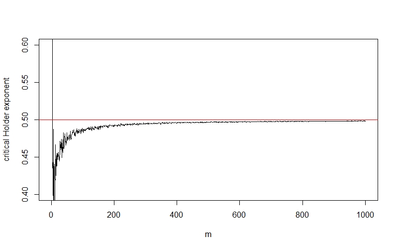
(a) Brownian motion

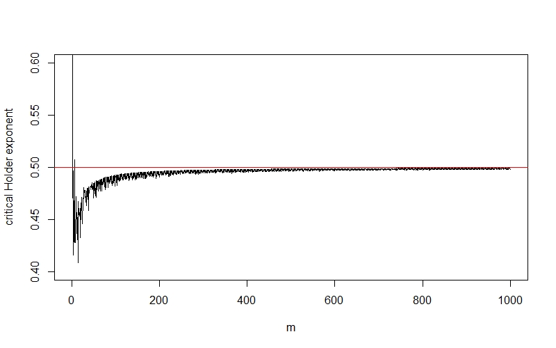
(b) Fake Brownian motion

Figure 1: Estimating Hölder regularity

In Figure 1, we plot the quantities $\displaystyle\max_{k}\frac{\log|\theta_{m,k}|}{\log|\pi^{m+1}|}$ for different values of $\displaystyle m$, where $\displaystyle(\theta_{m,k})$ are respective Schauder coefficients of Brownian motion and its fake version along the dyadic partition sequence on $\displaystyle[0,1]$ (for more details on the process faking BM, see Example 5). We leave further properties of the new Hölder estimator, such as convergence rate, as future work.

4 Critical Hölder exponent and variation index

Because the Hölder regularity is a local property, a given continuous function can have a different Hölder exponent over disjoint intervals (e.g. [11] provides a method of constructing a function with given local Hölder regularity). In particular, if we ‘patch’ a standard Brownian motion $\displaystyle B$ and a fractional Brownian motion $\displaystyle B^{H}$ with Hurst index $\displaystyle H=1/4$ over two intervals to define

$$Y(t):=B(t)\mathbbm{1}_{[0,1]}+\big{(}B^{H}(t-1)+B(1)\big{)}\mathbbm{1}_{(1,2]},\qquad t\in[0,2],$$

then we have $\displaystyle Y\in C^{\frac{1}{4}-}([0,2],\mathbb{R})$, but $\displaystyle Y\in C^{\frac{1}{2}-}([0,1],\mathbb{R})$. Thus, we shall consider the following concept of uniform Hölder property.

Definition 4.1 (Critical Hölder exponent and uniform Hölder).

For any $\displaystyle 0\leq t_{1}<t_{2}\leq T$, we define critical Hölder exponent of $\displaystyle x\in C^{0}([0,T],\mathbb{R})$ over $\displaystyle[t_{1},t_{2}]$

$$c(x,[t_{1},t_{2}]):=\sup_{0<\alpha\leq 1}\Big{\{}x\in C^{\alpha}([t_{1},t_{2}],\mathbb{R})\Big{\}}.$$ (21)

We say that $\displaystyle x$ is uniform Hölder over $\displaystyle[0,T]$, if $\displaystyle c(x,[t_{1},t_{2}])$ is the same for any two points $\displaystyle t_{1},t_{2}\in[0,T]$ with $\displaystyle t_{1}<t_{2}$.

For any $\displaystyle 0<\beta\leq 1$ and $\displaystyle 0\leq t_{1}<t_{2}\leq T$, it is obvious from the definition (21) that we have

$$\displaystyle\|x\|_{C^{\beta}([t_{1},t_{2}])}=\begin{cases}\infty,&\beta>c(x,[t_{1},t_{2}]),\\ \,0,&\beta<c(x,[t_{1},t_{2}]).\end{cases}$$

Proposition 4.2.

We have an alternative representation of the critical Hölder exponent:

$$\tilde{c}(x,[t_{1},t_{2}]):=\sup_{0<\alpha\leq 1}\Big{\{}\limsup_{h\downarrow 0}\sup_{t_{1}\leq s\leq t_{2}-h}\frac{|x(s+h)-x(s)|}{|h|^{\alpha}}<\infty\Big{\}}$$

satifies $\displaystyle c(x,[t_{1},t_{2}])=\tilde{c}(x,[t_{1},t_{2}])$ for every $\displaystyle x\in C^{0}([0,T],\mathbb{R})$ and $\displaystyle 0\leq t_{1}<t_{2}\leq T$.

Proof.

For fixed $\displaystyle 0\leq t_{1}<t_{2}\leq T$, we write

$$A_{\alpha}:=\|x\|_{C^{\alpha}([t_{1},t_{2}])}=\sup_{\begin{subarray}{c}u,v\in[t_{1},t_{2}]\\ u\neq v\end{subarray}}\frac{|x(u)-x(v)|}{|u-v|^{\alpha}},\qquad B_{\alpha}:=\limsup_{h\downarrow 0}\sup_{t_{1}\leq s\leq t_{2}-h}\frac{|x(s+h)-x(s)|}{|h|^{\alpha}},$$

then we obviously have $\displaystyle A_{\alpha}\geq B_{\alpha}$, which implies $\displaystyle c(x,[t_{1},t_{2}])\leq\tilde{c}(x,[t_{1},t_{2}])$ from the definition (21).

In order to show the reversed inequality, we first claim that $\displaystyle A_{\alpha}=\infty$ implies $\displaystyle B_{\alpha}=\infty$ in the following. Let us assume $\displaystyle A_{\alpha}=\infty$, but $\displaystyle B_{\alpha}=L<\infty$. Then, there exists a positive constant $\displaystyle\delta$ such that

$$\sup_{t_{1}\leq s\leq t_{2}-h}\frac{|x(s+h)-x(s)|}{|h|^{\alpha}}\leq L+1$$ (22)

for every positive $\displaystyle h$ satisfying $\displaystyle h<\delta$. On the other hand, from the assumption $\displaystyle A_{\alpha}=\infty$, there exist two sequences $\displaystyle\{u_{n}\}_{n\in\mathbb{N}}$ and $\displaystyle\{v_{n}\}_{n\in\mathbb{N}}$ on $\displaystyle[t_{1},t_{2}]$ such that $\displaystyle u_{n}\neq v_{n}$ and

$$\frac{|x(u_{n})-x(v_{n})|}{|u_{n}-v_{n}|^{\alpha}}>n$$

holds for every $\displaystyle n\in\mathbb{N}$. In particular, for every integer $\displaystyle n$ greater than $\displaystyle\max\{L+2,2M/{\delta}^{\alpha}\}$ with the notation $\displaystyle M:=\sup\{s\in[t_{1},t_{2}]:|x(s)|\}<\infty$, we have $\displaystyle|u_{n}-v_{n}|\geq\delta$ from (22). Then, we have the estimates

$$\frac{|x(u_{n})-x(v_{n})|}{|u_{n}-v_{n}|^{\alpha}}\leq\frac{2M}{|u_{n}-v_{n}|^{\alpha}}\leq\frac{2M}{\delta^{\alpha}}\leq n,$$

which contradicts the previous inequality. This proves the claim and we derive the series of equivalences

$$\displaystyle\big{(}A_{\alpha}=\infty\implies B_{\alpha}=\infty\big{)}\quad \displaystyle\iff\quad\big{(}B_{\alpha}<\infty\implies A_{\alpha}<\infty\big{)}$$

$$\displaystyle\iff\quad\sup_{0<\alpha\leq 1}\{A_{\alpha}<\infty\}\geq\sup_{0<\alpha\leq 1}\{B_{\alpha}<\infty\}\quad \displaystyle\iff\quad c(x,[t_{1},t_{2}])\geq\tilde{c}(x,[t_{1},t_{2}]),$$

which completes the proof. ∎

We now give a concept of $\displaystyle p$-th variation of $\displaystyle x\in C^{0}([0,T],\mathbb{R})$ along a given refining sequence $\displaystyle\pi$ with vanishing mesh. This definition is from Definition 1.1 and Lemma 1.3 of [10].

Definition 4.3 ($\displaystyle p$-th variation along a partition sequence $\displaystyle\pi$).

For a given refining sequence $\displaystyle\pi$ of partitions of $\displaystyle[0,T]$ with vanishing mesh and a continuous function $\displaystyle x\in C^{0}([0,T],\mathbb{R})$, if there exists a continuous function $\displaystyle[x]^{(p)}_{\pi}:[0,T]\rightarrow\mathbb{R}$ such that

$$\sum_{\begin{subarray}{c}t^{n}_{j},t^{n}_{j+1}\in\pi^{n}\\ t^{n}_{j}\leq t\end{subarray}}\Big{|}x(t^{n}_{j+1})-x(t^{n}_{j})\Big{|}^{p}\xlongrightarrow{n\rightarrow\infty}[x]^{(p)}_{\pi}(t)\quad\text{uniformly in }t,$$ (23)

then we say $\displaystyle x$ has finite $\displaystyle p$-th variation along $\displaystyle\pi$, and call $\displaystyle[x]^{(p)}_{\pi}$ the $\displaystyle p$-th variation of $\displaystyle x$ along $\displaystyle\pi$. We denote $\displaystyle V^{p}_{\pi}([0,T],\mathbb{R})$ the set of all continuous functions with finite $\displaystyle p$-th variation along $\displaystyle\pi$.

For $\displaystyle p=2$, the class $\displaystyle V^{2}_{\pi}([0,T],\mathbb{R})$ is identified as a set of functions with finite quadratic variation along $\displaystyle\pi$, in the sense of [14], and often denoted by $\displaystyle Q_{\pi}([0,T],\mathbb{R})$ instead of $\displaystyle V^{2}_{\pi}([0,T],\mathbb{R})$. Even though the $\displaystyle p$-th variation of $\displaystyle x$ along a given sequence $\displaystyle\pi$ may not exist, one can always define its variation index along $\displaystyle\pi$ as in [7].

Definition 4.4 (Variation index along a partition sequence).

The variation index of $\displaystyle x\in C^{0}([0,T],\mathbb{R})$ along a refining partition sequence $\displaystyle\pi$ with vanishing mesh is defined as

$$p^{\pi}(x):=\inf\bigg{\{}p\geq 1\,:\,\limsup_{n\uparrow\infty}\sum_{t^{n}_{i},t^{n}_{i+1}\in\pi^{n}}\Big{|}x(t^{n}_{i+1})-x(t^{n}_{i})\Big{|}^{p}=0\bigg{\}}.$$ (24)

It is straightforward to show

$$\limsup_{n\uparrow\infty}\sum_{t^{n}_{i},t^{n}_{i+1}\in\pi^{n}}\Big{|}x(t^{n}_{i+1})-x(t^{n}_{i})\Big{|}^{q}=\begin{cases}\,0,\qquad&q>p^{\pi}(x),\\ \infty,\qquad&q<p^{\pi}(x),\end{cases}$$

from the fact that the mesh size of $\displaystyle\pi^{n}$ converges to zero, together with the inequality

$$\displaystyle\sum_{t^{n}_{i},t^{n}_{i+1}\in\pi^{n}} \displaystyle\big{|}x(t^{n}_{i+1})-x(t^{n}_{i})\big{|}^{q}$$

$$\displaystyle\leq\bigg{(}\max_{t^{n}_{i},t^{n}_{i+1}\in\pi^{n}}\big{|}x(t^{n}_{t_{i+1}})-x^{n}(t_{i})\big{|}^{q-p^{\pi}(x)}\bigg{)}\bigg{(}\sum_{t^{n}_{i},t^{n}_{i+1}\in\pi^{n}}\big{|}x(t^{n}_{i+1})-x(t^{n}_{i})\big{|}^{p^{\pi}(x)}\bigg{)}.$$

Therefore, the definition (24) can be also formulated as

$$p^{\pi}(x)=\inf\bigg{\{}p\geq 1:\limsup_{n\uparrow\infty}\sum_{t^{n}_{i},t^{n}_{i+1}\in\pi^{n}}\Big{|}x(t^{n}_{i+1})-x(t^{n}_{i})\Big{|}^{p}<\infty\bigg{\}}.$$ (25)

We note that both $\displaystyle[x]^{(p)}_{\pi}$ and $\displaystyle p^{\pi}(x)$ depend not only on $\displaystyle x$ but also on the sequence $\displaystyle\pi$ of partitions.

On the contrary, for a given continuous function $\displaystyle x\in C^{0}([0,T],\mathbb{R})$, the rough path theory defines the $\displaystyle p$-variation of $\displaystyle x$ by taking the supremum of $\displaystyle p$ variations over all partitions of $\displaystyle[0,T]$:

$$\|x\|_{p-var}:=\bigg{(}\sup_{\pi\in\Pi([0,T])}\sum_{t_{j},t_{j+1}\in\pi}\big{|}x(t_{j+1})-x(t_{j})\big{|}^{p}\bigg{)}^{1/p},$$

where $\displaystyle\Pi([0,T])$ denotes the set of all partitions of $\displaystyle[0,T]$. The quantity $\displaystyle\|x\|_{p-var}$ is then partition-independent and the relationship

$$\Big{(}\|x\|_{p-var}\Big{)}^{p}\geq\limsup_{n\uparrow\infty}\sum_{t^{n}_{i},t^{n}_{i+1}\in\pi^{n}}\Big{|}x(t^{n}_{i+1})-x(t^{n}_{i})\Big{|}^{p}$$ (26)

easily follows for any refining sequence $\displaystyle\pi$ with vanishing mesh.

Lemma 4.5.

For any $\displaystyle x\in C^{\alpha}([0,T],\mathbb{R})$, $\displaystyle x$ has finite $\displaystyle\frac{1}{\alpha}$-variation, i.e., $\displaystyle\|x\|_{\frac{1}{\alpha}-var}<\infty$. Furthermore, for every refining sequence $\displaystyle\pi$ of partitions on $\displaystyle[0,T]$ with vanishing mesh, we have the inequality

$$\frac{1}{p^{\pi}(x)}\geq c(x,[0,T]).$$ (27)

Proof.

For an arbitrary partition $\displaystyle\pi\in\Pi([0,T])$, the $\displaystyle\alpha$-Hölder continuity of $\displaystyle x$ yields

$$\displaystyle\sum_{t_{j},t_{j+1}\in\pi}\big{|}x(t_{j+1})-x(t_{j})\big{|}^{p} \displaystyle\leq\sum_{t_{j},t_{j+1}\in\pi}\bigg{(}\|x\|_{C^{\alpha}([0,T])}\big{|}x(t_{j+1})-x(t_{j})\big{|}^{\alpha}\bigg{)}^{p}$$

$$\displaystyle=\Big{(}\|x\|_{C^{\alpha}([0,T])}\Big{)}^{p}\bigg{(}\sum_{t_{j},t_{j+1}\in\pi}|t_{j+1}-t_{j}|^{\alpha p}\bigg{)}$$

$$\displaystyle=T\Big{(}\|x\|_{C^{\alpha}([0,T])}\Big{)}^{p}<\infty,$$

where the last equality holds if $\displaystyle p=\frac{1}{\alpha}$. This proves $\displaystyle\|x\|_{\frac{1}{\alpha}-var}<\infty$, which in turn implies

$$\limsup_{n\uparrow\infty}\sum_{t^{n}_{i},t^{n}_{i+1}\in\pi^{n}}\Big{|}x(t^{n}_{i+1})-x(t^{n}_{i})\Big{|}^{\frac{1}{\alpha}}<\infty$$ (28)

for any refining sequence $\displaystyle\pi$ of vanishing mesh from (26).

Now that $\displaystyle\|x\|_{C^{\alpha}([0,T])}<\infty$ implies (28), the definitions (21) and (25) conclude

$$c(x,[0,T])=\sup_{0<\alpha\leq 1}\Big{\{}\|x\|_{C^{\alpha}([0,T])}<\infty\Big{\}}\leq\frac{1}{p^{\pi}(x)}.$$

∎

Even though the critical Hölder exponent and the reciprocal of variation index are the same for fractional Brownian motions along any partition sequence with mesh size converging to zero fast enough (as a result of self-similarity), they are not the same for general processes. The following provides an example of a deterministic function with critical Hölder exponent different from the reciprocal of variation index.

Example 1 (A function with different critical Hölder exponent and reciprocal of variation index).

For a fixed $\displaystyle 0<\epsilon_{0}<\frac{1}{3}$, consider a function $\displaystyle x:[0,1]\rightarrow\mathbb{R}$ given by the Schauder representation along the dyadic partition $\displaystyle\mathbb{T}$

$$x(t)=\sum_{m=0}^{\infty}\sum_{k\in I_{m}}\theta_{m,k}e^{\mathbb{T}}_{m,k}(t),$$ (29)

where the Schauder coefficients are given by

$$\displaystyle\theta_{m,k}=\begin{cases}2^{\epsilon_{0}m},&k=0,\,\left\lfloor\frac{2^{m}}{\sqrt[4]{m}}\right\rfloor\wedge(2^{m}-1),\,2\left\lfloor\frac{2^{m}}{\sqrt[4]{m}}\right\rfloor\wedge(2^{m}-1),\cdots\\ 0,&\text{otherwise}.\end{cases}$$

Then, the function $\displaystyle x$ is continuous and we have the strict inequality for this pair $\displaystyle(x,\mathbb{T})$

$$\frac{1}{p^{\mathbb{T}}(x)}>c(x,[0,1]).$$

∎

Proof.

Lemma 2.10(iii) implies that $\displaystyle x$ is continuous.

We will show that $\displaystyle c(x,[0,T])=\frac{1}{2}-\epsilon_{0}$. It is easy to verify

$$\sup_{m,k}\big{(}|\theta_{m,k}|\times 2^{m(\alpha-\frac{1}{2})}\big{)}=\sup_{m,k}\big{(}2^{(\epsilon_{0}+\alpha-\frac{1}{2})m}\big{)}=\begin{cases}0,\qquad&\alpha<\frac{1}{2}-\epsilon_{0},\\ 1,\qquad&\alpha=\frac{1}{2}-\epsilon_{0},\\ \infty,\qquad&\alpha>\frac{1}{2}-\epsilon_{0},\end{cases}$$

thus, Theorem 3.4 implies $\displaystyle x\in C^{\alpha}([0,1],\mathbb{R})$ for every $\displaystyle\alpha\leq\frac{1}{2}-\epsilon_{0}$. From the definition of critical exponent this implies $\displaystyle c(x,[0,1])=\frac{1}{2}-\epsilon_{0}$. Now we will show that $\displaystyle x\in Q_{\mathbb{T}}([0,1],\mathbb{R})$. Quadratic variation at level $\displaystyle n$ can be represented with the Schauder coefficients from Proposition 4.1 of [8]:

$$\displaystyle[x]^{(2)}_{\mathbb{T}^{n}}(1) \displaystyle=\frac{1}{2^{n}}\sum_{m=0}^{n-1}\sum_{k=0}^{2^{m}-1}\theta_{m,k}^{2}=\frac{1}{2^{n}}\sum_{m=0}^{n-1}2^{2\epsilon_{0}m}\times\lfloor\sqrt[4]{m}\rfloor\leq\frac{1}{2^{n}}\sum_{m=0}^{n-1}2^{2\epsilon_{0}m+\frac{1}{4}log_{2}m}$$

$$\displaystyle\leq\frac{1}{2^{n}}\sum_{m=0}^{n-1}2^{(2\epsilon_{0}+\frac{1}{4})m}=\frac{1}{2^{n}}\cdot\frac{2^{(2\epsilon_{0}+\frac{1}{4})n}-1}{2^{2\epsilon_{0}+\frac{1}{4}}-1}\xrightarrow[]{n\to\infty}0.$$

The last limit follows from the fact that $\displaystyle\epsilon_{0}<\frac{1}{3}$ implies $\displaystyle(2\epsilon_{0}+\frac{1}{4})-1<0$. Therefore, we have $\displaystyle x\in Q_{\mathbb{T}}([0,1],\mathbb{R})$ with $\displaystyle[x]^{(2)}_{\mathbb{T}}(1)=0$. From the definition of the variation index, we have $\displaystyle p^{\mathbb{T}}(x)\leq 2$ which implies $\displaystyle\frac{1}{p^{\mathbb{T}}(x)}\geq\frac{1}{2}>\frac{1}{2}-\epsilon_{0}=c(x,[0,1])$. This concludes the proof. ∎

The $\displaystyle p$-th variation of (a sample path of) a stochastic process along a given sequence of partitions and Hölder exponent are often used as an important tool to identify the Hurst index of a fractional Gaussian process. The following example shows one can construct a deterministic function which has the same ‘roughness’ order as Brownian motion but does not possess a Gaussian structure.

Example 2 (A function having the same path properties as Brownian motion).

We consider the dyadic partition $\displaystyle\mathbb{T}$ of $\displaystyle[0,1]$ and $\displaystyle x:[0,1]\rightarrow\mathbb{R}$ with the representation

$$x(t)=\sum_{m=0}^{\infty}\sum_{k\in I_{m}}\theta_{m,k}e^{\mathbb{T}}_{m,k}(t),$$ (30)

where the Schauder coefficients are given by

$$\displaystyle\theta_{m,k}=\begin{cases}\sqrt{m},&k=0,m,2m,\cdots,\lfloor\frac{2^{m}-1}{m}\rfloor m,\\ ~{}~{}0,&\text{otherwise}.\end{cases}$$

Then, $\displaystyle x\in C^{0}([0,1],\mathbb{R})$, $\displaystyle x$ is uniform Hölder, $\displaystyle\|x\|_{C^{1/2}([0,1])}=\infty$, and $\displaystyle[x]^{(2)}_{\mathbb{T}}(t)=t$ for any $\displaystyle t\in[0,1]$. Almost every path of standard Brownian motion has these properties. ∎

Proof.

The continuity of $\displaystyle x$ is straightforward from Lemma 2.10(iii).

Since we have $\displaystyle\sup_{m,k}(|\theta_{m,k}||\pi^{m+1}|^{\frac{1}{2}-\alpha})=\sup_{m}(\sqrt{m}\times 2^{(m+1)(\alpha-\frac{1}{2})})$, this quantity is infinity when $\displaystyle\alpha=\frac{1}{2}$. Hence, Theorem 3.4 concludes $\displaystyle\|x\|_{C^{1/2}([0,1])}=\infty$. A similar argument shows that $\displaystyle\sup_{m,k}(|\theta_{m,k}||\pi^{m+1}|^{\frac{1}{2}-\alpha})<\infty$, hence $\displaystyle\|x\|_{C^{\alpha}([0,1])}<\infty$, if $\displaystyle\alpha<\frac{1}{2}$.

We now show that the quadratic variation of $\displaystyle x$ along $\displaystyle\mathbb{T}$ exists and is strictly positive. For a fixed $\displaystyle t\in(0,1]$, the quadratic variation up to level $\displaystyle n$ can be represented in terms of the Schauder coefficients from Proposition 4.1 of [8]:

$$\displaystyle[x]^{(2)}_{\mathbb{T}^{n}}(t)=\frac{1}{2^{n}}\sum_{m=0}^{n-1}\sum_{k=0}^{2^{m}-1}\theta_{m,k}^{2}\mathbbm{1}_{\frac{k}{2^{m}}<t} \displaystyle=\frac{1}{2^{n}}\sum_{m=0}^{n-1}\sum_{k=0}^{\lceil t2^{m}\rceil-1}\theta_{m,k}^{2}$$ (31)

$$\displaystyle=\frac{1}{2^{n}}\sum_{m=0}^{n-1}m\times\frac{\lceil t2^{m}\rceil}{2^{m}}\Big{(}\lfloor\frac{2^{m}-1}{m}\rfloor+1\Big{)}.$$

Using the equalities $\displaystyle 2^{m}-m-1<m\lfloor\frac{2^{m}-1}{m}\rfloor\leq 2^{m}-1$ and $\displaystyle t\leq\frac{\lceil t2^{m}\rceil}{2^{m}}<\frac{2^{m}t+1}{2^{m}}$, we obtain from (31) the following two-sided bounds on $\displaystyle[x]^{(2)}_{\mathbb{T}^{n}}(t)$

$$\displaystyle\frac{1}{2^{n}}\sum_{m=0}^{n-1}t(2^{m}-1)< \displaystyle[x]^{(2)}_{\mathbb{T}^{n}}(t)<\frac{1}{2^{n}}\sum_{m=0}^{n-1}(t+\frac{1}{2^{m}})(2^{m}+m-1)$$

$$\displaystyle\Rightarrow t\frac{1}{2^{n}}(2^{n}-1-n)< \displaystyle[x]^{(2)}_{\mathbb{T}^{n}}(t)<t\frac{1}{2^{n}}\Big{(}2^{n}-1+\frac{(n-1)n}{2}-n\Big{)}+\frac{2n}{2^{n}}.$$

Taking limit $\displaystyle n\to\infty$, we conclude $\displaystyle[x]^{(2)}_{\mathbb{T}}(t)=t>0$, i.e., $\displaystyle x$ has non-trivial quadratic variation along $\displaystyle\mathbb{T}$.

Finally, we show that the function $\displaystyle x$ is uniform Hölder. If we can show that for all $\displaystyle 0\leq t_{1}<t_{2}\leq 1$,

$$\sup_{u,v\in[0,1],u\neq v}\frac{|x(u)-x(v)|}{|u-v|^{\alpha}}<\infty\;\iff\;\sup_{u,v\in[t_{1},t_{2}],u\neq v}\frac{|x(u)-x(v)|}{|u-v|^{\alpha}}<\infty,$$

then from the definition of critical Hölder exponent, $\displaystyle x$ will be uniform Hölder (note that this condition is a sufficient condition but not a necessary condition). From the first part of the proof, we have

$$\sup_{u,v\in[0,1],u\neq v}\frac{|x(u)-x(v)|}{|u-v|^{\alpha}}<\infty\iff\alpha<\frac{1}{2},$$

thus in order to complete the proof, we only need to show that for $\displaystyle\alpha<\frac{1}{2}$

$$\sup_{u,v\in[t_{1},t_{2}],u\neq v}\frac{|x(u)-x(v)|}{|u-v|^{\alpha}}<\infty.$$

We choose large enough $\displaystyle n_{0}\in\mathbb{N}$ such that $\displaystyle\frac{1}{2^{n_{0}}}<|t_{2}-t_{1}|$. Then, we have $\displaystyle\sup_{k}|\theta_{n,k}|\mathbbm{1}_{[t_{1},t_{2}]}=\sqrt{n}$ for all $\displaystyle n\geq n_{0}$. Finally, we have for all $\displaystyle\alpha<\frac{1}{2}$

$$\sup_{m,k}\Big{(}|\theta_{m,k}||\pi^{m+1}|^{\frac{1}{2}-\alpha}\Big{)}\mathbbm{1}_{[t_{1},t_{2}]}=\sup_{m}\Big{(}\sqrt{m}\times 2^{(m+1)(\alpha-\frac{1}{2})}\Big{)}<\infty.$$

Similarly, for $\displaystyle\alpha>\frac{1}{2}$, we have $\displaystyle\sup_{m,k}(|\theta_{m,k}||\pi^{m+1}|^{\frac{1}{2}-\alpha})\mathbbm{1}_{[t_{1},t_{2}]}=\infty$. This concludes that $\displaystyle x$ is indeed uniform Hölder. ∎

Remark 4.6.

Even though we construct deterministic functions with certain path properties in Examples 1 and 2, we can transform them into stochastic processes by making the Schauder coefficients random. For example, consider a sequence of Bernoulli random variables $\displaystyle\{\beta_{m,k}\}$ with $\displaystyle\beta_{m,k}\sim Bernoulli(1/2)$ (these random variables $\displaystyle\beta_{m,k}$ do not need to be independent), replace the deterministic coefficients $\displaystyle\theta_{m,k}$ with the random coefficients $\displaystyle\theta_{m,k}\beta_{m,k}$ in the representations (29) and (30), respectively, and denote the resulting process by $\displaystyle Y$. Then, the above arguments can be applied to show that almost every path of the stochastic process $\displaystyle Y$ has the same properties as in Examples 1 and 2, respectively.

Figure 2 illustrates a deterministic function $\displaystyle t\mapsto x(t)$ in Example 2 and a sample path of the corresponding process $\displaystyle Y$ mentioned in Remark 4.6, together with their quadratic variations along the dyadic partitions.

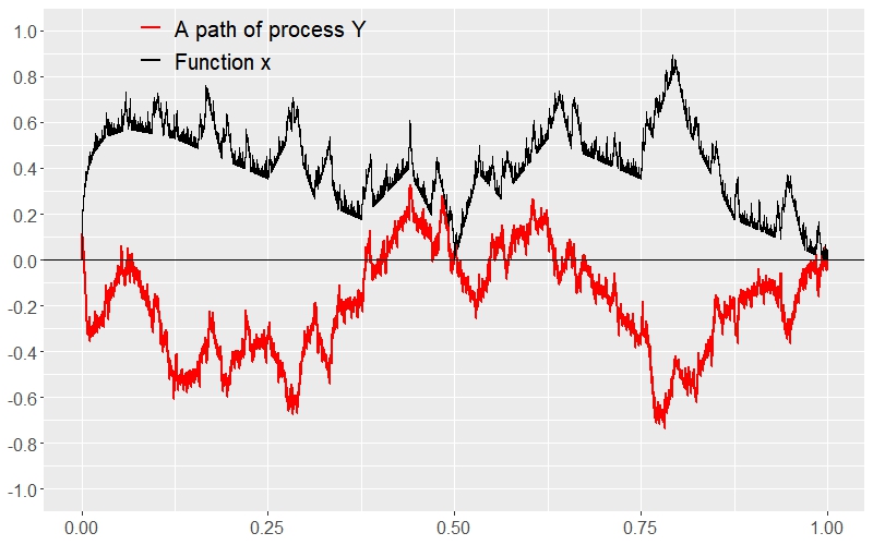
(a) Function $\displaystyle x$ and a sample path of $\displaystyle Y$

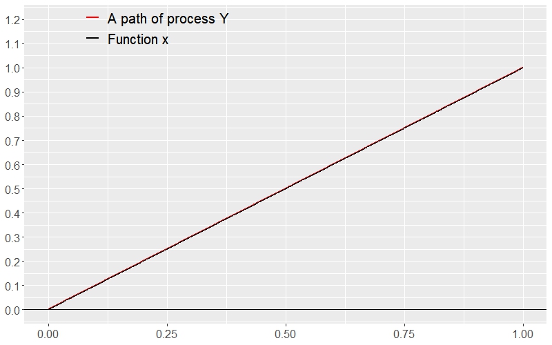
(b) Quadratic variations

Figure 2: Function $\displaystyle x$, a sample path of $\displaystyle Y$, and their quadratic variations in Example 2, truncated at level $\displaystyle n=16$.

5 Fake Brownian motion

In this section, we construct stochastic processes which fake Brownian motion using the Schauder representation. For a finitely refining sequence $\displaystyle\pi$ of partitions of $\displaystyle[0,1]$, we have the following Schauder representation of a Brownian motion $\displaystyle B$ along $\displaystyle\pi$, due to Proposition 2.9 (or more precisely Lemma 5.1 of [8]):

$$B(t)=Zt+\sum_{m=0}^{\infty}\sum_{k\in I_{m}}\theta_{m,k}^{B}e^{\pi}_{m,k}(t),\qquad t\in[0,1],$$ (32)

where $\displaystyle Z=B(1)$ and the coefficients $\displaystyle\theta^{B}_{m,k}$ are independent and identically distributed standard normal random variables.

We shall construct non-Gaussian processes, which have many properties in common with Brownian motion by replacing the normal Schauder coefficients $\displaystyle\theta^{B}_{m,k}$ with some non-normal random variables. Furthermore, we shall show that these non-Gaussian processes even ‘mimic’ the normality; many classical normality tests conclude that these fake processes have Gaussian marginal distributions despite being theoretically non-Gaussian.

5.1 Construction of fake Brownian processes

We shall focus on the construction of fake processes on the interval $\displaystyle[0,1]$, as Remark 5.3 below explains how the construction method can be extended to the entire non-negative real line $\displaystyle[0,\infty)$.

The following theorem provides a list of properties (BM i - vii) of Brownian motion $\displaystyle B$ in (32) we shall fake.

Theorem 5.1 (Construction of fake Brownian motion).

For a balanced and complete refining sequence of partition $\displaystyle\pi$ of $\displaystyle[0,1]$, consider the stochastic process $\displaystyle Y$ defined on $\displaystyle[0,1]$ via Schauder representation along $\displaystyle\pi$

$$Y(t)=Zt+\sum_{m=0}^{\infty}\sum_{k\in I_{m}}\theta^{Y}_{m,k}e^{\pi}_{m,k}(t),$$

where $\displaystyle\{\theta_{m,k}^{Y}\}$ are independent random variables satisfying

1. $\displaystyle\mathbb{E}[\theta^{Y}_{m,k}]=0$ and $\displaystyle Var[\theta^{Y}_{m,k}]=1$,

2. there exist positive constants $\displaystyle C_{1}$ and $\displaystyle C_{2}$ such that

   $$\mathbb{P}\big{[}|\theta^{Y}_{m,k}|\geq\delta\big{]}\leq C_{1}\exp\bigg{(}-\frac{{\delta}^{2}}{2C_{2}}\bigg{)}$$

   holds for every $\displaystyle\delta>0$, $\displaystyle k\in I_{m}$, $\displaystyle m\geq 0$.

Then, the process $\displaystyle Y$ satisfies the following properties (BM i-vii).

1. $\displaystyle Y$ has a continuous path almost surely.

2. $\displaystyle\mathbb{E}[Y(t)]=0$ and $\displaystyle\mathbb{E}[Y(t)Y(s)]=t\wedge s$ for any $\displaystyle t,s\in[0,1]$.

3. Increments of $\displaystyle Y$ over disjoint intervals are uncorrelated, i.e.,
   $\displaystyle\mathbb{E}[(Y(t)-Y(s))(Y(v)-Y(u))]=0$ for every $\displaystyle 0\leq s\leq t\leq u\leq v\leq 1$.

4. Almost every path of $\displaystyle Y$ belongs to $\displaystyle C^{\frac{1}{2}-}([0,T],\mathbb{R})$.

5. The Schauder coefficients $\displaystyle\theta_{m,k}^{Y}$ have mean $\displaystyle 0$, variance $\displaystyle 1$, and are uncorrelated, i.e., $\displaystyle\mathbb{E}(\theta_{m,k}^{Y})=0,\text{Var}(\theta_{m,k}^{Y})=1$ and $\displaystyle\mathbb{E}(\theta_{m,k}^{Y}\theta_{m^{\prime},k}^{Y})=\mathbbm{1}_{m=m^{\prime}}\mathbbm{1}_{k=k^{\prime}}$.

Moreover, in addition to (a) and (b), if we further assume the condition

1. $\displaystyle\mathbb{E}[(\theta^{Y}_{m,k})^{4}]<\infty$ for every $\displaystyle k\in I_{m}$, $\displaystyle m\geq 0$,

then, the process $\displaystyle Y$ satisfies the following additional properties

1. The quadratic variation along $\displaystyle\pi$ is given as $\displaystyle[Y]^{(2)}_{\pi}(t)=t$ for every $\displaystyle t\in[0,1]$ almost surely.

2. The quadratic variation along any coarsening partition $\displaystyle\nu$ of $\displaystyle\pi$ (see Definition 6.1 of [8] for further details on coarsening) is given as $\displaystyle[Y]^{(2)}_{\nu}(t)=t$ for every $\displaystyle t\in[0,1]$ almost surely.

The proofs of Theorem 5.1 and Remark 5.2 below will be given in Section 8.

Remark 5.2.

Property (BM iv) can be strengthened as the following under an additional assumption on the Schauder coefficients. If all random variables $\displaystyle(\theta^{Y}_{m,k})$ have the same bounded support such that

$$\mathbb{P}\Big{[}\sup_{m,k}|\theta^{Y}_{m,k}(\omega)|\leq C\Big{]}=1$$

holds for some constant $\displaystyle C>0$, then $\displaystyle Y$ of Theorem 5.1 satisfies

(BM iv’) Almost every path of $\displaystyle Y$ has the critical Hölder exponent $\displaystyle 1/2$.

We note that the fake process $\displaystyle Y$ in Theorem 5.1 cannot be a martingale (for any filtration) unless Brownian motion. If it were a martingale, then it is continuous from (BM i), square-integrable, i.e., $\displaystyle\mathbb{E}[(Y(t))^{2}]=t<\infty$ from (BM ii), and Theorem 1.5.13 of [24] yields the existence of a unique (up to indistinguishability) continuous process $\displaystyle\langle Y\rangle_{t}$ such that $\displaystyle Y^{2}_{t}-\langle Y\rangle_{t}$ is a martingale. Moreover, Theorem 1.5.8 of [24] and (BM vi) conclude that $\displaystyle\langle Y\rangle_{t}=[Y]^{(2)}_{\pi}(t)=t$ holds almost surely for every $\displaystyle t\in[0,1]$. The continuity of $\displaystyle t\mapsto\langle Y\rangle_{t}$ yields that the process $\displaystyle\langle Y\rangle_{t}$ is indistinguishable from $\displaystyle t$ and Lévy’s characterization of Brownian motion concludes that $\displaystyle Y$ should be a Brownian motion, which is a contradiction.

Remark 5.3 (fake Brownian motion on $\displaystyle[0,\infty)$).

Our construction method of fake Brownian motion in this subsection can be extended to the interval $\displaystyle[0,\infty)$ as Brownian motion has independent increments. Using the construction, we can define a sequence of independent fake Brownian motions $\displaystyle Y^{(i)}$ on intervals $\displaystyle[i-1,i]$ for $\displaystyle i=1,2,\cdots$ and patch them recursively by

$$\displaystyle Y_{t}:=Y^{(1)}(t),\qquad \displaystyle 0\leq t\leq 1,$$

$$\displaystyle Y_{t}:=Y_{n}+Y^{(n+1)}_{t-n},\qquad \displaystyle n\leq t\leq n+1.$$

Then, the resulting process $\displaystyle Y$ has the same aforementioned properties as Brownian motion on $\displaystyle[0,\infty)$. See Corollary 2.3.4 of [24] for further details on this patching. However, this patching method does not work for fake-fBM in the next subsection, since the increments of fBM are correlated for all Hurst index $\displaystyle H\neq 1/2$.

5.2 Examples

We now provide a couple of fake processes that satisfy the conditions of Theorem 5.1.

Example 3 (Uniformly distributed coefficients).

Let us denote $\displaystyle U$ a uniformly distributed random variable over the interval $\displaystyle[-\sqrt{3},\,\sqrt{3}]$, i.e., $\displaystyle U\sim\text{Uniform}(-\sqrt{3},\,\sqrt{3})$ such that its mean and variance are zero and one respectively. For a given complete refining and balanced sequence $\displaystyle\pi$ of partitions of $\displaystyle[0,1]$, consider a process $\displaystyle Y$ on $\displaystyle[0,1]$ with the representation

$$Y(t)=Zt+\sum_{m=0}^{\infty}\sum_{k\in I_{m}}\theta^{Y}_{m,k}e^{\pi}_{m,k}(t),$$ (33)

where the Schauder coefficients $\displaystyle\theta^{Y}_{m,k}$ are independent and identically distributed as $\displaystyle U$ and $\displaystyle Z\sim N(0,1)$ independent of all the other Schauder coefficients. Then, from Theorem 5.1 the process $\displaystyle Y$ has properties (BM i - vii) as Brownian motion. ∎

Example 4 (Centred, scaled beta distributed coefficients).

Since the beta distribution is a family of continuous probability distributions with compact support which generalizes uniform distribution, we can use a beta distribution as the Schauder coefficients. For example, we consider two-centred, scaled beta distributed random variables

$$B_{1}\sim\sqrt{20}\Big{(}\text{Beta}(2,2)-\frac{1}{2}\Big{)},\qquad B_{2}\sim\sqrt{8}\Big{(}\text{Beta}(\frac{1}{2},\frac{1}{2})-\frac{1}{2}\Big{)},$$ (34)

such that both of them have mean zero and variance one. We construct two processes $\displaystyle Y_{1}$ and $\displaystyle Y_{2}$ on $\displaystyle[0,1]$ such that their Schauder coefficients $\displaystyle\theta^{Y_{i}}_{m,k}$ in the representation (33) are independent and identically distributed as $\displaystyle B_{i}$ of (34) for $\displaystyle i=1,2$. ∎

Figure 3 provides simulations of the processes $\displaystyle B(t)-Zt$ of (32), $\displaystyle Y-Zt$ in Example 3, and $\displaystyle Y_{i}-Zt$ in Example 4 for $\displaystyle i=1,2$, in black, red, blue, and green lines, respectively, along the dyadic partitions on $\displaystyle[0,1]$, up to level $\displaystyle n=15$. Note that these trajectories start at the origin and end at the point $\displaystyle(1,0)$. In order to have a trajectory of a real Brownian motion (and its fake versions), we can just add a linear term $\displaystyle Zt$ for some independent standard normal random variable $\displaystyle Z$, to those sample paths in Figure 3(a). Figure 3(b) shows that all paths indeed have the same quadratic variation as standard Brownian motion.

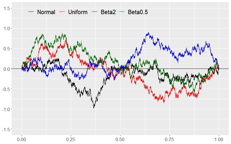
(a) Sample paths

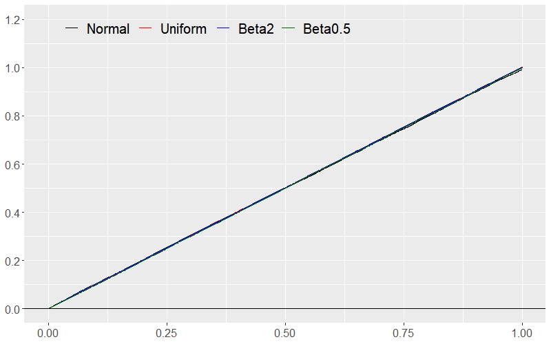
(b) Quadratic variations along dyadic paritions

Figure 3: Brownian process and its fake versions with different independent Schauder coefficients along dyadic partition sequence, truncated at level $\displaystyle n=15$.

Example 5 (Mixed coefficients).

To better fake Brownian motion, we can also mix standard normal random variables and other variables with the same mean and variance when choosing Schauder coefficients. For example, given the Schauder representation (33), we set the coefficients to be all independent, but distributed as

$$\theta^{Y_{mix}}_{m,k}\sim\begin{cases}\qquad N(0,1),\qquad&\text{if }m\text{ is odd},\\ \text{Uniform}(-\sqrt{3},\,\sqrt{3}),\qquad&\text{if }m\text{ is even}.\end{cases}$$ (35)

∎

Figure 4 describes this fake process and Section 5.3 provides normality test results for the marginal distributions of this process.

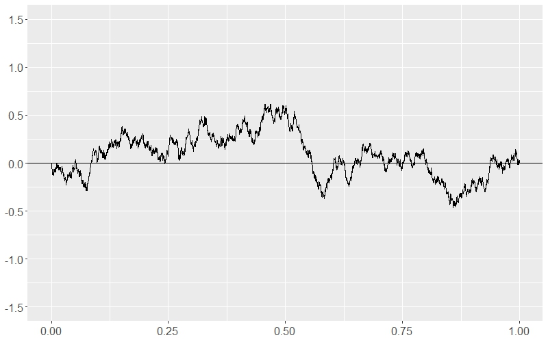
(a) A sample path

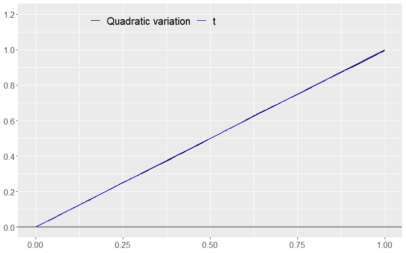
(b) Quadratic variation along dyadic paritions

Figure 4: Mixed version in Example 5 of fake process and its quadratic variation along dyadic partition sequence, truncated at level $\displaystyle n=15$.

Example 6 (Fake Brownian processes along a non-uniform partition).

Since the fake processes in Examples 3 - 5 were constructed along the same dyadic partitions, we introduce an example of a ‘non-uniform’ partition sequence. Define a sequence of partitions $\displaystyle\pi=(\pi^{n})_{n\in\mathbb{N}}$ with $\displaystyle\pi^{n}=\big{(}0=t^{n}_{1}<\cdots<t^{n}_{N(\pi_{n})}=1)$ satisfying

$$t^{n+1}_{2k}=t^{n}_{k},\qquad t^{n+1}_{2k+1}=t^{n}_{k}+\frac{t^{n}_{k+1}-t^{n}_{k}}{2.5},\qquad\forall\,k=1,\cdots,2^{n},$$

for each $\displaystyle n\in\mathbb{N}$. This sequence is still balanced and complete refining, thus we can construct the previous fake processes along this partition sequence. ∎

Figure 5 provides sample paths and corresponding quadratic variations of the fake processes in Example 3 - 5 along the non-uniform partition sequence in Example 6.

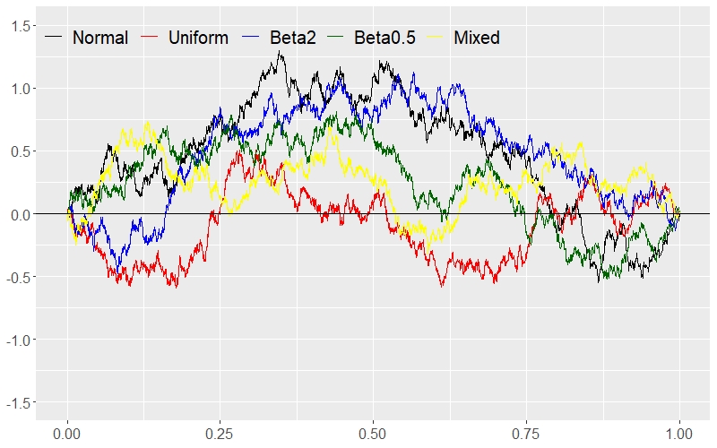
(a) Sample paths

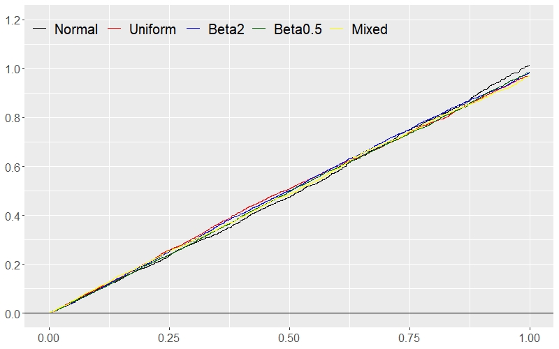
(b) Quadratic variations along non-uniform partition

Figure 5: Brownian process and its fake processes along the non-uniform doubly refining partition sequence, truncated at level $\displaystyle n=15$.

5.3 Normality tests on the marginal distributions: theory vs. reality

Since we replaced normally distributed Schauder coefficients of Brownian motion with other random coefficients, the fake processes we constructed in the previous subsection are non-Gaussian processes, even with the mixed coefficients in Example 5. In particular, the marginal distributions of these processes cannot be identified as any well-known distribution, even though the first two moments of the marginal distributions coincide with those of Brownian motion (property (BM ii) of Theorem 5.1). Nonetheless, it turns out in the following that those non-Gaussian processes can even mimic the ‘Gaussian’ property.

In this regard, we first simulated $\displaystyle 5000$ sample paths of the fake Brownian process $\displaystyle Y_{mix}$ in Example 5, defined on $\displaystyle[0,1]$ along the dyadic partitions, truncated to the level $\displaystyle n=15$. We randomly chose $\displaystyle 10$ dyadic points $\displaystyle t_{i}\in(0,1)$ (such that each $\displaystyle t_{i}$ is given as $\displaystyle k/2^{15}$ with $\displaystyle k\in\mathbb{Z}$) and took $\displaystyle 5000$ sample values $\displaystyle Y_{mix}(t_{i})$ at each $\displaystyle t_{i}$ for $\displaystyle i=1,\cdots,10$. Then, we did three different normality tests, namely Shapiro–Wilk test, Kolmogorov–Smirnov test, and Jarque–Bera test, to decide whether those $\displaystyle 5000$ sample values for each point $\displaystyle t_{i}$ are drawn from a Gaussian distribution.

Table 1: $\displaystyle p$-values of three normality tests for $\displaystyle 5000$ sample paths of the fake Brownian process $\displaystyle Y_{mix}$ at $\displaystyle 10$ randomly chosen dyadic points, truncated at level $\displaystyle n=15$.

point $\displaystyle t_{i}$	Shapiro-Wilk	Kolmogorov-Smirnov	Jarque-Bera
6653/$\displaystyle 2^{15}$	0.0980	0.9242	0.1350
5629/$\displaystyle 2^{15}$	0.1522	0.9472	0.3449
13835/$\displaystyle 2^{15}$	0.1342	0.8839	0.0388
30219/$\displaystyle 2^{15}$	0.0351	0.6151	0.0278
1032/$\displaystyle 2^{15}$	0.7342	0.9833	0.5482
103/$\displaystyle 2^{15}$	0.3448	0.4090	0.1591
14207/$\displaystyle 2^{15}$	0.4661	0.9793	0.4173
14469/$\displaystyle 2^{15}$	0.0583	0.5532	0.1943
2245/$\displaystyle 2^{15}$	0.6819	0.9089	0.2250
325/$\displaystyle 2^{15}$	0.3677	0.8564	0.3479

Table 1 provides the $\displaystyle p$-values of the three normality tests for $\displaystyle 10$ randomly chosen dyadic points. As we can observe, most of the $\displaystyle p$-values are bigger than $\displaystyle 5\%$, meaning we should not reject the null hypothesis (with a significance level of $\displaystyle 0.05$) stating that our sample values are drawn from a Gaussian distribution; the $\displaystyle p$-values which are less than $\displaystyle 5\%$ are displayed in boldface. Figure 6 also gives histograms and Q-Q plots of the $\displaystyle 5000$ sample values of $\displaystyle Y_{mix}(t)$ at another two (randomly chosen dyadic) points, $\displaystyle t=102/2^{15}$ and $\displaystyle 6653/2^{15}$.

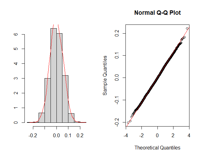
(a) $\displaystyle t=102/2^{15}$

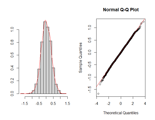
(b) $\displaystyle t=6653/2^{15}$

Figure 6: Histograms and Q-Q plots for $\displaystyle 5000$ sample points of $\displaystyle Y_{mix}$

Despite the marginal distributions of the fake Brownian process $\displaystyle Y_{mix}$ are not theoretically Gaussian, the above simulation study concludes that they are statistically Gaussian. In practice, when observing entire sample trajectories (or some discrete sample signals) drawn from an unknown process, we can check some path properties such as (BM i, iv, vi) and compute moments of marginals (BM ii, iii) to find out the distribution of the unknown process. However, our construction method suggests that it would be very hard to distinguish real Brownian motion from those non-Gaussian fake processes.

Remark 5.4 (faking higher order moments).

When constructing the fake fractional processes in Theorem 5.1, we only matched the first two moments of the Schauder coefficients as those of Brownian motion. Nevertheless, most of the $\displaystyle p$-values in Table 1 are quite big for the Jacque-Bera test, which is a goodness-of-fit test of whether sample data have the third and fourth moments (skewness and kurtosis) matching a normal distribution. If we want to further mimic those higher-order moments, we may choose random variables (other than $\displaystyle U\sim\text{Uniform}(-\sqrt{3},\sqrt{3})$) with the same moments up to higher-order as the standard normal distribution, for the Schauder coefficients, due to Theorem 7.1 later. For example, a discrete random variable

$$R\sim\begin{cases}&~{}~{}\sqrt{3},\qquad\text{with probability }1/6,\\ &-\sqrt{3},\qquad\text{with probability }1/6,\\ &~{}~{}~{}0,~{}~{}\qquad\text{with probability }2/3,\end{cases}$$

has the same first four moments with the standard normal distribution and satisfies the conditions of Theorem 5.1.

6 Fake fractional Brownian motions

A fractional Brownian motion (fBM) $\displaystyle B^{H}$, defined on $\displaystyle[0,1]$, with Hurst index $\displaystyle H\in(0,1)$ has the following Schauder representation along a finitely refining partition sequence $\displaystyle\pi$ from Proposition 2.9:

$$B^{H}(t)=Zt+\sum_{m=0}^{\infty}\sum_{k\in I_{m}}\theta^{B^{H}}_{m,k}e^{\pi}_{m,k}(t),\qquad t\in[0,1],$$ (36)

where $\displaystyle Z=B^{H}(1)$ and $\displaystyle\theta^{B^{H}}_{m,k}$ are normally distributed with mean zeros and variance equal to $\displaystyle 1$ and $\displaystyle\sigma^{2}_{m,k}$, respectively, with the notation

$$\sigma^{2}_{m,k}:=\frac{(\Delta^{m,k}_{2})^{2}(\Delta^{m,k}_{1})^{2H}+(\Delta^{m,k}_{1})^{2}(\Delta^{m,k}_{2})^{2H}-\Delta^{m,k}_{1}\Delta^{m,k}_{2}\Big{[}(\Delta^{m,k}_{1}+\Delta^{m,k}_{2})^{2H}-(\Delta^{m,k}_{1})^{2H}-(\Delta^{m,k}_{2})^{2H}\Big{]}}{\Delta^{m,k}_{1}\Delta^{m,k}_{2}(\Delta^{m,k}_{1}+\Delta^{m,k}_{2})}.$$ (37)

Here and in what follows, we shall denote

$$\Delta^{m,k}_{1}:=t^{m,k}_{2}-t^{m,k}_{1}\text{ and }\Delta^{m,k}_{2}:=t^{m,k}_{3}-t^{m,k}_{2},$$

where the support of $\displaystyle e^{\pi}_{m,k}$ is $\displaystyle[t^{m,k}_{1},t^{m,k}_{3}]$ and its maximum is attained at $\displaystyle t^{k,n}_{2}$. We shall also use the notations $\displaystyle B^{H}\{\Delta^{m,k}_{1}\}:=B^{H}(t^{m,k}_{2})-B^{H}(t^{m,k}_{1})$ and $\displaystyle B^{H}\{\Delta^{m,k}_{2}\}:=B^{H}(t^{m,k}_{3})-B^{H}(t^{m,k}_{2})$, with the similar notations for another pair of indices $\displaystyle m^{\prime}$ and $\displaystyle k^{\prime}$ and corresponding Schauder function $\displaystyle e^{\pi}_{m^{\prime},k^{\prime}}(.)$.

Since the increments of fBM are not independent (except for the case $\displaystyle H=1/2$), as a result the coefficients $\displaystyle\theta^{B^{H}}_{m,k}$ are not independent. Again from the expression (10), we can compute the covariance between two Schauder coefficients:

$$\displaystyle\sigma_{m,k,m^{\prime},k^{\prime}}:=\mathbb{E}[\theta^{B^{H}}_{m,k}\theta^{B^{H}}_{m^{\prime},k^{\prime}}]$$ (38)

$$\displaystyle=\frac{\Delta^{m,k}_{2}\Delta^{m^{\prime},k^{\prime}}_{2}\xi^{m,k,m^{\prime},k^{\prime}}_{1,1}+\Delta^{m,k}_{1}\Delta^{m^{\prime},k^{\prime}}_{1}\xi^{m,k,m^{\prime},k^{\prime}}_{2,2}-\Delta^{m,k}_{1}\Delta^{m^{\prime},k^{\prime}}_{2}\xi^{m,k,m^{\prime},k^{\prime}}_{2,1}-\Delta^{m^{\prime},k^{\prime}}_{1}\Delta^{m,k}_{2}\xi^{m,k,m^{\prime},k^{\prime}}_{1,2}}{\sqrt{\Delta^{m,k}_{1}\Delta^{m,k}_{2}\Delta^{m^{\prime},k^{\prime}}_{1}\Delta^{m^{\prime},k^{\prime}}_{2}(\Delta^{m,k}_{1}+\Delta^{m,k}_{2})(\Delta^{m^{\prime},k^{\prime}}_{1}+\Delta^{m^{\prime},k^{\prime}}_{2})}}$$

where

$$\displaystyle\xi^{m,k,m^{\prime},k^{\prime}}_{1,1} \displaystyle:=\mathbb{E}\big{[}B^{H}\{\Delta^{m,k}_{1}\}B^{H}\{\Delta^{m^{\prime},k^{\prime}}_{1}\}\big{]},\qquad\xi^{m,k,m^{\prime},k^{\prime}}_{2,2}:=\mathbb{E}\big{[}B^{H}\{\Delta^{m,k}_{2}\}B^{H}\{\Delta^{m^{\prime},k^{\prime}}_{2}\}\big{]},$$

$$\displaystyle\xi^{m,k,m^{\prime},k^{\prime}}_{2,1} \displaystyle:=\mathbb{E}\big{[}B^{H}\{\Delta^{m,k}_{2}\}B^{H}\{\Delta^{m^{\prime},k^{\prime}}_{1}\}\big{]},\qquad\xi^{m,k,m^{\prime},k^{\prime}}_{1,2}:=\mathbb{E}\big{[}B^{H}\{\Delta^{m,k}_{1}\}B^{H}\{\Delta^{m^{\prime},k^{\prime}}_{2}\}\big{]}.$$

Now that the covariance between the increments of fBM is given as

$$\displaystyle\quad 2\mathbb{E}\Big{[}\big{(}B^{H}(t)-B^{H}(s)\big{)}\big{(}B^{H}(v)-B^{H}(u)\big{)}\Big{]}$$

$$\displaystyle=\mathbb{E}\Big{[}\big{(}B^{H}(t)-B^{H}(u)\big{)}^{2}+\big{(}B^{H}(s)-B^{H}(v)\big{)}^{2}-\big{(}B^{H}(t)-B^{H}(v)\big{)}^{2}-\big{(}B^{H}(s)-B^{H}(u)\big{)}^{2}\Big{]}$$

$$\displaystyle=|t-u|^{2H}+|s-v|^{2H}-|t-v|^{2H}-|s-u|^{2H}$$

for any $\displaystyle s,t,u,v\in[0,1]$, we can derive the explicit expressions

$$\displaystyle\xi^{m,k,m^{\prime},k^{\prime}}_{1,1} \displaystyle=\frac{1}{2}\Big{(}|t^{m,k}_{1}-t^{m^{\prime},k^{\prime}}_{2}|^{2H}+|t^{m,k}_{2}-t^{m^{\prime},k^{\prime}}_{1}|^{2H}-|t^{m,k}_{1}-t^{m^{\prime},k^{\prime}}_{1}|^{2H}-|t^{m,k}_{2}-t^{m^{\prime},k^{\prime}}_{2}|^{2H}\Big{)},$$ (39)

$$\displaystyle\xi^{m,k,m^{\prime},k^{\prime}}_{2,2} \displaystyle=\frac{1}{2}\Big{(}|t^{m,k}_{2}-t^{m^{\prime},k^{\prime}}_{3}|^{2H}+|t^{m,k}_{3}-t^{m^{\prime},k^{\prime}}_{2}|^{2H}-|t^{m,k}_{2}-t^{m^{\prime},k^{\prime}}_{2}|^{2H}-|t^{m,k}_{3}-t^{m^{\prime},k^{\prime}}_{3}|^{2H}\Big{)},$$

$$\displaystyle\xi^{m,k,m^{\prime},k^{\prime}}_{2,1} \displaystyle=\frac{1}{2}\Big{(}|t^{m,k}_{2}-t^{m^{\prime},k^{\prime}}_{2}|^{2H}+|t^{m,k}_{3}-t^{m^{\prime},k^{\prime}}_{1}|^{2H}-|t^{m,k}_{2}-t^{m^{\prime},k^{\prime}}_{1}|^{2H}-|t^{m,k}_{3}-t^{m^{\prime},k^{\prime}}_{2}|^{2H}\Big{)},$$

$$\displaystyle\xi^{m,k,m^{\prime},k^{\prime}}_{1,2} \displaystyle=\frac{1}{2}\Big{(}|t^{m,k}_{1}-t^{m^{\prime},k^{\prime}}_{3}|^{2H}+|t^{m,k}_{2}-t^{m^{\prime},k^{\prime}}_{2}|^{2H}-|t^{m,k}_{1}-t^{m^{\prime},k^{\prime}}_{2}|^{2H}-|t^{m,k}_{2}-t^{m^{\prime},k^{\prime}}_{3}|^{2H}\Big{)}.$$

Plugging these expressions back into (38), we obtain the expression of the covariance between Schauder coefficients $\displaystyle\theta^{B^{H}}_{m,k}$ and $\displaystyle\theta^{B^{H}}_{m^{\prime},k^{\prime}}$, solely in terms of the partition points $\displaystyle t^{m,k}_{i}$, $\displaystyle t^{m^{\prime},k^{\prime}}_{i}$ for $\displaystyle i=1,2,3$. In particular, when $\displaystyle(m,k)=(m^{\prime},k^{\prime})$, we retrieve the variance $\displaystyle\sigma^{2}_{m,k}$ of $\displaystyle\theta^{B^{H}}_{m,k}$ as in (37).

Remark 6.1.

If we denote $\displaystyle e^{\pi}_{-1,0}(t)$ the linear function $\displaystyle t\mapsto t$ on $\displaystyle[0,1]$ and $\displaystyle\theta^{B^{H}}_{-1,0}=B^{H}(1)$ with convention $\displaystyle I_{-1}=\{0\}$, the Schauder representation of (36) can be written as

$$B^{H}(t)=\sum_{m=-1}^{\infty}\sum_{k\in I_{m}}\theta^{B^{H}}_{m,k}e^{\pi}_{m,k}(t),\qquad t\in[0,1].$$

Then, the covariances between $\displaystyle Z=B^{H}(1)$ and the other coefficients $\displaystyle\{\theta^{B^{H}}_{m,k}\}_{m\geq 0,k\in I_{m}}$ in (36) can be computed in the same manner as above:

$$\displaystyle\sigma_{-1,0,m,k}:=\mathbb{E}[Z\theta^{B^{H}}_{m,k}]= \displaystyle\frac{\Delta^{m,k}_{2}\Big{(}|1-t^{m,k}_{1}|^{2H}+|t^{m,k}_{2}|^{2H}-|1-t^{m,k}_{2}|^{2H}-|t^{m,k}_{1}|^{2H}\Big{)}}{2\sqrt{\Delta^{m,k}_{1}\Delta^{m,k}_{2}(\Delta^{m,k}_{1}+\Delta^{m,k}_{2})}}$$

$$\displaystyle\quad-\frac{\Delta^{m,k}_{1}\Big{(}|1-t^{m,k}_{2}|^{2H}+|t^{m,k}_{3}|^{2H}-|1-t^{m,k}_{3}|^{2H}-|t^{m,k}_{2}|^{2H}\Big{)}}{2\sqrt{\Delta^{m,k}_{1}\Delta^{m,k}_{2}(\Delta^{m,k}_{1}+\Delta^{m,k}_{2})}}.$$ (40)

However, adding or subtracting a linear term $\displaystyle Zt$ from a Schauder representation does not affect the roughness properties we are interested in (e.g. continuity of path, critical Hölder exponent, $\displaystyle(1/H)$-th variation, etc), so we shall focus on faking $\displaystyle B^{H}(t)-Zt=\sum_{m=0}^{\infty}\sum_{k\in I_{m}}\theta^{B^{H}}_{m,k}e^{\pi}_{m,k}(t)$ such that the processes start at the origin and end at the point $\displaystyle(1,0)$, as we did in Section 5.2.

When $\displaystyle\pi$ is the dyadic partition $\displaystyle\mathbb{T}$, the above expressions (37), (38) of variance and covariance of the Schauder coefficients significantly reduce to

$$\displaystyle\Sigma^{2}_{m,k}:=\mathbb{E}[(\theta^{B^{H},\mathbb{T}}_{m,k})^{2}] \displaystyle=|2-2^{2H-1}|\times 2^{(m+1)(1-2H)},$$ (41)

$$\displaystyle\Sigma_{m,k,m^{\prime},k^{\prime}}:=\mathbb{E}[\theta^{B^{H},\mathbb{T}}_{m,k}\theta^{B^{H},\mathbb{T}}_{m^{\prime},k^{\prime}}] \displaystyle=2^{\frac{1}{2}(m+m^{\prime})}\big{(}\xi^{m,k,m^{\prime},k^{\prime}}_{1,1}+\xi^{m,k,m^{\prime},k^{\prime}}_{2,2}-\xi^{m,k,m^{\prime},k^{\prime}}_{2,1}-\xi^{m,k,m^{\prime},k^{\prime}}_{1,2}\big{)},$$ (42)

with the dyadic partition points

$$\displaystyle t^{m,k}_{1}=\frac{2k}{2^{m+1}},\quad \displaystyle t^{m,k}_{2}=\frac{2k+1}{2^{m+1}},\quad t^{m,k}_{3}=\frac{2k+2}{2^{m+1}},$$

$$\displaystyle t^{m^{\prime},k^{\prime}}_{1}=\frac{2k^{\prime}}{2^{m^{\prime}+1}},\quad \displaystyle t^{m^{\prime},k^{\prime}}_{2}=\frac{2k^{\prime}+1}{2^{m^{\prime}+1}},\quad t^{m^{\prime},k^{\prime}}_{3}=\frac{2k^{\prime}+2}{2^{m^{\prime}+1}},$$

in the definitions of $\displaystyle\xi$’s in (39).

6.1 Construction of fake fractional Brownian processes

Similar to Section 5, we shall replace Gaussian Schauder coefficients with other random variables to construct a non-Gaussian stochastic process $\displaystyle Y^{H}$ for any given Hurst index $\displaystyle H\in(0,1)$, which also satisfies the following properties of fBM $\displaystyle B^{H}$ with the same index $\displaystyle H$.

Theorem 6.2 (Construction of fake fBM).

For a balanced and complete refining sequence of partition $\displaystyle\pi$ of $\displaystyle[0,1]$ and a fixed $\displaystyle H\in(0,1)$, consider the stochastic process $\displaystyle Y^{H}$ defined on $\displaystyle[0,1]$ via Schauder representation along $\displaystyle\pi$

$$Y^{H}(t)=\sum_{m=0}^{\infty}\sum_{k\in I_{m}}\theta^{Y^{H}}_{m,k}e^{\pi}_{m,k}(t),$$

where $\displaystyle\{\theta_{m,k}^{Y^{H}}\}$ are random variables satisfying

1. $\displaystyle\mathbb{E}[\theta^{Y^{H}}_{m,k}]=0$ and $\displaystyle\mathbb{E}[\theta^{Y^{H}}_{m,k}\theta^{Y^{H}}_{m^{\prime},k^{\prime}}]=\sigma_{m,k,m^{\prime},k^{\prime}}$ of (38),

2. there exist some positive constants $\displaystyle C_{1}$ and $\displaystyle C_{2}$ such that the inequality

   $$\mathbb{P}\Big{[}|\theta^{Y^{H}}_{m,k}||\pi^{m+1}|^{\frac{1}{2}-H}>\delta\Big{]}\leq C_{1}\exp\Big{(}-\frac{\delta^{2}}{2C_{2}}\Big{)}$$ (43)

   holds for every $\displaystyle\delta>0$, $\displaystyle k\in I_{m}$, and $\displaystyle m\geq 0$.

Then, the process $\displaystyle Y^{H}$ satisfies the following properties (fBM i-vi).

1. $\displaystyle Y^{H}$ has a continuous path almost surely.

2. $\displaystyle\mathbb{E}[Y^{H}(t)]=0$ and $\displaystyle 2\mathbb{E}[Y^{H}(t)Y^{H}(s)]=|t|^{2H}+|s|^{2H}-|t-s|^{2H}$ for any $\displaystyle t,s\in[0,1]$.

3. Increments of $\displaystyle Y^{H}$ over disjoint intervals are correlated (except for the case $\displaystyle H=1/2)$:

   $$2\mathbb{E}[(Y^{H}(t)-Y^{H}(s))(Y^{H}(v)-Y^{H}(u))]=|t-u|^{2H}+|s-v|^{2H}-|t-v|^{2H}-|s-u|^{2H}$$

   for every $\displaystyle 0\leq s\leq t\leq u\leq v\leq 1$.

4. Almost every path of $\displaystyle Y^{H}$ belongs to $\displaystyle C^{H-}([0,1],\mathbb{R})$.

5. The family of Schauder coefficients $\displaystyle(\theta_{m,k}^{Y^{H}})$ has the same first two moments as the family $\displaystyle(\theta_{m,k}^{B^{H}})$ of real fBM.

6. If the partition sequence $\displaystyle\pi$ consists of uniform partitions (that means $\displaystyle|\pi_{n}|=\underline{\pi^{n}}$ holds for every $\displaystyle n\in\mathbb{N}$ such as dyadic, triadic partitions), we have the following convergence of the scaled quadratic variation along $\displaystyle\pi$ for every $\displaystyle t\in[0,1]$:

   $$\lim_{n\rightarrow\infty}\mathbb{E}\bigg{[}\Big{\lfloor}\frac{|\pi^{n}|}{t}\Big{\rfloor}^{1-2H}\sum_{\begin{subarray}{c}t^{n}_{i},t^{n}_{i+1}\in\pi^{n}\\ t^{n}_{i+1}\leq t\end{subarray}}\big{|}Y^{H}(t^{n}_{i+1})-Y^{H}(t^{n}_{i})\big{|}^{2}\bigg{]}=t^{2H}.$$ (44)

The proofs of Theorem 6.2 and Remark 6.3 below will be given in Section 8.

Remark 6.3.

Property (fBM iv) can also be strengthened as the following under an additional assumption on the Schauder coefficients. Suppose that there exists a positive constant $\displaystyle C$ satisfying

$$\mathbb{P}\Big{[}\sup_{m,k}\Big{(}|\theta^{Y^{H}}_{m,k}(\omega)||\pi^{m+1}|^{\frac{1}{2}-H}\Big{)}\leq C\Big{]}=1,$$

then, $\displaystyle Y^{H}$ of Theorem 6.2 satisfies

(fBM iv’) Almost every path of $\displaystyle Y^{H}$ has the critical Hölder exponent $\displaystyle H$.

Remark 6.4 (The scaled quadratic variation).

In the convergence (44), the expression $\displaystyle\left\lfloor\frac{|\pi^{n}|}{t}\right\rfloor$ represents the number of partitions points of $\displaystyle\pi^{n}$ on the interval $\displaystyle[0,t]$, which is just the reciprocal of the number of summands in the next summation, thus the left-hand side can be interpreted as an averaged scaled quadratic variation over the uniform partitions.

In the case of real fBM $\displaystyle B^{H}$, we have a stronger mode of convergence than the one in (44):

$$\Big{\lfloor}\frac{|\pi^{n}|}{t}\Big{\rfloor}^{1-2H}\sum_{\begin{subarray}{c}t^{n}_{i},t^{n}_{i+1}\in\pi^{n}\\ t^{n}_{i+1}\leq t\end{subarray}}\big{|}B^{H}(t^{n}_{i+1})-B^{H}(t^{n}_{i})\big{|}^{2}\xlongrightarrow{n\rightarrow\infty}t^{2H}$$

in probability, which can be proven by the self-similarity, stationary increments property of fBM, and the ergodic theorem (see Chapter 1.18 of [28] or [32] for the proof along a uniform partition sequence, but it can be easily generalized to other uniform refining sequences of partitions). This convergence is one of the three characteristic properties of fBM, studied in [30] (as an extension of the Lévy’s characterization to fBM). However, for the process $\displaystyle Y_{H}$ we construct in the following example, its increments are not stationary (but covariance stationary or weak-sense stationary) and the self-similarity is not guaranteed. Thus, we listed the weaker convergence of the form (44) in Theorem 6.2. Nonetheless, we shall observe in Figures 7 - 9 that the processes fake fBM in the next subsection exhibit this convergence.

When fBM $\displaystyle B^{H}$ with Hurst index $\displaystyle H$ is given, we know that it admits the Schauder representation (36). Moreover, since the first two moments uniquely determine the distribution of any Gaussian processes, (fBM i) and (fBM ii) are sufficient conditions for $\displaystyle Y^{H}$ in Theorem 6.2 to be real fBM, provided that $\displaystyle Y^{H}$ is a Gaussian process (see Definition 1.1.1 of [4]). Therefore, we can provide the following converse statement. Suppose that we have a sequence of (correlated) standard normal random variables $\displaystyle\{Z_{m,k}\}$ such that the family $\displaystyle\left\{\theta^{Z^{H}}_{m,k}:=\sigma_{m,k}Z_{m,k}\right\}$ has covariance $\displaystyle\mathbb{E}\left[\theta^{Z^{H}}_{m,k}\theta^{Z^{H}}_{m^{\prime},k^{\prime}}\right]=\sigma_{m,k,m^{\prime},k^{\prime}}$ as in condition (i) of Theorem 6.2. From the bound $\displaystyle\sigma_{m,k}\leq K|\pi^{m+1}|^{H-\frac{1}{2}}$ for some constant $\displaystyle K>0$, the condition (43) is also satisfied:

$$\mathbb{P}\Big{[}|\theta^{Z^{H}}_{m,k}||\pi^{m+1}|^{\frac{1}{2}-H}>\delta\Big{]}\leq\mathbb{P}\Big{[}K|Z_{m,k}|>\delta\Big{]}\leq\exp\Big{(}-\frac{\delta^{2}}{2K^{2}}\Big{)},\quad\forall\,\delta>0,~{}k\in I_{m},~{}m\geq 0.$$

We now formalize the above argument into the following result, thanks to Theorem 6.2.

Corollary 6.5.

For a balanced and complete refining sequence of partition $\displaystyle\pi$ of $\displaystyle[0,1]$ and a fixed $\displaystyle H\in(0,1)$, the stochastic process $\displaystyle Z^{H}$ defined by the Schauder representation along $\displaystyle\pi$

$$Z^{H}(t)=\sum_{m=0}^{\infty}\sum_{k\in I_{m}}\theta^{Z^{H}}_{m,k}e^{\pi}_{m,k}(t),\qquad t\in[0,1],$$

where the coefficients $\displaystyle\{\theta_{m,k}^{Z^{H}}\}$ are given as above, is fBM with Hurst index $\displaystyle H$ up to indistinguishability.

6.2 Examples

Example 7 (Coefficients with Uniform and Beta distributions).

As in Examples 3 and 4, we shall use the uniform random variable $\displaystyle U\sim\text{Uniform}(-\sqrt{3},\,\sqrt{3})$ and two (centred & scaled) beta random variables $\displaystyle B_{1},B_{2}$ of (34) for fake fBM. For any arbitrary $\displaystyle H\in(0,1)\setminus\{1/2\}$, let us recall the expressions in (41), (42) and consider three Schauder representations along the dyadic partition $\displaystyle\mathbb{T}$ of $\displaystyle[0,1]$:

$$Y^{H}_{i}(t)=\sum_{m=0}^{\infty}\sum_{k\in I_{m}}\theta^{Y^{H}_{i}}_{m,k}e^{\mathbb{T}}_{m,k}(t),\qquad i=0,1,2,$$ (45)

such that the coefficients $\displaystyle\theta^{Y^{H}_{i}}_{m,k}$ are distributed as

$$\theta^{Y^{H}_{0}}_{m,k}\sim\Sigma_{m,k}U,\qquad\theta^{Y^{H}_{1}}_{m,k}\sim\Sigma_{m,k}B_{1},\qquad\theta^{Y^{H}_{2}}_{m,k}\sim\Sigma_{m,k}B_{2},$$

and the covariance between $\displaystyle\theta^{Y^{H}_{i}}_{m,k}$ and $\displaystyle\theta^{Y^{H}_{i}}_{m^{\prime},k^{\prime}}$ is equal to $\displaystyle\Sigma_{m,k,m^{\prime},k^{\prime}}$, respectively, for each $\displaystyle i=0,1,2$. Then, the three processes $\displaystyle Y^{H}_{i}$ satisfy the conditions of Theorem 6.2.

Figure 7 provides sample paths of fractional Brownian process $\displaystyle B^{H}(t)-Zt$ in (36) and three processes in (45). ∎

Example 8 (Mixed coefficients).

To better mimic fBM, we shall mix normal and uniform random variables as in Example 5. Recalling the coefficients $\displaystyle\theta^{Y_{mix}}_{m,k}$ of (35), we consider the Schauder representation for a fixed $\displaystyle H\in(0,1)$ along the dyadic partitions

$$Y^{H}_{mix}(t)=\sum_{m=0}^{\infty}\sum_{k\in I_{m}}\theta^{Y^{H}_{mix}}_{m,k}e^{\mathbb{T}}_{m,k}(t)$$ (46)

such that the coefficients $\displaystyle\theta^{Y^{H}_{mix}}_{m,k}$ are distributed as $\displaystyle\Sigma_{m,k}\theta^{Y_{mix}}_{m,k}$ and covariance between $\displaystyle\theta^{Y^{H}_{mix}}_{m,k}$ and $\displaystyle\theta^{Y^{H}_{mix}}_{m^{\prime},k^{\prime}}$ is again equal to $\displaystyle\Sigma_{m,k,m^{\prime},k^{\prime}}$. Then, $\displaystyle Y^{H}_{mix}$ has the properties (fBM i - vi); Figure 8 provides a sample path of the fake fractional Brownian process $\displaystyle Y^{H}_{mix}$ with Hurst index $\displaystyle H=0.25$ up to level $\displaystyle n=12$, together with their quartic variation and scaled quadratic variation. ∎

Figure 9 also describes smoother fake fBM in Examples 7 and 8 for $\displaystyle H=0.75$, where $\displaystyle\mathbb{E}|N(0,1)|^{0.75}\approx 0.797$.

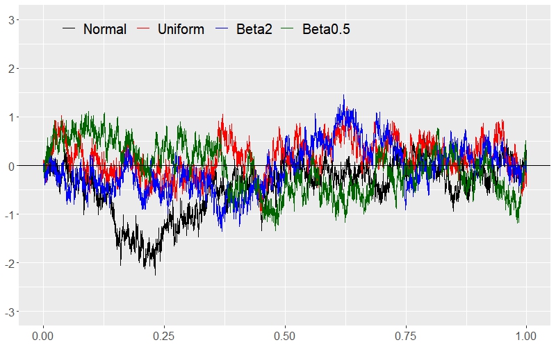
(a) Trajectories

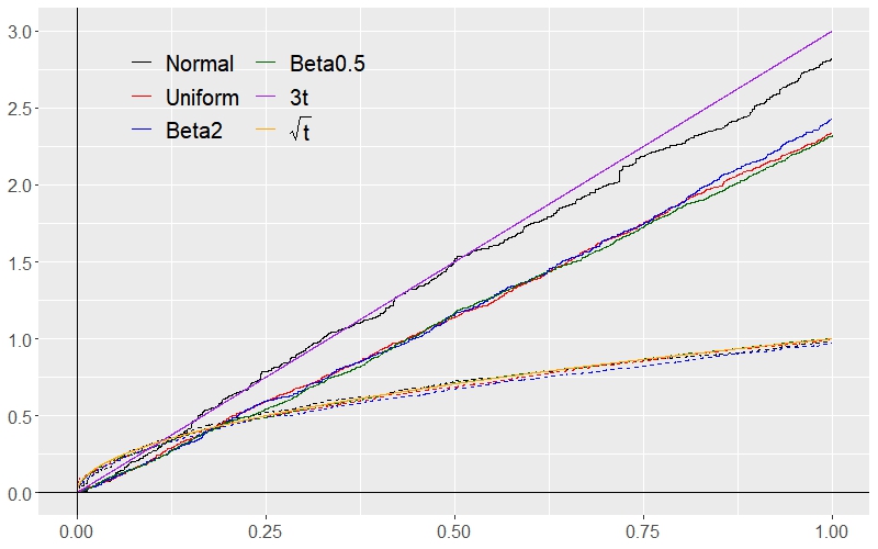
(b) Quartic and scaled quadratic variations

Figure 7: Fractional processes in (45) with $\displaystyle H=0.25$, truncated at level $\displaystyle n=12$

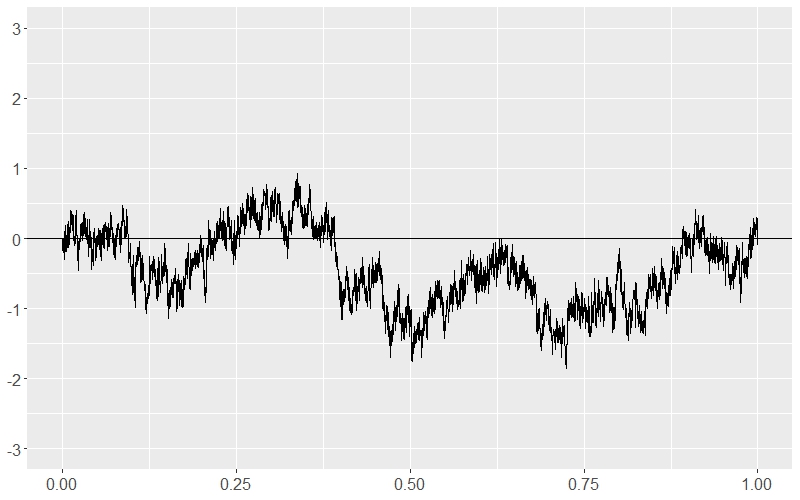
(a) A trajectory

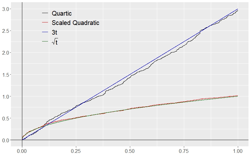
(b) Quartic and scaled quadratic variations

Figure 8: $\displaystyle Y^{H}_{mix}$ in (46) with $\displaystyle H=0.25$, truncated at level $\displaystyle n=12$

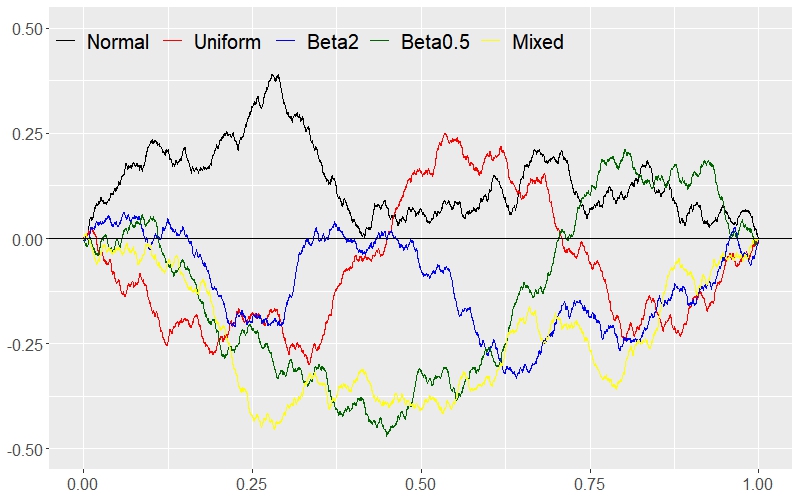
(a) Trajectories

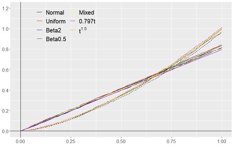
(b) $\displaystyle\frac{3}{4}$-th variation and scaled quadratic variations

Figure 9: Fractional processes in (45), (46) with $\displaystyle H=0.75$, truncated at level $\displaystyle n=12$

Remark 6.6 (Methods of simulation).

For simulating and plotting sample paths of Examples in Sections 5 and 6, we used the R language. Since the Schauder coefficients of the examples in Section 5 are independent, random sample generating functions in R are used when simulating the coefficients. For the examples in Section 6, as the Schauder coefficients are correlated, we first constructed a very large copula with the covariance structure given by (42), and randomly generated samples from the copula with different marginal distributions (uniform and beta). As this process requires a lot of computations, we only used the dyadic partition sequence and truncated up to level $\displaystyle n=12$ for simulating fake fBMs, whereas we truncated up to level $\displaystyle n=15$ and considered non-dyadic partition sequence (Example 6) for fake Brownian motions. We finally note that sample paths may be visually different when different truncation levels are used, especially for ‘rougher’ paths, as Figure 10 illustrates.

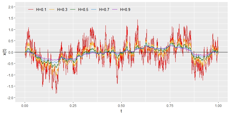
(a) n=10

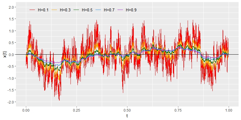
(b) n=12

Figure 10: Uniform independent Schauder coefficients for different Hurst indices $\displaystyle H$, truncated up to level $\displaystyle n=10$ and $\displaystyle n=12$, respectively.

6.3 Normality tests on the marginal distributions of fake fBMs

Even though the fake fBM in the previous subsection are non-Gaussian, here we do some normality tests for their marginal distributions as we did in Section 5.3. We also simulated $\displaystyle 5000$ sample paths of the fake process $\displaystyle Y^{H}_{mix}$ in Example 8, defined on $\displaystyle[0,1]$ along the dyadic partitions, truncated to the level $\displaystyle n=12$. We randomly chose $\displaystyle 10$ dyadic points $\displaystyle t_{i}\in(0,1)$ and took $\displaystyle 5000$ sample values $\displaystyle Y^{H}_{mix}(t_{i})$ at each $\displaystyle t_{i}$ for $\displaystyle i=1,\cdots,10$. Then, we did the same normality tests to find out whether those $\displaystyle 5000$ sample values for each point $\displaystyle t_{i}$ are drawn from a Gaussian distribution.

Table 2: $\displaystyle p$-values for the statistical tests for $\displaystyle Y_{mix}$ with Hurst index $\displaystyle H=0.25$ at $\displaystyle 10$ randomly chosen dyadic points, truncated at level $\displaystyle n=12$.

point $\displaystyle t_{i}$	Shapiro-Wilk	Kolmogorov-Smirnov	Jarque-Bera
1240/$\displaystyle 2^{12}$	0.1095	0.9568	0.1108
3824/$\displaystyle 2^{12}$	0.5994	0.6330	0.7276
381/$\displaystyle 2^{12}$	0.4229	0.6290	0.2309
361/$\displaystyle 2^{12}$	0.5681	0.8310	0.6793
1484/$\displaystyle 2^{12}$	0.0765	0.3724	0.0817
3881/$\displaystyle 2^{12}$	0.9323	0.9887	0.8707
3719/$\displaystyle 2^{12}$	0.5606	0.8071	0.3677
1618/$\displaystyle 2^{12}$	0.2488	0.9629	0.2385
3807/$\displaystyle 2^{12}$	0.4974	0.9755	0.3908
656/$\displaystyle 2^{12}$	0.3675	0.7949	0.3639

As we can observe from Table 2, all the $\displaystyle p$-values are bigger than $\displaystyle 5\%$, meaning we should not reject the null hypothesis (with a significance level of $\displaystyle 0.05$) stating that our sample values are drawn from a Gaussian distribution. Figure 11 also gives histograms and Q-Q plots of the $\displaystyle 5000$ sample values of $\displaystyle Y^{H}_{mix}(t)$ at another two (randomly chosen dyadic) points, $\displaystyle t=1240/2^{12}$ and $\displaystyle 3881/2^{12}$.

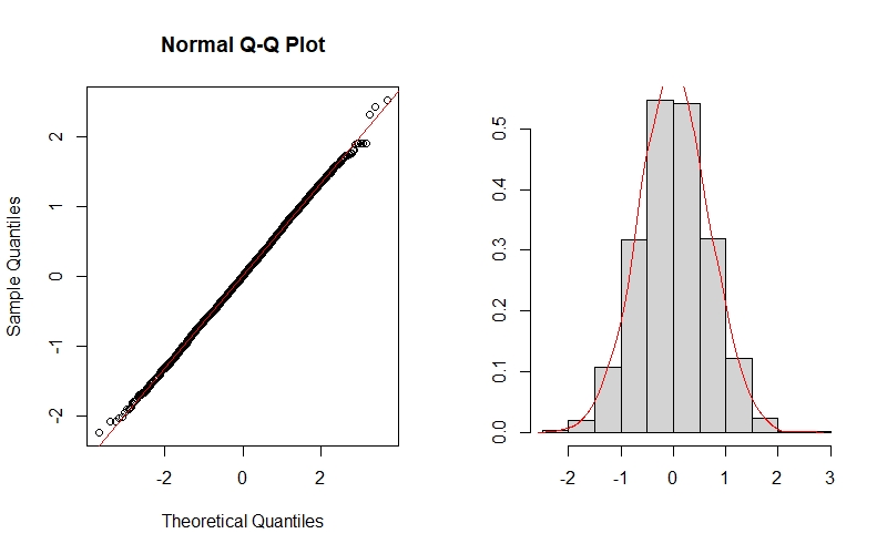
(a) level $\displaystyle n=12$, time $\displaystyle t=1240/2^{12}$

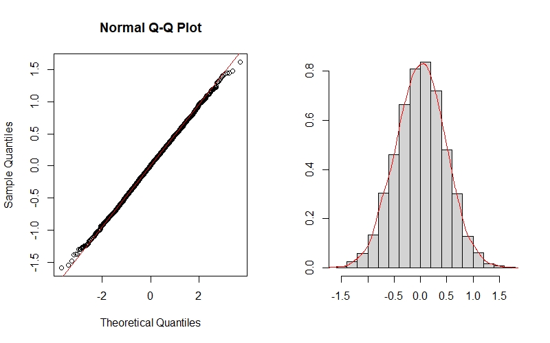
(b) level $\displaystyle n=12$, time $\displaystyle t=3881/2^{12}$

Figure 11: Q-Q plots and histograms for 5000 sample points of $\displaystyle Y^{H}_{mix}$ with $\displaystyle H=0.25$.

Despite the marginal distributions of the fake fBMs $\displaystyle Y^{H}_{mix}$ are not theoretically Gaussian, the simulation study concludes that commonly used statistical tests fail to identify the fake process as non-Gaussian.

7 Moments of Schauder coefficients

In the previous section, we only matched the first two moments of the Schauder coefficients of the fake processes with that of real fBMs such that the fake processes have the property (fBM ii), namely, the first two (joint) moments of finite-dimensional marginal distributions coincide with that of fBMs. The following result generalizes this to higher-order moments that the finite (joint) moments of the Schauder coefficients uniquely determine the finite (joint) moments of the marginal distribution of the process up to the same order.

Theorem 7.1 (Matching moments).

Consider the Schauder representations of two processes $\displaystyle X$ and $\displaystyle Y$, defined on $\displaystyle[0,T]$, along the same finitely refining partition sequence $\displaystyle\pi$:

$$X(t)=\sum_{m=0}^{\infty}\sum_{k\in I_{m}}\theta^{X}_{m,k}e^{\pi}_{m,k}(t),\qquad Y(t)=\sum_{m=0}^{\infty}\sum_{k\in I_{m}}\eta^{Y}_{m,k}e^{\pi}_{m,k}(t).$$

Suppose that the two families of random Schauder coefficients $\displaystyle\{\theta^{X}_{m,k}\}$ and $\displaystyle\{\eta^{Y}_{m,k}\}$ have the same finite moments up to order $\displaystyle\ell$ for some $\displaystyle\ell\in\mathbb{N}$, i.e., the identity

$$\mathbb{E}\left[\prod_{i=1}^{n}\theta^{X}_{m_{i},k_{i}}\right]=\mathbb{E}\left[\prod_{i=1}^{n}\eta^{Y}_{m_{i},k_{i}}\right]$$ (47)

holds for every $\displaystyle n\leq\ell$ and arbitrary $\displaystyle n$ pairs $\displaystyle(m_{i},k_{i})_{i=1}^{n}$ such that $\displaystyle m_{i}\in\mathbb{N}_{0}$, $\displaystyle k_{i}\in I_{m_{i}}$. If we have

$$\displaystyle\sum_{m_{1},k_{1}}\cdots\sum_{m_{\ell},k_{\ell}}\mathbb{E}\bigg{|}\prod_{j=1}^{\ell}\theta^{X}_{m_{j},k_{j}}\bigg{|}\bigg{(}\prod_{j=1}^{\ell}e^{\pi}_{m_{j},k_{j}}(t_{j})\bigg{)}<\infty,\quad\text{ and }$$ (48)

$$\displaystyle\sum_{m_{1},k_{1}}\cdots\sum_{m_{\ell},k_{\ell}}\mathbb{E}\bigg{|}\prod_{j=1}^{\ell}\eta^{Y}_{m_{j},k_{j}}\bigg{|}\bigg{(}\prod_{j=1}^{\ell}e^{\pi}_{m_{j},k_{j}}(t_{j})\bigg{)}<\infty,$$

for any $\displaystyle\ell$ pairs $\displaystyle(m_{i},k_{i})_{i=1}^{\ell}$ with $\displaystyle m_{i}\in\mathbb{N}_{0}$, $\displaystyle k_{i}\in I_{m_{i}}$ and $\displaystyle\ell$ points $\displaystyle t_{1},\cdots,t_{\ell}\in[0,T]$, then the finite-dimensional marginal distributions of $\displaystyle X$ and $\displaystyle Y$ have the same finite moments up to order $\displaystyle\ell$, that is,

$$\mathbb{E}\Big{[}\prod_{j=1}^{\ell}X(t_{j})\Big{]}=\mathbb{E}\Big{[}\prod_{j=1}^{\ell}Y(t_{j})\Big{]}.$$

In particular, if $\displaystyle\{\theta^{X}_{m,k}\}$ and $\displaystyle\{\eta^{Y}_{m,k}\}$ have the same finite moments and the inequalities in (48) hold for every order $\displaystyle\ell\in\mathbb{N}$, then the finite-dimensional marginal distributions of $\displaystyle X$ and $\displaystyle Y$ have the same finite moments for every order.

Proof.

First, the $\displaystyle\ell$-th order moment of the marginal distribution of $\displaystyle X$ at the points $\displaystyle 0\leq t_{1}\leq\cdots\leq t_{\ell}\leq T$ is well-defined due to Fatou’s lemma and (48):

$$\displaystyle\mathbb{E}\Big{|}\prod_{j=1}^{\ell}X(t_{j})\Big{|} \displaystyle=\mathbb{E}\bigg{|}\sum_{m_{1},k_{1}}\cdots\sum_{m_{\ell},k_{\ell}}\Big{(}\prod_{j=1}^{\ell}\theta^{X}_{m_{j},k_{j}}\Big{)}\Big{(}\prod_{j=1}^{\ell}e^{\pi}_{m_{j},k_{j}}(t_{j})\Big{)}\bigg{|}$$

$$\displaystyle\leq\sum_{m_{1},k_{1}}\cdots\sum_{m_{\ell},k_{\ell}}\mathbb{E}\bigg{|}\prod_{j=1}^{\ell}\theta^{X}_{m_{j},k_{j}}\bigg{|}\bigg{(}\prod_{j=1}^{\ell}e^{\pi}_{m_{j},k_{j}}(t_{j})\bigg{)}<\infty.$$

Thus, we can derive from the above inequality and dominated convergence theorem that

$$\displaystyle\mathbb{E}\Big{[}\prod_{j=1}^{\ell}X(t_{j})\Big{]} \displaystyle=\mathbb{E}\bigg{[}\sum_{m_{1},k_{1}}\cdots\sum_{m_{\ell},k_{\ell}}\Big{(}\prod_{j=1}^{\ell}\theta^{X}_{m_{j},k_{j}}\Big{)}\Big{(}\prod_{j=1}^{\ell}e^{\pi}_{m_{j},k_{j}}(t_{j})\Big{)}\bigg{]}$$

$$\displaystyle=\sum_{m_{1},k_{1}}\cdots\sum_{m_{\ell},k_{\ell}}\bigg{(}\mathbb{E}\Big{[}\prod_{j=1}^{\ell}\theta^{X}_{m_{j},k_{j}}\Big{]}\Big{(}\prod_{j=1}^{\ell}e^{\pi}_{m_{j},k_{j}}(t_{j})\Big{)}\bigg{)}.$$

Since the last term $\displaystyle\prod_{j=1}^{\ell}e^{\pi}_{m_{j},k_{j}}(t_{j})$ is independent of the process $\displaystyle X$ and the $\displaystyle\ell$-th order moment of the coefficients $\displaystyle\{\theta^{X}_{m_{j},k_{j}}\}_{j=1}^{\ell}$ can be replaced by that of $\displaystyle\{\eta^{Y}_{m_{j},k_{j}}\}_{j=1}^{\ell}$, we can proceed backwards to show that the right-hand side is equal to $\displaystyle\mathbb{E}\Big{[}\prod_{j=1}^{\ell}Y(t_{j})\Big{]}$. ∎

Next, we show that the (real) fractional Brownian process $\displaystyle B^{H}(t)-Zt$ of (36) satisfies the condition (48) in Theorem 7.1.

Proposition 7.2.

For the Schauder representation (36) of fBM $\displaystyle B^{H}$ along a balanced and complete refining partition sequence $\displaystyle\pi$, we have

$$\sum_{m_{1},k_{1}}\cdots\sum_{m_{\ell},k_{\ell}}\mathbb{E}\bigg{|}\prod_{j=1}^{\ell}\theta^{B^{H}}_{m_{j},k_{j}}\bigg{|}\bigg{(}\prod_{j=1}^{\ell}e^{\pi}_{m_{j},k_{j}}(t_{j})\bigg{)}<\infty$$ (49)

for all $\displaystyle\ell$ pairs $\displaystyle(m_{i},k_{i})_{i=1}^{\ell}$ with $\displaystyle m_{i}\in\mathbb{N}_{0}$, $\displaystyle k_{i}\in I_{m_{i}}$ and $\displaystyle\ell$ points $\displaystyle t_{1},\cdots,t_{\ell}\in[0,T]$ for every $\displaystyle\ell\in\mathbb{N}$.

Proof.

Since each coefficient $\displaystyle\theta^{B^{H}}_{m_{j},k_{j}}$ is distributed as $\displaystyle\sigma_{m_{j},k_{j}}N(0,1)$, a generalized Hölder inequality gives

$$\displaystyle\mathbb{E}\bigg{|}\prod_{j=1}^{\ell}\theta^{B^{H}}_{m_{j},k_{j}}\bigg{|}\leq\prod_{j=1}^{\ell}\Big{(}\mathbb{E}\big{|}\theta^{B^{H}}_{m_{j},k_{j}}\big{|}^{\ell}\Big{)}^{\frac{1}{\ell}}=\prod_{j=1}^{\ell}\Big{(}\sigma_{m_{j},k_{j}}(C_{\ell})^{\frac{1}{\ell}}\Big{)}=C_{\ell}\prod_{j=1}^{\ell}\sigma_{m_{j},k_{j}},$$

where we denote $\displaystyle C_{\ell}:=\mathbb{E}|N(0,1)|^{\ell}<\infty$ the $\displaystyle\ell$-th moment of the standard half-normal distribution. Now that $\displaystyle\pi$ is balanced and complete refining, we have the bound $\displaystyle\sigma_{m_{j},k_{j}}\leq K|\pi^{m_{j}+1}|^{\frac{2H-1}{2}}$ for some positive constant $\displaystyle K>0$, from the expression (37). We finally recall the bound (9) to derive

$$\displaystyle\sum_{m_{1},k_{1}}\cdots\sum_{m_{\ell},k_{\ell}} \displaystyle\mathbb{E}\bigg{|}\prod_{j=1}^{\ell}\theta^{B^{H}}_{m_{j},k_{j}}\bigg{|}\bigg{(}\prod_{j=1}^{\ell}e^{\pi}_{m_{j},k_{j}}(t_{j})\bigg{)}\leq C_{\ell}\sum_{m_{1},k_{1}}\cdots\sum_{m_{\ell},k_{\ell}}\bigg{(}\prod_{j=1}^{\ell}\sigma_{m_{j},k_{j}}e^{\pi}_{m_{j},k_{j}}(t_{j})\bigg{)}$$

$$\displaystyle=C_{\ell}\prod_{j=1}^{\ell}\bigg{(}\sum_{m_{j},k_{j}}\sigma_{m_{j},k_{j}}e^{\pi}_{m_{j},k_{j}}(t_{j})\bigg{)}\leq C_{\ell}\prod_{j=1}^{\ell}\bigg{(}\sum_{m_{j}}KM|\pi^{m_{j}+1}|^{\frac{2H-1}{2}}|\pi^{m_{j}+1}|^{\frac{1}{2}}\bigg{)}$$

$$\displaystyle=C_{\ell}KM\prod_{j=1}^{\ell}\bigg{(}\sum_{m_{j}}|\pi^{m_{j}+1}|^{H}\bigg{)}<\infty.$$

∎

The generic form of the Schauder coefficients of the fake fractional processes in Examples 7 and 8 are distributed as $\displaystyle\Sigma_{m,k}R_{m,k}$, where each $\displaystyle R_{m,k}$ is a random variable with compact support, thus has finite moments of all orders. Therefore, the same argument in the proof of Proposition 7.2 can be applied to show the same finiteness condition (49) for the fake processes. Theorem 7.1 then concludes that if we match the joint moments of the Schauder coefficients up to more high-order (than the second order which we did in the previous subsections) with that of the Schauder coefficients of fBM, then the finite-dimensional marginal distribution of the fake process should have the same finite joint moments as fBMs up to the same high-order.

Jarque-Bera test actually measures how the third and fourth moments of given samples are close to those moments of normal distributions. If we match the moments of the Schauder coefficients up to the fourth order as real fBMs, then the first four moments of marginal distributions of the fake process will theoretically coincide with those of real fBMs (see Remark 5.4).

Proposition 7.2 immediately yields the following convergence result.

Corollary 7.3.

Along a balanced and complete refining partition sequence $\displaystyle\pi$ of $\displaystyle[0,1]$, let us recall the covariances in (38) and (6.1) between the Schauder coefficients of fBM. The following identity always holds for any $\displaystyle s,t\in[0,T]$:

$$\sum_{m=-1}^{n}\sum_{k\in I_{m}}\sum_{m^{\prime}=-1}^{n}\sum_{k^{\prime}\in I_{m^{\prime}}}\sigma_{m,k,m^{\prime},k^{\prime}}e^{\pi}_{m,k}(t)e^{\pi}_{m^{\prime},k^{\prime}}(s)\xlongrightarrow{n\rightarrow\infty}\frac{1}{2}(|t|^{2H}+|s|^{2H}-|t-s|^{2H}).$$ (50)

Proof.

From Proposition 2.9 and the representation (36) with notation

$$B_{n}^{H}(t):=\sum_{m=-1}^{n}\sum_{k\in I_{m}}\theta_{m,k}^{B^{H}}e^{\pi}_{m,k}(t),$$

we have the convergence for any $\displaystyle t\in[0,1]$

$$B_{n}^{H}(t)\xrightarrow{n\rightarrow\infty}B^{H}(t)\quad\mathbb{P}-a.e.$$

Then, we also have the following convergence

$$\mathbb{E}\big{[}B^{H}_{n}(t)B^{H}_{n}(s)\big{]}\xlongrightarrow{n\to\infty}\mathbb{E}\big{[}B^{H}(t)B^{H}(s)\big{]}=\frac{1}{2}(|t|^{2H}+|s|^{2H}-|t-s|^{2H}),$$

from the bound (49) and the Dominated convergence theorem. The left-hand side is just equal to that of (50). ∎

Note that the Schauder functions $\displaystyle e^{\pi}_{m,k}$ and the quantities $\displaystyle\sigma_{m,k,m^{\prime},k^{\prime}}$ of Corollary 7.3 are completely deterministic and depend only on the choice of the partition sequence $\displaystyle\pi$ but not on paths of fBM $\displaystyle B^{H}$.

We conclude this section with the following corollary of Theorem 7.1; matching the moments of the Schauder coefficients up to a higher order gives rise to an additional property of the fake fractional processes of $\displaystyle Y^{H}$ in Theorem 6.2.

Corollary 7.4.

Besides conditions (a) and (b) of Theorem 6.2, suppose that the following condition also holds

1. the reciprocal $\displaystyle 1/H$ of Hurst index is an even integer, which we denote by $\displaystyle p:=1/H\in 2\mathbb{N}$, and the two families of Schauder coefficients $\displaystyle\{\theta^{Y^{H}}_{m,k}\}$ and $\displaystyle\{\theta^{B^{H}}_{m,k}\}$ satisfy the conditions (47) and (48) up to order $\displaystyle\ell=p$, such that the marginal distributions have the same moments up to order $\displaystyle p$, i.e.,

   $$\mathbb{E}\Big{[}\prod_{j=1}^{n}Y^{H}(t_{j})\Big{]}=\mathbb{E}\Big{[}\prod_{j=1}^{n}B^{H}(t_{j})\Big{]}$$ (51)

   holds for every $\displaystyle n\leq p$.

Then, the fake fractional process $\displaystyle Y^{H}$ shares an additional property (fBM vii) with fBM $\displaystyle B^{H}$:

1. we have the convergence of the (discrete) $\displaystyle p$-th variation for every $\displaystyle t\in[0,1]$

   $$\lim_{n\rightarrow\infty}\mathbb{E}\bigg{[}\sum_{\begin{subarray}{c}t^{n}_{i},t^{n}_{i+1}\in\pi^{n}\\ t^{n}_{i+1}\leq t\end{subarray}}\big{|}Y^{H}(t^{n}_{i+1})-Y^{H}(t^{n}_{i})\big{|}^{p}\bigg{]}=C_{p}t,$$ (52)

   where we denote $\displaystyle C_{p}:=\mathbb{E}|N(0,1)|^{p}$.

Proof.

Note that conditions (a) and (c) are the same if $\displaystyle p=2$. Expanding the $\displaystyle p$-th power with the Binomial theorem and equating each moment as in (51), we have

$$\mathbb{E}\big{|}Y^{H}(t^{n}_{i+1})-Y^{H}(t^{n}_{i})\big{|}^{p}=\mathbb{E}\big{|}B^{H}(t^{n}_{i+1})-B^{H}(t^{n}_{i})\big{|}^{p}.$$

From the stationary increments property and self-similarity of fBM, we further derive

$$\mathbb{E}\big{|}B^{H}(t^{n}_{i+1})-B^{H}(t^{n}_{i})\big{|}^{p}=\mathbb{E}\big{|}B^{H}(t^{n}_{i+1}-t^{n}_{i})\big{|}^{p}=|t^{n}_{i+1}-t^{n}_{i}|^{pH}\mathbb{E}\big{|}B^{H}(1)\big{|}^{p}=C_{p}|t^{n}_{i+1}-t^{n}_{i}|.$$

Denoting

$$[Y^{H}]^{(p)}_{\pi_{n}}(t):=\sum_{\begin{subarray}{c}t^{n}_{i},t^{n}_{i+1}\in\pi^{n}\\ t^{n}_{i+1}\leq t\end{subarray}}\big{|}Y^{H}(t^{n}_{i+1})-Y^{H}(t^{n}_{i})\big{|}^{p},$$

we have

$$\displaystyle\mathbb{E}\big{[}[Y^{H}]^{(p)}_{\pi_{n}}(t)\big{]} \displaystyle=\sum_{\begin{subarray}{c}t^{n}_{i},t^{n}_{i+1}\in\pi^{n}\\ t^{n}_{i+1}\leq t\end{subarray}}\mathbb{E}\big{|}Y^{H}(t^{n}_{i+1})-Y^{H}(t^{n}_{i})\big{|}^{p}$$

$$\displaystyle=\sum_{\begin{subarray}{c}t^{n}_{i},t^{n}_{i+1}\in\pi^{n}\\ t^{n}_{i+1}\leq t\end{subarray}}\mathbb{E}\big{|}B^{H}(t^{n}_{i+1})-B^{H}(t^{n}_{i})\big{|}^{p}=C_{p}\sum_{\begin{subarray}{c}t^{n}_{i},t^{n}_{i+1}\in\pi^{n}\\ t^{n}_{i+1}\leq t\end{subarray}}|t^{n}_{i+1}-t^{n}_{i}|,$$

and the last term converges to $\displaystyle C_{p}t$ as $\displaystyle n\rightarrow\infty$. ∎

In Figures 7 and 8 (b), the graphs of the quartic variations of fake processes seem to be linear, even though we didn’t match the Schauder coefficients up to order $\displaystyle p=1/H=4$. Especially, the quartic variation of $\displaystyle Y^{H}_{mix}$ in Figure 8 (b) has almost the same slope as that of real fBM.

Furthermore, the graphs of the $\displaystyle 3/4$-th variations in Figure 9 (b) also look linear, though the Hurst index $\displaystyle H=3/4$ is not a reciprocal of an even integer. Therefore, we conjecture that the $\displaystyle(1/H)$-th variation of fake fractional processes along a balanced, completely refining partition sequence $\displaystyle\pi$ will be linear with slope equal to $\displaystyle C_{1/H}:=\mathbb{E}[|N(0,1)|^{\frac{1}{H}}]$, if we match the first $\displaystyle m=\Big{\lceil}\frac{1}{H}\Big{\rceil}$ moments of the Schauder coefficients with that of real fBM with Hurst index $\displaystyle H$.

8 Proofs of Theorems 5.1 and 6.2

Proof of Theorem 5.1.

We shall prove each property from (BM i) to (BM vii) one by one.

(BM i) Since condition (b) coincides with that of Lemma 2.10 with $\displaystyle\epsilon=1/2$, the result follows from Lemma 2.10.

(BM ii) First, Proposition 7.2 for the case $\displaystyle H=1/2$ shows that the family of coefficients $\displaystyle(\theta^{B}_{m,k})$ satisfies the condition (48) for $\displaystyle\ell=2$. Moreover, we have the uniform bound

$$\mathbb{E}\big{|}\theta^{Y}_{m_{1},k_{1}}\theta^{Y}_{m_{2},k_{2}}\big{|}\leq\frac{1}{2}\Big{(}\mathbb{E}[(\theta^{Y}_{m,k})^{2}]+\mathbb{E}[(\theta^{Y}_{m^{\prime},k^{\prime}})^{2}]\Big{)}=\mathbb{E}[(\theta^{Y}_{m,k})^{2}]\leq\sqrt{\mathbb{E}[(\theta^{Y}_{m,k})^{4}]}<\infty,$$

and the argument in the proof of Proposition 7.2 yields that the condition (48) for $\displaystyle\ell=2$ is satisfied for the family $\displaystyle(\theta^{Y}_{m,k})$ as well. Theorem 7.1 then proves the property, since we matched the mean and covariance of the Schauder coefficients, i.e., $\displaystyle\mathbb{E}[\theta^{Y}_{m,k}]=\mathbb{E}[\theta^{B}_{m,k}]=0$, $\displaystyle\mathbb{E}[\theta^{Y}_{m,k}\theta^{Y}_{m^{\prime},k^{\prime}}]=\mathbb{E}[\theta^{B}_{m,k}\theta^{B}_{m^{\prime},k^{\prime}}]=\mathbbm{1}_{m=m^{\prime}}\mathbbm{1}_{k=k^{\prime}}$.

(BM iii) From (BM ii), we have

$$\displaystyle\mathbb{E}[(Y(t)-Y(s))(Y(v)-Y(u))] \displaystyle=\mathbb{E}[Y(t)Y(v)]-\mathbb{E}[Y(t)Y(u)]-\mathbb{E}[Y(s)Y(v)]+\mathbb{E}[Y(s)Y(u)]$$

$$\displaystyle=t-t-s+s=0.$$

We note that Brownian motion has independent increments, however, uncorrelatedness between increments does not generally imply independent increments for non-Gaussian process $\displaystyle Y$.

(BM iv) This follows from Corollary 3.6.

(BM iv’) of Remark 5.2 The quantity $\displaystyle\sup_{m,k}(|\theta^{Y}_{m,k}||\pi^{m+1}|^{\frac{1}{2}-\alpha})$ is finite if and only if $\displaystyle\alpha\leq 1/2$, thus Theorem 3.4 yields the result.

(BM v) This is obvious from the construction of $\displaystyle Y$.

(BM vi) The process $\displaystyle Y$ belongs to the class $\displaystyle\mathcal{B}^{\pi}$ in (13) of [8], thus $\displaystyle[Y]^{(2)}_{\pi}(t)=t$ almost surely from Theorem 5.2 of [8].

(BM vii) The process $\displaystyle Y$ further belongs to the class $\displaystyle\mathcal{A}^{\pi}$ in (31) of [8], thus Theorem 6.5 of [8] proves the property. ∎

Proof of Theorem 6.2.

(fBM i) Note that condition (b) is from condition (ii) of Lemma 2.10, for $\displaystyle\epsilon=H$, thus $\displaystyle Y^{H}$ has a continuous path almost surely.

(fBM ii) Proposition 7.2 proves that the family of coefficients $\displaystyle(\theta^{B}_{m,k})$ (of real fBM) satisfies the condition (48) for $\displaystyle\ell=2$. Furthermore, Cauchy-Schwarz inequality and condition (a) deduce

$$\mathbb{E}\big{|}\theta^{Y^{H}}_{m_{1},k_{1}}\theta^{Y^{H}}_{m_{2},k_{2}}\big{|}\leq\sqrt{\mathbb{E}[(\theta^{Y^{H}}_{m,k})^{2}]\mathbb{E}[(\theta^{Y^{H}}_{m^{\prime},k^{\prime}})^{2}]}=\sigma_{m,k}\sigma_{m^{\prime},k^{\prime}},$$

and the argument in the proof of Proposition 7.2 yields that the condition (48) for $\displaystyle\ell=2$ is satisfied for the family $\displaystyle(\theta^{Y^{H}}_{m,k})$ as well. Theorem 7.1 now proves the property, since we matched the mean and covariance of the two families of Schauder coefficients $\displaystyle(\theta^{B^{H}}_{m,k})$ and $\displaystyle(\theta^{Y^{H}}_{m,k})$ in condition (a).

(fBM iii) This is again straightforward from (fBM ii).

(fBM iv) This follows from Corollary 3.6.

(fBM iv’) of Remark 6.3 We have the bounds

$$\sup_{m,k}\big{(}|\theta^{Y^{H}}_{m,k}||\pi^{m+1}|^{\frac{1}{2}-\alpha}\big{)}\leq C\sup_{m}\big{(}|\pi^{m+1}|^{H-\frac{1}{2}}|\pi^{m+1}|^{\frac{1}{2}-\alpha}\big{)}=C\sup_{m}|\pi^{m+1}|^{H-\alpha},$$

where the last term is finite if and only if $\displaystyle\alpha\leq H$, therefore Theorem 3.4 proves (fBM iv’).

(fBM v) This is obvious from the construction of $\displaystyle Y^{H}$.

(fBM vi) From (fBM ii), the first two moments of the marginal distribution of $\displaystyle Y^{H}$ coincide with that of fBM $\displaystyle B^{H}$. Thus, we have

$$\mathbb{E}\big{|}Y^{H}(t^{n}_{i+1})-Y^{H}(t^{n}_{i})\big{|}^{2}=\mathbb{E}\big{|}B^{H}(t^{n}_{i+1})-B^{H}(t^{n}_{i})\big{|}^{2}=|t^{n}_{i+1}-t^{n}_{i}|^{2H}=|\pi^{n}|^{2H},$$

for any consecutive partition points $\displaystyle t^{n}_{i},t^{n}_{i+1}\in\pi^{n}$. The expectation on the left-hand side of (44) is now equal to

$$\Big{\lfloor}\frac{|\pi^{n}|}{t}\Big{\rfloor}^{1-2H}\sum_{\begin{subarray}{c}t^{n}_{i},t^{n}_{i+1}\in\pi^{n}\\ t^{n}_{i+1}\leq t\end{subarray}}|\pi^{n}|^{2H}=\Big{\lfloor}\frac{|\pi^{n}|}{t}\Big{\rfloor}^{1-2H}\times|\pi^{n}|^{2H}\times\Big{\lfloor}\frac{t}{|\pi^{n}|}\Big{\rfloor},$$

and the last expression converges to $\displaystyle t^{2H}$ as $\displaystyle n\to\infty$. ∎

9 Conclusion

Using (generalized) Schauder representation, we constructed a stochastic process with any given Hölder regularity by controlling the growth of Schauder coefficients along a given partition sequence on a finite interval (Theorem 3.4). Moreover, we can make the finite moments of the marginal distribution of the process as we want, by controlling the joint moments between the Schauder coefficients (Theorem 7.1). These results are combined to suggest a new way of constructing stochastic processes which are statistically indistinguishable from Brownian motion or fractional Brownian motions.

Our results bring two important messages for mathematical modeling with stochastic processes, especially in finance. First, when measuring the roughness of a given function or process (e.g. for stock volatility), Hölder regularity and variation index are two different notions. Therefore, when observing a sample path from a process, we should not measure its Hölder roughness by computing $\displaystyle p$-th variation. Secondly, Brownian motion and fractional Brownian motions have been widely used for modeling stochastic phenomena in various fields, due to their full-fledged theory. However, our construction of fake Brownian motions and fake fractional Brownian motions suggests that a ‘model-free’ approach is important; we cannot conclude from a given dataset that the underlying process follows certain dynamics involving either Brownian motion or fractional Brownian motion, even though it exhibits the same pathwise and statistical properties as those Gaussian processes.

Our method of construction in Sections 5 and 6 can be also useful for generating very diverse sets of training data for (deep) neural networks modeling financial time series (e.g. [18]), which we leave as future work.

References

- [1] J. Albin, A continuous non-brownian motion martingale with brownian motion marginal distributions, Statistics & probability letters, 78 (2008), pp. 682–686.
- [2] E. Bayraktar, H. V. Poor, and K. R. Sircar, Estimating the fractal dimension of the S&P 500 index using wavelet analysis, International Journal of Theoretical and Applied Finance, 7 (2004), pp. 615–643.
- [3] M. Beiglböck, G. Lowther, G. Pammer, and W. Schachermayer, Faking Brownian motion with continuous Markov martingales, arXiv, (2021).
- [4] F. Biagini, Y. Hu, B. Øksendal, and T. Zhang, Stochastic Calculus for Fractional Brownian Motion and Applications, Springer-Verlag London, 01 2008.
- [5] Z. Ciesielski, On the isomorphisms of the spaces and , Bull. Acad. Polon. Sci. Sér. Sci. Math. Astronom. Phys., 8 (1960), pp. 217–222.
- [6] J. Collins and C. De Luca, Upright, correlated random walks: A statistical-biomechanics approach to the human postural control system, Chaos: An Interdisciplinary Journal of Nonlinear Science, 5 (1995), pp. 57–63.
- [7] R. Cont and P. Das, Measuring the roughness of a signal, Working Paper, (2022).
- [8] , Quadratic variation along refining partitions: Constructions and examples, Journal of Mathematical Analysis and Applications, 512 (2022), p. 126173.
- [9] , Quadratic variation and quadratic roughness, Bernoulli, 29 (2023), pp. 496 – 522.
- [10] R. Cont and N. Perkowski, Pathwise integration and change of variable formulas for continuous paths with arbitrary regularity, Transactions of the American Mathematical Society, 6 (2019), pp. 134–138.
- [11] K. Daoudi, J. Lévy Véhel, and Y. Meyer, Construction of continuous functions with prescribed local regularity, Constructive Approximation, 14 (1998), pp. 349–385.
- [12] A. Echelard, 2-microlocal analysis and application to noise reduction, theses, Ecole Centrale de Nantes (ECN); University of Nantes, Nov. 2007.
- [13] D. V. Filatova and M. Grzywaczewski, Mathematical modeling in selected biological systems with fractional brownian motion, in 2008 Conference on Human System Interactions, IEEE, 2008, pp. 909–914.
- [14] H. Föllmer, Calcul d’Itô sans probabilités, in Seminar on Probability, XV (Univ. Strasbourg, Strasbourg, 1979/1980) (French), vol. 850 of Lecture Notes in Math., Springer, Berlin, 1981, pp. 143–150.
- [15] N. Gantert, Self-similarity of Brownian motion and a large deviation principle for random fields on a binary tree, Prob. Th. Rel. Fields, 98 (1994), pp. 7–20.
- [16] S. Gurbatov, S. Simdyankin, E. Aurell, U. Frisch, and G. Toth, On the decay of burgers turbulence, Journal of Fluid Mechanics, 344 (1997), pp. 339–374.
- [17] A. Haar, Zur Theorie der orthogonalen Funktionen systeme, Mathematische Annalen, 69 (1910), pp. 331–371.
- [18] M. Hamdouche, P. Henry-Labordere, and H. Pham, Generative modeling for time series via schrödinger bridge, 2023. Preprint, arXiv:2304.05093.
- [19] K. Hamza and F. C. Klebaner, A family of non-gaussian martingales with gaussian marginals, Journal of Applied Mathematics and Stochastic Analysis, 2007 (2007).
- [20] X. Han and A. Schied, The Hurst roughness exponent and its model-free estimation, arXiv, (2021).
- [21] D. Hobson, Mimicking martingales, The Annals of Applied Probability, 26 (2016), pp. 2273 – 2303.
- [22] D. G. Hobson, Fake exponential Brownian motion, Statistics & Probability Letters, 83 (2013), pp. 2386–2390.
- [23] S. Jaffard, Wavelet techniques in multifractal analysis, in Fractal geometry and applications: a jubilee of Benoît Mandelbrot, Part 2, vol. 72 of Proc. Sympos. Pure Math., Amer. Math. Soc., Providence, RI, 2004, pp. 91–151.
- [24] I. Karatzas and S. E. Shreve, Brownian Motion and Stochastic Calculus, vol. 113 of Graduate Texts in Mathematics, Springer-Verlag, New York, second ed., 1991.
- [25] W. E. Leland, M. S. Taqqu, W. Willinger, and D. V. Wilson, On the self-similar nature of ethernet traffic (extended version), IEEE/ACM Transactions on networking, 2 (1994), pp. 1–15.
- [26] A. W. Lo, Long-term memory in stock market prices, Econometrica: Journal of the Econometric Society, (1991), pp. 1279–1313.
- [27] D. B. Madan and M. Yor, Making markov martingales meet marginals: with explicit constructions, Bernoulli, (2002), pp. 509–536.
- [28] Y. Mishura, Stochastic Calculus for Fractional Brownian Motion and Related Processes, Lecture Notes in Mathematics, Springer Berlin, Heidelberg, first ed., 2008.
- [29] Y. Mishura and A. Schied, Constructing functions with prescribed pathwise quadratic variation, Journal of Mathematical Analysis and Applications, 482 (2016), pp. 117–1337.
- [30] Y. Mishura and E. Valkeila, An extension of the Lévy characterization to fractional Brownian motion, The Annals of Probability, 39 (2011), pp. 439 – 470.
- [31] K. Oleszkiewicz, On fake Brownian motions, Statistics & probability letters, 78 (2008), pp. 1251–1254.
- [32] L. C. G. Rogers, Arbitrage with Fractional Brownian motion, Mathematical Finance, 7 (1997), pp. 95–105.
- [33] T. Sadhu and K. J. Wiese, Functionals of fractional brownian motion and the three arcsine laws, Physical Review E, 104 (2021), p. 054112.
- [34] J. Schauder, Eine Eigenschaft des Haarschen Orthogonalsystems, Math. Z., 28 (1928), pp. 317–320.
- [35] A. Schied, On a class of generalized Takagi functions with linear pathwise quadratic variation, J. Math. Anal. Appl., 433 (2016), pp. 974–990.
- [36] Z. Semadeni, Schauder bases in Banach spaces of continuous functions, vol. 918 of Lecture Notes in Mathematics, Springer-Verlag, Berlin-New York, 1982.
- [37] M. S. Taqqu, V. Teverovsky, and W. Willinger, Is network traffic self-similar or multifractal?, Fractals, 5 (1997), pp. 63–73.