NLO + parton-shower generator for $\boldsymbol{Wc}$ production in the POWHEG BOX RES

Abstract

We present the implementation of a next-to-leading-order plus parton-shower event generator for the hadronic production of a heavy charm quark accompanied by a leptonically-decaying $W$ boson in the POWHEG BOX RES framework. We consider both signatures, i.e. $pp\to c\,\ell^{-}\bar{\nu}_{\ell}$ and $pp\to\bar{c}\,\ell^{+}{\nu}_{\ell}$, and we include exactly off-shell and spin-correlation effects, as well as off-diagonal Cabibbo-Kobayashi-Maskawa contributions. We present particle-level results, obtained interfacing our code with the Herwig7.2 and Pythia8.3 shower Monte Carlo event generators, including hadronization and underlying-event effects, and compare them against the data collected by the CMS Collaboration at $\sqrt{s}=13$ TeV.

1 Introduction

The production of a $W$ boson in association with a charm quark ($c$), tagged by the full reconstruction of the charmed $D$ hadron from the clear experimental signature of its decay products, is one of the main probe of the strange-quark content of the colliding particles at an hadron collider, such as the LHC. In fact, the leading contribution to $Wc$ production ($W^{-}c$ and $W^{+}\bar{c}$) comes from the scattering of a strange quark ($s$ or $\bar{s}$) and a gluon, from the two incoming hadrons, since the corresponding Cabibbo-Kobayashi-Maskawa (CKM) matrix element is the dominant one for this channel. The two leading-order (LO) Feynman diagrams for $Wc$ production are depicted in Fig. 1.

As first illustrated in Ref. Baur:1993zd , this process can be used to put constraints on the strange-quark content of the colliding hadrons, i.e. protons at the Large Hadron Collider (LHC). Several measurements of $Wc$ production have already been performed at the LHC as it went through the increasing energy upgrade from 7 to 13 TeV, by the ATLAS ATLAS:2014jkm ; ATLAS:2023ibp , the CMS CMS:2013wql ; CMS:2021oxn ; CMS:2018dxg and the LHCb Collaborations LHCb:2015bwt .

The next-to-leading order (NLO) QCD cross section for $Wc$ production has been known for a while, and studied both at the Tevatron Giele:1995kr and at the LHC Stirling:2012vh . More recently, the complete set of next-to-next-to-leading order (NNLO) QCD corrections to the dominant CKM-diagonal contribution have been computed in Ref. Czakon:2020coa and further extended with full CKM dependence, including the dominant NLO electro-weak corrections, in Ref. Czakon:2022khx , in the massless-charm limit.

The first dedicated NLO QCD + parton shower (PS) generator for $Wc$ production was done in Ref. Bevilacqua:2021ovq , within the PowHel event generator, based on the POWHEG method Nason:2004rx , with the $W$ boson decaying leptonically, including charm-quark mass effects in the hard-scattering matrix elements and a non-diagonal CKM matrix.

In this paper we describe the implementation of a NLO + parton-shower generator for the hadro-production of a massive charm quark accompanied by a leptonically-decaying $W$ boson in the POWHEG BOX RES framework Frixione:2007vw ; Alioli:2010xd ; Jezo:2015aia . We include exactly off-shell and spin-correlation effects, as well as off-diagonal CKM contributions.

The POWHEG BOX RES framework is able to deal with radiation off resonances. Although for the case at hand of QCD corrections to a leptonically decaying $W$ boson, the machinery of radiation off resonances is not necessary, since no QCD radiation can be emitted from the leptons, we have implemented $Wc$ production in this framework for several reasons:

1. Better handling of final-state radiation from heavy quarks, as radiation collinear to heavy partons is dealt with an appropriate importance sampling.

2. The future inclusion of NLO electro-weak corrections is facilitated, since the process is already in the right framework to deal with photon radiation, not only from quarks, but also from the charged lepton in the $W$ decay, where the virtuality of the resonance has to be preserved during the generation of the hardest radiation performed by the POWHEG BOX RES.

3. All the processes for which the NNLO+PS accuracy has been reached Mazzitelli:2020jio ; Mazzitelli:2021mmm ; Zanoli:2021iyp ; Gavardi:2022ixt using the MiNNLO_PS formalism Monni:2019whf ; Monni:2020nks are implemented in the POWHEG BOX RES framework. It would then be easier to implement also the NNLO QCD corrections to $Wc$ production in this framework too.

The paper is organized as follows. In Sect. 2 we give some technical details about the process we are studying at LO and NLO, we describe the change of scheme of our calculation and the default choice of the renormalization and factorization scales that we have used. In addition we give the numerical value of the input parameters we have used in our simulation, and we present the validation of the fixed-order NLO results. In Sect. 3 we give details of the matching of the NLO amplitudes with the POWHEG method, as implemented in the POWHEG BOX RES framework. We discuss the effects of the extra degrees of freedom offered by this matching and their numerical impact. In Sect. 4 we present a few interesting kinematic distributions computed with events obtained by completing the first radiation emission performed by the POWHEG BOX RES code, with three showering models, implemented in Herwig7.2 and Pythia8.3, and we discuss the differences. We also present results with full hadronization in place and in the presence of underlying events, and we compare them with the experimental data collected by the CMS Collaboration at 13 TeV.

The POWHEG BOX RES framework, together with the Wc generator, can be downloaded at http://powhegbox.mib.infn.it.

2 Contributing processes and technical details

In this section we discuss the implementation of the processes $pp\to\ell^{-}\bar{\nu}_{\ell}c$ and $pp\to\ell^{+}\nu_{\ell}\bar{c}$ at NLO QCD accuracy.

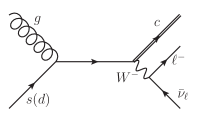
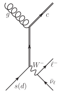
(a)

(b)

Figure 1: Feynman diagrams contributing to the partonic process $g\,s(d)\rightarrow\ell^{-}\,\bar{\nu}_{\ell}\,c$ at LO, in the $s$ channel (a), on the left, and $t$ channel (b), on the right. The heavy charm quark is represented as a double line.

We consider the $c$ quark to be massive, with all the other lighter quarks and anti-quarks treated as massless. At LO, the partonic subprocesses that contribute to $Wc$ production are

$${\displaystyle\begin{array}[]{l}g\,d\rightarrow\ell^{-}\,\bar{\nu}_{\ell}\,c\\ g\,s\rightarrow\ell^{-}\,\bar{\nu}_{\ell}\,c\\ g\,\bar{d}\rightarrow\ell^{+}\,\nu_{\ell}\,\bar{c}\\ g\,\bar{s}\rightarrow\ell^{+}\,\nu_{\ell}\,\bar{c}\end{array}}$$ (1)

where the channels involving a down (anti-)quark are Cabibbo-suppressed with respect to those containing the strange (anti-)quark. We are neglecting contributions arising from a bottom quark in the initial state: these contributions are suppressed both by the bottom parton distribution function (PDF), and also by the smallness of the CKM matrix element $|V_{cb}|$.

The tree-level Feynman diagrams contributing to the process $g\,s(d)\rightarrow\ell^{-}\,\bar{\nu}_{\ell}\,c$ are represented in Fig. 1: this process can proceed either via an $s$-channel exchange of a $s(d)$ quark (left panel), or via a $t$-channel exchange of a $c$ quark (right panel). The mass of the charm quark ensures that the latter contribution is finite also when its transverse momentum is vanishing.

In the following we discuss only $W^{-}$ production, since a similar discussion is also valid for $W^{+}$ production, after charge conjugation of the involved subprocesses.

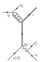
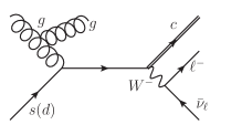
(a)

(b)

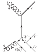
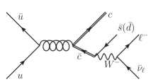
(c)

(d)

Figure 2: Examples of Feynman diagrams contributing to the real corrections for the process $pp\rightarrow\ell^{-}\bar{\nu}_{\ell}c\,j$, where $j=g,u,d,s,\bar{u},\bar{d},\bar{s}$. The last Feynman diagram (d) is an example of “regular” contribution, i.e. no singularities are associated with this process.

Together with the QCD virtual corrections to the subprocesses in Eq. (1), not depicted here, also the real corrections contribute at the next-to-leading order. Examples of Feynman diagrams contributing to the real corrections for the process $pp\rightarrow\ell^{-}\bar{\nu}_{\ell}c\,j$ are shown in Fig. 2. We can separate the real-correction contributions into two classes:

1. The corrections of the type $pp\rightarrow\ell^{-}\bar{\nu}_{\ell}\,c\,j$, with $j=g,u(\bar{u}),d(\bar{d}),s(\bar{s})$, that are singular in the limit of the unresolved jet

   $$q(\bar{q})\,s(d)\rightarrow\ell^{-}\,\bar{\nu}_{\ell}\,c\,q(\bar{q})$$

   $$g\,s(d)\rightarrow\ell^{-}\,\bar{\nu}_{\ell}\,c\,g$$ (2)

   $$g\,g\rightarrow\ell^{-}\,\bar{\nu}_{\ell}\,c\,\bar{s}(d)\,,$$

   where $q=u,d,s$. Examples of these contributions are depicted in Fig. 2, diagrams (a), (b) and (c). We will refer to these terms with $R$ in the following.

2. The corrections of the type

   $$q\,\bar{q}\rightarrow\ell^{-}\,\bar{\nu}_{\ell}\,c\,\bar{q}^{\prime},$$ (3)

   where $q=u,d,s$ and $q^{\prime}=s,d$, which do not have any singularities associated with the extra light-parton emission, and are called regular, in the POWHEG jargon and will be indicated with $R_{\rm\mathchoice{\displaystyle}{\scriptstyle}{\scriptscriptstyle}{\scriptscriptstyle}reg}$. Again we do not consider contributions with a final-state $b$ quark. An example of this type of contributions is depicted in Fig. 2 (d).

Notice that the square of the diagrams contributing to the regular processes (Fig. 2 (d)), as well as similar diagrams with two gluons in the initial state (that interfere with the one in (c)), suffer from another potential source of divergence, due to the presence of the charm anti-quark in the $s$ channel. In fact, when the invariant mass of the system comprising the $\bar{s}(\bar{d})$ quark and the two leptons is equal to the charm mass $m_{c}$, these diagrams are divergent, due to the fact that the $c$-quark propagator goes on shell. In order to avoid this singularity, we can impose a technical cut on the invariant mass of the off-shell $W$ boson

$$m_{\ell\nu}^{2}\equiv(p_{\mathchoice{\displaystyle}{\scriptstyle}{\scriptscriptstyle}{\scriptscriptstyle}\ell}+p_{\mathchoice{\displaystyle}{\scriptstyle}{\scriptscriptstyle}{\scriptscriptstyle}\nu})^{2}>m_{c}^{2}\,,$$ (4)

in the theoretical simulation. In order to make a closer contact to experimentally accessible quantities, a more realistic cut is in general imposed on the transverse mass of the $W$ system, $m_{\mathchoice{\displaystyle}{\scriptstyle}{\scriptscriptstyle}{\scriptscriptstyle}TW}$, defined as

$$m_{\mathchoice{\displaystyle}{\scriptstyle}{\scriptscriptstyle}{\scriptscriptstyle}TW}^{2}=2\,p_{\mathchoice{\displaystyle}{\scriptstyle}{\scriptscriptstyle}{\scriptscriptstyle}\perp\ell}\,p_{\mathchoice{\displaystyle}{\scriptstyle}{\scriptscriptstyle}{\scriptscriptstyle}\perp\nu}\left(1-\cos\Delta\varphi\right)\,,$$ (5)

where $\Delta\varphi$ is the azimuthal separation between the transverse momenta of the charged lepton and the missing energy of the neutrino.

We neglect contributions with two charmed quark in the final state, such as $\bar{u}d\rightarrow\ell^{-}\,\bar{\nu}_{\ell}\,c\bar{c}$, coming from the splitting $g\to c\bar{c}$, since these contributions are subtracted from experimental data in studies aimed at extracting information on the strange-quark parton distribution function, as illustrated in Sect. 4.2.

The Born and virtual matrix elements, as well as the Born colour- and spin-correlated amplitudes, necessary to the POWHEG BOX RES to automatically implement the POWHEG formalism, have been computed analytically. The one-loop amplitudes have been validated against the Gosam code Cullen:2014yla ; Cullen:2011ac . The matrix elements for the real contributions were instead generated using Madgraph4 Alwall:2007st and its interface with the POWHEG BOX Campbell:2012am .

2.1 The decoupling and $\boldsymbol{\overline{\rm MS}}$ schemes

When performing a fixed-order calculation with massive quarks, one can define al least two consistent renormalization schemes that describe the same physics: the usual $\overline{\rm MS}$ scheme, where all flavours are treated on equal footing, and a mixed scheme Collins:1978wz , called decoupling scheme Appelquist:1974tg , in which the $n_{\rm lf}$ light flavours are subtracted in the $\overline{\rm MS}$ scheme, while the heavy-flavour loop is subtracted at zero momentum. In this scheme, the heavy flavour decouples at low energies. This is the scheme we have used in the renormalization of our analytic calculation, with $n_{\rm lf}=3$.

If the decoupling scheme is chosen, then the strong coupling constant $\alpha_{\mathchoice{\displaystyle}{\scriptstyle}{\scriptscriptstyle}{\scriptscriptstyle}\rm S}$ runs with three light flavours, and the parton distribution functions should not include the charm quark in the evolution.

To make contact with other results expressed in terms of the ${\overline{\rm MS}}$ strong coupling constant, running with five light flavours, and with PDFs with five flavours, we prefer to change our renormalization scheme and to switch to the ${\overline{\rm MS}}$ one. The procedure for such a switch is well known, and was discussed in Ref. Cacciari:1998it . This procedure, applied to the $b$ quark, is also illustrated in Appendix A of Ref. Luisoni:2015mpa .

For the case under study, since the LO process contains only one power of $\alpha_{\mathchoice{\displaystyle}{\scriptstyle}{\scriptscriptstyle}{\scriptscriptstyle}\rm S}$, if we want to express our calculation in terms of a coupling constant defined in the $\overline{\rm MS}$ scheme with five active flavours, we need to add the following contribution to the cross section

$$\Delta V_{\alpha_{\mathchoice{\displaystyle}{\scriptstyle}{\scriptscriptstyle}{\scriptscriptstyle}\rm S}}(\mu_{\mathchoice{\displaystyle}{\scriptstyle}{\scriptscriptstyle}{\scriptscriptstyle}\rm R};m_{b},m_{c})=-\frac{1}{3}T_{\mathchoice{\displaystyle}{\scriptstyle}{\scriptscriptstyle}{\scriptscriptstyle}F}\frac{\alpha_{\mathchoice{\displaystyle}{\scriptstyle}{\scriptscriptstyle}{\scriptscriptstyle}\rm S}}{\pi}\left(\log\frac{\mu_{\mathchoice{\displaystyle}{\scriptstyle}{\scriptscriptstyle}{\scriptscriptstyle}\rm R}^{2}}{m_{c}^{2}}+\log\frac{\mu_{\mathchoice{\displaystyle}{\scriptstyle}{\scriptscriptstyle}{\scriptscriptstyle}\rm R}^{2}}{m_{b}^{2}}\right)B\,,$$ (6)

where $B$ is the Born cross section, $m_{b}$ the bottom mass and $\mu_{\mathchoice{\displaystyle}{\scriptstyle}{\scriptscriptstyle}{\scriptscriptstyle}\rm R}$ is the renormalization scale. A corresponding modification has to be applied if we want to employ PDFs with five active flavours. The gluon PDF, which appears in the LO cross section, induces a correction

$$\Delta V_{g}(\mu_{\mathchoice{\displaystyle}{\scriptstyle}{\scriptscriptstyle}{\scriptscriptstyle}\rm F};m_{b},m_{c})=+\frac{1}{3}T_{\mathchoice{\displaystyle}{\scriptstyle}{\scriptscriptstyle}{\scriptscriptstyle}F}\frac{\alpha_{\mathchoice{\displaystyle}{\scriptstyle}{\scriptscriptstyle}{\scriptscriptstyle}\rm S}}{\pi}\left(\log\frac{\mu_{\mathchoice{\displaystyle}{\scriptstyle}{\scriptscriptstyle}{\scriptscriptstyle}\rm F}^{2}}{m_{c}^{2}}+\log\frac{\mu_{\mathchoice{\displaystyle}{\scriptstyle}{\scriptscriptstyle}{\scriptscriptstyle}\rm F}^{2}}{m_{b}^{2}}\right)B\,,$$ (7)

where $\mu_{\mathchoice{\displaystyle}{\scriptstyle}{\scriptscriptstyle}{\scriptscriptstyle}\rm F}$ is the factorization scale. The quark PDF receives only corrections that starts at order $\alpha_{\mathchoice{\displaystyle}{\scriptstyle}{\scriptscriptstyle}{\scriptscriptstyle}\rm S}^{2}$, and can thus be neglected. By adding Eqs. (6) and (7), we get the conversion factor for the two schemes

$$\Delta V(\mu_{\mathchoice{\displaystyle}{\scriptstyle}{\scriptscriptstyle}{\scriptscriptstyle}\rm F},\mu_{\mathchoice{\displaystyle}{\scriptstyle}{\scriptscriptstyle}{\scriptscriptstyle}\rm R})=\Delta V_{\alpha_{\mathchoice{\displaystyle}{\scriptstyle}{\scriptscriptstyle}{\scriptscriptstyle}\rm S}}+\Delta V_{g}=\frac{2}{3}\,T_{\mathchoice{\displaystyle}{\scriptstyle}{\scriptscriptstyle}{\scriptscriptstyle}F}\frac{\alpha_{\mathchoice{\displaystyle}{\scriptstyle}{\scriptscriptstyle}{\scriptscriptstyle}\rm S}}{\pi}\,B\log\frac{\mu_{\mathchoice{\displaystyle}{\scriptstyle}{\scriptscriptstyle}{\scriptscriptstyle}\rm F}^{2}}{\mu_{\mathchoice{\displaystyle}{\scriptstyle}{\scriptscriptstyle}{\scriptscriptstyle}\rm R}^{2}}\,,$$ (8)

that turns out to be independent from the bottom and charm masses, and different from zero only if the renormalization and factorization scales are different.

2.2 Renormalization and factorization scale settings

In the POWHEG BOX there is the option to use a different renormalization and factorization scale when computing the real contribution (and/or the subtraction terms, i.e. their soft and collinear limits) or the Born and the virtual ones. The only requirement is that the scale used in the evaluation of the real contributions (and possibly of the subtraction terms) must tend to the scale used in the Born amplitude, when the emitted parton gets unresolved.

The default central scale used in our simulation in the evaluation of the Born, virtual, real and subtraction terms is

$$\mu=\frac{H_{\mathchoice{\displaystyle}{\scriptstyle}{\scriptscriptstyle}{\scriptscriptstyle}T}}{2}$$ (9)

with

$$H_{\mathchoice{\displaystyle}{\scriptstyle}{\scriptscriptstyle}{\scriptscriptstyle}T}=\sqrt{|\vec{p}_{\perp c}|^{2}+m_{c}^{2}}+\sqrt{|\vec{p}_{\perp\ell}+\vec{p}_{\perp\nu}|^{2}+(p_{\ell}+p_{\nu})^{2}}\,,$$ (10)

evaluated with the kinematics of the underlying-Born configuration. The regular real term $R_{\rm\mathchoice{\displaystyle}{\scriptstyle}{\scriptscriptstyle}{\scriptscriptstyle}reg}$ has no underlying Born configuration, and the scale $H_{\mathchoice{\displaystyle}{\scriptstyle}{\scriptscriptstyle}{\scriptscriptstyle}T}$ is computed using the kinematics of the real emission contribution, adding also the transverse momentum of the massless emitted parton.

$$H_{\mathchoice{\displaystyle}{\scriptstyle}{\scriptscriptstyle}{\scriptscriptstyle}T}=\sqrt{|\vec{p}_{\perp c}|^{2}+m_{c}^{2}}+\sqrt{|\vec{p}_{\perp\ell}+\vec{p}_{\perp\nu}|^{2}+(p_{\ell}+p_{\nu})^{2}}+\left|\vec{p}_{\perp j}\right|\,.$$ (11)

Other options contemplate the use of the scale (11) also in the real term and/or in the subtraction terms, or a fixed scale, such as $\mu=m_{\mathchoice{\displaystyle}{\scriptstyle}{\scriptscriptstyle}{\scriptscriptstyle}W}$.

The renormalization and factorization scales, $\mu_{\mathchoice{\displaystyle}{\scriptstyle}{\scriptscriptstyle}{\scriptscriptstyle}\rm R}$ and $\mu_{\mathchoice{\displaystyle}{\scriptstyle}{\scriptscriptstyle}{\scriptscriptstyle}\rm F}$, are defined multiplying $\mu$ by the factors $\xi_{\mathchoice{\displaystyle}{\scriptstyle}{\scriptscriptstyle}{\scriptscriptstyle}R}$ and $\xi_{\mathchoice{\displaystyle}{\scriptstyle}{\scriptscriptstyle}{\scriptscriptstyle}F}$ respectively. The uncertainty due to missing higher order corrections is estimated considering the 7-point scale variations

$$(\xi_{\mathchoice{\displaystyle}{\scriptstyle}{\scriptscriptstyle}{\scriptscriptstyle}R},\xi_{\mathchoice{\displaystyle}{\scriptstyle}{\scriptscriptstyle}{\scriptscriptstyle}F})=(1,1),\,(1,2),\,(1,0.5),\,(2,1),\,(0.5,1),\,(2,2),\,(0.5,0.5).$$ (12)

We employ the NNPDF3.1_nlo_pdfas Buckley:2014ana ; NNPDF:2017mvq PDF set, which is also used to determine the running of the strong coupling.

2.3 Numerical inputs

We have simulated $Wc$ production in $pp$ collisions at $\sqrt{s}=13$ TeV. The input parameters we have used are

$$m_{\mathchoice{\displaystyle}{\scriptstyle}{\scriptscriptstyle}{\scriptscriptstyle}W}=80.385\leavevmode\nobreak\ {\rm GeV}\phantom{{}^{-2}\times 10^{-5}}\qquad\Gamma_{\mathchoice{\displaystyle}{\scriptstyle}{\scriptscriptstyle}{\scriptscriptstyle}W}=2.085\leavevmode\nobreak\ {\rm GeV}$$

$$m_{\mathchoice{\displaystyle}{\scriptstyle}{\scriptscriptstyle}{\scriptscriptstyle}Z}=91.1876\leavevmode\nobreak\ {\rm GeV}\phantom{{}^{-2}\times 10^{-5}}\qquad\Gamma_{\mathchoice{\displaystyle}{\scriptstyle}{\scriptscriptstyle}{\scriptscriptstyle}Z}=2.4952\leavevmode\nobreak\ {\rm GeV}$$ (13)

$$G_{\mu}=1.16639\times 10^{-5}\leavevmode\nobreak\ {\rm GeV}^{-2}\,\qquad m_{c}=1.5\leavevmode\nobreak\ {\rm GeV}.$$

The electromagnetic coupling is obtained in the $G_{\mu}$ scheme

$$\alpha_{\rm em}=\frac{\sqrt{2}}{\pi}G_{\mu}m_{\mathchoice{\displaystyle}{\scriptstyle}{\scriptscriptstyle}{\scriptscriptstyle}W}^{2}\left(1-\frac{m_{\mathchoice{\displaystyle}{\scriptstyle}{\scriptscriptstyle}{\scriptscriptstyle}W}^{2}}{m_{\mathchoice{\displaystyle}{\scriptstyle}{\scriptscriptstyle}{\scriptscriptstyle}Z}^{2}}\right),$$ (14)

and the values of relevant CKM matrix elements are

$$|V_{cd}|=0.22438\,,\qquad|V_{cs}|=0.97356\,.$$ (15)

In our calculation we have neglected the mass of the leptons. Only at the stage of event generation a leptonic mass is assigned to the charged lepton once the full kinematics of the event is generated. The assignment of the mass is done through a reshuffling procedure that preserves the total energy and momentum, and the virtuality of the resonances. The values of the lepton masses we have used are given by

$$m_{e}=0.511\times 10^{-3}\leavevmode\nobreak\ {\rm GeV},\qquad m_{\mu}=0.1057\leavevmode\nobreak\ {\rm GeV},\qquad m_{\tau}=1.777\leavevmode\nobreak\ {\rm GeV}.$$ (16)

Furthermore, following the discussion that precedes Eq. (4), we always apply a technical loose cut, at the generation stage, on the $W$-boson virtuality

$$m_{\ell\nu}>2\leavevmode\nobreak\ {\rm GeV}\,.$$ (17)

2.4 Fixed-order validation

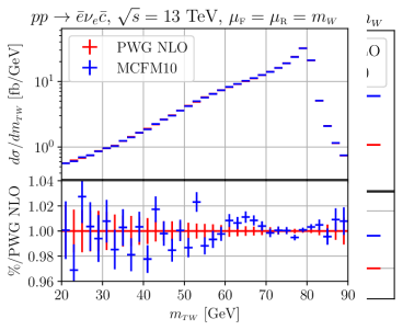
Figure 3: Differential distribution for the transverse mass of the reconstructed $W^{-}$ boson for the processes $pp\to e^{-}\bar{\nu}_{e}c$ (left) and the transverse momentum of the heavy anti-charm quark for the processes $pp\to e^{+}\nu_{e}\bar{c}$ (right) at NLO accuracy. The input parameters are discussed in Sect. 2.3. The ratio between predictions obtained with MCFM (blue) and the POWHEG BOX RES (red) is also shown. The statistical error bars from the Monte Carlo integrator are also shown.

In this section we compare our fixed-order results with those obtained with the MCFM code Campbell:2019dru ; Campbell:2015qma . In order to perform the comparison we employ a fixed renormalization and factorization scale set to

$$\mu_{\mathchoice{\displaystyle}{\scriptstyle}{\scriptscriptstyle}{\scriptscriptstyle}\rm F}=\mu_{\mathchoice{\displaystyle}{\scriptstyle}{\scriptscriptstyle}{\scriptscriptstyle}\rm R}=m_{\mathchoice{\displaystyle}{\scriptstyle}{\scriptscriptstyle}{\scriptscriptstyle}W}\,.$$ (18)

As we are setting $\mu_{\mathchoice{\displaystyle}{\scriptstyle}{\scriptscriptstyle}{\scriptscriptstyle}\rm F}=\mu_{\mathchoice{\displaystyle}{\scriptstyle}{\scriptscriptstyle}{\scriptscriptstyle}\rm R}$, the term $\Delta{\rm V}$ defined in Eq. (8) vanishes and there is no correction factor. We define the fiducial cross section imposing the following cuts on the transverse momentum and rapidity of the charged lepton, as well on the transverse momentum of the charm quark

$$|\vec{p}_{\perp\ell}|>26\leavevmode\nobreak\ {\rm GeV},\qquad|y_{\ell}|<2.4\,,\qquad|\vec{p}_{\perp c}|>5\leavevmode\nobreak\ {\rm GeV}.$$ (19)

These cuts corresponds to the ones employed by the CMS Collaboration to define the inclusive cross section in the analysis described in Ref. CMS:2018dxg at $\sqrt{s}=13$ TeV.

As discussed in Sect. 2, around Eqs. (4) and (5), in order to avoid the charm-propagator singularity in diagrams like the one in Fig. 2 (d), we also implement a cut on the transverse mass of the $W$ system

$$m_{\mathchoice{\displaystyle}{\scriptstyle}{\scriptscriptstyle}{\scriptscriptstyle}TW}>20\leavevmode\nobreak\ {\rm GeV}.$$ (20)

In Table 1

$\sigma$ [fb]	$e^{-}\bar{\nu}_{e}c$ @ LO	$e^{+}\nu_{e}\bar{c}$ @ LO	$e^{-}\bar{\nu}_{e}c$ @ NLO	$e^{+}\nu_{e}\bar{c}$ @ NLO
PWG RES	352.7(1)	341.1(1)	497.2(2)	480.8(2)
MCFM 10	352.9(2)	341.2(2)	497.0(2)	481.0(3)
Ratio	1.0005(5)	1.0002(5)	0.9996(7)	1.0004(7)

Table 1: Fiducial cross section obtained with MCFM and our generator (PWG RES) for the processes $pp\to e^{-}\bar{\nu}_{e}c$ and $e^{+}\nu_{e}\bar{c}$ at LO (left columns) and NLO (right columns) at $\sqrt{s}=13$ TeV within the fiducial cuts of Eqs. (19) and (20), with $\mu_{\mathchoice{\displaystyle}{\scriptstyle}{\scriptscriptstyle}{\scriptscriptstyle}\rm F}=\mu_{\mathchoice{\displaystyle}{\scriptstyle}{\scriptscriptstyle}{\scriptscriptstyle}\rm R}=m_{\mathchoice{\displaystyle}{\scriptstyle}{\scriptscriptstyle}{\scriptscriptstyle}W}$. The input parameters are discussed in Sect. 2.3. In the last row we show the ratio between the MCFM and the POWHEG BOX RES predictions.

we show the integrated cross section at LO and NLO obtained with our code and with MCFM. In all cases a sub-permille agreement is found. Good agreement is found also at the differential level, as it can be seen in Fig. 3, where we illustrated the transverse mass of the reconstructed $W$ boson (left panel) and the transverse momentum of the charmed quark (right panel).

3 Details of the POWHEG matching

In this section we briefly recall the expression for the differential cross section generated with the POWHEG method Nason:2004rx for the process under consideration, focusing for simplicity only on the $pp\to\ell\bar{\nu}_{\ell}c$ signature, in order to discuss further sources of theoretical uncertainty intrinsic to the POWHEG method.

The NLO cross section reads

$${\rm d}\sigma_{\rm\mathchoice{\displaystyle}{\scriptstyle}{\scriptscriptstyle}{\scriptscriptstyle}NLO}=B(\Phi_{3};\mu_{\mathchoice{\displaystyle}{\scriptstyle}{\scriptscriptstyle}{\scriptscriptstyle}\rm R},\mu_{\mathchoice{\displaystyle}{\scriptstyle}{\scriptscriptstyle}{\scriptscriptstyle}\rm F})\,{\rm d}\Phi_{3}+\frac{\alpha_{\mathchoice{\displaystyle}{\scriptstyle}{\scriptscriptstyle}{\scriptscriptstyle}\rm S}(\mu_{\mathchoice{\displaystyle}{\scriptstyle}{\scriptscriptstyle}{\scriptscriptstyle}\rm R})}{2\pi} \left[V(\Phi_{3};\mu_{\mathchoice{\displaystyle}{\scriptstyle}{\scriptscriptstyle}{\scriptscriptstyle}\rm R},\mu_{\mathchoice{\displaystyle}{\scriptstyle}{\scriptscriptstyle}{\scriptscriptstyle}\rm F})\,{\rm d}\Phi_{3}+R(\Phi_{3+1};\mu_{\mathchoice{\displaystyle}{\scriptstyle}{\scriptscriptstyle}{\scriptscriptstyle}\rm R},\mu_{\mathchoice{\displaystyle}{\scriptstyle}{\scriptscriptstyle}{\scriptscriptstyle}\rm F})\,{\rm d}\Phi_{3+1}\right.$$

$$\left.{}+R_{\rm\mathchoice{\displaystyle}{\scriptstyle}{\scriptscriptstyle}{\scriptscriptstyle}reg}(\Phi_{3+1};\mu_{\mathchoice{\displaystyle}{\scriptstyle}{\scriptscriptstyle}{\scriptscriptstyle}\rm R},\mu_{\mathchoice{\displaystyle}{\scriptstyle}{\scriptscriptstyle}{\scriptscriptstyle}\rm F})\,{\rm d}\Phi_{3+1}\right],$$ (21)

where $B$, $V$, $R$ and $R_{\rm\mathchoice{\displaystyle}{\scriptstyle}{\scriptscriptstyle}{\scriptscriptstyle}reg}$ are the Born, virtual, real and regular real matrix elements, multiplied by the appropriate PDF and flux factors. As stated in Sect. 2, we indicate with $R_{\rm\mathchoice{\displaystyle}{\scriptstyle}{\scriptscriptstyle}{\scriptscriptstyle}reg}$ the terms arising from the flavour configurations of Eq. (3), which do not contain any QCD singularity, while the processes in Eq. (1) are designated with $R$. The Born and virtual cross sections are evaluated using a three-body phase space $\Phi_{3}$, while, in the real contributions, an additional light parton is present. The matrix elements depend on the $\mu_{\mathchoice{\displaystyle}{\scriptstyle}{\scriptscriptstyle}{\scriptscriptstyle}\rm R}$ scale, as the LO starts with one power of the strong coupling constant $\alpha_{\mathchoice{\displaystyle}{\scriptstyle}{\scriptscriptstyle}{\scriptscriptstyle}\rm S}$, while the $\mu_{\mathchoice{\displaystyle}{\scriptstyle}{\scriptscriptstyle}{\scriptscriptstyle}\rm F}$ dependence arises from the incoming-parton PDFs. To build the POWHEG cross section, the real term $R$ is split into a singular $R_{\mathchoice{\displaystyle}{\scriptstyle}{\scriptscriptstyle}{\scriptscriptstyle}s}$ and a finite contribution $R_{\mathchoice{\displaystyle}{\scriptstyle}{\scriptscriptstyle}{\scriptscriptstyle}f}$, and the $\bar{B}$ term is defined as

$$\bar{B}(\Phi_{3};\mu_{\mathchoice{\displaystyle}{\scriptstyle}{\scriptscriptstyle}{\scriptscriptstyle}\rm F},\mu_{\mathchoice{\displaystyle}{\scriptstyle}{\scriptscriptstyle}{\scriptscriptstyle}\rm R})=B(\Phi_{3};\mu_{\mathchoice{\displaystyle}{\scriptstyle}{\scriptscriptstyle}{\scriptscriptstyle}\rm R},\mu_{\mathchoice{\displaystyle}{\scriptstyle}{\scriptscriptstyle}{\scriptscriptstyle}\rm F})+\frac{\alpha_{\mathchoice{\displaystyle}{\scriptstyle}{\scriptscriptstyle}{\scriptscriptstyle}\rm S}(\mu_{\mathchoice{\displaystyle}{\scriptstyle}{\scriptscriptstyle}{\scriptscriptstyle}\rm R})}{2\pi}\left[V(\Phi_{3};\mu_{\mathchoice{\displaystyle}{\scriptstyle}{\scriptscriptstyle}{\scriptscriptstyle}\rm R},\mu_{\mathchoice{\displaystyle}{\scriptstyle}{\scriptscriptstyle}{\scriptscriptstyle}\rm F})+\int d\Phi_{1}\,R_{\mathchoice{\displaystyle}{\scriptstyle}{\scriptscriptstyle}{\scriptscriptstyle}s}(\Phi_{3+1};\mu_{\mathchoice{\displaystyle}{\scriptstyle}{\scriptscriptstyle}{\scriptscriptstyle}\rm R},\mu_{\mathchoice{\displaystyle}{\scriptstyle}{\scriptscriptstyle}{\scriptscriptstyle}\rm F})\right],$$ (22)

where $\Phi_{1}$ is the radiation phase space, defined in terms of three radiation variables. The probability of not having any resolved emissions up to a scale $k_{\mathchoice{\displaystyle}{\scriptstyle}{\scriptscriptstyle}{\scriptscriptstyle}\rm T}^{\prime}$ is given by

$$\Delta_{\mathchoice{\displaystyle}{\scriptstyle}{\scriptscriptstyle}{\scriptscriptstyle}s}(k_{\mathchoice{\displaystyle}{\scriptstyle}{\scriptscriptstyle}{\scriptscriptstyle}\rm T}^{\prime};\Phi_{3})=\exp\left[-\int{\rm d}\Phi_{1}\,\theta\!\left[k_{\mathchoice{\displaystyle}{\scriptstyle}{\scriptscriptstyle}{\scriptscriptstyle}\rm T}(\Phi_{1})-k_{\mathchoice{\displaystyle}{\scriptstyle}{\scriptscriptstyle}{\scriptscriptstyle}\rm T}^{\prime}\right]\frac{\alpha_{\mathchoice{\displaystyle}{\scriptstyle}{\scriptscriptstyle}{\scriptscriptstyle}\rm S}(k_{\mathchoice{\displaystyle}{\scriptstyle}{\scriptscriptstyle}{\scriptscriptstyle}\rm T})}{2\pi}\,\frac{{R}_{\mathchoice{\displaystyle}{\scriptstyle}{\scriptscriptstyle}{\scriptscriptstyle}s}(\Phi_{3+1};k_{\mathchoice{\displaystyle}{\scriptstyle}{\scriptscriptstyle}{\scriptscriptstyle}\rm T},k_{\mathchoice{\displaystyle}{\scriptstyle}{\scriptscriptstyle}{\scriptscriptstyle}\rm T})}{{B}(\Phi_{3};k_{\mathchoice{\displaystyle}{\scriptstyle}{\scriptscriptstyle}{\scriptscriptstyle}\rm T},k_{\mathchoice{\displaystyle}{\scriptstyle}{\scriptscriptstyle}{\scriptscriptstyle}\rm T})}\right],$$ (23)

where the factorization and the renormalization scales are evaluated at the scale $k_{\mathchoice{\displaystyle}{\scriptstyle}{\scriptscriptstyle}{\scriptscriptstyle}\rm T}$, which corresponds to the transverse momentum of the light parton, if it is collinear to an initial-state parton, while, for gluon emissions from the final-state charm quark, it is given by

$$k_{\mathchoice{\displaystyle}{\scriptstyle}{\scriptscriptstyle}{\scriptscriptstyle}\rm T}^{2}=2\frac{E_{g}}{E_{c}}\left(p_{g}\cdot p_{c}\right),$$ (24)

where $p_{g}$ and $p_{c}$ are the gluon and charm four-momenta and $E_{g}$ and $E_{c}$ their energies in the partonic center-of-mass frame.

The POWHEG cross section finally reads

$${\rm d}\sigma_{{\rm\mathchoice{\displaystyle}{\scriptstyle}{\scriptscriptstyle}{\scriptscriptstyle}PWG}}= \bar{B}(\Phi_{3};\mu_{\mathchoice{\displaystyle}{\scriptstyle}{\scriptscriptstyle}{\scriptscriptstyle}\rm F},\mu_{\mathchoice{\displaystyle}{\scriptstyle}{\scriptscriptstyle}{\scriptscriptstyle}\rm R})\,{\rm d}\Phi_{3}\left[\frac{\alpha_{\mathchoice{\displaystyle}{\scriptstyle}{\scriptscriptstyle}{\scriptscriptstyle}\rm S}(k_{\mathchoice{\displaystyle}{\scriptstyle}{\scriptscriptstyle}{\scriptscriptstyle}\rm T})}{2\pi}\frac{R_{\mathchoice{\displaystyle}{\scriptstyle}{\scriptscriptstyle}{\scriptscriptstyle}s}(\Phi_{3+1};k_{\mathchoice{\displaystyle}{\scriptstyle}{\scriptscriptstyle}{\scriptscriptstyle}\rm T},k_{\mathchoice{\displaystyle}{\scriptstyle}{\scriptscriptstyle}{\scriptscriptstyle}\rm T})}{{B}(\Phi_{3};k_{\mathchoice{\displaystyle}{\scriptstyle}{\scriptscriptstyle}{\scriptscriptstyle}\rm T},k_{\mathchoice{\displaystyle}{\scriptstyle}{\scriptscriptstyle}{\scriptscriptstyle}\rm T})}\,\Delta_{\mathchoice{\displaystyle}{\scriptstyle}{\scriptscriptstyle}{\scriptscriptstyle}s}(k_{\mathchoice{\displaystyle}{\scriptstyle}{\scriptscriptstyle}{\scriptscriptstyle}\rm T};\Phi_{3})\,{\rm d}\Phi_{1}+\Delta_{\mathchoice{\displaystyle}{\scriptstyle}{\scriptscriptstyle}{\scriptscriptstyle}s}(k_{\mathchoice{\displaystyle}{\scriptstyle}{\scriptscriptstyle}{\scriptscriptstyle}\rm T}^{\mathchoice{\displaystyle}{\scriptstyle}{\scriptscriptstyle}{\scriptscriptstyle}\rm min};\Phi_{3})\right]$$

$$+\frac{\alpha_{\mathchoice{\displaystyle}{\scriptstyle}{\scriptscriptstyle}{\scriptscriptstyle}\rm S}(\mu_{\mathchoice{\displaystyle}{\scriptstyle}{\scriptscriptstyle}{\scriptscriptstyle}\rm R})}{2\pi}R_{\mathchoice{\displaystyle}{\scriptstyle}{\scriptscriptstyle}{\scriptscriptstyle}f}(\Phi_{3+1};\mu_{\mathchoice{\displaystyle}{\scriptstyle}{\scriptscriptstyle}{\scriptscriptstyle}\rm R},\mu_{\mathchoice{\displaystyle}{\scriptstyle}{\scriptscriptstyle}{\scriptscriptstyle}\rm F})\,{\rm d}\Phi_{3+1}+\frac{\alpha_{\mathchoice{\displaystyle}{\scriptstyle}{\scriptscriptstyle}{\scriptscriptstyle}\rm S}(\mu_{\mathchoice{\displaystyle}{\scriptstyle}{\scriptscriptstyle}{\scriptscriptstyle}\rm R})}{2\pi}R_{\rm\mathchoice{\displaystyle}{\scriptstyle}{\scriptscriptstyle}{\scriptscriptstyle}reg}(\Phi_{3+1};\mu_{\mathchoice{\displaystyle}{\scriptstyle}{\scriptscriptstyle}{\scriptscriptstyle}\rm R},\mu_{\mathchoice{\displaystyle}{\scriptstyle}{\scriptscriptstyle}{\scriptscriptstyle}\rm F})\,{\rm d}\Phi_{3+1}\,,$$ (25)

where $k_{\mathchoice{\displaystyle}{\scriptstyle}{\scriptscriptstyle}{\scriptscriptstyle}\rm T}^{\mathchoice{\displaystyle}{\scriptstyle}{\scriptscriptstyle}{\scriptscriptstyle}\rm min}$ is an infrared cutoff.

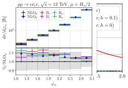
Figure 4: Comparison of three damping functions used to separate the real contribution into a singular and a finite part, as detailed in Sect. 3.

There are several degrees of freedom in the implementation of Eq. (3). One of them is in the choice of the renormalization and factorization scales $\mu_{\mathchoice{\displaystyle}{\scriptstyle}{\scriptscriptstyle}{\scriptscriptstyle}\rm R}$ and $\mu_{\mathchoice{\displaystyle}{\scriptstyle}{\scriptscriptstyle}{\scriptscriptstyle}\rm F}$ in the $R_{\mathchoice{\displaystyle}{\scriptstyle}{\scriptscriptstyle}{\scriptscriptstyle}f}$ and $R_{\rm\mathchoice{\displaystyle}{\scriptstyle}{\scriptscriptstyle}{\scriptscriptstyle}reg}$ terms, as well as in the term $R_{\mathchoice{\displaystyle}{\scriptstyle}{\scriptscriptstyle}{\scriptscriptstyle}s}$ appearing in $\bar{B}$ in Eq. (22), as discussed in Sect. 2.2. Another one is in the choice of how to separate $R$ into a singular part $R_{\mathchoice{\displaystyle}{\scriptstyle}{\scriptscriptstyle}{\scriptscriptstyle}s}$ and a finite one $R_{\mathchoice{\displaystyle}{\scriptstyle}{\scriptscriptstyle}{\scriptscriptstyle}f}$. Without loss of generality, one can separate the two contributions introducing what is called a “damping function”, $f(k_{\mathchoice{\displaystyle}{\scriptstyle}{\scriptscriptstyle}{\scriptscriptstyle}\rm T})$, that satisfies

$$0\leq f(k_{\mathchoice{\displaystyle}{\scriptstyle}{\scriptscriptstyle}{\scriptscriptstyle}\rm T})\leq 1\,,\qquad\lim_{k_{\mathchoice{\displaystyle}{\scriptstyle}{\scriptscriptstyle}{\scriptscriptstyle}\rm T}\to 0}f(k_{\mathchoice{\displaystyle}{\scriptstyle}{\scriptscriptstyle}{\scriptscriptstyle}\rm T})=1$$ (26)

and define

$$R_{\mathchoice{\displaystyle}{\scriptstyle}{\scriptscriptstyle}{\scriptscriptstyle}s}=f(k_{\mathchoice{\displaystyle}{\scriptstyle}{\scriptscriptstyle}{\scriptscriptstyle}\rm T})\,R,\qquad R_{\mathchoice{\displaystyle}{\scriptstyle}{\scriptscriptstyle}{\scriptscriptstyle}f}=\left[1-f(k_{\mathchoice{\displaystyle}{\scriptstyle}{\scriptscriptstyle}{\scriptscriptstyle}\rm T})\right]R\,.$$ (27)

For the process we are studying, we have considered two different forms for $f$

$$f_{1}(x)= \hskip 5.69046pt\frac{1}{1+x^{2}}$$ (28)

$$f_{2}(x;h)= \begin{cases}1\quad&\mbox{ for }x\leq 1-2h\\ {\displaystyle 1-\frac{(1-2h-x)^{2}}{2h^{2}}}&\mbox{ for }1-2h<x\leq 1-h\\[5.69054pt] {\displaystyle\frac{(1-x)^{2}}{2h^{2}}}&\mbox{ for }1-h<x\leq 1\\[5.69054pt] 0&\mbox{ for }x>1,\end{cases}$$ (29)

with

$$x=\frac{1}{\mu}\sqrt{k_{\mathchoice{\displaystyle}{\scriptstyle}{\scriptscriptstyle}{\scriptscriptstyle}\rm T}^{2}-m_{c}^{2}}\,\,\theta\!\left(k_{\mathchoice{\displaystyle}{\scriptstyle}{\scriptscriptstyle}{\scriptscriptstyle}\rm T}-m_{c}\right),$$ (30)

where $\mu$ is defined in Eq. (9), and $0\leq h\leq 1/2$ is a free parameter. The value of $x$ is set to 0 if $k_{\mathchoice{\displaystyle}{\scriptstyle}{\scriptscriptstyle}{\scriptscriptstyle}\rm T}<m_{c}$, so that no finite contribution is present with $k_{\mathchoice{\displaystyle}{\scriptstyle}{\scriptscriptstyle}{\scriptscriptstyle}\rm T}$ below the charm mass. The functional form $f_{2}$ in Eq. (29), with $h=0.3$, is the default damping function in the Herwig7.2 event generator Bellm:2016rhh , while $f_{1}$ in Eq. (28) corresponds to the default option of the POWHEG BOX RES. In Fig. 4 we provide a graphical representation of $f_{1}$, $f_{2}(h=0.1)$ and $f_{2}(h=0)$.

acronym	scales in $R$	damping function $f$
B0	underlying-Born kinematics	1
B1	underlying-Born kinematics	$f_{1}$
B2	underlying-Born kinematics	$f_{2}(h=0.1)$
R0	real kinematics	1

Table 2: Setups for the implementation of the POWHEG cross section given in Eq. (3). The second column denotes the kinematic configuration used to evaluate the renormalization and factorization scales in the computation of the real and subtraction terms, while the last column shows which profile function is used to evaluate Eq. (27). The functional forms of $f_{1}$ and $f_{2}$ are given in Eqs. (28) and (29) respectively.

In the following we investigate the dependence of several inclusive (with respect to the QCD radiation) observables, such as the leptonic observables and the rapidity and the transverse momentum of the jet containing the charm quark.

We reconstruct jets using the Fastjet Cacciari:2011ma implementation of the anti-$k_{\mathchoice{\displaystyle}{\scriptstyle}{\scriptscriptstyle}{\scriptscriptstyle}\rm T}$ algorithm Cacciari:2008gp with $R=0.5$. To this aim, we have considered the setups listed in Table 2 to compute the POWHEG cross section given in Eq. (3). The central value of the renormalization and factorization scales is set to $H_{\mathchoice{\displaystyle}{\scriptstyle}{\scriptscriptstyle}{\scriptscriptstyle}T}/2$ (see Eq. (9)).

In the following figures we will compare some kinematic distributions computed with six different setups: two fixed-order NLO results, one computed using the underlying-Born kinematics (NLO_B) for the renormalization and factorization scale in the real contributions, and the other one using the full real-event kinematics, indicated with NLO_R. The other four distributions are computed analysing the POWHEG-generated events at the “Les Houches” (LHE) level, i.e. events with the first hardest radiation generated according to Eq. (3), adopting the setup scales and damping functions of Table 2. For inclusive observables, the LHE results should agree with the fixed-order NLO ones up to NNLO terms.

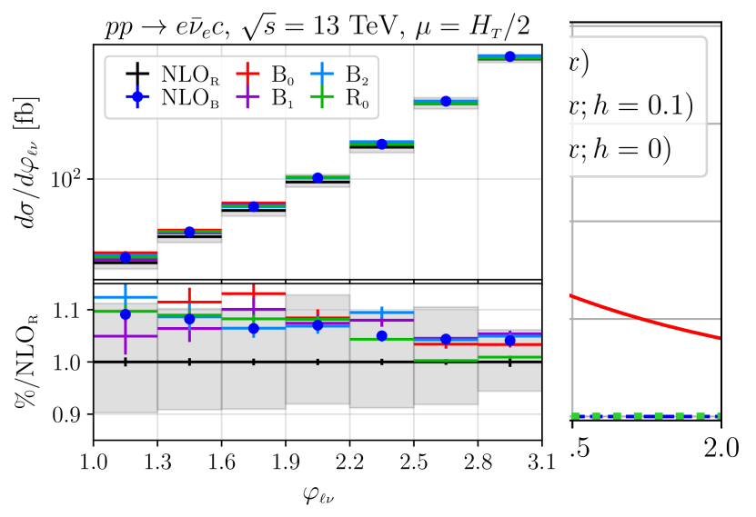
Figure 5: The transverse mass distribution of the reconstructed $W$ boson (left) and the rapidity of the charmed jet (right) at NLO (NLO_B and NLO_R) and at the Les Houches event level, for the choices of the scales and damping functions listed in Table 2. The grey bands are obtained performing the 7-point scale variations in Eq. (12) of the NLO_R results. The statistical errors from the integration procedure are also shown.

In Fig. 5 we plot the transverse mass of the $W$ boson (left panel) and the rapidity of the charmed jet (right panel). The NLO_B results (blue line) are roughly 3% higher than the NLO_R ones (black line), although always contained in the grey scale-uncertainty band of NLO_R, computed performing the 7-point scale variations in Eq. (12). Furthermore, all the distributions at the LHE level agree with the corresponding fixed order calculation, within the scale-variation band.

Figure 6: Same as Fig. 5 but for the transverse momentum of the reconstructed $W$ boson (left) and of the charmed jet (right).

The transverse momentum of the $W$ boson, $p_{\mathchoice{\displaystyle}{\scriptstyle}{\scriptscriptstyle}{\scriptscriptstyle}\perp W}$, and of the charmed jet, $p_{\mathchoice{\displaystyle}{\scriptstyle}{\scriptscriptstyle}{\scriptscriptstyle}\perp j_{c}}$, are illustrated on the left and right panel of Fig. 6, respectively. Comparing the two NLO predictions computed with different scales, one can see that the use of the underlying-Born scales favours a harder spectrum, although the result always lies within the scale-variation band of the NLO_R one, except for the very last bin. This is due to the fact that, for large $c$-jet transverse momentum, it is quite likely to produce a $c\to cg$ splitting that enhances the value of $H_{\mathchoice{\displaystyle}{\scriptstyle}{\scriptscriptstyle}{\scriptscriptstyle}T}$. As such, the underlying-Born kinematics yields a lower scale and hence a larger value for $\alpha_{\mathchoice{\displaystyle}{\scriptstyle}{\scriptscriptstyle}{\scriptscriptstyle}\rm S}$, that enhances the cross section. The same behaviour can be seen also at the LHE level.

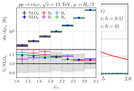
Figure 7: Same as Fig. 5 but for the transverse momentum (left) and rapidity (right) of the charged lepton, with the cuts in Eq. (19) and (20) in place.

In the experimental analyses, such as the one in Ref. CMS:2018dxg , an important role is played by the measurement of the transverse momentum and rapidity of the charged lepton. In Fig. 7 we then plot these quantities, after applying the cuts of Eq. (19), that are the same as those used by the CMS Collaboration, as well as a cut on $m_{\mathchoice{\displaystyle}{\scriptstyle}{\scriptscriptstyle}{\scriptscriptstyle}TW}$, defined in Eq. (20). As far as the fixed-order NLO results is concerned, the NLO_B curves lie a few percent above the NLO_R one, both for the transverse momentum and the rapidity. This is again due to the higher value of $\alpha_{\mathchoice{\displaystyle}{\scriptstyle}{\scriptscriptstyle}{\scriptscriptstyle}\rm S}$ when the renormalization scale is evaluated with the underlying-Born kinematics. Differences up to 10% can also be seen among the LHE curves, but, in general, all these curves lie within the grey uncertainty band of the NLO_R result, so that they are consistent among each other.

We thus conclude that no significant differences are found among the several damping factors, particularly when realistic analysis cuts are applied, and that the main theoretical uncertainties arise from scale variations.

4 NLO + parton-shower results

In this section, we present full results after the completion of the POWHEG shower performed by general-purpose Monte Carlo (MC) programs, such as Herwig7.2 Bahr:2008pv ; Bellm:2019zci and Pythia8.3 Sjostrand:2006za ; Sjostrand:2014zea , including hadronization and underlying-event effects.

We have showered the Les Houches events that we have produced using the POWHEG BOX RES code, employing the Herwig7.2 angular-ordered shower (that we label as “QTilde” shower), and the default Pythia8.3 shower with fully local recoil Cabouat:2017rzi (that we denote as “Dipole” shower), as well as the Pythia implementation of the Vincia shower Brooks:2020upa ; Skands:2020lkd .

For all the different types of shower we use the default setting of their parameters, and we only change the charm mass to agree with the value we have used to generate the $Wc$ sample (see Eq.(2.3)). In Sect. 4.1 we provide additional details of the showers we have employed, while in Sect. 4.2 we investigate the impact of several ingredients provided by the general-purpose MC generators on the simulation of $Wc$ events. Finally, in Sect. 4.3 we compare our results against the experimental data at $\sqrt{s}=13$ GeV, taken by the CMS Collaboration.

4.1 The POWHEG BOX RES matching with Herwig7.2 and Pythia8.3

4.1.1 QTilde shower

The relevant parameters to shower the POWHEG-generated events with the QTilde shower are taken from the LHE-POWHEG.in input card distributed in the public release of the Herwig7.2 code. In particular the options

set /Herwig/Shower/ShowerHandler:MaxPtIsMuF Yes
set /Herwig/Shower/ShowerHandler:RestrictPhasespace Yes

instruct the shower to veto all the emissions with transverse momentum larger than the scalup variable, which is the hardness of the POWHEG emission. We set the charm mass to $1.5$ GeV

set /Herwig/Particle/c:NominalMass 1.5*GeV
set /Herwig/Particle/cbar:NominalMass 1.5*GeV

and we switch off the decay of unstable hadrons, in order to analyse more quickly the generated events

set LesHouchesHandler:DecayHandler NULL

By default, the QTilde shower includes also QED emissions, that can be switched off with the option

set /Herwig/Shower/ShowerHandler:Interactions QCD

The running coupling is evaluated at two loops in the Catani-Marchesini-Webber scheme Catani:1990rr , with $\alpha_{\mathchoice{\displaystyle}{\scriptstyle}{\scriptscriptstyle}{\scriptscriptstyle}\rm S}^{\rm\mathchoice{\displaystyle}{\scriptstyle}{\scriptscriptstyle}{\scriptscriptstyle}CMW}(m_{\mathchoice{\displaystyle}{\scriptstyle}{\scriptscriptstyle}{\scriptscriptstyle}Z})=0.1186$.

4.1.2 Dipole shower

We also considered the Pythia8.3 implementation of a dipole shower with a fully local recoil Cabouat:2017rzi

SpaceShower:dipoleRecoil = on

We employed the PowhegHooks class to veto emissions harder than the POWHEG one, all the options correspond to the default ones, present in the main31.cmnd input card in the public release of the Pythia8.3 code. To generate only the QCD shower, we set

SpaceShower:QEDshowerByQ = off
SpaceShower:QEDshowerByL = off
TimeShower:QEDshowerByQ = off
TimeShower:QEDshowerByL = off
TimeShower:QEDshowerByGamma = off
TimeShower:QEDshowerByOther  = off

and the hadrons decay is turned off with the flag

HadronLevel:Decay = off

The running coupling is evaluated at one loop in the $\overline{\rm MS}$ scheme, and $\alpha_{\mathchoice{\displaystyle}{\scriptstyle}{\scriptscriptstyle}{\scriptscriptstyle}\rm S}^{\rm\mathchoice{\displaystyle}{\scriptstyle}{\scriptscriptstyle}{\scriptscriptstyle}\overline{MS}}(m_{\mathchoice{\displaystyle}{\scriptstyle}{\scriptscriptstyle}{\scriptscriptstyle}Z})=0.140$.

4.1.3 Vincia shower

At difference with respect to the Dipole shower, Vincia is an antenna shower. To use its implementation in Pythia8.3, we set

PartonShowers:model = 2

To properly include charm-mass effects, one has to include the option

Vincia:nFlavZeroMass = 3

as, by default, this number is set to 4, meaning that only top and bottom are treated as massive. The QED shower can be turned off with the option

Vincia:ewMode = 0

The running coupling is evaluated at two loops in the Catani-Marchesini-Webber scheme, and $\alpha_{\mathchoice{\displaystyle}{\scriptstyle}{\scriptscriptstyle}{\scriptscriptstyle}\rm S}^{\rm\mathchoice{\displaystyle}{\scriptstyle}{\scriptscriptstyle}{\scriptscriptstyle}CMW}(m_{\mathchoice{\displaystyle}{\scriptstyle}{\scriptscriptstyle}{\scriptscriptstyle}Z})=0.127$. Also in this case, we use the PowhegHooks class to avoid to generate emissions harder than the POWHEG one and we do not include the unstable hadrons decay in our simulation.

4.2 NLO + PS results with hadronization and underlying-event effects

In this section we discuss the impact of the parton shower, of the hadronization and of the underlying events on the results generated using our simulation in the POWHEG BOX RES. The results presented in this section do not include the QED shower.

We focus on the $\mu^{+}\nu_{\mu}\bar{c}$ signature at $\sqrt{s}=13$ TeV. We use the values of the parameters described in Sect. 2.3, and the B₂ setting of Table 2, i.e. the central values for the renormalization and factorization scales are computed using the underlying-Born kinematics, according to Eq. (10), and as damping function we use the $f_{2}$ profile function of Eq. (29) with $h=0.1$.

We begin by analyzing the effect of the parton shower on the POWHEG BOX distributions (PWG). If, at the end of the shower, an event contains more than one muon (or anti-muon) passing the charged leptonic cuts, only the hardest one is considered to reconstruct the $W$ kinematics.

Since the aim of our analysis is to enhance the sensitivity of the measured cross section to the strange quark PDF, we proceed as follows: if more than one $c$ quark or charmed hadron is present, they are all considered, with the exception of hadrons containing a $c\bar{c}$ pair, which are counted as not charmed. In addition, when in an event the charmed-quark and the muon charges have the same sign (SS), the weight of the event is subtracted from the differential cross sections, while, when they have opposite sign (OS), the weight is added. This procedure effectively removes the background due to events where the final-state charm comes from gluon splitting $g\to c\bar{c}$, and not from an initial-state strange quark emitting a $W$ boson. Charmed quarks originated from the gluon splitting have the same probability to be SS or OS, so their contribution cancels, when the above procedure is applied.

Jets are reconstructed using the anti-$k_{\mathchoice{\displaystyle}{\scriptstyle}{\scriptscriptstyle}{\scriptscriptstyle}\rm T}$ algorithm with $R=0.5$. The charm content of a jet is defined as $N_{c}-N_{\bar{c}}$, being $N_{c}$($N_{\bar{c}}$) the number of $c$($\bar{c}$) quarks clustered in the jet, and the event weight that we use to fill a jet-related distribution is further weighted by the factor $\pm(N_{c}-N_{\bar{c}})$, where we use the $+$ sign when the muon has negative charge, and the $-$ sign otherwise.

In the following, we consider both inclusive results (with the technical cut on the $W$ boson virtuality of Eq. (17) always in place), as well as more exclusive ones, where we apply the following acceptance cuts

$$|\eta_{\mu}|<2.4\,,\quad p_{\mathchoice{\displaystyle}{\scriptstyle}{\scriptscriptstyle}{\scriptscriptstyle}\perp\mu}>26\leavevmode\nobreak\ {\rm GeV},\quad m_{\mathchoice{\displaystyle}{\scriptstyle}{\scriptscriptstyle}{\scriptscriptstyle}TW}>20\leavevmode\nobreak\ {\rm GeV},\quad|\eta_{c}|<2.4\,,\quad p_{\mathchoice{\displaystyle}{\scriptstyle}{\scriptscriptstyle}{\scriptscriptstyle}\perp c}>5\leavevmode\nobreak\ {\rm GeV},$$ (31)

used by the CMS Collaboration in their analyses.

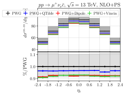
Figure 8: Effect of three different parton showers (QTilde in blue, Dipole in red and Vincia in green) on the events produced with the POWHEG BOX RES (PWG), in black, for the transverse momentum of the charmed quark (left panel) and of the charmed jet (right panel), for inclusive cuts. The grey band corresponds to the scale variations of the PWG distribution.

At the inclusive level, the parton shower acts non-trivially on the transverse-momentum distribution of the charm quark and of the charmed jet, as portrayed in Fig. 8. In particular, one can notice that the hard tail is depleted, and the region around 5 GeV is instead increased. The effect is milder for the $c$-jet, as radiation inside the cone with jet radius $R=0.5$ is still collected in the jet, but more evident for the hadron: in fact, in the high transverse-momentum region, the ratio of the LHE results with the showered ones reaches values around 50% for the quark/hadron, and 10% for the charmed jet.

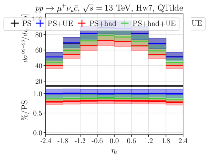
Figure 9: Effect of the underlying event (UE) and of the hadronization (had) on the NLO+PS distributions obtained with the Herwig7.2 QTilde shower for the transverse-momentum distribution of the charmed quark (left panel) and of the charmed jet (right panel) for inclusive cuts. The grey band corresponds to renormalization- and factorization-scale variation, obtained using the standard reweighting procedure implemented in the POWHEG BOX RES framework.

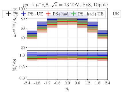
Figure 10: Same as Fig. 9, but for the Pythia8.3 Dipole shower.

In order to be able to compare theoretical predictions with data, we also have to include hadronization corrections and the simulation of the underlying-event (UE) production. In Figs. 9 and 10 we illustrate their effect on the NLO+PS distributions obtained with the Herwig7.2 QTilde shower, in Fig. 9, and with the Pythia8.3 Dipole shower, in Fig. 10. In all cases we notice that the UE have a small impact on the charmed-quark distribution, except in the region $p_{\mathchoice{\displaystyle}{\scriptstyle}{\scriptscriptstyle}{\scriptscriptstyle}\perp c}<10$ GeV. On the other hand, the underlying event hardens the $c$-jet distribution as it provides further particles that can be clustered in the jet. Hadronization corrections are large (up to 50%) and they soften the $p_{\mathchoice{\displaystyle}{\scriptstyle}{\scriptscriptstyle}{\scriptscriptstyle}\perp}$ of the charmed quark/hadron. Similar, but milder effects are seen for the charmed jet.

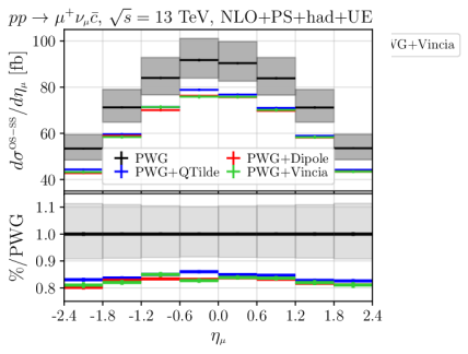
Figure 11: Same as Fig. 8, but NLO+PS simulations have been supplemented with the underlying-event activity and the hadronization.

In Fig. 11 we then compare the full simulations obtained with Herwig7.2 and Pythia8.3 against the PWG standalone results. With the exception of the very low transverse-momentum region, Herwig7.2 and Pythia8.3 distributions are in very good agreement. In particular we notice that now the charmed-hadron distributions, obtained with all the three showers, are essentially indistinguishable for $p_{\mathchoice{\displaystyle}{\scriptstyle}{\scriptscriptstyle}{\scriptscriptstyle}\perp c}>10$ GeV, while in Fig. 8 the Herwig7.2 result was quite different from the Pythia8.3 ones. The improved agreement at the particle level is not unexpected, as the results without the inclusion of the hadronization are very sensitive to the shower cutoff, which is tuned alongside the hadronization parameters.

Figure 12: Same as Fig. 11 for the muon pseudo-rapidity (left) and transverse momentum (right), and using the cuts in Eq. (31).

In Fig. 12 we plot the pseudo-rapidity (left panel) and the transverse momentum (right panel) of the muon, after applying the cuts in Eq. (31). Leptonic distributions are indirectly affected by the shower, that induces a modification of the momenta of the charmed quarks/hadrons. In particular, the softening of the charm quarks induced by the hadronization reduces the cross section. This reduction is clearly visible on the left panel of Fig. 12, with an almost uniform reduction of the cross section in the whole pseudo-rapidity range, of roughly 15%, with respect to the LHE result. In addition, all the three shower results are in very good agreement with each others. As far as the transverse momentum of the muon is concerned, shown on the right panel, we observe a significant shape variation as the bulk of the distribution, peaked around $p_{\mathchoice{\displaystyle}{\scriptstyle}{\scriptscriptstyle}{\scriptscriptstyle}\perp\mu}\approx m_{\mathchoice{\displaystyle}{\scriptstyle}{\scriptscriptstyle}{\scriptscriptstyle}W}/2$, gets depleted. Differences among the three showers amount to few percents, and are much smaller than the scale-variation band.

4.3 Comparison with the CMS data

In this section we compare our results against the CMS measurements at $\sqrt{s}=13$ TeV for the associated production of a $W$ boson and a charm quark CMS:2018dxg . The $W$ boson is identified from its decay products: only events with a muon with $p_{\mathchoice{\displaystyle}{\scriptstyle}{\scriptscriptstyle}{\scriptscriptstyle}\perp\mu}>26$ GeV and $|\eta_{\mu}|<2.4$ are selected. The charm quarks are tagged by reconstructing the $D^{*}(2010)$ mesons, which are required to have $p_{\mathchoice{\displaystyle}{\scriptstyle}{\scriptscriptstyle}{\scriptscriptstyle}\perp D^{*}}>5$ GeV and $|\eta_{\mathchoice{\displaystyle}{\scriptstyle}{\scriptscriptstyle}{\scriptscriptstyle}D^{*}}|<2.4$. The background arising from $g\to c\bar{c}$ splitting is removed subtracting contributions where the charge of the resolved $D^{*}$ meson and the muon have the same sign, as described in Sect. 4.2. We employ the Rivet3 Bierlich:2019rhm plugin to analyze the events generated by our simulations. Since the $W$ boson is reconstructed from dressed leptons, in this case we also include the effect of the QED shower. All the other parameters are identical to those presented in Sect. 4.2.

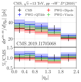
Figure 13: Muon pseudo-rapidity in $pp\to WD^{*}$ events at $\sqrt{s}=13$ TeV, using the selection cuts of the CMS analysis of Ref. CMS:2018dxg , which are implemented in the Rivet analysis CMS_2019_I705068. The experimental data and their combined statistical and systematic errors are drawn in black. The particle-level results obtained interfacing the POWHEG BOX RES with the Herwig7.2 (QTilde, in blue) and the Pythia8.3 showers (Dipole, in red, and Vincia, in green) are also shown together with their scale-uncertainty bands, produced by varying $\mu_{\mathchoice{\displaystyle}{\scriptstyle}{\scriptscriptstyle}{\scriptscriptstyle}\rm F}$ and $\mu_{\mathchoice{\displaystyle}{\scriptstyle}{\scriptscriptstyle}{\scriptscriptstyle}\rm R}$ in the PWG calculation, performing the 7-point scale variations of Eq. (12).

The results of our comparison are illustrated in Fig. 13 for the inclusive $W^{\mp}D^{*}(2010)^{\pm}$ process, on the left panel, for $W^{+}D^{*}(2010)^{-}$, on the middle panel, and for the $W^{-}D^{*}(2010)^{+}$ signature, on the right panel. Among all the showers, Vincia seems to be following the data more closely, slightly underestimating them, in the default Pythia8.3 configuration, while the Herwig7.2 results do instead lead to a larger value of the cross section. We notice that the Dipole shower distributions showed here are very similar to the ones presented in Ref. Bevilacqua:2021ovq , where different PDF sets and tunes were employed. We want however to stress that we use the default tune of the showers, and this distribution is particularly sensitive to the hadronization modelling. For example, the Herwig7.2 hadronization parameters have been tuned in Ref. Bewick:2019rbu using LEP data at the $Z$ mass. Due to the fact that $B$ mesons primarily decay into $D$ ones, the charm hadronization is further affected by its interplay with the bottom hadronization. Thus, a dedicated tune will certainly allow for a better comparison with the data.

5 Conclusions

In this article we have presented the implementation of a NLO + parton-shower generator for massive-charm production in association with a leptonically-decaying $W$ boson in hadron collisions in the POWHEG BOX RES framework. This process is particularly crucial for the determination of the strange-quark content of the proton.

All spin-correlation effects and off-shell contributions in the $W$ decay are properly included, and also non-diagonal elements in the Cabibbo-Kobayashi-Maskawa matrix.

The leading-order and the one-loop matrix elements have been computed analytically, allowing for a very fast and numerically-stable evaluation of the amplitudes.

Using the flexibility of the POWHEG method on the possibility to separate the real-radiation contribution into a finite and a divergent part, that is then exponentiated in the Sudakov form factor, we have implemented different ways to separate the real term and assessed the sensitivity of several kinematic distributions to this extra degree of freedom.

The main source of theoretical uncertainty remains the dependence on the factorization and renormalization scales, of the order of 10% for most kinematic distributions.

Events generated with our code have been interfaced with the Herwig7.2 QTilde shower, as well with the Pythia8.3 default shower and the Vincia one. We have investigated the effect of the parton shower, hadronization and of the underlying-event activity on several kinematic distributions. In particular hadronization corrections turned out to have the highest impact on the differential cross sections.

Particle-level results obtained with the three shower models we have used agree very well with each other, once hadronization corrections and the underlying-event simulation are also included.

Finally we compared our results with the CMS data for the $WD^{*}$ signature, finding good agreement, within the scale-variation bands.

References

- (1) U. Baur, F. Halzen, S. Keller, M. L. Mangano and K. Riesselmann, The Charm content of + 1 jet events as a probe of the strange quark distribution function, Phys. Lett. B 318 (1993) 544–548, [hep-ph/9308370].
- (2) ATLAS collaboration, G. Aad et al., Measurement of the production of a boson in association with a charm quark in collisions at 7 TeV with the ATLAS detector, JHEP 05 (2014) 068, [1402.6263].
- (3) ATLAS collaboration, Measurement of the production of a boson in association with a charmed hadron in collisions at with the ATLAS detector, 2302.00336.
- (4) CMS collaboration, S. Chatrchyan et al., Measurement of Associated W + Charm Production in pp Collisions at = 7 TeV, JHEP 02 (2014) 013, [1310.1138].
- (5) CMS collaboration, A. Tumasyan et al., Measurements of the associated production of a W boson and a charm quark in proton–proton collisions at , Eur. Phys. J. C 82 (2022) 1094, [2112.00895].
- (6) CMS collaboration, A. M. Sirunyan et al., Measurement of associated production of a W boson and a charm quark in proton-proton collisions at 13 TeV, Eur. Phys. J. C 79 (2019) 269, [1811.10021].
- (7) LHCb collaboration, R. Aaij et al., Study of boson production in association with beauty and charm, Phys. Rev. D 92 (2015) 052001, [1505.04051].
- (8) W. T. Giele, S. Keller and E. Laenen, QCD corrections to boson plus heavy quark production at the Tevatron, Phys. Lett. B 372 (1996) 141–149, [hep-ph/9511449].
- (9) W. J. Stirling and E. Vryonidou, Charm production in association with an electroweak gauge boson at the LHC, Phys. Rev. Lett. 109 (2012) 082002, [1203.6781].
- (10) M. Czakon, A. Mitov, M. Pellen and R. Poncelet, NNLO QCD predictions for W+c-jet production at the LHC, JHEP 06 (2021) 100, [2011.01011].
- (11) M. Czakon, A. Mitov, M. Pellen and R. Poncelet, A detailed investigation of W+c-jet at the LHC, JHEP 02 (2023) 241, [2212.00467].
- (12) G. Bevilacqua, M. V. Garzelli, A. Kardos and L. Toth, W+charm production with massive c quarks in PowHel, 2106.11261.
- (13) P. Nason, A New method for combining NLO QCD with shower Monte Carlo algorithms, JHEP 11 (2004) 040, [hep-ph/0409146].
- (14) S. Frixione and B. R. Webber, Matching NLO QCD computations and parton shower simulations, JHEP 06 (2002) 029, [hep-ph/0204244].
- (15) J. Alwall, R. Frederix, S. Frixione, V. Hirschi, F. Maltoni, O. Mattelaer et al., The automated computation of tree-level and next-to-leading order differential cross sections, and their matching to parton shower simulations, JHEP 07 (2014) 079, [1405.0301].
- (16) P. Nason, C. Oleari, M. Rocco and M. Zaro, An interface between the POWHEG BOX and MadGraph5aMC@NLO, Eur. Phys. J. C 80 (2020) 985, [2008.06364].
- (17) S. Frixione, P. Nason and C. Oleari, Matching NLO QCD computations with Parton Shower simulations: the POWHEG method, JHEP 11 (2007) 070, [0709.2092].
- (18) S. Alioli, P. Nason, C. Oleari and E. Re, A general framework for implementing NLO calculations in shower Monte Carlo programs: the POWHEG BOX, JHEP 06 (2010) 043, [1002.2581].
- (19) T. Ježo and P. Nason, On the Treatment of Resonances in Next-to-Leading Order Calculations Matched to a Parton Shower, JHEP 12 (2015) 065, [1509.09071].
- (20) L. Barze, G. Montagna, P. Nason, O. Nicrosini and F. Piccinini, Implementation of electroweak corrections in the POWHEG BOX: single W production, JHEP 04 (2012) 037, [1202.0465].
- (21) J. Mazzitelli, P. F. Monni, P. Nason, E. Re, M. Wiesemann and G. Zanderighi, Next-to-Next-to-Leading Order Event Generation for Top-Quark Pair Production, Phys. Rev. Lett. 127 (2021) 062001, [2012.14267].
- (22) J. Mazzitelli, P. F. Monni, P. Nason, E. Re, M. Wiesemann and G. Zanderighi, Top-pair production at the LHC with MINNLOPS, JHEP 04 (2022) 079, [2112.12135].
- (23) S. Zanoli, M. Chiesa, E. Re, M. Wiesemann and G. Zanderighi, Next-to-next-to-leading order event generation for VH production with H → decay, JHEP 07 (2022) 008, [2112.04168].
- (24) A. Gavardi, C. Oleari and E. Re, NNLO+PS Monte Carlo simulation of photon pair production with MiNNLOPS, JHEP 09 (2022) 061, [2204.12602].
- (25) P. F. Monni, P. Nason, E. Re, M. Wiesemann and G. Zanderighi, MiNNLOPS: a new method to match NNLO QCD to parton showers, JHEP 05 (2020) 143, [1908.06987].
- (26) P. F. Monni, E. Re and M. Wiesemann, MiNNLO: optimizing hadronic processes, Eur. Phys. J. C 80 (2020) 1075, [2006.04133].
- (27) G. Cullen et al., GS-2.0: a tool for automated one-loop calculations within the Standard Model and beyond, Eur. Phys. J. C 74 (2014) 3001, [1404.7096].
- (28) G. Cullen, N. Greiner, G. Heinrich, G. Luisoni, P. Mastrolia, G. Ossola et al., Automated One-Loop Calculations with GoSam, Eur. Phys. J. C 72 (2012) 1889, [1111.2034].
- (29) J. Alwall, P. Demin, S. de Visscher, R. Frederix, M. Herquet, F. Maltoni et al., MadGraph/MadEvent v4: The New Web Generation, JHEP 09 (2007) 028, [0706.2334].
- (30) J. M. Campbell, R. K. Ellis, R. Frederix, P. Nason, C. Oleari and C. Williams, NLO Higgs Boson Production Plus One and Two Jets Using the POWHEG BOX, MadGraph4 and MCFM, JHEP 07 (2012) 092, [1202.5475].
- (31) J. C. Collins, F. Wilczek and A. Zee, Low-Energy Manifestations of Heavy Particles: Application to the Neutral Current, Phys. Rev. D 18 (1978) 242.
- (32) T. Appelquist and J. Carazzone, Infrared Singularities and Massive Fields, Phys. Rev. D 11 (1975) 2856.
- (33) M. Cacciari, M. Greco and P. Nason, The spectrum in heavy flavor hadroproduction, JHEP 05 (1998) 007, [hep-ph/9803400].
- (34) G. Luisoni, C. Oleari and F. Tramontano, production at NLO with POWHEG+MiNLO, JHEP 04 (2015) 161, [1502.01213].
- (35) A. Buckley, J. Ferrando, S. Lloyd, K. Nordström, B. Page, M. Rüfenacht et al., LHAPDF6: parton density access in the LHC precision era, Eur. Phys. J. C 75 (2015) 132, [1412.7420].
- (36) NNPDF collaboration, R. D. Ball et al., Parton distributions from high-precision collider data, Eur. Phys. J. C 77 (2017) 663, [1706.00428].
- (37) J. Campbell and T. Neumann, Precision Phenomenology with MCFM, JHEP 12 (2019) 034, [1909.09117].
- (38) J. M. Campbell, R. K. Ellis and W. T. Giele, A Multi-Threaded Version of MCFM, Eur. Phys. J. C 75 (2015) 246, [1503.06182].
- (39) J. Bellm, G. Nail, S. Plätzer, P. Schichtel and A. Siódmok, Parton Shower Uncertainties with Herwig 7: Benchmarks at Leading Order, Eur. Phys. J. C 76 (2016) 665, [1605.01338].
- (40) M. Cacciari, G. P. Salam and G. Soyez, FastJet User Manual, Eur. Phys. J. C 72 (2012) 1896, [1111.6097].
- (41) M. Cacciari, G. P. Salam and G. Soyez, The anti- jet clustering algorithm, JHEP 04 (2008) 063, [0802.1189].
- (42) M. Bahr et al., Herwig++ Physics and Manual, Eur. Phys. J. C 58 (2008) 639–707, [0803.0883].
- (43) J. Bellm et al., Herwig 7.2 release note, Eur. Phys. J. C 80 (2020) 452, [1912.06509].
- (44) T. Sjostrand, S. Mrenna and P. Z. Skands, PYTHIA 6.4 Physics and Manual, JHEP 05 (2006) 026, [hep-ph/0603175].
- (45) T. Sjöstrand, S. Ask, J. R. Christiansen, R. Corke, N. Desai, P. Ilten et al., An introduction to PYTHIA 8.2, Comput. Phys. Commun. 191 (2015) 159–177, [1410.3012].
- (46) B. Cabouat and T. Sjöstrand, Some Dipole Shower Studies, Eur. Phys. J. C 78 (2018) 226, [1710.00391].
- (47) H. Brooks, C. T. Preuss and P. Skands, Sector Showers for Hadron Collisions, JHEP 07 (2020) 032, [2003.00702].
- (48) P. Skands and R. Verheyen, Multipole photon radiation in the Vincia parton shower, Phys. Lett. B 811 (2020) 135878, [2002.04939].
- (49) S. Catani, B. R. Webber and G. Marchesini, QCD coherent branching and semiinclusive processes at large x, Nucl. Phys. B 349 (1991) 635–654.
- (50) C. Bierlich et al., Robust Independent Validation of Experiment and Theory: Rivet version 3, SciPost Phys. 8 (2020) 026, [1912.05451].
- (51) G. Bewick, S. Ferrario Ravasio, P. Richardson and M. H. Seymour, Logarithmic accuracy of angular-ordered parton showers, JHEP 04 (2020) 019, [1904.11866].