Robust Formulation of Wick’s theorem for Computing Matrix Elements Between Hartree–Fock–Bogoliubov Wavefunctions
Abstract
Numerical difficulties associated with computing matrix elements of operators between Hartree–Fock–Bogoliubov (HFB) wavefunctions have plagued the development of HFB-based many-body theories for decades. The problem arises from divisions by zero in the standard formulation of the nonorthogonal Wick’s theorem in the limit of vanishing HFB overlap. In this paper, we present a robust formulation of Wick’s theorem that stays well-behaved regardless of whether the HFB states are orthogonal or not. This new formulation ensures cancellation between the zeros of the overlap and the poles of the Pfaffian, which appears naturally in fermionic systems. Our formula explicitly eliminates self-interaction, which otherwise causes additional numerical challenges. A computationally efficient version of our formalism enables robust symmetry-projected HFB calculations with the same computational cost as mean-field theories. Moreover, we avoid potentially diverging normalization factors by introducing a robust normalization procedure. The resulting formalism treats even and odd number of particles on equal footing and reduces to Hartree–Fock as a natural limit. As proof of concept, we present a numerically stable and accurate solution to a Jordan–Wigner-transformed Hamiltonian, whose singularities motivated the present work. Our robust formulation of Wick’s theorem is a most promising development for methods using quasiparticle vacuum states.
I Introduction
The Hartree–Fock–Bogoliubov (HFB) wavefunction is a fermionic mean-field ansatz allowing particle number symmetry breaking.[1, 2] It encompasses the Hartree–Fock (HF) wavefunction in the same sense that spin-unrestricted HF (UHF) reduces to spin-restricted HF (RHF) without spin symmetry breaking. HFB-based methods are not as conventional in quantum chemistry as in nuclear structure theory. This is a consequence of repulsive electronic interactions in the former, which results in number symmetry not breaking spontaneously in mean-field.[3]
Nevertheless, the emergence of variation-after-projection approaches to symmetry breaking and restoration [4, 5, 6, 7] has sparked growing interest in HFB and related anzätze in electronic structure theory. [6, 8, 9, 10, 11, 12, 13, 14, 15, 16, 17, 18, 19, 20, 21, 22, 23, 24, 25, 26] Methods based on symmetry-projected HFB (PHFB) are particularly promising for describing strongly correlated systems, where traditional HF-based methods fail.[6, 27, 28, 29]
Essential for the implementation of PHFB-based methods are matrix elements of many-body operators between nonorthogonal HFB states. Indeed, the PHFB formalism can be considered a general form of nonorthogonal configuration interaction (NOCI).[30, 31] The computation of relevant matrix elements relies on the generalized Wick’s theorem with respect to nonorthogonal HFB states, also known as the nonorthogonal Wick’s theorem.[32, 33]
However, when the overlap between right and left HFB states vanishes, the standard formula in the nonorthogonal Wick’s theorem becomes numerically ill-conditioned, and eventually ill-defined, causing large round-off errors. This problem occurs in PHFB calculations[34, 35] and is exacerbated by self-interaction[36, 37] if exchange- or pairing-type contractions are neglected, e.g., within the context of nuclear density functional theory. [38, 39, 37, 40]
Our recent work mapping spin systems to fermions using the Jordan–Wigner transformation[41, 42] is another example where orthogonal HFB wavefunctions arise and lead to large numerical errors. This happens when fermionic on-site occupations are equal to , which is frequently encountered in frustrated phases of transformed spin systems.
The main objective of this paper is to demonstrate that with proper algorithmic design, the nonorthogonal Wick’s theorem can be extended to the orthogonal limit, resulting in accurate and efficient computation of matrix elements between arbitrary HFB states. Related algorithms have been discussed for HF-based NOCI,[43, 44, 45, 46] and our formalism reduces to them in that limit. Remedies for the numerical problems encountered in the HFB case have been proposed for specific applications[34, 35] or under certain restrictions. [47, 48] However, a universal, low-scaling formula for robust computation of matrix elements between HFB states, as the one presented here, was lacking.
II Nonorthogonal Wick’s Theorem
We define unnormalized HFB wavefunctions or quasiparticle vacuum states, and , as
| (1) |
for , where denotes the physical vacuum, and is the dimension of the one-particle (spin-orbital) basis. The Bogoliubov quasiparticle annihilation operators are related to the fermionic particle operators and through a unitary canonical transformation known as the Bogoliubov transformation:
| (2) |
To ensure nonvanishing , we assume that is non-singular, i.e., all of the canonical orbitals of obtained from the Bloch–Messiah decomposition[49] of and (vide infra) are at least infinitesimally occupied. We will eliminate this assumption and address the normalization of in Sec. V.
The nonorthogonal Wick’s theorem can be concisely stated using the Pfaffian as follows:[50] For , a matrix element of a -body operator is expressed as
| (3) |
where is a set of arbitrary fermionic operators, and is a antisymmetric matrix whose strict upper triangular part is defined by contractions of the form
| (4) |
for . The Pfaffian automatically generates all possible full contractions of the fermionic operators with the correct signs, reflecting the fermionic anticommutation relations. For example, Eq. (3) reduces to the conventional statement of the nonorthogonal Wick’s theorem [32, 33, 1, 2] for the two-particle reduced transition matrix (-RTM), [51, 52, 53] or second-order transition density matrix:
| (5) |
where
| (6) |
and we follow the convention that each crossing between contraction lines introduces a minus sign, which is implied by the properties of the Pfaffian. In general, we can write as a quasiparticle
| (7) |
where and are matrices. Note that for , and may come from different Bogoliubov transformations, hence the superscript in our notation.
We see from Eq. (4) that the nonorthogonal Wick’s theorem becomes ill-defined when . In this case, we may fall back to the original Wick’s theorem with respect to the physical vacuum. [54, 55, 56] We have[57]
| (8a) | ||||
| (8b) | ||||
where is a antisymmetric matrix defined by
| (9) |
for . Compared with Eq. (3), Eq. (8) is always well-defined, but the Pfaffian of a much larger matrix needs to be evaluated, greatly increasing the computational cost.
In the following, we sketch a proof of the nonorthogonal Wick’s theorem stated in Eq. (3), introducing our notation along the way. Unlike the proof by induction presented in Ref. 50, our proof follows a more direct approach inspired by Ref. 58. We start by rewriting Eq. (8) using the properties of the Pfaffian:
| (10) |
where
| (11) |
| (12) |
and
| (13) |
When , the antisymmetric matrix is non-singular since[57]
| (14) |
We therefore have the following Pfaffian identity
| (15) |
where denotes the Schur complement of the block of the supermatrix , i.e.,
| (16) |
On the other hand, as shown in detail in the supplementary material, we find
| (17) |
and it follows that
| (18) |
Inserting Eqs. (14) and (18) into Eqs. (10) and (15) completes the proof.
Without loss of generality, we hereafter assume that are particle operators in normal order with respect to the physical vacuum. Thus, we have and
| (19) |
These particular matrix elements contain those that arise in the -particle or th-order reduced transition matrix (-RTM), [51, 52, 53]
| (20) |
Eq. (19) is reminiscent of Löwdin’s formula for -RTM between HF wavefunctions, [59] for which singular value decomposition (SVD) can be used to extract the zeros and poles in order to evaluate the zero-overlap limit. [43, 44, 45, 46] We show in the next section that this idea can be generalized to the HFB case.
III Robust Wick’s Theorem
The antisymmetric matrix can be written in canonical form, [60, 61]
| (21) |
where is unitary and
| (22) |
The elements of the vector are nonnegative and they reduce to the singular values of the overlap matrix in the HF case, as shown in the supplementary material. Moreover, it follows from Eq. (14) that
| (23) |
where is a complex phase factor. We observe that the poles of in Eq. (19) get cancelled out by the zeros of the overlap, hinting at a more general and robust formula for computing matrix elements.
Define
| (24) |
where
| (25a) | ||||
| (25b) | ||||
| (25c) | ||||
and
| (26) |
It is straightforward to show
| (27) |
We now propose a robust formulation of Wick’s theorem for computing matrix elements between HFB wavefunctions:
| (28) |
with
| (29) |
| (30) |
where denotes tensor product, enumerates permutations in the symmetric group , and is the signature of . Eq. (30) defines a special case of the hyper-Pfaffian,[62, 63] denoted by , which generalizes the Pfaffian to tensors. For the general definition of the hyper-Pfaffian, we refer the reader to the supplementary material.
The proof of the theorem is presented in the supplementary material. We emphasize that the formula in Eq. (28) remains well-behaved with vanishing because all potential divisions by zero have been prevented by construction. Specifically, all factors are cancelled out by the factors of in Eq. (23), while all terms involving , , etc., drop out due to the cancellation of self-interaction. The latter is guaranteed by the properties of the Pfaffian and is further enforced numerically by setting to zero when its indices are not distinct. From the definition of , we can also see that the matrix element vanishes if the number of zero elements in exceeds , consistent with the Slater–Condon rules between HF wavefunctions; [64, 65, 51] see the next section for generalization to the HFB case.
In practical calculations, we do not need to explicitly evaluate the hyper-Pfaffian for each individual matrix element. Instead, Eq. (28) generates expressions of high-order RTMs in terms of the modified contractions defined in Eq. (25). As an example, the robust Wick’s theorem implies the following expression of the -RTM:
| (31) |
where we have used . Computing the full -RTM using Eq. (31) scales as . In practice, however, we never construct the full -RTM. To compute the matrix element of a two-body operator, we can directly contract its parameters (e.g., two-electron integrals) with the factorized form of the -RTM in Eq. (31). For example, the tensor contraction between the two-electron integrals and the -RTM should scale as to after exploiting locality using standard techniques. [66, 67, 68]
IV Low-Scaling Version
We may further reduce the scaling by enforcing the cancellation only of the smallest elements in . We partition into singular () and regular () parts according to
| (32) |
where . The value of should be so chosen that is well-conditioned while the size of is small. Similarly, we define , , and as the regular parts of , , and , respectively. By the properties of the hyper-Pfaffian, we can now establish a low-scaling robust Wick’s theorem, which states that
| (33) |
where
| (34a) | |||
| (34b) |
and we have used
| (35) |
If is empty, Eq. (33) reduces to the nonorthogonal Wick’s theorem in Eq. (3).
Applying the low-scaling robust Wick’s theorem to -RTM, we have
| (36) |
and similarly for and . Each term in the above expression stays factorized, facilitating low-scaling tensor contractions with the electron integrals. Besides, the indices , now only run over a small subset of elements. As a result, the computational cost of the matrix element of a two-body operator scales the same as that of HF, i.e., to , albeit with a larger prefactor. For -RTM with , the reduction of computational scaling from Eq. (28) to Eq. (33) is even more significant.
We can now generalize the Slater–Condon rules to the HFB case using the low-scaling robust Wick’s theorem. Let be the number of elements that are strictly zero. Loosely speaking, equals the smallest number of levels we need to block in both and in order to make them nonorthogonal. The blocking should be done in a biorthogonal basis that simultaneously brings both and to the canonical form of the Bardeen–Cooper–Schrieffer (BCS) ansatz. [69, 47, 48] This biorthogonal basis is generally nonunitary and does not always exist as noted in Ref. 48. It is readily seen from Eq. (33) that the term vanishes for , the and terms vanish for , and so forth. These results resemble the generalized Slater–Condon rules for HF matrix elements, [70, 44, 46] in which case corresponds to the smallest number of biorthogonal occupied orbital pairs that need to be emptied in order to make the HF wavefunctions nonorthogonal. Here the biorthogonalization is guaranteed by Löwdin pairing and realized by SVD. [71, 72, 73] We should point out that, as opposed to the generalized Slater–Condon rules, our Eq. (33) also ensures numerical stability when some elements of are small but not strictly zero.
V Robust Normalization
So far we have considered unnormalized HFB wavefunctions for as defined in Eq. (1). The corresponding normalized HFB wavefunction is[57]
| (37) |
where and come from the Bloch–Messiah decomposition,[49]
| (38) |
with and being unitary and
| (39a) | ||||
| (39b) | ||||
Here denotes the identity matrix, and denotes the -component of the Pauli matrices; are positive real numbers and satisfy . Note that we use an unconventional definition of in Eq. (39), which is physically inconsequential but will ease the notation in what follows. The Bloch–Messiah decomposition implies that, in the canonical basis of with orbital coefficients , we have fully occupied core orbitals, paired fractionally occupied orbitals, and unoccupied or virtual orbitals, with .
The normalization factor in Eq. (37) is generally unbounded, which may introduce additional numerical challenges. To overcome this problem, we define a set of unnormalized quasiparticles by an unnormalized Bogoliubov transformation:
| (40) |
for , with
| (41) |
where is built from the first columns of as suggested in Ref. 74, and
| (42a) | ||||
| (42b) | ||||
It is readily shown that the normalized HFB wavefunction is the vacuum state of these unnormalized quasiparticles, i.e.,
| (43) |
Furthermore,
| (44a) | ||||
| (44b) | ||||
whose elements are bounded by in absolute value even though is generally unbounded. Therefore, we no longer have to deal with the problematic normalization factor in Eq. (37) as long as we compute the overlap between normalized HFB wavefunctions using
| (45) |
This procedure for computing the overlap is similar to the one proposed in Ref. 75; however, we emphasize that our formalism, as opposed to those in Refs. 57 and 75, treats even- and odd-particle systems on the same footing, since the number of core orbitals from the Bloch–Messiah decomposition is not restricted to be even. Other formalisms for equally accounting for even and odd number parities have been suggested, without addressing the numerical pitfalls of the unbounded normalization factors. [76, 77, 78]
More importantly, our robust normalization procedure for computing the overlap is compatible with the robust Wick’s theorem and its low-scaling version. Namely, Eqs. (28) and (33) remain valid for the -RTM between the normalized and after formally replacing with , or equivalently replacing with and with
| (46) |
This correspondence is apparent from Eq. (19), whose derivation does not rely on the normalization of the Bogoliubov transformations.
Finally, we note in passing that, when , reduces to a HF wavefunction, so the robust Wick’s theorem and its low-scaling variant can also be used to compute HF reduced transition matrices (see the supplementary material). All pairing-type contractions are removed in this case due to vanishing and .
VI Numerical Example
We here present a prototypical example to demonstrate the power of our proposed robust Wick’s theorem. The Heisenberg XXZ Hamiltonian can be treated as a fermionic system after Jordan–Wigner (JW) transformation. The claim to fame of this mapping is that in 1D at , a maximally degenerate point, the transformed Hamiltonian becomes a free fermion system readily solvable by mean-field HF theory. Here, is the anisotropy parameter. We refer the reader to Ref. 42 for details of the transformed Hamiltonian. For , number symmetry breaks spontaneously, necessitating HFB solutions. Matrix elements of the form
| (47) |
need to be computed for , where the JW string
| (48) |
is a Thouless rotation acting on with . The overlap
| (49) |
vanishes when for , a situation we observe across the critical region of the 1D phase diagram. On the other hand, because XXZ possess only nearest neighbor interactions, one can avoid dealing with JW strings all together and analytically show that
| (50) |
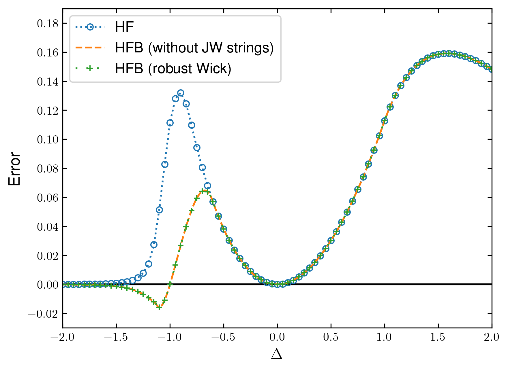
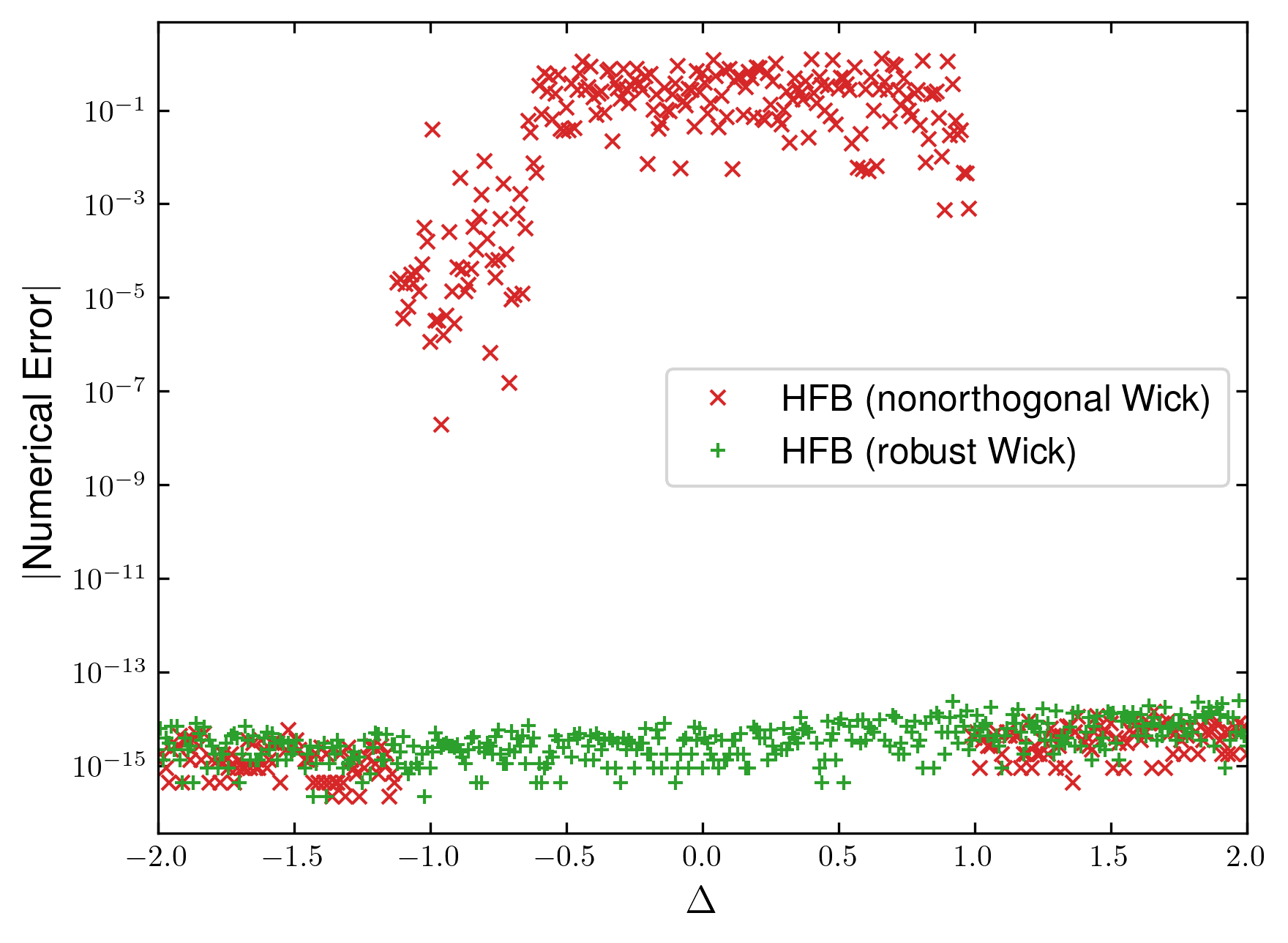
The right hand side of Eq. (50) is numerically well-posed because , after applying the normalization procedure in Sec. V. Therefore, we have two analytically equivalent forms of evaluating the same matrix elements. Comparing numerical results from Eq. (47), which generates orthogonal HFB states, and Equation(50), we can measure the round-off errors due to vanishing and verify that our robust Wick’s theorem eliminates them.
Consider a JW-transformed 8-site XXZ chain with open boundary conditions. We constrain , which corresponds to . We find that for all with . We observe equal site occupations ( in the original spin representation) within this range of values, consistent with our previous calculations using a spin antisymmetrized geminal power ansatz.[79] As shown in Fig. 1, the HFB energies obtained from Eq. (47) using the nonorthogonal Wick’s theorem indeed suffer from severe numerical error in this regime. In contrast, the robust Wick’s theorem, yields energies on top of the exact results computed without JW strings using Eq. (50).
VII Concluding Remarks
In quantum mechanical calculations with nonorthogonal basis, negligible overlaps do not necessarily imply negligible interactions, as one might erroneously infer from the nonorthogonal Wick’s theorem in Eq. (3), where the matrix element is proportional to the overlap . The fallacy originates from the fact that Eq. (3) is ill-defined when , as shown by our formal and numerical analyses. Accurate computation of the matrix element requires evaluating the limit of Eq. (3) as , which is always well-defined and can be nonzero in general.
The idea of taking the limit before numerical evaluation is a recurring theme of this paper. It underlies how we resolve the two major limitations of the standard formulation of the nonorthogonal Wick’s theorem:
-
•
First, when vanishes, the Pfaffian in Eq. (3) develop poles even after self-interaction is eliminated. We have addressed this issue in Sec. III by cancelling these poles with the zeros of the overlap. The resulting robust formulation of Wick’s theorem is universally applicable and numerically stable for computing matrix elements between HFB wavefunctions. And it remains amenable to efficient implementation as shown in Sec. IV.
-
•
Second, the normalization factors for and may become divergingly large. We have addressed this issue in Sec. V by introducing a robust normalization procedure. This is achieved by formally viewing normalized HFB wavefunctions as vacuum states of unnormalized quasiparticles. Although the coefficients defining these unnormalized quasiparticles are unbounded in general, the and matrices entering the final expressions for the matrix elements remain bounded.
We expect the present work to have a broad impact in quantum many-body theories, facilitating future developments of methods based on quasiparticle vacuum states. One promising area of application is HFB-based NOCI or generator coordinate method (GCM) in general. [30, 31] Not only do these methods recover important ground-state correlations, [6, 12] but they are also expected to be suitable for describing excited states, particularly those of charge transfer or double excitation character. [80, 81, 82] Moreover, PHFB is closely related to geminal theories. [6, 83, 84, 85] Our formalism can be applied to compute matrix elements between number-projected HFB (NHFB) or antisymmetrized geminal power (AGP) states, especially for ones that do not share the same set of canonical orbitals. Another potential application is correlated methods using HFB or PHFB as the reference state. [86, 87, 88, 18, 24] Reduced transition matrices encountered in these methods are typically of high order, for which the low-scaling version of our robust Wick’s theorem becomes useful.
Supplementary Material
The supplementary material contains definitions of the Pfaffian and hyper-Pfaffian along with detailed proofs of equations and theorems in the main text. We also show therein how our robust formulation of Wick’s theorem reduces to the RTM expressions in Ref. 43 in the Hartree–Fock limit.
Acknowledgements.
This work was supported by the U.S. National Science Foundation under Grant No. CHE-2153820. G.E.S. is a Welch Foundation Chair (Grant No. C-0036). G.P.C. thanks Thomas M. Henderson for helpful discussions and useful comments.References
- Ring and Schuck [1980] P. Ring and P. Schuck, The nuclear many-body problem (Springer-Verlag, Berlin Heidelberg, 1980).
- Blaizot and Ripka [1986] J.-P. Blaizot and G. Ripka, Quantum theory of finite systems (MIT Press, Cambridge, Mass., 1986).
- Lieb [1981] E. H. Lieb, “Variational principle for many-fermion systems,” Phys. Rev. Lett 46, 457–459 (1981).
- Sheikh and Ring [2000] J. A. Sheikh and P. Ring, “Symmetry-projected Hartree–Fock–Bogoliubov equations,” Nucl. Phys. A 665, 71–91 (2000).
- Schmid [2004] K. W. Schmid, “On the use of general symmetry-projected Hartree–Fock–Bogoliubov configurations in variational approaches to the nuclear many-body problem,” Prog. Part. Nucl. Phys. 52, 565–633 (2004).
- Scuseria et al. [2011] G. E. Scuseria, C. A. Jiménez-Hoyos, T. M. Henderson, K. Samanta, and J. K. Ellis, “Projected quasiparticle theory for molecular electronic structure,” J. Chem. Phys. 135, 124108 (2011).
- Sheikh et al. [2021] J. A. Sheikh, J. Dobaczewski, P. Ring, L. M. Robledo, and C. Yannouleas, “Symmetry restoration in mean-field approaches,” J. Phys. G: Nucl. Part. Phys. 48, 123001 (2021).
- Naftchi-Ardebili, Hau, and Mazziotti [2011] K. Naftchi-Ardebili, N. W. Hau, and D. A. Mazziotti, “Rank restriction for the variational calculation of two-electron reduced density matrices of many-electron atoms and molecules,” Phys. Rev. A 84, 052506 (2011).
- Neuscamman [2012] E. Neuscamman, “Size consistency error in the antisymmetric geminal power wave function can be completely removed,” Phys. Rev. Lett. 109, 203001 (2012).
- Neuscamman [2013] E. Neuscamman, “The Jastrow antisymmetric geminal power in Hilbert space: Theory, benchmarking, and application to a novel transition state,” J. Chem. Phys. 139, 194105 (2013).
- Jiménez-Hoyos, Rodríguez-Guzmán, and Scuseria [2012] C. A. Jiménez-Hoyos, R. Rodríguez-Guzmán, and G. E. Scuseria, “-electron Slater determinants from nonunitary canonical transformations of fermion operators,” Phys. Rev. A 86, 052102 (2012).
- Uemura, Kasamatsu, and Sugino [2015] W. Uemura, S. Kasamatsu, and O. Sugino, “Configuration interaction with antisymmetrized geminal powers,” Phys. Rev. A 91, 062504 (2015).
- Tsuchimochi, Welborn, and Van Voorhis [2015] T. Tsuchimochi, M. Welborn, and T. Van Voorhis, “Density matrix embedding in an antisymmetrized geminal power bath,” J. Chem. Phys. 143, 024107 (2015).
- Degroote et al. [2016] M. Degroote, T. M. Henderson, J. Zhao, J. Dukelsky, and G. E. Scuseria, “Polynomial similarity transformation theory: A smooth interpolation between coupled cluster doubles and projected BCS applied to the reduced BCS Hamiltonian,” Phys. Rev. B 93, 125124 (2016).
- Shi and Zhang [2017] H. Shi and S. Zhang, “Many-body computations by stochastic sampling in Hartree–Fock–Bogoliubov space,” Phys. Rev. B 95, 045144 (2017).
- Mahajan and Sharma [2019] A. Mahajan and S. Sharma, “Symmetry-projected Jastrow mean-field wave function in variational Monte Carlo,” J. Phys. Chem. A 123, 3911–3921 (2019).
- Khamoshi, Henderson, and Scuseria [2019] A. Khamoshi, T. M. Henderson, and G. E. Scuseria, “Efficient evaluation of AGP reduced density matrices,” J. Chem. Phys. 151, 184103 (2019).
- M. Henderson and E. Scuseria [2020] T. M. Henderson and G. E. Scuseria, “Correlating the antisymmetrized geminal power wave function,” J. Chem. Phys. 153, 084111 (2020).
- Dutta, Henderson, and Scuseria [2020] R. Dutta, T. M. Henderson, and G. E. Scuseria, “Geminal replacement models based on AGP,” J. Chem. Theory Comput. 16, 6358–6367 (2020).
- Larsson, Jiménez-Hoyos, and Chan [2020] H. R. Larsson, C. A. Jiménez-Hoyos, and G. K.-L. Chan, “Minimal matrix product states and generalizations of mean-field and geminal wave functions,” J. Chem. Theory Comput. 16, 5057–5066 (2020).
- Johnson et al. [2020] P. A. Johnson, C.-É. Fecteau, F. Berthiaume, S. Cloutier, L. Carrier, M. Gratton, P. Bultinck, S. De Baerdemacker, D. Van Neck, P. Limacher, and P. W. Ayers, “Richardson–Gaudin mean-field for strong correlation in quantum chemistry,” J. Chem. Phys. 153, 104110 (2020).
- Khamoshi, Evangelista, and Scuseria [2021] A. Khamoshi, F. A. Evangelista, and G. E. Scuseria, “Correlating AGP on a quantum computer,” Quantum Sci. Technol. 6, 014004 (2021).
- Lin and Wu [2021] L. Lin and X. Wu, “Numerical solution of large scale Hartree–Fock–Bogoliubov equations,” ESAIM: M2AN 55, 763–787 (2021).
- Khamoshi et al. [2021] A. Khamoshi, G. P. Chen, T. M. Henderson, and G. E. Scuseria, “Exploring non-linear correlators on AGP,” J. Chem. Phys. 154, 074113 (2021).
- Dutta et al. [2021] R. Dutta, G. P. Chen, T. M. Henderson, and G. E. Scuseria, “Construction of linearly independent non-orthogonal AGP states,” J. Chem. Phys. 154, 114112 (2021).
- Khamoshi et al. [2023] A. Khamoshi, G. P. Chen, F. A. Evangelista, and G. E. Scuseria, “AGP-based unitary coupled cluster theory for quantum computers,” Quantum Sci. Technol. 8, 015006 (2023).
- Yang [1962] C. N. Yang, “Concept of off-diagonal long-range order and the quantum phases of liquid He and of superconductors,” Rev. Mod. Phys. 34, 694–704 (1962).
- Coleman [1965] A. J. Coleman, “Structure of fermion density matrices. II. Antisymmetrized geminal powers,” J. Math. Phys. 6, 1425–1431 (1965).
- Sager and Mazziotti [2022] L. M. Sager and D. A. Mazziotti, “Cooper-pair condensates with nonclassical long-range order on quantum devices,” Phys. Rev. Research 4, 013003 (2022).
- Hill and Wheeler [1953] D. L. Hill and J. A. Wheeler, “Nuclear constitution and the interpretation of fission phenomena,” Phys. Rev. 89, 1102–1145 (1953).
- Peierls and Yoccoz [1957] R. E. Peierls and J. Yoccoz, “The collective model of nuclear motion,” Proc. Phys. Soc. A 70, 381 (1957).
- Onishi and Yoshida [1966] N. Onishi and S. Yoshida, “Generator coordinate method applied to nuclei in the transition region,” Nucl. Phys. 80, 367–376 (1966).
- Balian and Brezin [1969] R. Balian and E. Brezin, “Nonunitary Bogoliubov transformations and extension of Wick’s theorem,” Nuovo Cimento B 64, 37 (1969).
- Tajima et al. [1992] N. Tajima, H. Flocard, P. Bonche, J. Dobaczewski, and P.-H. Heenen, “Generator coordinate kernels between zero- and two-quasiparticle BCS states,” Nucl. Phys. A 542, 355–367 (1992).
- Anguiano, Egido, and Robledo [2001] M. Anguiano, J. L. Egido, and L. M. Robledo, “Particle number projection with effective forces,” Nucl. Phys. A 696, 467–493 (2001).
- Perdew and Zunger [1981] J. P. Perdew and A. Zunger, “Self-interaction correction to density-functional approximations for many-electron systems,” Phys. Rev. B 23, 5048–5079 (1981).
- Bender, Duguet, and Lacroix [2009] M. Bender, T. Duguet, and D. Lacroix, “Particle-number restoration within the energy density functional formalism,” Phys. Rev. C 79, 044319 (2009).
- Dobaczewski et al. [2007] J. Dobaczewski, M. V. Stoitsov, W. Nazarewicz, and P.-G. Reinhard, “Particle-number projection and the density functional theory,” Phys. Rev. C 76, 054315 (2007).
- Lacroix, Duguet, and Bender [2009] D. Lacroix, T. Duguet, and M. Bender, “Configuration mixing within the energy density functional formalism: Removing spurious contributions from nondiagonal energy kernels,” Phys. Rev. C 79, 044318 (2009).
- Duguet et al. [2009] T. Duguet, M. Bender, K. Bennaceur, D. Lacroix, and T. Lesinski, “Particle-number restoration within the energy density functional formalism: Nonviability of terms depending on noninteger powers of the density matrices,” Phys. Rev. C 79, 044320 (2009).
- Jordan and Wigner [1928] P. Jordan and E. Wigner, “Über das paulische äquivalenzverbot,” Z. Phys. 47, 631–651 (1928).
- Henderson, Chen, and Scuseria [2022] T. M. Henderson, G. P. Chen, and G. E. Scuseria, “Strong–weak duality via Jordan–Wigner transformation: Using fermionic methods for strongly correlated spin systems,” J. Chem. Phys. 157, 194114 (2022).
- Koch and Dalgaard [1993] H. Koch and E. Dalgaard, “Linear superposition of optimized non-orthogonal slater determinants for singlet states,” Chem. Phys. Lett. 212, 193–200 (1993).
- J. W. Thom and Head-Gordon [2009] A. J. W. Thom and M. Head-Gordon, “Hartree–Fock solutions as a quasidiabatic basis for nonorthogonal configuration interaction,” J. Chem. Phys. 131, 124113 (2009).
- Rodriguez-Laguna, Robledo, and Dukelsky [2020] J. Rodriguez-Laguna, L. M. Robledo, and J. Dukelsky, “Efficient computation of matrix elements of generic slater determinants,” Phys. Rev. A 101, 012105 (2020).
- Burton [2021] H. G. A. Burton, “Generalized nonorthogonal matrix elements: Unifying Wick’s theorem and the Slater–Condon rules,” J. Chem. Phys. 154, 144109 (2021).
- Dönau [1998] F. Dönau, “Canonical form of transition matrix elements,” Phys. Rev. C 58, 872–877 (1998).
- Dobaczewski [2000] J. Dobaczewski, “Generalization of the Bloch–Messiah–Zumino theorem,” Phys. Rev. C 62, 017301 (2000).
- Bloch and Messiah [1962] C. Bloch and A. Messiah, “The canonical form of an antisymmetric tensor and its application to the theory of superconductivity,” Nucl. Phys. 39, 95–106 (1962).
- Hu, Gao, and Chen [2014] Q.-L. Hu, Z.-C. Gao, and Y. S. Chen, “Matrix elements of one-body and two-body operators between arbitrary HFB multi-quasiparticle states,” Phys. Lett. B 734, 162–166 (2014).
- Löwdin [1955] P.-O. Löwdin, “Quantum theory of many-particle systems. I. Physical interpretations by means of density matrices, natural spin-orbitals, and convergence problems in the method of configurational interaction,” Phys. Rev. 97, 1474–1489 (1955).
- McWeeny [1960] R. McWeeny, “Some recent advances in density matrix theory,” Rev. Mod. Phys. 32, 335–369 (1960).
- Mazziotti [1999] D. A. Mazziotti, “Comparison of contracted Schrödinger and coupled-cluster theories,” Phys. Rev. A 60, 4396–4408 (1999).
- Wick [1950] G. C. Wick, “The evaluation of the collision matrix,” Phys. Rev. 80, 268–272 (1950).
- Gaudin [1960] M. Gaudin, “Une démonstration simplifiée du théorème de Wick en mécanique statistique,” Nucl. Phys. 15, 89–91 (1960).
- Lieb [1968] E. H. Lieb, “A theorem on Pfaffians,” J. Comb. Theory 5, 313–319 (1968).
- Bertsch and Robledo [2012] G. F. Bertsch and L. M. Robledo, “Symmetry restoration in Hartree–Fock–Bogoliubov based theories,” Phys. Rev. Lett. 108, 042505 (2012).
- Mizusaki and Oi [2012] T. Mizusaki and M. Oi, “A new formulation to calculate general HFB matrix elements through the Pfaffian,” Phys. Lett. B 715, 219–224 (2012).
- Löwdin [1955] P.-O. Löwdin, “Quantum theory of many-particle systems. II. Study of the ordinary Hartree–Fock approximation,” Phys. Rev. 97, 1490–1508 (1955).
- Hua [1944] L.-K. Hua, “On the theory of automorphic functions of a matrix variable I—Geometrical basis,” Am. J. Math. 66, 470 (1944).
- Wimmer [2012] M. Wimmer, “Algorithm 923: Efficient numerical computation of the Pfaffian for dense and banded skew-symmetric matrices,” ACM Trans. Math. Softw. 38, 1–17 (2012).
- Barvinok [1995] A. I. Barvinok, “New algorithms for linear -matroid intersection and matroid -parity problems,” Math. Program. 69, 449–470 (1995).
- Luque and Thibon [2002] J.-G. Luque and J.-Y. Thibon, “Pfaffian and Hafnian identities in shuffle algebras,” Adv. Appl. Math. 29, 620–646 (2002).
- Slater [1929] J. C. Slater, “The theory of complex spectra,” Phys. Rev. 34, 1293–1322 (1929).
- Condon [1930] E. U. Condon, “The theory of complex spectra,” Phys. Rev. 36, 1121–1133 (1930).
- Häser and Ahlrichs [1989] M. Häser and R. Ahlrichs, “Improvements on the direct SCF method,” J. Comput. Chem. 10, 104–111 (1989).
- Strout and Scuseria [1995] D. L. Strout and G. E. Scuseria, “A quantitative study of the scaling properties of the Hartree–Fock method,” J. Chem. Phys. 102, 8448–8452 (1995).
- Challacombe and Schwegler [1997] M. Challacombe and E. Schwegler, “Linear scaling computation of the Fock matrix,” J. Chem. Phys. 106, 5526–5536 (1997).
- Burzyński and Dobaczewski [1995] K. Burzyński and J. Dobaczewski, “Quadrupole-collective states in a large single- shell,” Phys. Rev. C 51, 1825–1841 (1995).
- Verbeek and Van Lenthe [1991] J. Verbeek and J. H. Van Lenthe, “The generalized Slater–Condon rules,” Int. J. Quantum Chem. 40, 201–210 (1991).
- Amos and Hall [1961] A. T. Amos and G. G. Hall, “Single determinant wave functions,” Proc. Phys. Soc. A 263, 483–493 (1961).
- Karadakov [1985] P. Karadakov, “An extension of the pairing theorem,” Int. J. Quantum Chem. 27, 699–707 (1985).
- Mayer [2010] I. Mayer, “Löwdin’s pairing theorem and some of its applications,” Mol. Phys. 108, 3273–3278 (2010).
- Robledo [2011] L. M. Robledo, “Technical aspects of the evaluation of the overlap of Hartree–Fock–Bogoliubov wave functions,” Phys. Rev. C 84, 014307 (2011).
- Carlsson and Rotureau [2021] B. G. Carlsson and J. Rotureau, “New and practical formulation for overlaps of Bogoliubov vacua,” Phys. Rev. Lett. 126, 172501 (2021).
- Avez and Bender [2012] B. Avez and M. Bender, “Evaluation of overlaps between arbitrary fermionic quasiparticle vacua,” Phys. Rev. C 85, 034325 (2012).
- Jin et al. [2022] H.-K. Jin, R.-Y. Sun, Y. Zhou, and H.-H. Tu, “Matrix product states for Hartree–Fock–Bogoliubov wave functions,” Phys. Rev. B 105, L081101 (2022).
- Yang et al. [2023] Q. Yang, X.-Y. Zhang, H.-J. Liao, H.-H. Tu, and L. Wang, “Projected -wave superconducting state: A fermionic projected entangled pair state study,” Phys. Rev. B 107, 125128 (2023).
- Liu et al. [2023] Z. Liu, F. Gao, G. P. Chen, T. M. Henderson, J. Dukelsky, and G. E. Scuseria, “Exploring spin AGP ansatze for strongly correlated spin systems,” (2023), arXiv:2303.04925 .
- Sundstrom and Head-Gordon [2014] E. J. Sundstrom and M. Head-Gordon, “Non-orthogonal configuration interaction for the calculation of multielectron excited states,” J. Chem. Phys. 140, 114103 (2014).
- Nite and Jiménez-Hoyos [2019] J. Nite and C. A. Jiménez-Hoyos, “Low-cost molecular excited states from a state-averaged resonating Hartree–Fock approach,” J. Chem. Theory Comput. 15, 5343–5351 (2019).
- Mahler and Thompson [2021] A. D. Mahler and L. M. Thompson, “Orbital optimization in nonorthogonal multiconfigurational self-consistent field applied to the study of conical intersections and avoided crossings,” J. Chem. Phys. 154, 244101 (2021).
- Johnson et al. [2013] P. A. Johnson, P. W. Ayers, P. A. Limacher, S. D. Baerdemacker, D. V. Neck, and P. Bultinck, “A size-consistent approach to strongly correlated systems using a generalized antisymmetrized product of nonorthogonal geminals,” Comput. Theor. Chem. 1003, 101–113 (2013).
- Johnson et al. [2017] P. A. Johnson, P. A. Limacher, T. D. Kim, M. Richer, R. A. Miranda-Quintana, F. Heidar-Zadeh, P. W. Ayers, P. Bultinck, S. De Baerdemacker, and D. Van Neck, “Strategies for extending geminal-based wavefunctions: Open shells and beyond,” Comput. Theor. Chem. 1116, 207–219 (2017).
- Cassam-Chenaï, Perez, and Accomasso [2023] P. Cassam-Chenaï, T. Perez, and D. Accomasso, “2D-block geminals: A non 1-orthogonal and non 0-seniority model with reduced computational complexity,” J. Chem. Phys. 158, 074106 (2023).
- Duguet and Signoracci [2017] T. Duguet and A. Signoracci, “Symmetry broken and restored coupled-cluster theory: II. global gauge symmetry and particle number,” J. Phys. G: Nucl. Part. Phys. 44, 015103 (2017).
- Qiu et al. [2019] Y. Qiu, T. M. Henderson, T. Duguet, and G. E. Scuseria, “Particle-number projected Bogoliubov-coupled-cluster theory: Application to the pairing Hamiltonian,” Phys. Rev. C 99, 044301 (2019).
- Baran and Dukelsky [2021] V. V. Baran and J. Dukelsky, “Variational theory combining number-projected BCS and coupled-cluster doubles,” Phys. Rev. C 103, 054317 (2021).