Block-Invariant Symmetry Shift: Preprocessing technique for second-quantized Hamiltonians to improve their decompositions to Linear Combination of Unitaries

Abstract

Computational cost of energy estimation for molecular electronic Hamiltonians via quantum phase estimation (QPE) grows with the difference between the largest and smallest eigenvalues of the Hamiltonian. In this work we propose a preprocessing procedure that reduces the norm of the Hamiltonian without changing its eigenspectrum for the target states of a particular symmetry. The new procedure, block-invariant symmetry shift (BLISS), builds an operator $\hat{T}$ such that the cost of implementing $\hat{H}-\hat{T}$ is reduced compared to that of $\hat{H}$, yet $\hat{H}-\hat{T}$ acts on the subspaces of interest the same way as $\hat{H}$ does. BLISS performance is demonstrated for linear combination of unitaries (LCU)-based QPE approaches on a set of small molecules. Using the number of electrons as the symmetry specifying the target set of states, BLISS provided a factor of 2 reduction of 1-norm for several LCU decompositions compared to their unshifted versions.

I Introduction

Quantum chemistry is a promising field where quantum computers can potentially solve useful problems that are challenging for classical computers. One of the distinctive advantages of quantum computers lies in their linear qubit requirement for representing electronic degrees of freedom, in contrast to the exponential growth of classical bits that would be needed Cao et al. (2019); Kassal et al. (2008). This inherent scalability offers a potential solution to the challenges associated with managing high-dimensional systems. However, the focus shifts to efficiently preparing electronic wavefunctions of interest, such as the electronic ground state represented by the electronic structure Hamiltonian $\hat{H}$, as a key challenge for quantum computers in this domain.

Different versions of the quantum phase estimation (QPE) method offer an efficient approach for performing energy estimations on fault-tolerant quantum computers. These techniques stand out due to their optimal scalability and guaranteed accuracy Abrams and Lloyd (1999); Kitaev (1995); Aspuru-Guzik et al. (2005); Lin and Tong (2022); Moore et al. (2021); Somma (2019); Ge et al. (2019); Wang et al. (2022). Phase estimation requires the propagator of a simple function of the Hamiltonian to be represented on a quantum circuit, which corresponds to implementing a function $f(\hat{H})$ specific to the quantum algorithm. Currently, two commonly used choices for $f(\hat{H})$ are: 1) $f(\hat{H})=e^{-i\hat{H}t}$ and 2) $f(\hat{H})=e^{i\arccos(\hat{H}/\alpha)}$, for $\alpha$ a normalizing constant. The implementation of the first function is done using either linear combination of unitaries (LCU)-based approaches Childs and Wiebe (2012); Low and Wiebe (2019); Berry et al. (2019); Lee et al. (2021) or Trotterization Suzuki (1991). The second function appears as a result of block-encoding of $\hat{H}$ as a part of a unitary operator in a larger qubit space, this constitutes so-called qubitization processLow and Chuang (2019); Babbush et al. (2018). The run times and circuit depths of these algorithms differ depending on $f(\hat{H})$ implementations.

Run time estimates for the qubitization-based phase estimation algorithm applied to some industrially relevant molecules (e.g. Li-ion battery compounds)Delgado et al. (2022) have highlighted the need for further improvements to make it practically applicable in quantum chemistry contexts Delgado et al. (2022); Rubin et al. (2023); Steudtner et al. (2023); Kim et al. (2022); Goings et al. (2022). Reducing the computational and resource costs of quantum algorithms can be achieved by narrowing the spectral range, while keeping its spectrum unchanged for the eigenstates of interest. The spectral range is defined as $\Delta E\equiv E_{\max}-E_{\min}$, for $E_{\max(\min)}$ the maximum(minimum) eigenvalue of $\hat{H}$. In this study, we consider the cost reduction aspects of QPE algorithms involving LCU. There are at least two components within these algorithms that can benefit from this norm reduction strategy.

First, QPE algorithms exhibit a cost that scales with the target accuracy $\epsilon$. Approaches with optimal scaling achieve Heisenberg scaling $\tilde{\mathcal{O}}(\epsilon^{-1})$ Lin and Tong (2022). However, all these methods require a rescaling of the Hamiltonian to confine its spectrum within a fixed range, e.g. $[0,1]$, avoiding an aliasing for the recovered energy. This entails working with a scaled Hamiltonian

$$\hat{H}_{sc}=\frac{\hat{H}-E_{\min}\hat{1}}{\Delta E}.$$ (1)

The phase estimation procedure guarantees an accuracy $\epsilon_{sc}=\epsilon/\Delta E$ for this scaled Hamiltonian. Thus, if a target accuracy $\epsilon$ is required for the energy, the associated accuracy for the phase estimation procedure becomes $\epsilon\Delta E$. This shows how reducing the spectral range of $\hat{H}$ will lower the cost of the phase estimation procedure. Some approaches exist that are able to go beyond the Heisenberg scaling Wang et al. (2022). However, these still require an initial run of the Heisenberg-limited phase estimation, and will also benefit from a reduction of $\Delta E$. It is important to note that for larger molecules, determining the spectral range is a task of comparable difficulty to finding the ground state energy itself. For LCU-based methods, the 1-norm $\lambda$ of the LCU can serve as an upper bound for $\Delta E$ Loaiza et al. (2023). In practice, this results in the reported $\mathcal{O}(\lambda/\epsilon)$ scaling in Refs. 14; 13. However, this 1-norm might not be well-defined for Trotter-based methods, for which the phase estimation procedure will also benefit from a spectral range reduction. Calculating the appropriate rescaling factor for Trotterized Hamiltonians lies beyond the scope of this study. Regardless of the method used to encode the Hamiltonian, the cost of phase estimation will inevitably scale with the spectral range.

Second, the cost of $\hat{H}$ block-encoding via LCU,

$$\hat{H}=\sum_{k}c_{k}\hat{U}_{k}$$ (2)

with $\hat{U}_{k}$ unitaries, is the 1-norm of the $c_{k}$ vector, $\lambda\equiv\sum_{k}|c_{k}|$. This 1-norm is the key metric for evaluating LCU decompositions. The cost of implementing LCU-based quantum algorithms scales linearly with this norm, up to polylogarithmic factors, depending on the particular $f(\hat{H})$ Childs and Wiebe (2012); Low and Wiebe (2019); Loaiza et al. (2023). It has been established Loaiza et al. (2023) that the lower bound of the LCU 1-norm is a half of the Hamiltonian spectral range, $\lambda\geq\Delta E/2$, regardless of the chosen $\hat{U}_{k}$ operators in the LCU. However, the full cost of implementing $f(\hat{H})$ also depends on other factors, such as the type of unitaries in the LCU, their compilation strategy, and the practical implementation of the corresponding quantum circuit on actual quantum hardware Childs and Wiebe (2012); Lee et al. (2021); von Burg et al. (2021); Babbush et al. (2018).

In this work, we expand upon our previously proposed symmetry shift technique Loaiza et al. (2023) and illustrate its dual advantage in diminishing both the quantum algorithm cost through $\Delta E$ reduction and the Hamiltonian encoding expense for LCU-based methods.

The central concept behind the symmetry shift method involves substituting the Hamiltonian with a symmetry-shifted counterpart, denoted as $\hat{H}-\hat{S}$, such that its action on subspaces of interest, i.e. wavefunctions with a target number of electrons, remains invariant. The construction of $\hat{S}$ entails minimizing the implementation cost of $\hat{H}-\hat{S}$. Here, we introduce the block-invariant symmetry shift (BLISS) technique, which subtracts an operator $\hat{T}$ that is not necessarily a symmetry of $\hat{H}$. This generates a new shifted Hamiltonian $\hat{H}_{T}\equiv\hat{H}-\hat{T}$ that still has an invariant action on subspaces of interest, meaning any algorithm can be run for $\hat{H}_{T}$ instead of $\hat{H}$, giving the same result with a lower implementation cost. Note that shifting the Hamiltonian with a symmetry has also been used to reduce costs for the Hubbard model Campbell (2021). However, our extension did not give any additional benefits for the Hubbard Hamiltonian, which we attribute to the sparse structure of this system: the majority terms affected by the symmetry shift were already zero. As a result, our focus is directed towards molecular electronic structure Hamiltonians.

II Theory

A spectral range reduction is only possible if we select a particular set of states whose eigenvalues will be invariant with respect to the modification and eigenvalues of other states will be allowed to change.

Finding a transformation that achieves this requires using symmetry operators: they are the only operators besides the Hamiltonian whose action is simple on the Hamiltonian eigenstates. We consider a set of Hamiltonian eigenstates of interest $\{|\psi_{k}\rangle\}$, which means we know eigenvalues of symmetry operators for these states: $\hat{S}_{i}|\psi_{k}\rangle=s_{i}|\psi_{k}\rangle$. We can then build a modified Hamiltonian as

$$\hat{H}_{m}=\hat{H}-f_{m}(\{\hat{S}_{i}-s_{i}\hat{1}\}).$$ (4)

Independent of the shift function $f_{m}$, $\hat{H}_{m}|\psi_{k}\rangle=\hat{H}|\psi_{k}\rangle=E_{k}|\psi_{k}\rangle$. Now, we only need to select the shift $f_{m}$ so that the spectral range ($\Delta E$) and LCU 1-norms for $\hat{H}_{m}$ will be lower than those of $\hat{H}$. To achieve this we will use a simple heuristic measure, the LCU 1-norm of decomposing $\hat{H}_{m}$ as a linear combination of Pauli products. This measure is simple to evaluate and it correlates well with the quantities of interest, as found empirically from previous studies Loaiza et al. (2023). To carry out the optimization process to find a function $f_{m}$ we put several constraints: 1) $\hat{H}_{m}$ should be hermitian, 2) expansions of $\hat{H}$ and $f_{m}(\{\hat{S}_{i}-s_{i}\hat{1}\})$ in terms of fermionic operators have the same polynomial degrees, 3) spin symmetry properties of electron-integral coefficients in $\hat{H}$ should not be altered by the modification. All these constraints are motivated by convenience of use and optimization of $\hat{H}_{m}$.

The electronic structure Hamiltonian can be written as

$$\hat{H}=\sum_{ij}^{N}h_{ij}\hat{F}^{i}_{j}+\sum_{ijkl}^{N}g_{ijkl}\hat{F}^{i}_{j}\hat{F}^{k}_{l},$$ (5)

where $\{i,j,k,l\}$ are spacial orbitals, $h_{ij}$ and $g_{ijkl}$ are one- and two-electron integrals , $N$ is the number of spacial one-electron orbitals, and $\hat{F}^{i}_{j}\equiv\sum_{\sigma}\hat{a}^{\dagger}_{i\sigma}\hat{a}_{j\sigma}$ are spacial excitation operators, with $\sigma\in\{\alpha,\beta\}$ $z$-spin projections. We note that writing the Hamiltonian with $\hat{F}^{i}_{j}$ operators allows us to work in spacial instead of spin-orbitals, greatly reducing the classical storage and manipulation cost of the corresponding fermionic tensors $h_{ij}$ and $g_{ijkl}$. We will refer to any operator that can be written in terms of $\hat{F}^{i}_{j}$’s as spin-symmetric. In addition, many existing LCU methodologies use this spin-symmetric structure for both the LCU decomposition and efficient compilation of the unitaries on a quantum computer Lee et al. (2021); von Burg et al. (2021). Working with this spin-symmetric structure thus allows for existing approaches to be applied without any additional considerations.

In Ref. 23, the choice for the shift was limited to

$$\hat{S}(\vec{\kappa})\equiv\kappa_{1}(\hat{N}_{e}-N_{e}\hat{1})+\kappa_{2}(\hat{N}_{e}^{2}-N_{e}^{2}\hat{1}),$$ (6)

where $\hat{N}_{e}$ is the number of electron operator, $N_{e}$ is the target number of electrons, and $\kappa_{u}$’s are real parameters to be optimized. This operator corresponds to choosing the one- and two-electron symmetries $\hat{N}_{e}$ and $\hat{N}_{e}^{2}$ for $f_{m}$. One could also add $\hat{S}^{2}$, $\hat{S}_{z}$, $\hat{S}_{z}\hat{N}_{e}$, and $\hat{S}_{z}^{2}$ symmetry operators as one- and two-electron components, but they violate the 3^rd condition and do not provide a significant improvement. Thus, this symmetry-only shift gave

$$\hat{H}_{S}(\vec{\kappa})=\hat{H}-\hat{S}(\vec{\kappa}).$$ (7)

Yet, one can extend the $f_{m}$ function to have operators that are not symmetries of the Hamiltonian, the simple idea of the BLISS approach is to use products $\hat{O}_{i}(\hat{S}_{i}-s_{i}\hat{1})$ in $f_{m}$, where $\hat{O}_{i}$ are arbitrary hermitian operators commuting with $\hat{S}_{i}$ so that the products are hermitian as well. Taking into account two-electron requirement for the shift operator the BLISS approach provides

$$\hat{T}(\vec{\kappa},\vec{\xi}) \equiv \hat{S}(\vec{\kappa})+\sum_{ij}\xi_{ij}\hat{F}^{i}_{j}(\hat{N}_{e}-N_{e}\hat{1}),$$ (8)

$$\hat{H}_{T}(\vec{\kappa},\vec{\xi}) = \hat{H}-\hat{T}(\vec{\kappa},\vec{\xi})$$ (9)

where $\vec{\xi}\equiv\{\xi_{ij}\}$ is a real vector with symmetric indices ($\xi_{ij}=\xi_{ji}$).

It is worth mentioning that the elucidated BLISS approach can be readily expanded to encompass molecular point-group symmetries, since these symmetries adhere to spin-symmetric one-electron operators Setia et al. (2020). However, when dealing with intricate molecules and transition-state geometries that tend to be the focus of quantum computing applications, point-group symmetries will often collapse to the identity operator. Therefore, we have not taken them into account within our considerations.

In the case where the initial state has significant overlap (e.g. greater than $0.5$) with the ground state, the BLISS procedure can be used regardless of the symmetry of the initial state. To better understand this point, we consider the spectral distribution that is obtained as the output of a phase estimation procedure. Regardless of where the lowest energy peak is for $\hat{H}_{T}$, the ground state energy of the original Hamiltonian $\hat{H}$ will correspond to the highest peak in the distribution. Having an overlap that is greater than $0.5$ thus guaranties that there are no other peaks with a greater amplitude, although in practice we only require for the overlap with other eigenstates to be smaller than that with the ground state. This argument extends to the cumulative distribution function obtained in the Heisenberg-scaling phase estimation algorithm Lin and Tong (2022). Alternatively, there exist wavefunction preparation algorithms that do not break the number of electrons symmetry, namely: the unitary coupled cluster ansatz for the Variational Quantum Eigensolver (VQE)Peruzzo et al. (2014); Anand et al. (2022); Tilly et al. (2022); Romero et al. (2018), VQE algorithms with a symmetry-breaking penalty term Ryabinkin et al. (2018), or matrix product state preparation techniques Malz et al. (2023) using a classical number conserving ansatz such as Density Matrix Renormalization Group (DMRG) White (1992); Schollwöck (2011); Chan and Sharma (2011) or configuration interaction wavenfunctions Silvi et al. (2012). For wavefunctions that are eigenfunctions of the electron number operator, the lowest energy in the phase estimation procedure will correspond to the ground state energy of $\hat{H}$. Thus, these wavefunctions can be used even if the overlap is smaller than $0.5$. However, it is important to note that the full cost of the phase estimation procedure will increase as the quality of the initial wavefunction diminishes.

III Results and discussion

Table 1 shows the spectral ranges and 1-norms for some small molecules and the different LCU decompositions presented in the Appendix. For illustrating BLISS performance we have used the number of electrons $N_{e}$ corresponding to a neutral molecular form, but any other charged state can be targeted as well. In order to succinctly show the 1-norm improvements from using BLISS, a linear fit of the 1-norm changes over different molecules is shown in the last row of the table; the small reported standard errors justify the usage of a linear fit. The linear fit was obtained by associating to each molecule two coordinates: $x$ is the 1-norm of the Pauli product LCU for the unshifted Hamiltonian, and $y$ is the 1-norm of the considered LCU method and Hamiltonian. The slope of the linear regression is given with the associated standard error ($\pm$), which corresponds to finding the best $\alpha$ such that $y\approx\alpha x$. In the interest of knowing the best possible 1-norm after BLISS application, we included the symmetry-projected spectral range $\Delta E_{N_{e}}$ which corresponds to the spectral range of the Hamiltonian projected in the space with $N_{e}$ electrons. Highlights show methods with best scaling. For $\Delta E/2$ and $\Delta E_{N_{e}}/2$, the linear fit column corresponds to using the unshifted $\Delta E/2$ as the $x$-axis. Once the coefficient associated with the linear regression was found, a percentage of improvement was obtained as $(1-\alpha)\times 100\%$. In addition, we also discuss improvements of certain methods with respect to their unshifted versions. These were obtained by using the unshifted 1-norm of each method as the $x$-axis for the linear regression procedure, and correspond to the net cost reduction that is obtained by using the symmetry shifts with a given LCU decomposition technique.

System	Hamiltonian	Pauli	OO-Pauli	AC	OO-AC	DF	GCSA	$\Delta E/2$	$\Delta E_{N_{e}}/2$
H2	$\hat{H}$	1.58(22)	1.58(22)	1.49(18)	1.49(18)	1.37(7)	1.77(20)	0.815	0.57
	$\hat{H}_{S}$	0.842(18)	0.842(18)	0.795(16)	0.795(16)	0.741(5)	0.842(16)	0.656
	$\hat{H}_{T}$	0.839(18)	0.839(18)	0.75(14)	0.75(14)	0.741(7)	0.839(16)	0.57
LiH	$\hat{H}$	13.0(1086)	12.4(1058)	10.2(168)	10.2(164)	9.34(33)	11.0(1434)	4.93	3.52
	$\hat{H}_{S}$	7.62(1082)	7.02(1072)	5.13(160)	5.03(156)	4.76(31)	5.45(1212)	3.57
	$\hat{H}_{T}$	6.98(1050)	6.3(1070)	4.86(176)	4.67(168)	4.64(33)	5.21(1374)	3.53
BeH2	$\hat{H}$	22.8(1142)	21.9(1122)	18.0(198)	17.9(192)	16.4(42)	20.6(2420)	9.99	7.29
	$\hat{H}_{S}$	14.2(1134)	13.0(1128)	10.2(194)	9.86(188)	9.77(38)	11.7(2230)	7.31
	$\hat{H}_{T}$	13.2(1126)	12.0(1138)	9.6(198)	9.18(196)	9.55(42)	10.8(2532)	7.35
H2O	$\hat{H}$	71.9(1862)	61.0(1838)	57.2(240)	55.7(244)	53.7(42)	58.9(3042)	41.9	23.7
	$\hat{H}_{S}$	46.0(1858)	37.7(1846)	34.4(232)	32.9(246)	32.7(40)	36.1(2934)	28.9
	$\hat{H}_{T}$	35.5(1862)	31.3(1806)	27.9(230)	27.0(240)	27.6(42)	29.9(3034)	23.8
NH3	$\hat{H}$	70.6(6280)	54.5(3880)	49.1(528)	46.8(464)	44.7(52)	50.6(5252)	33.8	19.5
	$\hat{H}_{S}$	48.2(6272)	34.6(3864)	30.1(520)	27.8(436)	28.1(50)	43.3(7298)	23.1
	$\hat{H}_{T}$	38.7(6268)	30.8(4036)	25.3(602)	24.1(534)	24.9(52)	27.1(5364)	19.8
Linear fit slope	$\hat{H}$	1	0.81$\pm$0.02	0.75$\pm$0.03	0.72$\pm$0.03	0.69$\pm$0.03	0.78$\pm$0.03	1	0.58 $\pm$ 0.016
	$\hat{H}_{S}$	0.66$\pm$0.01	0.51$\pm$0.01	0.45$\pm$0.01	0.43$\pm$0.02	0.43$\pm$0.01	0.55$\pm$0.03	0.69$\pm$0.005
	$\hat{H}_{T}$	0.52$\pm$0.02	0.44$\pm$0.01	0.38$\pm$0.01	0.36$\pm$0.01	0.37$\pm$0.01	0.40$\pm$0.01	0.58$\pm$0.016

Table 1: 1-norms for molecular Hamiltonian using different LCU decompositions: $\Delta E/2=(E_{\rm max}-E_{\rm min})/2$ is the spectral range and a lower bound to the 1-norm; $\Delta E_{N_{e}}/2$ is the spectral range in the subspace with $N_{e}$ electrons and is invariant to symmetry shifts; Pauli, Pauli products; AC, anticommuting Pauli product grouping; OO-Pauli, Pauli products with orbital optimization for 1-norm Koridon et al. (2021); OO-AC, orbital optimization scheme with subsequent anticommuting Pauli product grouping Koridon et al. (2021); Loaiza et al. (2023); DF, double factorization; GCSA, Greedy CSA decomposition. Values in parenthesis represent the total number of unitaries in the LCU, which is associated with the necessary number of ancilla qubits and implementation cost (see Refs.14; 24 for a more detailed discussion). Hamiltonians correspond to Eqs.(7,9). A cut-off threshold of $10^{-6}$ was used for counting unitaries. The linear fit was obtained by associating to each molecule two coordinates: $x$ is the 1-norm of the Pauli product LCU, and $y$ is the 1-norm of the considered LCU method. The slope of the linear regression is given with the associated standard error ($\pm$). Highlights show methods with best scaling. For $\Delta E/2$ and $\Delta E_{N_{e}}/2$, the linear fit column corresponds to the average improvement with respect to the unshifted $\Delta E/2$. Note that each of the DF unitaries requires an implementation via qubitization, as such it is difficult to compare the full cost of implementing the resulting Hamiltonian oracle with that of other methods without explicit construction of the oracle circuits.

	$\alpha[\hat{H}]$	$\alpha[\hat{H}_{S}]$	$\alpha[\hat{H}_{T}]$	$\beta[\hat{H}]$	$\beta[\hat{H}_{S}]$	$\beta[\hat{H}_{T}]$
Pauli (CMOs)	2.25	2.34	2.35	-0.57	-0.73	-0.75
Pauli (FB)	1.25	1.37	1.44	-0.12	-0.29	-0.34
AC (CMOs)	1.68	1.81	1.81	-0.43	-0.67	-0.68
AC (FB)	1.30	1.43	1.47	-0.28	-0.49	-0.54
DF	1.91	2.07	2.05	-0.61	-0.89	-0.88

Table 2: Fitting coefficients for Fig. 1. $R^{2}$ regression coefficient for all curves is between $0.995$ and $1$ and is not reported.

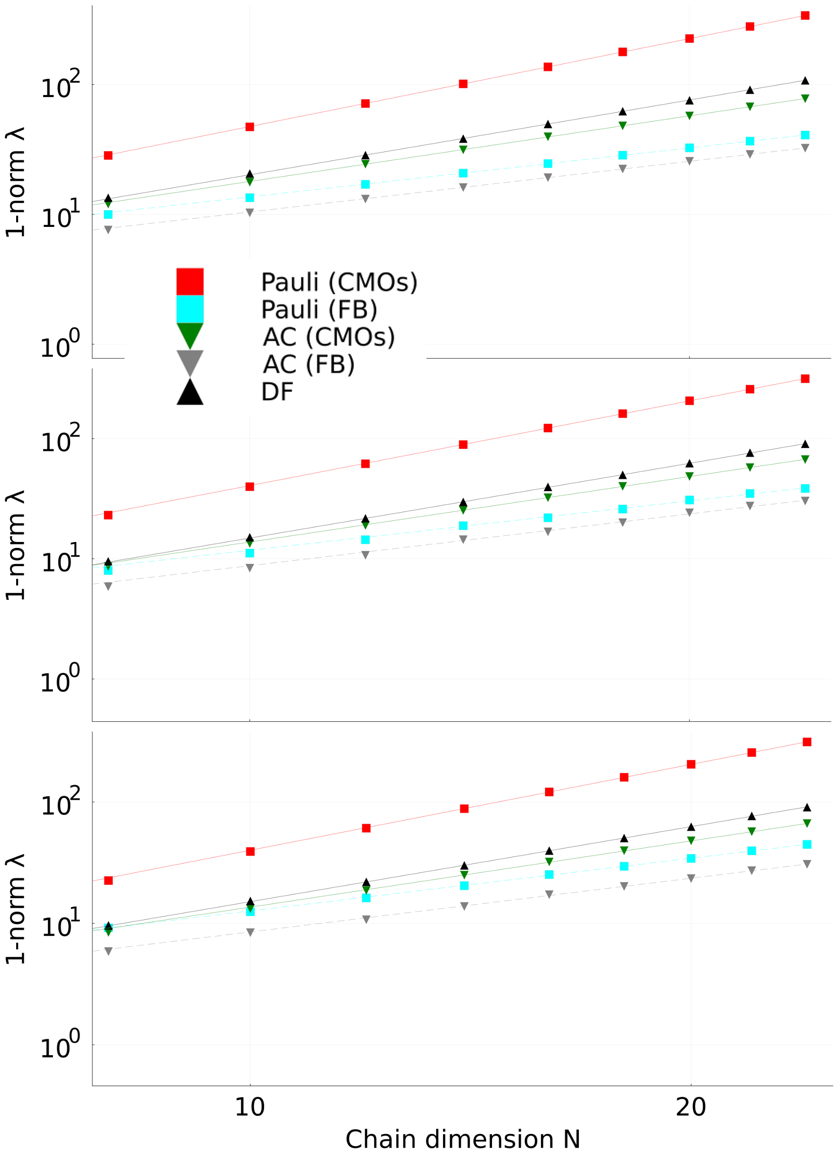
Figure 1: 1-norms scaling in hydrogen chains with $N$ atoms and spacing $r=1.4$ Å for various LCU s and different Hamiltonians (top: $\hat{H}$, middle: $\hat{H}_{S}$, bottom: $\hat{H}_{T}$). Lines correspond to polynomial scaling fit, where we consider $\log_{10}\lambda=\alpha\log_{10}N+\beta$. Fit coefficients are reported in Table 2. CMOs(FB) correspond to Hartree-Fock canonical molecular (Foster-Boys localized) orbitals.

For minimizing 1-norm of the Pauli product LCU of $\hat{H}_{T}(\vec{\kappa},\vec{\xi})$, we use a non-linear optimization package for the parameters $\vec{\kappa}$ and $\vec{\xi}$ Mogensen and Riseth (2018). Computational details of molecular electronic Hamiltonians and computational thresholds can be found in the Appendix. The orbital rotations for the orbital optimization scheme were obtained with a Broyden-Fletcher-Goldfarb-Shanno (BFGS) scheme for the Pauli LCU 1-norm in Table 1. For orbitals in the hydrogen chains we have used the Foster-Boys localization scheme Foster and Boys (1960). The Foster-Boys scheme is computationally more efficient than the orbital optimization that lowers 1-norm, while yielding 1-norm reductions that closely match the latter’s outcomes Koridon et al. (2021). The anticommuting groups were obtained using a sorted insertion algorithm Crawford et al. (2021); Izmaylov et al. (2020), and the double factorization (DF) fragments are found through a Cholesky decomposition of the two-electron tensor $g_{ijkl}$ Peng and Kowalski (2017); Motta et al. (2021, 2019); Matsuzawa and Kurashige (2020); Huggins et al. (2021); Lee et al. (2021). The Cartan sub-algebra (CSA) decomposition was done by obtaining fragments through a greedy optimization of their parameters one fragment at a time. The CSA decomposition was not calculated for the hydrogen chains because it quickly becomes prohibitively expensive as the system size grows.

Values in parenthesis in Table 1 represent the total number of unitaries in the LCU. Comparing the implementation costs of different LCUs is not a straightforward task, as the number and type of unitaries, in addition to the 1-norm, are linked to the implementation cost. Moreover, the specific form of the LCU decomposition can sometimes be used to construct more efficient circuits Lee et al. (2021); von Burg et al. (2021), necessitating the explicit construction of the oracle circuits for a comprehensive comparison of different LCUs. This is particularly noticeable for the DF method, with LCUs that have significantly less unitaries than the other decompositions but each unitary requires an implementation via qubitization. However, a full cost comparison of the quantum circuits is not necessary for showing the improvement from using BLISS. Within LCU-based encodings, the application of BLISS yielded reductions in 1-norm values while maintaining the number of unitaries nearly intact: following the BLISS procedure, there was an average decrease of approximately $2.2\%$ in the number of unitaries, with the maximum increase observed at $15.1\%$ for the NH₃ molecule with the orbital-optimized anticommuting grouping. Since the shifted Hamiltonian $\hat{H}_{T}$ has exactly the same operator form as $\hat{H}$, $\hat{H}$ and $\hat{H}_{T}$ can use the same compilation strategy. A similar number of unitaries in the LCU decompositions of $\hat{H}$ and $\hat{H}_{T}$ means that the only cost difference in their implementations will arise from the change of 1-norm.

We will refer to the previously developed shift technique Loaiza et al. (2023) as a partial shift, in contrast to a full shift that corresponds to the BLISS methodology and use of $\hat{H}_{T}$. We now start discussing the improvement of the spectral range $\Delta E$ when the BLISS is applied, having an average improvement of $31\%$ and $42\%$ with respect to the initial spectral range for the partial and full shifts respectively. This shows how the application of the BLISS will reduce significantly the quantum algorithm cost, requiring slightly more than half the resources of working with the full Hamiltonian $\hat{H}$.

For the Hamiltonian encoding cost, all presented methods show a very significant improvement when using the partial shift, while having an additional improvement when the full BLISS is used. Out of all studied methods, those with the best 1-norms are the orbital-optimized anticommuting grouping, and DF, presenting an average improvement of $49\%$ when compared to their unshifted versions, while the partial shift gave an average improvement of $38\%$ for DF and of $40\%$ for the orbital-optimized anticommuting grouping. As such, the BLISS technique practically halves the cost of implementing these LCU-based encodings.

From these results, it becomes clear that all of the previously mentioned energy estimation methods will greatly benefit from the application of the BLISS. If a Trotter-based method is used for implementing $f(\hat{H})=e^{-i\hat{H}t}$, the circuit cost and total run time will be reduced by $\sim 42\%$ for algorithms that re-scale the Hamiltonian Lin and Tong (2022). However, if $f(\hat{H})$ is to be implemented with an LCU-based method, the block-encoding LCU-based procedure encodes $f(\hat{H}/\lambda)$, which already has a normalized spectrum given how the 1-norm $\lambda\geq\Delta E/2$. Thus, the cost improvement from the encoding already incorporates the quantum algorithm cost reduction associated with re-scaling of $\hat{H}$. This results in a $\sim 49\%$ cost reduction for any LCU-based algorithms, while the partial shift yields an improvement of $38-40\%$ for the qubit and fermionic-based techniques presented in this work.

Furthermore, a comparison between the spectral range of the BLISS modified Hamiltonian and that of the original Hamiltonian in the subspace with $N_{e}$ electrons reveals remarkably similar values. This observation shows that the shift outlined in Eq.(9) cannot undergo significant further improvements: the BLISS procedure effectively eliminates contributions originating from subspaces with different number of electrons. Figure 1 and Table 2 illustrate the 1-norm scaling pattern for an extended chain of hydrogen atoms. The scaling of the 1-norms as a function of the chain length shown in Table 2 changes insignificantly after application of the shift, which indicates that the 1-norm improvement will likely exhibit similar behavior for large systems. While generalizing these trends to larger molecules with more flexible one-particle basis sets might be intricate, the substantial reduction in phase estimation algorithm costs resulting from the elimination of contributions associated with varying electron counts remains evident. The BLISS technique can be perceived as transitioning from the Hamiltonian in the complete Fock space to its counterpart within a fixed number of electrons subspace while remaining in a second quantization formalism. The question of whether first quantized Hamiltonians can similarly gain from symmetry shifts remains a topic under ongoing exploration.

We note that combining the BLISS technique with the previously proposed interaction picture methodology Loaiza et al. (2023); Low and Wiebe (2019) did not give any additional improvements to the unshifted interaction picture, following the same rationale as the previously proposed symmetry shift. For a more detailed discussion, see Ref. 23.

IV Conclusions

We have presented the BLISS methodology for more efficient encodings of the moleculular electronic structure Hamiltonians. The key idea of BLISS is the modification of $\hat{H}$ that reduces its spectral range and 1-norm LCU cost without changing its action in the Fock subspace of a particular molecular symmetry. By substituting $\hat{H}$ with a modified operator $\hat{H}_{T}$ in the energy estimation algorithm lowers the overall cost without affecting results. The target number of electrons, which is used when constructing $\hat{H}_{T}$, is specified when an initial wavefunction is considered in the energy estimation algorithm. Alternatively, even if the initial wavefunction is not an eigenstate of the electron number operator, the ground state energy can still be recovered as long as the overlap with the ground state is larger than the overlap with any other eigenstate. The BLISS methodology yields a shifted Hamiltonian $\hat{H}_{T}$ of the same operator form as the original two-electron Hamiltonian $\hat{H}$ [Eq.(5)], the only difference is in modified electron-integral coefficients. As such, this methodology can be used as a preprocessing step for any electronic structure Hamiltonian, and can be thought as obtaining a “new molecule” that is isospectral to $\hat{H}$ in the subspace with a target number of electrons. The $2.2\%$ average decrease in the required number of unitaries for the LCU decompositions after the symmetry shift means that the only factor modifying the cost of the phase estimation algorithm will be the change in 1-norm of the shifted Hamiltonian.

Application of the BLISS reduced 1-norms of LCU encodings by a factor $\sim 2$ and spectral ranges of electronic Hamiltonians by a factor of $\sim 1.7$. This practically halves the cost of energy estimation routines on a quantum computer.

Appendix A Appendix A: LCU decompositions

Here we review the different LCU decompositions that were used in this work.

A.0.1 Qubit-based approaches

The simplest LCU decomposition is obtained when $\hat{H}$ is mapped into a qubit operator by means of a fermion-to-qubit mapping, e.g. Jordan-Wigner Wigner and Jordan (1928) or Bravyi-Kitaev Bravyi and Kitaev (2002); Seeley et al. (2012); Tranter et al. (2015). This yields the expression

$$\hat{H}=\sum_{q}d_{q}\hat{P}_{q},$$ (10)

where $d_{q}$ are constants and $\hat{P}_{q}$ are Pauli-product operators consisting of products of Pauli matrices acting on different qubits. Given how $\hat{P}_{q}$’s are already unitary, this expression is already an LCU of the Hamiltonian with the 1-norm

$$\lambda^{(P)}=\sum_{q}|d_{q}|.$$ (11)

We note that by expressing the Hamiltonian using Majorana operators, this 1-norm can also be obtained as a function of the fermionic tensors Koridon et al. (2021); Loaiza et al. (2023):

$$\lambda^{(P)} =\sum_{ij}|h_{ij}+2\sum_{k}g_{ijkk}|+\sum_{i>k,j>l}|g_{ijkl}-g_{ilkj}|$$

$$\ +\frac{1}{2}\sum_{ijkl}|g_{ijkl}|.$$ (12)

When starting from the qubit Hamiltonian [Eq.(10)], there are two additional optimizations that can be done for lowering the encoding cost. The orbital optimization technique Koridon et al. (2021) applies an orbital rotation

$$\hat{U}(\vec{\theta})\equiv\prod_{i>j}e^{\theta_{ij}(\hat{F}^{i}_{j}-\hat{F}_{i}^{j})},$$ (13)

finding the optimal parameters $\vec{\theta}$ such that the 1-norm of $\hat{U}(\vec{\theta})\hat{H}\hat{U}^{\dagger}(\vec{\theta})$ is minimized. In addition, we can also make use of the anticommuting grouping technique Izmaylov et al. (2020); Loaiza et al. (2023). The key idea of this approach is that a normalized linear combination of mutually anticommuting Pauli products yields a unitary operator. Noting that two arbitrary Pauli products $\hat{P}_{i}$ and $\hat{P}_{j}$ always either commute ($[\hat{P}_{i},\hat{P}_{j}]=0$) or anticommute ($\{\hat{P}_{i},\hat{P}_{j}\}=0$), mutually anticommuting Pauli products are grouped into sets with corresponding indices $G_{n}$. We thus obtain the LCU

$$\hat{H}=\sum_{n}a_{n}\hat{A}_{n},$$ (14)

where $\hat{A}_{n}\equiv\frac{1}{a_{n}}\sum_{q\in G_{n}}d_{q}\hat{P}_{q}$ are unitary operators and $a_{n}\equiv\sqrt{\sum_{q\in G_{n}}|d_{q}|^{2}}$. It can be easily shown Loaiza et al. (2023) that the resulting 1-norm of this decomposition,

$$\lambda^{(AC)}=\sum_{n}|a_{n}|$$ (15)

is always smaller than $\lambda^{(P)}$ if there is a nontrivial grouping.

A.0.2 Fermionic-based approaches

We now give an overview of fermionic-based approaches. We start by giving the CSA form of the Hamiltonian Yen and Izmaylov (2021); Cohn et al. (2021); Oumarou et al. (2022):

$$\hat{H}_{1} \equiv\sum_{ij}h_{ij}\hat{F}^{i}_{j}$$ (16)

$$=\hat{U}_{1}\left(\sum_{i}\lambda_{ii}^{(1)}\sum_{\sigma}\hat{n}_{i\sigma}\right)\hat{U}_{1}^{\dagger},$$ (17)

and

$$\hat{H}_{2} \equiv\sum_{ijkl}g_{ijkl}\hat{F}^{i}_{j}\hat{F}^{k}_{l}$$ (18)

$$=\sum_{m\geq 2}\hat{U}_{m}\left(\sum_{ij}\lambda_{ij}^{(m)}\sum_{\sigma\tau}\hat{n}_{i\sigma}\hat{n}_{j\tau}\right)\hat{U}_{m}^{\dagger},$$ (19)

where we have defined the one(two)-electron Hamiltonians $\hat{H}_{1(2)}$ such that $\hat{H}=\hat{H}_{1}+\hat{H}_{2}$, $\{\sigma,\tau\}$ correspond to $z$-spin projections $\{\alpha,\beta\}$, $\hat{n}_{i\sigma}\equiv\hat{a}^{\dagger}_{i\sigma}\hat{a}_{i\sigma}$ is the number operator on orbital $i$ with spin $\sigma$, and $\hat{U}_{m}$’s are orbital rotations as seen in Eq.(13). By noting that the number operators $\hat{n}_{i\sigma}$ can be mapped into reflections, and thus unitaries, by the transformation $\hat{n}_{i\sigma}\rightarrow 2\hat{n}_{i\sigma}-\hat{1}$. Defining the reflections $\hat{r}_{i\sigma}\equiv 2\hat{n}_{i\sigma}-\hat{1}$, the CSA form of the Hamiltonian can be turned into an LCU as

$$\hat{H}_{2}^{\textrm{(LCU)}}=\sum_{m}\hat{U}_{m}\left(\sum_{ij}\frac{\lambda_{ij}^{(m)}}{4}\sum_{\sigma\tau}\hat{r}_{i\sigma}\hat{r}_{j\tau}\right)\hat{U}_{m}^{\dagger}.$$ (20)

An adjustment of $\hat{H}_{1}$ must be done to account for the one-electron terms coming from the $\hat{n}_{i\sigma}\rightarrow\hat{r}_{i\sigma}$ mapping, which can be shown to yield Lee et al. (2021)

$$\hat{H}_{1}^{\prime}\equiv\hat{H}_{1}+2\sum_{ijk}g_{ijkk}\hat{F}^{i}_{j}.$$ (21)

This one-electron operator can then be diagonalized as $\hat{H}_{1}^{\prime}=\hat{U}_{1}^{\prime}\left(\sum_{i}\mu_{i}\sum_{\sigma}\hat{n}_{i\sigma}\right)\hat{U}_{1}^{\prime\dagger}$, obtaining the LCU

$$\hat{H}_{1}^{(\textrm{LCU})}=\hat{U}_{1}^{\prime}\left(\sum_{i}\frac{\mu_{i}}{2}\sum_{\sigma}\hat{r}_{i\sigma}\right)\hat{U}_{1}^{\prime\dagger}.$$ (22)

The resulting 1-norm of this decomposition then corresponds to

$$\lambda^{(\textrm{CSA})} =\lambda_{1}+\lambda_{2}^{(\textrm{CSA})}$$

$$=\sum_{i}|\mu_{i}|+\sum_{m\geq 2}\sum_{ij}|\lambda^{(m)}_{ij}|-\frac{1}{2}\sum_{m\geq 2}\sum_{i}|\lambda^{(m)}_{ii}|,$$ (23)

where we have removed some operators associated with the $\lambda_{ii}^{(m)}$ coefficients due to the fact that $\hat{r}_{i\sigma}^{2}=\hat{1}$. Note that the modified one-electron fragment is independent of the fermionic LCU decomposition method.

An alternative LCU decomposition can be made through the DF decomposition von Burg et al. (2021); Berry et al. (2019); Peng and Kowalski (2017); Motta et al. (2021, 2019); Matsuzawa and Kurashige (2020); Huggins et al. (2021), which can be considered as a CSA decomposition with a rank-deficient tensor $\lambda_{ij}^{(m)}=\epsilon^{(m)}_{i}\epsilon^{(m)}_{j}$. This allows for the Hamiltonian to be written as

$$\hat{H}_{2}=\sum_{m}\hat{U}_{m}\left(\sum_{i}\epsilon_{i}^{(m)}\sum_{\sigma}\hat{n}_{i\sigma}\right)^{2}\hat{U}_{m}^{\dagger}.$$ (24)

The complete-square structure of each fragment then allows for the implementation of each $m$-th fragment as a single unitary through the use of a qubitization procedure Berry et al. (2019); Lee et al. (2021), yielding a correspoding 1-norm of

$$\lambda^{(\textrm{DF})} =\lambda_{1}+\lambda_{2}^{(\textrm{DF})}$$ (25)

$$=\sum_{i}|\mu_{i}|+\frac{1}{2}\sum_{m\geq 2}\left(\sum_{i}\epsilon_{i}^{(m)}\right)^{2}.$$ (26)

For a more detailed discussion of how the DF LCU is implemented, we refer to Refs. 24; 23; 14.

Finally, we note that we have skipped the Tensor Hypercontraction method Lee et al. (2021); Rubin et al. (2023) for LCU decompositions. This is due to the current optimization procedures for this decomposition being unstable and having a poor convergence to $\hat{H}$: the non-linear nature of this ansatz makes the optimization extremely sensitive to initial conditions and to the chosen optimization method. Work for obtaining this decomposition in a robust and stable way is under progress.

Appendix B Appendix B: Molecular geometries and computational details

In this section we write down all details necessary for numerical reproducibility. Our code is available at https://github.com/iloaiza/QuantumMAMBO.jl.

For the CSA decompositions of the two-electron tensor, the cost function was chosen as the 2-norm of $\Delta\hat{H}\equiv\sum_{ijkl}b_{ijkl}\hat{F}^{i}_{j}\hat{F}^{k}_{l}$:

$$||\Delta\hat{H}||_{2}\equiv\sum_{ijkl}|b_{ijkl}|^{2},$$ (27)

considering the decomposition finished when this norm is below a tolerance of $1\times 10^{-6}$. All non-linear optimizations where done using the Julia Optim.jl package Mogensen and Riseth (2018), using the BFGS algorithm Fletcher (2000) with the default tolerance. Linear programming routines were done using the Julia JuMP package Dunning et al. (2017) with the HiGHS optimizer Huangfu and Hall (2018).

All molecular Hamiltonians were generated using the PySCF package Sun (2015); Sun et al. (2018, 2020) and the Openfermion library McClean et al. (2020), using a minimal STO-3G basis Hehre et al. (1969); Szabo and Ostlund (1996) and the Jordan-Wigner transformation Wigner and Jordan (1928). The nuclear geometries for the Hamiltonians are:

• R(H – H) = $1\textrm{\AA}$ for H₂

• R(Li – H) = $1\textrm{\AA}$ for LiH

• R(Be – H) = $1\textrm{\AA}$ with a collinear atomic arrangement for BeH₂

• R(O – H) = $1\textrm{\AA}$ with angle $\angle$HOH = $107.6^{\circ}$ for H₂O

• R(N – H) = $1\textrm{\AA}$ with $\angle$HNH = $107^{\circ}$ for NH₃

References

- Cao et al. (2019) Y. Cao, J. Romero, J. P. Olson, M. Degroote, P. D. Johnson, M. Kieferová, I. D. Kivlichan, T. Menke, B. Peropadre, N. P. D. Sawaya, S. Sim, L. Veis, and A. Aspuru-Guzik, Chem. Rev. 119, 10856 (2019).
- Kassal et al. (2008) I. Kassal, S. P. Jordan, P. J. Love, M. Mohseni, and A. Aspuru-Guzik, Proc. Natl. Acad. Sci. 105, 18681 (2008).
- Abrams and Lloyd (1999) D. S. Abrams and S. Lloyd, Phys. Rev. Lett. 83, 5162 (1999).
- Kitaev (1995) A. Y. Kitaev, “Quantum measurements and the Abelian stabilizer problem,” (1995), arXiv:9511026 [quant-ph] .
- Aspuru-Guzik et al. (2005) A. Aspuru-Guzik, A. D. Dutoi, P. J. Love, and M. Head-Gordon, Science 309, 1704 (2005).
- Lin and Tong (2022) L. Lin and Y. Tong, PRX Quantum 3, 010318 (2022).
- Moore et al. (2021) A. J. Moore, Y. Wang, Z. Hu, S. Kais, and A. M. Weiner, New J. Phys. 23, 113027 (2021).
- Somma (2019) R. D. Somma, New J. Phys. 21, 123025 (2019).
- Ge et al. (2019) Y. Ge, J. Tura, and J. I. Cirac, J. Math. Phys. 60, 022202 (2019).
- Wang et al. (2022) G. Wang, D. Stilck-França, R. Zhang, S. Zhu, and P. D. Johnson, “Quantum algorithm for ground state energy estimation using circuit depth with exponentially improved dependence on precision,” (2022).
- Childs and Wiebe (2012) A. M. Childs and N. Wiebe, Quantum Info. Comput. 12, 901–924 (2012).
- Low and Wiebe (2019) G. H. Low and N. Wiebe, “Hamiltonian simulation in the interaction picture,” (2019), arXiv:1805.00675 [quant-ph] .
- Berry et al. (2019) D. W. Berry, C. Gidney, M. Motta, J. R. McClean, and R. Babbush, Quantum 3, 208 (2019).
- Lee et al. (2021) J. Lee, D. W. Berry, C. Gidney, W. J. Huggins, J. R. McClean, N. Wiebe, and R. Babbush, PRX Quantum 2, 030305 (2021).
- Suzuki (1991) M. Suzuki, J. Math. Phys. 32, 400 (1991).
- Low and Chuang (2019) G. H. Low and I. L. Chuang, Quantum 3, 163 (2019).
- Babbush et al. (2018) R. Babbush, C. Gidney, D. W. Berry, N. Wiebe, J. McClean, A. Paler, A. Fowler, and H. Neven, Phys. Rev. X 8, 041015 (2018).
- Delgado et al. (2022) A. Delgado, P. A. M. Casares, R. dos Reis, M. S. Zini, R. Campos, N. Cruz-Hernández, A.-C. Voigt, A. Lowe, S. Jahangiri, M. A. Martin-Delgado, J. E. Mueller, and J. M. Arrazola, Phys. Rev. A 106, 032428 (2022).
- Rubin et al. (2023) N. C. Rubin, D. W. Berry, F. D. Malone, A. F. White, T. Khattar, A. E. DePrince, S. Sicolo, M. Kühn, M. Kaicher, J. Lee, and R. Babbush, “Fault-tolerant quantum simulation of materials using bloch orbitals,” (2023), arXiv:2302.05531 [quant-ph] .
- Steudtner et al. (2023) M. Steudtner, S. Morley-Short, W. Pol, S. Sim, C. L. Cortes, M. Loipersberger, R. M. Parrish, M. Degroote, N. Moll, R. Santagati, and M. Streif, “Fault-tolerant quantum computation of molecular observables,” (2023), arXiv:2303.14118 [quant-ph] .
- Kim et al. (2022) I. H. Kim, Y.-H. Liu, S. Pallister, W. Pol, S. Roberts, and E. Lee, Phys. Rev. Res. 4, 023019 (2022).
- Goings et al. (2022) J. J. Goings, A. White, J. Lee, C. S. Tautermann, M. Degroote, C. Gidney, T. Shiozaki, R. Babbush, and N. C. Rubin, Proc. Natl. Acad. Sci. 119 (2022).
- Loaiza et al. (2023) I. Loaiza, A. M. Khah, N. Wiebe, and A. F. Izmaylov, Quantum Sci. Tech. 8, 035019 (2023).
- von Burg et al. (2021) V. von Burg, G. H. Low, T. Haner, D. Steiger, M. Reiher, M. Roetteler, and M. Troyer, Phys. Rev. Research 3, 033055 (2021).
- Campbell (2021) E. T. Campbell, Quantum Sci. Tech. 7, 015007 (2021).
- Setia et al. (2020) K. Setia, R. Chen, J. E. Rice, A. Mezzacapo, M. Pistoia, and J. D. Whitfield, J. Chem. Theor. Comput. 16, 6091 (2020).
- Peruzzo et al. (2014) A. Peruzzo, J. McClean, P. Shadbolt, M.-H. Yung, X.-Q. Zhou, P. J. Love, A. Aspuru-Guzik, and J. L. O’Brien, Nature Comm. 5 (2014).
- Anand et al. (2022) A. Anand, P. Schleich, S. Alperin-Lea, P. W. K. Jensen, S. Sim, M. Dí az-Tinoco, J. S. Kottmann, M. Degroote, A. F. Izmaylov, and A. Aspuru-Guzik, Chem. Soc. Rev. 51, 1659 (2022).
- Tilly et al. (2022) J. Tilly, H. Chen, S. Cao, D. Picozzi, K. Setia, Y. Li, E. Grant, L. Wossnig, I. Rungger, G. H. Booth, and J. Tennyson, Phys. Rep. 986, 1 (2022).
- Romero et al. (2018) J. Romero, R. Babbush, J. R. McClean, C. Hempel, P. Love, and A. Aspuru-Guzik, “Strategies for quantum computing molecular energies using the unitary coupled cluster ansatz,” (2018), arXiv:1701.02691 [quant-ph] .
- Ryabinkin et al. (2018) I. G. Ryabinkin, T.-C. Yen, S. N. Genin, and A. F. Izmaylov, J. Chem. Theor. Comput. 14, 6317 (2018).
- Malz et al. (2023) D. Malz, G. Styliaris, Z.-Y. Wei, and J. I. Cirac, “Preparation of matrix product states with log-depth quantum circuits,” (2023), arXiv:2307.01696 [quant-ph] .
- White (1992) S. R. White, Phys. Rev. Lett. 69, 2863 (1992).
- Schollwöck (2011) U. Schollwöck, Annals Phys. 326, 96 (2011).
- Chan and Sharma (2011) G. K.-L. Chan and S. Sharma, Annual Rev. Phys. Chem. 62, 465 (2011).
- Silvi et al. (2012) P. Silvi, D. Rossini, R. Fazio, G. E. Santoro, and V. Giovannetti, Int. J. Mod. Phys. B 27, 1345029 (2012).
- Koridon et al. (2021) E. Koridon, S. Yalouz, B. Senjean, F. Buda, T. E. O’Brien, and L. Visscher, Phys. Rev. Research 3, 033127 (2021).
- Mogensen and Riseth (2018) P. K. Mogensen and A. N. Riseth, J. Open Source Softw. 3, 615 (2018).
- Foster and Boys (1960) J. M. Foster and S. F. Boys, Rev. Mod. Phys. 32, 300 (1960).
- Crawford et al. (2021) O. Crawford, B. van Straaten, D. Wang, T. Parks, E. Campbell, and S. Brierley, Quantum 5, 385 (2021).
- Izmaylov et al. (2020) A. F. Izmaylov, T.-C. Yen, R. A. Lang, and V. Verteletskyi, J. Chem. Theor. Comput. 16, 190 (2020).
- Peng and Kowalski (2017) B. Peng and K. Kowalski, J. Chem. Theor. Comput. 13, 4179 (2017).
- Motta et al. (2021) M. Motta, E. Ye, J. R. McClean, Z. Li, A. J. Minnich, R. Babbush, and G. K.-L. Chan, npj Quantum Info. 7, 83 (2021).
- Motta et al. (2019) M. Motta, J. Shee, S. Zhang, and G. K.-L. Chan, J. Chem. Theor. Comput. 15, 3510 (2019).
- Matsuzawa and Kurashige (2020) Y. Matsuzawa and Y. Kurashige, J. Chem. Theor. Comput. 16, 944 (2020).
- Huggins et al. (2021) W. J. Huggins, J. R. McClean, N. C. Rubin, Z. Jiang, N. Wiebe, K. B. Whaley, and R. Babbush, npj Quantum Info. 7, 23 (2021).
- Wigner and Jordan (1928) E. Wigner and P. Jordan, Z. Phys 47, 631 (1928).
- Bravyi and Kitaev (2002) S. B. Bravyi and A. Y. Kitaev, Ann. Phys. 298, 210 (2002).
- Seeley et al. (2012) J. T. Seeley, M. J. Richard, and P. J. Love, J. Chem. Phys. 137, 224109 (2012).
- Tranter et al. (2015) A. Tranter, S. Sofia, J. Seeley, M. Kaicher, J. McClean, R. Babbush, P. V. Coveney, F. Mintert, F. Wilhelm, and P. J. Love, Int. J. Quantum Chem. 115, 1431 (2015).
- Yen and Izmaylov (2021) T.-C. Yen and A. F. Izmaylov, PRX Quantum 2, 040320 (2021).
- Cohn et al. (2021) J. Cohn, M. Motta, and R. M. Parrish, PRX Quantum 2, 040352 (2021).
- Oumarou et al. (2022) O. Oumarou, M. Scheurer, R. M. Parrish, E. G. Hohenstein, and C. Gogolin, “Accelerating quantum computations of chemistry through regularized compressed double factorization,” (2022), arXiv:2212.07957 [quant-ph] .
- Fletcher (2000) R. Fletcher, Practical Methods of Optimization (John Wiley & Sons, West Sussex, England, 2000).
- Dunning et al. (2017) I. Dunning, J. Huchette, and M. Lubin, SIAM Review 59, 295 (2017).
- Huangfu and Hall (2018) Q. Huangfu and J. Hall, Math. Prog. Comput. 10, 119–142 (2018).
- Sun (2015) Q. Sun, J. Comput. Chem. 36, 1664 (2015).
- Sun et al. (2018) Q. Sun, T. C. Berkelbach, N. S. Blunt, G. H. Booth, S. Guo, Z. Li, J. Liu, J. D. McClain, E. R. Sayfutyarova, S. Sharma, S. Wouters, and G. K.-L. Chan, WIREs Comput. Mol. Sci. 8, e1340 (2018).
- Sun et al. (2020) Q. Sun, X. Zhang, S. Banerjee, P. Bao, M. Barbry, N. S. Blunt, N. A. Bogdanov, G. H. Booth, J. Chen, Z.-H. Cui, J. J. Eriksen, Y. Gao, S. Guo, J. Hermann, M. R. Hermes, K. Koh, P. Koval, S. Lehtola, Z. Li, J. Liu, N. Mardirossian, J. D. McClain, M. Motta, B. Mussard, H. Q. Pham, A. Pulkin, W. Purwanto, P. J. Robinson, E. Ronca, E. R. Sayfutyarova, M. Scheurer, H. F. Schurkus, J. E. T. Smith, C. Sun, S.-N. Sun, S. Upadhyay, L. K. Wagner, X. Wang, A. White, J. D. Whitfield, M. J. Williamson, S. Wouters, J. Yang, J. M. Yu, T. Zhu, T. C. Berkelbach, S. Sharma, A. Y. Sokolov, and G. K.-L. Chan, J. Chem. Phys. 153, 024109 (2020).
- McClean et al. (2020) J. R. McClean, N. C. Rubin, K. J. Sung, I. D. Kivlichan, X. Bonet-Monroig, Y. Cao, C. Dai, E. S. Fried, C. Gidney, B. Gimby, P. Gokhale, T. Häner, T. Hardikar, V. Havlíček, O. Higgott, C. Huang, J. Izaac, Z. Jiang, X. Liu, S. McArdle, M. Neeley, T. O’Brien, B. O’Gorman, I. Ozfidan, M. D. Radin, J. Romero, N. P. D. Sawaya, B. Senjean, K. Setia, S. Sim, D. S. Steiger, M. Steudtner, Q. Sun, W. Sun, D. Wang, F. Zhang, and R. Babbush, Quantum Sci. Tech. 5, 034014 (2020).
- Hehre et al. (1969) W. J. Hehre, R. F. Stewart, and J. A. Pople, J. Chem. Phys. 51, 2657 (1969).
- Szabo and Ostlund (1996) A. Szabo and N. Ostlund, Modern Quantum Chemistry: Introduction to Advanced Electronic Structure Theory, Dover Books on Chemistry (Dover Publications, Mineola, New York, USA, 1996).