Phagocytosis Unveiled:
A Scalable and Interpretable Deep learning Framework for Neurodegenerative Disease Analysis

Abstract

Quantifying the phagocytosis of dynamic, unstained cells is essential for evaluating neurodegenerative diseases. However, measuring rapid cell interactions and distinguishing cells from backgrounds make this task challenging when processing time-lapse phase-contrast video microscopy. In this study, we introduce a fully automated, scalable, and versatile real-time framework for quantifying and analyzing phagocytic activity. Our proposed pipeline can process large data-sets and includes a data quality verification module to counteract potential perturbations such as microscope movements and frame blurring. We also propose an explainable cell segmentation module to improve the interpretability of deep learning methods compared to black-box algorithms. This includes two interpretable deep learning capabilities: visual explanation and model simplification. We demonstrate that interpretability in deep learning is not the opposite of high performance, but rather provides essential deep learning algorithm optimization insights and solutions. Incorporating interpretable modules results in an efficient architecture design and optimized execution time. We apply this pipeline to quantify and analyze microglial cell phagocytosis in frontotemporal dementia (FTD) and obtain statistically reliable results showing that FTD mutant cells are larger and more aggressive than control cells. To stimulate translational approaches and future research, we release an open-source pipeline and a unique microglial cells phagocytosis dataset for immune system characterization in neurodegenerative diseases research. This pipeline and dataset will consistently crystallize future advances in this field, promoting the development of efficient and effective interpretable algorithms dedicated to this critical domain. https://github.com/ounissimehdi/PhagoStat

Introduction

The latest advances in physics, especially in high-throughput microscopy, along with computer-aided analysis, are opening up a new frontier in fundamental cellular understanding in biology. The progress made in this field is due to the automation of formerly labor-intensive tasks, such as identifying cells, counting them, tracking their movements, and profiling their characteristics [1, 2, 3].

These developments have significant implications for numerous biological experiments that explore the dynamics and the behavior of immune cells. In particular, the process of phagocytosis, in which microglial cells engulf and eliminate protein deposits or aggregates, has garnered significant attention in the field of neurodegenerative diseases [4, 5, 6, 7, 8]. A deeper understanding of this phenomenon is essential for elucidating the complex mechanisms underlying these disorders and their progression. Consequently, there is a growing demand for more precise and accurate quantitative methods to advance the field, as they can offer invaluable insights into the interplay between microglial cells and protein aggregates, ultimately contributing to the development of novel therapeutic strategies and interventions for neurodegenerative diseases.

While traditional image processing methods have been used in microscopy to detect cells [9], they often struggle to accurately detect unstained cells, measure rapid cell interactions, and distinguish cells from their background in a complex setting. To address these challenges, innovative approaches that utilize the latest advances in computer vision (CV) and deep learning (DL) are required [10, 11].

Fortunately, DL has brought substantial improvements to cell segmentation, offering several advanced models including U-Net, Mask R-CNN, DeepLabv3+, Stardist, and Cellpose, which have been widely adopted for various segmentation tasks [12, 13, 14, 15, 16].

However, the opaqueness of black-box algorithms presents a major obstacle to their adoption in clinical settings. Therefore, it is important to reveal the inner workings of DL models and promote transparency [17, 18] to build trust in using advanced technology. Consequently, the development of interpretable DL-based tools can encourage their adoption, potentially leading to further discoveries in these fields.

Despite the potential of DL-based approaches for quantifying cell phagocytosis, to our knowledge, there is currently no existing ready-made open-source solution capable of effectively handling this task under real-world conditions. To address this, we present PhagoStat, a scalable pipeline utilizing interpretable DL and open-source packages to enhance our understanding of cell phagocytosis. This tool integrates DL precision with explainable artificial intelligence (XAI) transparency, emphasizing interpretability in cell biology research. PhagoStat streamlines essential cellular feature extraction, providing a comprehensive, accessible solution for researchers and advancing our knowledge of cellular processes, particularly phagocytosis.

The principal contributions of our work can be outlined as follows:

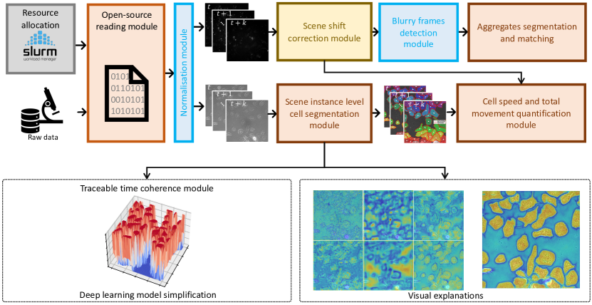
Figure 1: PhagoStat: A comprehensive pipeline for quantifying microglial cell phagocytosis in the context of frontotemporal dementia (FTD). The PhagoStat pipeline is a fully operational system comprised of the following stages: (i) efficient loading of raw data (Fig.2.b), (ii) applying data quality checks and quantifying aggregates over time (Fig 3.c), and (iii) performing cell instance segmentation using an interpretable deep learning (IDL) approach (Fig.5, which incorporates Fig.4.c). This comprehensive pipeline streamlines the analysis process and facilitates accurate and reliable results for researchers working with microglial cell phagocytosis data.

1. The PhagoStat pipeline, illustrated in Fig. 1, is a flexible framework comprising of several interconnected and interchangeable modules designed to analyze unstained cells overlaid on fluorescent aggregates. It handles data-sequence loading and normalization, video-based registration and frame alignment, noise detection and removal, aggregate and cellular quantification, and statistical reporting. By streamlining the analysis process, these modules ensure precise results, preserve data integrity, leverage interpretable DL for cellular segmentation, and provide clear statistical insights into cell activity under different experimental conditions.

2. We showcase a comprehensive use case of the PhagoStat pipeline applied to microglial cells. Our analysis yields statistically significant results, uncovering a crucial finding: Frontotemporal Dementia (FTD) mutant cells display both larger size and increased activity in comparison to their control counterparts (refer to section 1.2). This important discovery demonstrates the potential of the PhagoStat pipeline in advancing our understanding of neurodegenerative diseases and promoting further research in this critical field.

3. We are releasing a large dataset that focuses on the phagocytosis of microglial cells. The dataset includes ten videos captured over a 7-hour period. Each video containing 20 simultaneous scenes, with both WT and FTD mutants cells in the context of FTD. The aggregates are fluorescent, while the cells are unstained. The purpose of releasing this dataset is to facilitate further understanding and application of our pipeline. The dataset comprises 36,496 cell images and 1,306,131 cell masks, along with 36,496 aggregate images and 1,553,036 aggregate masks, promoting further research into microglial cell phagocytosis.

1 Results

1.1 Phagocytosis quantification pipeline

The pipeline consists of several interconnected modules, each tailored to perform specific tasks effectively.

Firstly, we introduce the data-efficient loading and normalization module (refer to 1.1.1), which ensures streamlined data handling and preprocessing. This module is crucial for reducing the computational burden and facilitating subsequent analysis.

Secondly, we elaborate on the spatiotemporal frame registration process, which is accompanied by a data quality check (refer to 1.1.2). This step incorporates scene shift correction and blurry frame detection, ensuring the accuracy and reliability of the acquired data while maintaining spatial and temporal alignment across frames.

Thirdly, We introduce the cellular and aggregate quantification modules (refer to 1.1.3) designed to offer a comprehensive analysis of cellular properties and interactions. The first module employs instance-level interpretable segmentation techniques, effectively extracting and analyzing cellular properties from unstained cell images. This approach allows for an in-depth examination of individual cell behavior and morphology. Concurrently, a second module utilizes advanced image processing techniques to facilitate accurate aggregate segmentation and matching from fluorescent aggregate images. These techniques provide insights into the complex interactions between cells and aggregates, revealing crucial biological and morphological features.

Finally, the pipeline integrates the information obtained from both aggregates and cells. By quantifying phagocytosis, this module provides a comprehensive projection of the entire framework, showcasing the applicability of PhagoStat pipeline in the phagocytosis research contexts.

1.1.1 Data efficient loading and normalization

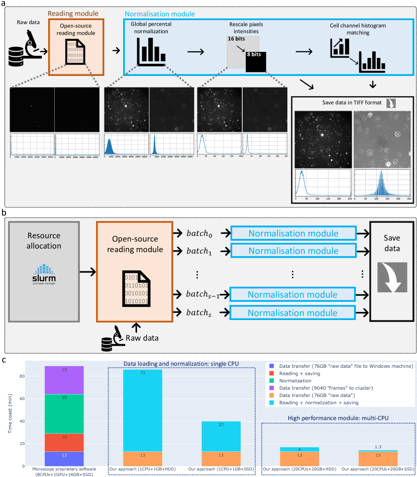
Figure 2: Efficient data loading and normalization pipeline. (a) Detailed steps of the data loading and normalization module where: the two channels (aggregates and cells) are extracted directly from the microscope raw data, then it applies the local and global normalization to standardize the data. (b) High performance computing (HPC) cluster compatible scheme that scales to big datasets. (c) Quantitative evaluation of our approach using single-CPU/multi-CPUs compared to the GPU-accelerated Carl Zeiss Microscopy ZEN software.

We would like to emphasize that this module is not designed exclusively for a specific microscope or proprietary software. Instead, it presents a versatile and general approach that can be readily applied to any microscope system. This use case serves to demonstrate the effectiveness of the module, which was implemented using open-source packages, with further details provided in the Methods section. Our findings illustrate that our approach is at least two times faster than commonly used proprietary software while requiring only 1/8 of the hardware resources, as shown in Fig. 2.c.

Following a thorough evaluation, we observed that the combination of percentile normalization (tailored to each sequence, referred to as "global normalization") and cumulative histogram distribution matching (tailored to each image, referred to as "local normalization") is highly effective in reducing data variability. This dual normalization strategy enhances the performance of DL segmentation model, resulting in up to a 10% improvement in the dice coefficient. Moreover, we integrated this normalization approach with the raw data readout module, capitalizing on its parallelism scheme. This integration substantially reduces the time cost associated with various processes, such as reading raw data, normalizing data, and saving normalized data, as opposed to adding a separate normalization module after data readout (e.g., reading raw data, saving it in an open format, loading saved data, normalizing data, and saving normalized data).

1.1.2 Data quality check for scene shift correction and blurry frames rejection

During our analysis of high-content video-microscopy recordings captured over extended periods, we observed the presence of several unavoidable hardware-related acquisition faults or artifacts. One such artifact was the unintended shaking of the microscope along the x and y axes. These imperfections, although localized to specific frames, had a detrimental impact on the overall sequence quality. Consequently, these artifacts can potentially compromise the accuracy and reliability of subsequent data analysis and interpretation, underscoring the importance of addressing such issues in a systematic manner during the data processing stage.

In our study, we aimed to investigate how external disturbances affect the performance of the microscope camera sensor. To this end, we recorded 20 simultaneous scenes, each containing two channels (cells:non-fluorescent and aggregates:fluorescent), with a frequency of 1 frame every 2 minutes, over a period of 7 hours without any interruption. During the recording process, we estimated that the microscope camera sensor had only 6 seconds (2 min divided by 20 scenes) to cycle and stabilize along the x and y axes from frame n to frame n+1 to capture pixel intensities and write them to a local disk.

However, external disturbances, such as mechanical vibrations, lens getting out of focus, can cause the microscope camera sensor to deviate from its normal performance, further reducing the time-response gap. Likely, such external disturbances occur at least once during the 7h non-stop sessions. When this happened, it affected the quality of 1 to 10 consecutive frames.

In order to counteract the potential influence of external disturbances on our analysis, we developed a registration-based module specifically designed to align and stabilize the frames. This module effectively mitigates any potential deviations caused by external factors, ensuring the accuracy and reliability of the subsequent data analysis.

It is important to note that in the aggregate channel, the majority of pixels belong to the background. This predominance of low-intensity pixels (i.e., the background) in comparison to the high-intensity pixels (i.e., the aggregate) presents a significant challenge when it comes to registration (offset correction).

Given the explainable nature of our pipeline, we opted against using black-box registration approaches based on DL [19]. Instead, we chose to employ the Scale-Invariant Feature Transform (SIFT) algorithm [20] as our registration method. SIFT is not only fully explainable and mature, but it has also become publicly available since the expiration of its patent in March 2020. This combination of explainability and accessibility makes SIFT an ideal choice for our pipeline.

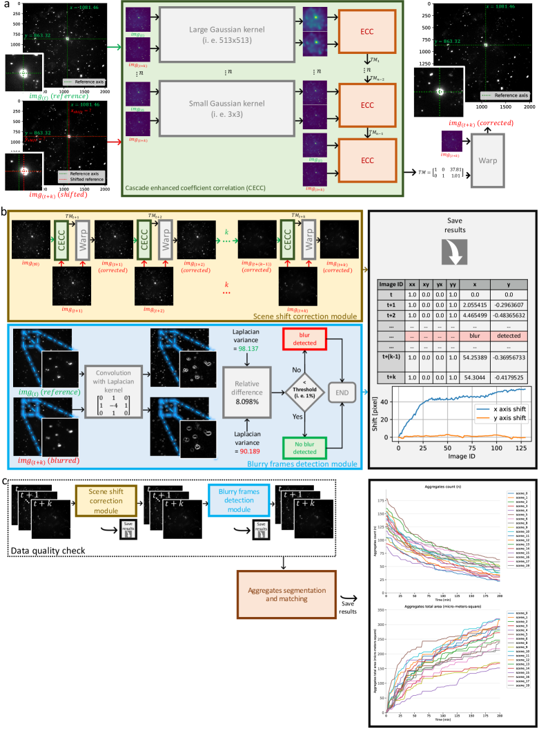
Figure 3: Detailed data quality workflow. (a) Detailed CECC registration approach. (b) Detailed data quality check modules: (i) CECC based scene shift correction module, (ii) blurry frames detection module, and (iii) saving registration information and the rejected blurry frames. (c) Overview of the aggregates quantification workflow: data quality check + segmentation and matching.

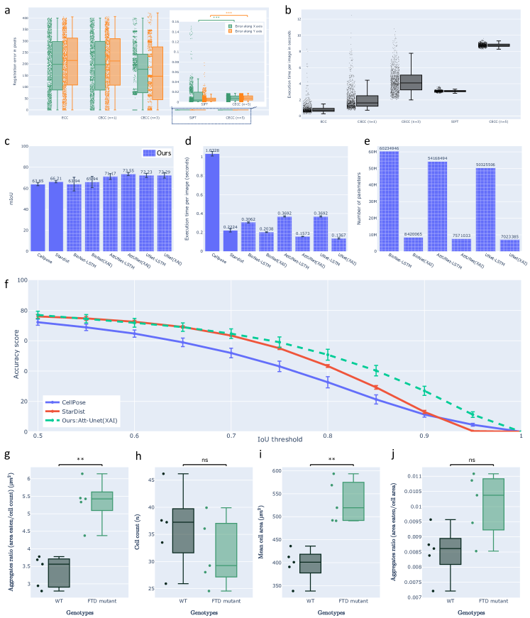
Figure 6: Quantitative performance evaluation of the CECC module, DL/IDL cell instance segmentation module and the phagocytic activity of microglial cells in FTD context. (a) The performance and (b) execution time cost of registration methods ECC, CECC (n=1, 3, 5), and SIFT were evaluated on 1000 randomly shifted frames ($x/y\pm 400px$ shift for $2048^{2}px$ frame). CECC (n=5) achieved the best results with an x/y mean error of $0.008\pm 0.004$, outperforming SIFT. Our cell detection approach was evaluated against Cellpose and Stardist on a 165-image test set, using a 5-fold cross-validation/testing approach to compute (c) mean Intersection over Union (mIoU): sum of IoU of the predicted cell masks divided by the ground-truth cell count; (d) the mean execution time cost per image; (e) number of parameters for DL and IDL approaches; (f) the accuracy $(0.5\geq IoU\geq 1)$ of our best performing approach ’Att-Unet(XAI)’ were computed. Additionally, (g) the amount of TDP-43 aggregates internalized per cell; (h) the number of cells in the assay: cell count; (i) the size of the cells: mean cell area and (j) the amount of TDP-43 internalized per cell surface unit. Statistical tests were conducted using the Mann-Whitney-Wilcoxon test with ns (p-value $\geq$ 0.05), ** (p-value under 0.01), and *** (p-value under 0.001).

Although the application of SIFT proved sufficient in correcting the shift, as demonstrated in Fig. 6.a and in extended data 3 Table.2, we observed a statistically significant directional bias in the shift correction. As a result, we concluded that an unbiased approach was necessary to address the registration problem effectively. To this end, we proposed a generalized version of the Enhanced Correlation Coefficient maximization approach (ECC)[21], which we have termed Cascade ECC (CECC), as illustrated in Fig. 3.a.

CECC offers an unbiased solution, ensuring consistent registration performance irrespective of the shift direction. Our approach achieved sub-pixel precision for shift margins up to $\pm 20\%$ of the image size (i.e., $\pm 400px$ for $2048\times 2048px$ frames). To provide context for these results, the largest unwanted shift observed in our study was approximately 5% of the image size. This demonstrates the robustness of CECC, which offers a 15% margin in the context of the worst-case scenario observed. It is worth noting that there is a significant difference in registration speed between SIFT, with an average of approximately 3 seconds per frame, and CECC (n=5), with an average of approximately 8.7 seconds per frame (refer to Fig. 6.b). This discrepancy can be attributed to the maturity and optimization of SIFT, as compared to the proposed CECC. We anticipate that this gap will eventually be reduced through the contributions of the open-source community.

An other issue worth mentioning when we explored the data is that the microscope lens can get getting out of focus because of physical vibration. This introduce some blurry frames into the scene, which unnaturally amplify the size of aggregates, thus, biasing the phagocytic quantification.

We addressed this issue, by including a blur detection module, that uses image processing to detect the loss of details in images. Then discard them from the stack.

To streamline the data quality check process we combining the CECC-based scene shift correction and the blurry frames detection module (see Fig. 3.b).

This gives the user full traceability over the data quality, making the definition of objective criteria possible. For example, the maximum tolerated shift along either axis x and y can not be more than 50 pixels at any frame, and the maximum tolerated blurry frames in a given scene can not be more than 5%. The data quality check module plays a significant role in detecting (i.e., blurry frames), correcting (i.e., scene shift) and objectively quantifying the severity of hardware/human errors in real-world conditions.

1.1.3 Cellular and aggregates quantification

Cellular quantification: The complex and challenging nature of cell instance segmentation is a significant issue in the field of biological image analysis. This problem involves detecting cells with intricate shapes and diverse morphologies, which has prompted the development of numerous DL-based approaches to address it [12, 22, 23, 15, 16]. While these techniques have proven to be effective, they fail to exploit the temporal information that may be critical for accurately segmenting cells with irregular shapes, such as microglia, which are known for their hyperactivity.

Incorporating spatiotemporal approaches to cell instance segmentation has the potential to greatly improve the accuracy of detection by considering cell movement over multiple frames. This approach can help correct the detected cell masks by introducing time coherency, allowing for a more precise identification of individual cells and their boundaries.

To address these challenges, we propose a generic scheme for robust cell instance segmentation. Our method consists of three primary components: (i) a cell semantic segmentation module, which provides accurate semantic masks for distinguishing cells from the background; (ii) a time-series coherence module that leverages cell movement over time to enhance instance separation; and (iii) a post-processing and refinement step that fuses the instance and semantic information to generate a more accurate representation of cell boundaries.

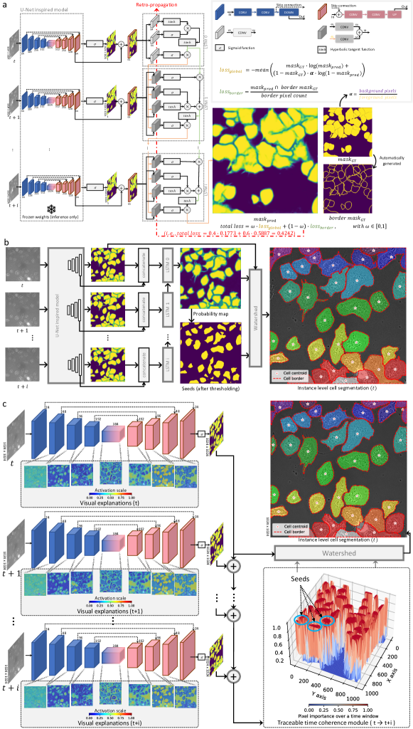
Figure 4: Detailed DL and IDL architectures for cell instance segmentation. (a) Detailed architecture of the segmentation module during the training phase: custom loss functions (global and local) were used during the retro-propagation on the LSTM modules. (b) Detailed inference phase combining U-Net like architectures, LSTM modules and watershed for instance-level cell segmentation. (c) The details of the explainable segmentation module that contains: (i) light U-Net like models attached to a visualization module applied for each time point, (ii) time coherence module (TTCM) that extracts cell seeds, and (iii) watershed module that combines all signals for a full separation.

To substantiate the added value of incorporating temporal information in cell segmentation, we constructed a DL only approach that leverages UNets [12, 24, 25] (UNet, AttUNet and BioNet) as a semantic segmentation module, complemented by the integration of long short-term memory (LSTM)[26] as a time series coherence module (see Fig. 4.a). Furthermore, we utilized post-processing techniques to fuse the previous signals[27, 28], ensuring complete separation between cells (see Fig. 4.b).

As evidenced by Fig. 6.c, our approach, which combines DL and temporal information (AttUNet-LSTM, UNet-LSTM), demonstrates a significant improvement in performance compared to state-of-the-art methods, such as Cellpose and Stardist. However, we observed performance variability when using the BioNet-LSTM (included as a fail case). Upon further investigation, we identified the cause to be rooted in the unique architecture of BioNet-LSTM, which employs an internal recursive mechanism that drastically over-fit the feature maps. This limitation consequently hampers its potential when connected to a time series module, thereby impacting its overall performance. Nonetheless, our findings highlight the importance of incorporating temporal information in cell segmentation approaches to achieve more accurate and reliable outcomes in the analysis of cellular dynamics.

However, the proposed UNets+LSTM approaches, being solely based on DL (DL-only), do not offer interpretability. Despite their superior performance compared to state-of-the-art methods, we consider this lack of interpretability insufficient. We believe that interpretability offers a substantial added value to these approaches. To demonstrate that interpretability does not adversely affect performance, we first initiated the process of "whitening the black box" (i.e., the DL-only approach) to establish that it is not only feasible but also quantitatively comparable to its counterparts (DL-only, Cellpose, and Stardist).

We explored explainable methods [18, 29, 24] and determined that post-hoc feature visualization, represented in the form of heat maps with colors ranging from red for essential features to blue for less critical ones, would serve as a reliable means of gaining insights into the workings of the DL-only approach. This approach would allow for the potential simplification of the process, if deemed necessary, without compromising the effectiveness of the cell segmentation methods.

We generated heat maps for unseen images and attempted to interpret them for all components of the DL-only (UNets+LSTM) approach. Our analysis yielded the following results: for UNets, a substantial amount of unnecessary redundancy in feature maps was observed; LSTM features focused on the less mobile internal parts of cells while utilizing their movement (temporal information) to smooth out cell boundaries for improved separation. From these observations, we concluded that the default number of trainable parameters in UNets was unnecessarily high, and the LSTM effectively harnessed temporal information in a manner that enhanced the overall segmentation process.

Utilizing the DL-only UNets mean feature map as a qualitative reference, we incrementally decreased the number of trainable parameters and halted the process when noticeable qualitative degradation occurred. Despite the simplicity of this intuitive and naive approach, which leaves ample room for improvement, we managed to achieve a 7-fold reduction in the size of UNets (see Fig. 6.e).

Inspired by the LSTM strategy, we devised an image processing-based algorithm called the Traceable Time Coherence Module (TTCM). This algorithm takes into account a time window of cell mask predictions and assigns probabilities ranging from 1 for static cell parts to 0 for moving parts, in a manner that enables cell separation. By incorporating TTCM, we aimed to enhance the overall segmentation process by leveraging temporal information in a similar way to the LSTM approach (refer to Fig. 4.b and Fig. 4c).

The outcome of our efforts was a more compact UNets in comparison to the DL-only baseline. For simplicity, we will refer to these compact versions as UNets(XAI). The visual interpretation-guided optimization was complemented with a visual explanation module to enhance the trustworthiness of UNets. This was achieved by systematically generating heat maps to be presented to biologists and clinicians, illustrating the intermediate steps involved in obtaining the cell mask (refer to Fig. 4.c).

Additionally, the TTCM exhibited unexpectedly advantageous properties compared to the LSTM approach. Notably, it eliminated the need for significant hardware requirements during both training and inference phases, required no training, and provided a flexible time window parameter that can be adjusted as needed—a feature particularly beneficial in research environments. For example, larger time windows can be applied for slow-moving cells, while smaller windows may be more suitable for faster cells.

In terms of performance evaluation, we employed the mean intersection over union (mIoU) metric for each image. This involved comparing the sum of IoU scores of the predicted cell masks with the ground truth masks and subsequently dividing the result by the cell count. This process was carried out for each image in the test set (n=165) using a 5-fold testing approach. The mean and standard deviation were computed for state-of-the-art methods: Cellpose, Stardist, DL-only: Bionet-LSTM, AttUNet-LSTM, UNet-LSTM, and IDL: Bionet(XAI), AttUNet(XAI), UNet(XAI) approaches.

It is important to highlight that in Fig. 6.d, we assessed the inference speed of all considered approaches. For example, Cellpose relies on intensive post-processing to transform vector gradient representation into labeled cell masks, which results in a slower performance compared to other methods.

Additionally, the mIoU metric is well-suited for the comprehensive evaluation of cell detection and segmentation quality without requiring a threshold. However, in the literature [15, 16], average precision (AP) is defined as:
$AP={(TP+TN)}*{(TP+TN+FP+FN)}^{-1}$, with $TN=0$. We contend that this metric is, in fact, the accuracy metric, which differs from the standard AP metric employed in object detection problems, defined as the area under the precision/recall curve. Indeed, accuracy has been used in previous studies [15, 16] to evaluate detection quality.

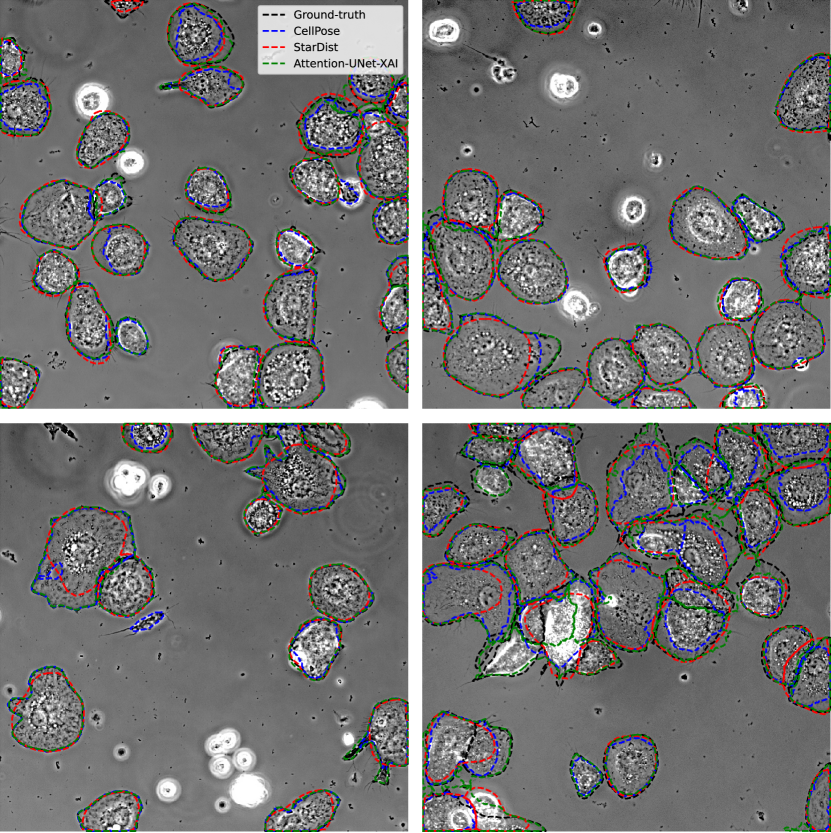
Figure 9: Instance-level cell segmentation evaluation: Our qualitative analysis demonstrates that the Attention-UNet(XAI) model performs favorably in comparison to Cellpose and Stardist, particularly in handling challenging cell shapes. This evidence suggests that our approach adapts effectively to the complexities associated with cell morphology, showcasing its potential to provide a competitive alternative to existing state-of-the-art methods. Notably, in extreme cases where cells are agglomerated and still in suspension (as seen in the white cluster of cells at the bottom right), all methods, including our own, struggle to achieve accurate segmentation. Such instances highlight the need for further refinement and optimization to address these challenging scenarios effectively.

To maintain continuity with the metrics previously used in Cellpose [16] and Stardist [15], we included Fig.6.f, where we applied the same accuracy metric to compare our best-performing mIoU approach – ’AttUNet(XAI)’ – with state-of-the-art methods. We utilized different IoU thresholds and computed the mean and standard deviation values over 5-fold cross-validation and testing. Our method significantly outperforms both Stardist and Cellpose when $IoU>0.8$. This result demonstrates that our approach is well-suited for fast, efficient, and high-quality instance-level cell segmentation. For a quantitative/qualitative comparison, please refer to the extended data3: Tab.2 and Fig.9.

It is worth mentioning that we employed the default configurations of state-of-the-art methods (Cellpose and Stardist) [15, 16] as described in their respective publications, utilizing their provided source code. We observed a longer training time for these methods compared to our DL-only and IDL approaches. Specifically, Cellpose requires 500 epochs, and Stardist necessitates 400 epochs, while our IDL approach takes only 20 epochs, and the DL-only method takes 40 epochs. This observation highlights the efficiency of our proposed methods in terms of training time.

The key takeaways from our results are as follows:

• Fig. 6.c demonstrates that incorporating temporal information significantly enhances the performance of segmentation methods, and interpretability can be achieved without sacrificing performance.

• Fig.6.d and Fig.6.e confirm that interpretability offers valuable optimization properties, such as improved processing speed and reduced hardware requirements.

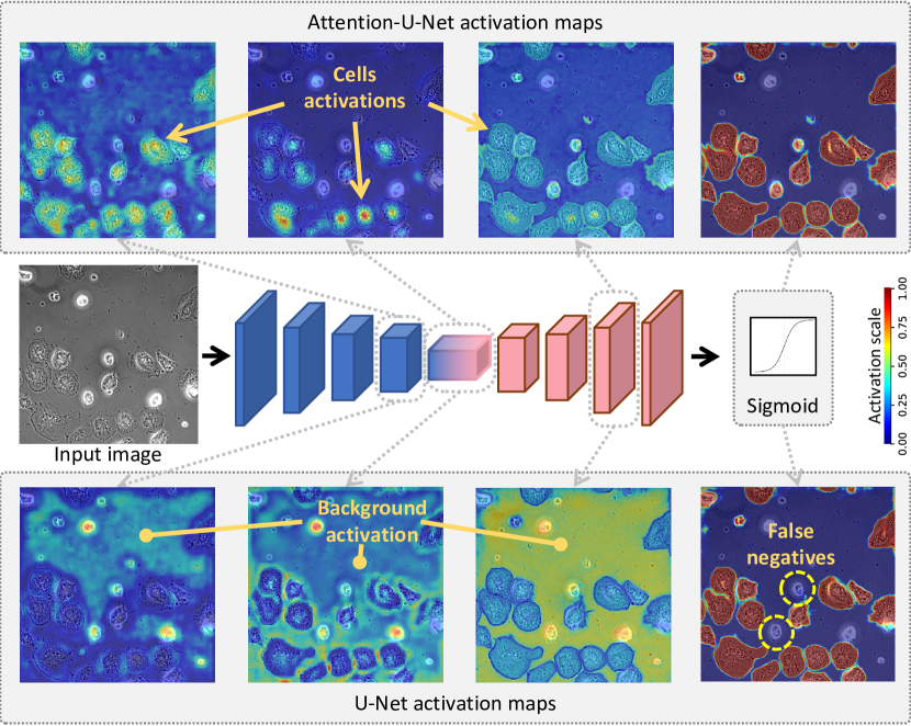
Figure 7: Visualization of the features learned by U-Net versus Attention-U-Net. U-Net model focused more on the background features since the background texture is easier to model compared to the texture of the cells. Consequently, it led U-Net to produce false negatives. On the other hand, Attention-U-Net uses the attention mechanism, which makes it focus on the cells’ texture, thus, yielding fewer false negatives compared to U-Net.

Some unexpected results emerged when we applied feature visualization to UNet and AttUNet in the context of cell segmentation. The UNet model employs an encoder to extract background features, focusing on the mid-section ’bottleneck’ of the model. Subsequently, the decoder disregards the background and utilizes skip connections to generate segmentation masks. This observation can be attributed to the relative complexity of modeling foreground texture, which exhibits a high degree of variation, as opposed to the uniform background. By interpreting the heat maps, we confirmed that UNet adopts a less demanding approach, concentrating on background feature extraction and then estimating the complementary mask to produce cell masks. In contrast, the AttUNet model incorporates an attention mechanism [30, 24] in addition to the UNet structure. Feature visualizations revealed that the attention mechanism actively alters the learning behavior of the model (compared to UNet), directing its focus more towards cell features, unlike the UNet model. Interestingly, even when trained on the same dataset, UNet and AttUNet models can tackle the same task and achieve comparable segmentation performance while learning distinct sets of features (see extended data 3: Fig. 7).

Aggregates quantification: In order to accurately detect and quantify aggregates in time-lapse videos, we developed a specialized module that processes data through a series of steps. In summary, these steps include: (i) applying a threshold-based segmentation tailored for fluorescent aggregates; (ii) labeling the binary mask to separate individual aggregates; (iii) computing and saving the count, surface area, and coordinates of aggregates; and (iv) quantifying phagocytized aggregates based on changes in surface area and coordinates. Upon testing, we determined that utilizing the change in surface area of aggregates effectively captures two critical aspects: the surface area reduction when a cell begins internalizing an aggregate in a bite-by-bite manner, and the change in coordinates when the aggregate becomes small enough to be moved and internalized by the cell. By combining these two criteria, we can appropriately quantify phagocytosis, as when a given aggregate is fully internalized by a cell, it is considered to be phagocytized.

In our study, we utilized fluorescent aggregates, where high pixel intensities indicate the presence of an aggregate and low pixel intensities signify its absence. Consequently, a simple threshold was sufficient to accurately segment the aggregates. Furthermore, our experimental setup ensures that aggregates are initially fixed in the presence of cells. This implies that if the aggregates move, it is due to cellular activity. Therefore, tracking aggregate movements involves monitoring the changes in the aggregate centroid compared to its initial position through image processing. It is important to note that this approach may not be effective if one of the assumptions, such as initial aggregate fixation or fluorescence, is not met.

1.1.4 Spatiotemporal superposition/analysis of aggregates and cells for phagocytosis quantification

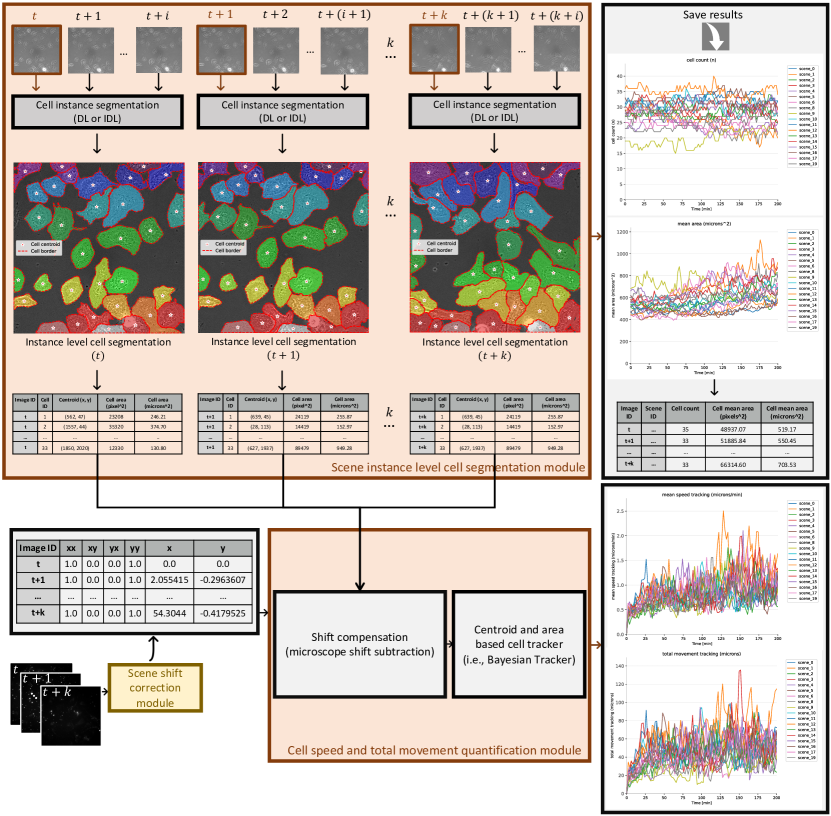
Figure 5: Scene cell instance segmentation and tracking. The scene instance-level segmentation module can use the DL module (Fig.4.b) or the IDL module (Fig.4.c) for a scene cell instance segmentation. This module quantifies cell count, area and coordinates for each frame. Cell speed and total movement quantification loads the scene cell features (frame id, centroid, area). Cell centroids are corrected using scene shift correction module (Fig.3.b). For cell speed and total movement quantification, any tracking algorithm (i.e., Bayesian Tracker) can be applied on the corrected cell features. Results of all complementary modules are saved in an open-source format (i.e., CSV).

To summarize the various modules of the presented pipeline, ’PhagoStat’, which is dedicated to phagocytosis quantification (refer to Fig.1): initially, computational resources are automatically allocated in the case of computation on a cluster (see Fig.2.b); otherwise, a local machine is employed. The raw data is loaded, normalized, and separated into two channels for cells and aggregates (see Fig.2.a). The aggregate data is utilized to correct any detected shift and remove blurry frames from the stack, if present (see Fig.3.b). Subsequently, the aggregates are segmented, and their morphological features (i.e., area, count) are quantified (see Fig.3.c). The cell data is processed through the scene instance-level cell segmentation module (see Fig.5) to extract cell area and coordinates. These features are then used to track cells and estimate cell speed and total movement[31, 32]. Additionally, heat map visualizations and traceable time coherence data are provided (see Fig. 4.c), resulting in a fully interpretable pipeline.

All the results are compiled and organized by condition to generate a comprehensive statistical report. It should be noted that, currently, the statistical reporting is limited to only two conditions. Therefore, in cases where more than two conditions are being used, the reporting framework would need to be adapted accordingly to accommodate the additional conditions.

To provide a sense of the efficiency of our pipeline, it takes approximately 20-30 minutes to process raw data and generate the final statistical report. This processing time applies to 20 scenes, each lasting for 7 hours, with aggregate and cell frame pairs captured every 2 minutes. The pipeline’s performance was evaluated using a high-performance computing cluster equipped with only Central Processing Units (CPUs). It is expected that the processing time could be further reduced if Graphics Processing Units (GPUs) were utilized, highlighting the pipeline’s potential for rapid and effective analysis.

1.2 Microglial cells phagocytosis use case

The dual role of microglial phagocytosis, encompassing aggregate clearance and the abnormal phagocytosis of live neurons and synapses, has been a topic of investigation for several years in various neurodegenerative diseases, such as Alzheimer’s and Parkinson’s diseases [4, 5, 6, 7, 8]. In order to establish our assay, we focused on the case of FTD mutations, where the two most frequently mutated genes in familial forms of the disease – C9ORF72 and GRN – are highly expressed in microglia and are believed to regulate microglial functions, particularly phagocytosis [33, 34, 35]. Given that TDP-43 aggregates accumulate in the degenerating neurons of patients [36, 37], aggregate clearance is anticipated to yield positive therapeutic outcomes. Conversely, excessive synaptic pruning or phagocytosis of live neurons could exacerbate degeneration. This has been demonstrated in the case of C9ORF72, where mutations involved in neurodegenerative diseases can influence both opposing effects [34].

Moreover, numerous simple phagocytosis assays exist, utilizing latex beads or pH-sensitive fluorescent particles. Nonetheless, the development of sensitive assays capable of analyzing phagocytosis using physiological targets, such as protein aggregates and functional neuronal networks, and breaking down microglial phagocytic behavior is of significant interest. This approach is crucial for the development and screening of therapeutic compounds aimed at targeting abnormal phagocytic activities.

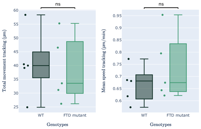
Figure 8: Additional quantitative results of FTD-mutant versus WT microglial cells. (right) the quantification of total cells movement. (left) the quantification of the cells’ mean speed. (statistical test: Mann–Whitney–Wilcoxon, ns: p-value $\geq$ 0.05)

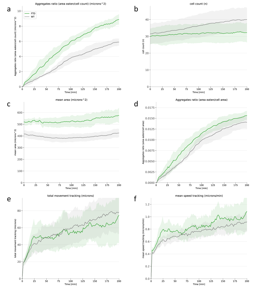
Figure 10: Comparative analysis of phagocytosis metrics over time for WT and FTD Groups. This figure presents a time-course comparison of phagocytosis-related parameters between WT and FTD groups. The panels display (a) aggregate area consumed by cells, (b) cell count, (c) mean cell area, (d) cell surface area consumption, (e) total cell movement, and (f) cell speed over time. This analysis highlights the dynamic differences in phagocytosis between the two conditions and enables a comprehensive understanding of their distinct behaviors.

In an effort to estimate the on-target phagocytic activity of WT and FTD-mutant microglial cells, we analyzed the amount of TDP-43 aggregates internalized per cell (Fig. 6.g: aggregates ratio = area eaten/cell count). Interestingly, FTD mutant cells seem to display increased phagocytosis of TDP-43 aggregates, with FTD mutants being approximately 70% more aggressive than their WT counterparts. We ensured that the number of cells in the assay (Fig.6.h: cell count) was similar, yet we observed that the size of the cells was significantly larger in FTD-mutant microglial cells (Fig.6.i: mean cell area). Notably, FTD mutants were approximately 30% larger than WT cells, a finding that, to our knowledge, has not been proven before. As a result, we measured the amount of TDP-43 internalized per cell surface unit (Fig. 6.j: aggregates ratio = area eaten/cell area) and found that a portion of the increased phagocytic activity of FTD-mutant microglial cells could be explained by the increased spreading of the cells. Moreover, no global modification of the total quantity of movements or the speed of the movements of the cells was observed in this case (refer to extended data 3: Fig. 8 and Fig.10).

1.3 Phagocytosis dataset for microglial cell

In this study, we have chosen to analyze the phagocytosis of protein aggregates by microglia in the context of frontotemporal dementia (FTD). FTD is a neurodegenerative disease in which mutations in genes regulating microglial functions (such as C9ORF72 and GRN) correlate with a specific type of aggregates composed of the TDP-43 protein [38, 36, 37]. Since the distinction between C9ORF72 or GRN is not pertinent to the scope of this work, we will refer to FTD mutants for simplicity.

The data acquired for this study consists of acquisitions from wild-type (WT, n=5) and frontotemporal dementia (FTD, n=5) microglial cells during the phagocytosis process. Each acquisition captured 20 distinct scenes, encompassing seven hours of time-lapse video microscopy (recorded at one frame every two minutes). Cell and aggregate images were collected in two separate channels.

Our dedicated team of biologists has meticulously generated a comprehensive dataset, which has been subjected to rigorous validation by the laboratory’s ethical committee. This dataset encompasses 36496 normalized cell and 36496 aggregate images, accompanied by 1306131 individual instance masks for cells and 1553036 for aggregates, 36496 registered aggregates and data of the intermediate steps in tabular format all generated using the PhagoStat algorithm. To ensure the highest quality of data, we have applied data quality correction techniques.

The dataset provides an extensive array of biological features, such as area, position, and speed, which are presented in a frame-by-frame manner to allow for in-depth analysis. Moreover, to enhance the dataset’s value, we have incorporated 226 manually annotated images containing 6,430 individual cell masks. These images were randomly selected from different conditions, including wild-type (WT) and frontotemporal dementia (FTD), and were obtained from a diverse range of randomly chosen scenes.

The result is a robust dataset comprising a total of 235288 files (94GB), offering researchers a valuable resource for investigating various cellular and aggregate properties in their studies. By providing such a comprehensive dataset, we aim to advance our understanding of cellular dynamics and contribute to the development of novel therapeutic strategies for conditions like frontotemporal dementia.

Through the release of this valuable dataset to the scientific community, our primary objective is to foster a deeper understanding of the underlying methodologies and to facilitate the wider application of our established pipeline. This initiative is designed to propel advancements in research across the fields of bioinformatics, computational modeling, and cellular biology. By doing so, we aim to encourage innovation and collaboration among researchers working in these interconnected disciplines.

Discussion

Phagocytosis is a vital cellular process that serves as a primary defense mechanism against danger signals and pathogens, ensuring the proper functioning of the immune system. In the brain, microglial cells are the sole cell type capable of performing phagocytosis. The phagocytic activity of these cells has garnered increasing attention in the study of neurodegenerative diseases, as neuroinflammation appears to play a significant role in the pathological processes. This role may involve the clearance of aggregate formations or the abnormal phagocytosis of live neurons and synapses by microglia. Furthermore, antibody-mediated clearance of aggregates by phagocytic microglia is currently being explored as a therapeutic strategy for Alzheimer’s disease and other forms of dementia.

Quantifying the phagocytosis of amorphous and highly active unstained cells is a challenging task, which is essential for investigating a wide range of neurodegenerative diseases. This task often involves phase-contrast time-lapse video microscopy to observe rapid interactions between cells, making it difficult to distinguish the cells of interest from the background.

In response to the challenges associated with quantifying microglial cell phagocytosis, we have developed PhagoStat, a fully automated, real-time, scalable, open-source pipeline specifically tailored for high-content video microscopy instance segmentation and tracking. PhagoStat has been meticulously designed and rigorously tested, with a focus on interpretability and explainable artificial intelligence, ensuring that it offers capabilities comparable to state-of-the-art methods.

This innovative design enables scientists to trust, understand, and utilize individual modules for specific needs or to employ the entire pipeline in the context of time-lapse image analysis. Furthermore, PhagoStat offers essential genericity and reproducibility, which are critical components of reproducible science. This not only facilitates compliance with the General Data Protection Regulation (GDPR) but also promotes faster and more effective translational adoption.

By providing an interpretable and transparent pipeline, PhagoStat empowers experts and users, such as laboratory technicians, biologists, physicians, and supervisors, to gain a deeper understanding of the studied processes. Additionally, this approach opens up exciting possibilities for pipeline design optimization tailored to specific use cases. As modern technologies increasingly demand a lower carbon footprint, PhagoStat offers valuable insights into the design of individual modules, ensuring that the pipeline remains both efficient and environmentally responsible.

Effective data quality check capabilities are essential for adapting to real-world acquisition conditions in scientific research. One limitation of our current approach, however, is the need for optimization improvements in our registration method, the CECC, which takes longer than the widely-used SIFT method. It is crucial to further investigate the bias detected when using the SIFT method, as this may offer valuable insights for enhancing our pipeline.

Our analysis suggests that the bias observed in the SIFT method could be related to issues with landmark identification. We believe that this issue may arise from at least one of the following reasons: 1) an insufficient number of landmarks, as the signal is predominantly background, or 2) indistinguishable landmark features due to the geometric similarity of aggregates. Eventhoth our CECC method appears to be immune to these issues, it comes at the expense of speed. It is essential to further investigate these potential causes to ensure the robustness and accuracy of our pipeline, especially if SIFT is considered as an alternative to CECC for faster results.

Although transitioning from a DL-only to an IDL naive approach has led to a seven-fold reduction in model size across the board, there is still room for improvement. Automating the assessment of feature map degradation with an objective metric and a proper methodology could help select smaller models, save time for experts and machines, and remove human subjectivity from the optimization process, thereby promoting a more universally applicable scientific criterion.

Despite the promising properties of the TTCM described in this work, TTCM relies heavily on the UNet predictions at different time points. This will yield good results only if UNet-like models are well-performing on the test distribution. One possible direction for improvement could involve the full integration of TTCM into the UNet during training, supplemented by a time coherence loss function.

In this study, we employed FTD-mutants and WT cells as a use case to demonstrate the utility of our pipeline. For the sake of simplicity, we grouped GRN and C9ORF72 mutations together as FTD-mutants. It is important to note that there may be biological differences between GRN and C9ORF72 mutations, which are beyond the scope of this work. The investigation of these differences should be addressed in future studies, in order to enhance our understanding of the specific characteristics and implications associated with each mutation type. By elucidating these distinctions, researchers can potentially develop more targeted and effective therapeutic strategies for neurodegenerative diseases involving these mutations.

Addressing these limitations and investigating the underlying reasons could further enhance the pipeline’s reliability and efficiency for scientists working in the field of microglial cell phagocytosis.

Finally, to support community efforts towards a better understanding of neurodegenerative diseases, we are releasing the pipeline as open-source and unveiling a unique, massive microglial cell phagocytosis dataset. This milestone dataset serves as a first reference benchmark, stimulating the emergence and consolidation of algorithms dedicated to this critical domain and contributing to high-content biomedical image analysis in general.

Methods

Data efficient loading and normalization. Most of the proprietary microscope software (biologists friendly) are working exclusively on Windows. Therefore, data preparation required specific steps: (i) raw data was first transferred from the microscope machine to a Windows machine; (ii) the acquisition was converted into tagged image file format (TIFF) frames; (iii) the frames were arranged to be compatible with the computational pipeline and iv) the resulting frames were transferred to a high performance computing (HPC) cluster for processing. A notable challenge in this process was the lack of transparency we found when running the software’s preprocessing (black-box) steps (i.e., normalization, the conversion of the raw data 16bit to TIFF 8bit frames). Besides, the rich and user-friendly visualization interface, such packages turned out to be overly opaque, inefficient, resource-intensive and time-consuming for analyzing big data. To overcome these drawbacks, we have adapted the ’aicspylibczi’[39] to develop a flexible, robust, and open-source module capable of reading and converting proprietary raw data formats into universal image formats. Our module was tested on converting Carl Zeiss Image (CZI) files to TIFF format, and it is compatible with Windows, macOS, and Unix. Additionally, the module can be easily adapted to take advantage of HPC clusters and parallelization schemes (refer to Fig.2.a and Fig.2.b).

The ’aicspylibczi’[39] Python package was used and extended to read the ’CZI’ raw data file using delayed reading. This approach allowed us to read cell and aggregate channels image-wise without loading all the sequences to the RAM. Images were in 16bit representation. Frame reading time can be accelerated by coupling the Python package with multiple CPUs for parallel processing. This involves several scenes being simultaneously read, with each scene being allocated to its own CPU. This deviates from sequential processing, in which scenes are placed in a queue and read sequentially; (i) in the local machine, our package can use multi-CPUs for parallelism, or (ii) in a HPC clusters that use simple linux utility for resource Management (SLURM), where our package launches an array of jobs (i.e., attributing to each scene a job ID) on the same node or different nodes.

While using the same parallelism scheme, global percentile normalization is used to re-scale the image pixels’ intensities of the whole sequence; 0.5% and 99.5% percentiles for aggregates; 0%, 100% for cells. Aggregate and cell images were re-scaled from 16bit to 8bit using ’img_as_ubyte’ function from the ’scikit-image’[40] Python package. Histogram matching with a normal pixel distribution as reference is used on all cell images, and we apply it using the ’match_histograms’ function from the ’scikit-image’ Python package. Finally, if needed, images were resized from $2048\times 2048$ to $1024\times 1024$, then saved in ’TIF’ format using the ’PIL’ Python package.

Quantitative performance evaluation of the readout module. The proprietary Carl Zeiss Microscopy ZEN light v3.3.89.00 software was used as a reference for data loading and saving. This proprietary software was evaluated using a Windows 11 machine with 8 cores i7 9700K CPU, 16GB RAM, Nvidia RTX2080 GPU and Samsung 970 PRO SSD; all drivers were up-to-date. CUDA acceleration was enabled from the software configuration panel; all parameters were left at their default values, and no tasks ran in the background before/during the benchmark.

Our approach uses only open-source Python packages, as described and cited before. Ubuntu 20.04LTS was used with: 8 cores, i7 9700K CPU, 16GB RAM, HDD or SSD. For single-CPU tests, the hardware used was limited to 1 CPU using ’taskset’. The test was monitored, and during the test, RAM usage did not exceed 1GB (while using an HDD or SSD). For the multi-CPU test, SLURM was used to process 20 job arrays. Each one uses 1 core Xeon Gold 6126 CPU and 1GB RAM (while using HDD or SSD storage node).

All data transfers (single raw data file or frames) were performed using a 1GB/s Ethernet port with ’FileZilla’ v3.46.3. SFTP transfer protocol was used while directly connected to the internal institute network (no VPN used); maximum simultaneous transfers were set to 10 files (FileZilla’s upper bond).

Frame registration and correction. We applied SIFT [20] algorithm to two frames affected by the shift problem. First, we identified the main points of interest and cross-referenced them with the next frame. Then, the outliers were discarded to estimate the transformation matrix, thereby canceling the shift. However, according to our performance evaluation, SIFT was sufficient to correct the shift (see Fig. 6.a also in extended data 3 Table.2). Finally, it obtained an average error of $0.0153\pm 0.0609px$ along the x-axis, while $0.0228\pm 0.1221px$ along the y-axis. Thus, SIFT proved to be directionally biased by the shift. SIFT was tested using the ’SIFT_create’ function from the ’OpenCV’[41] library to compute key points and their source and target image descriptors. The Euclidean distance (default sift error=0.7) matches points between the two key-points descriptors. The random sample consensus (RANSAC) algorithm eliminates outliers (the ’RANSACRegressor’ function from the ’scikit-learn’ library). The matched points are used to find the transformation matrix.

Our recursive scheme (in our CECC module) considers the peculiarities and challenges of this registration task. First, we used a relatively large Gaussian kernel (i.e., 513) to preserve the essential details of the aggregates while reducing noise. Then, we estimated an initial transformation matrix $TM_{0}$ to compensate for the offset between consecutive frames. Next, we applied a smaller Gaussian kernel (i.e., 257) to add more aggregate detail and initialized a second registration process using $TM_{0}$, resulting in $TM_{1}$, which compensated more efficiently for the acquisition shift. We repeated this step-wise process N times, decreasing the kernel size at each step until no kernel was applied, estimating $TM_{N}$ using ECCM directly on the original frames and using $TM_{N-1}$ as an initialization.

To implement the CECC approach, we used the ECC implemented in the ’OpenCV’ v4.5.1 Python library named ’findTransformECC’. Each cascade used a different Gaussian kernel, with 1000 max iterations or $10^{-4}$ error as a termination criterion for finding the corresponding transformation matrix. The last cascade computed the effective transformation matrix.

When the transformation matrix is estimated, the ’warpAffine’ function (from the ’OpenCV’ library) is used to register the image by the computed transformation matrix.

In order to validate our registration approach, 1000 ’x’ and ’y’ shifts were randomly generated and then saved between -400 pixels and 400 pixels (x and y shifts are independent). For each test, we loaded the reference image (containing aggregates) and the same random shifts, in the exact same order. We created a shifted version of the reference image using ’warpAffine’, with the loaded shifted ’x’ and ’y’. Both images (reference and shifted) are $2048\times 2048$ gray-scale. Each test was submitted as a job via SLURM to a computational cluster. For CECC, we used 4 cores Xeon Gold 6126 CPU, 1GB RAM and for SIFT 4 cores Xeon Gold 6126 CPU, 2GB RAM (1GB RAM for SIFT is not sufficient). The execution time is computed and reported for each registered image.

For blurry frame detection module, we computed the Laplacian of two images: image(t) and image(t+k), where k is the step between two images (i.e., k=1 means comparing two consecutive images). Then, the module evaluate the variance of the resulting images. Images with no blur give high variance values, and images with blur give low variance values. This mechanism effectively detects sudden drops in Laplacian variance values (using the relative difference compared to a given threshold), thus detecting blurry and unusable frames (i.e. dropped from the stack).

In order to compute the Laplacian image we used the ’Laplacian’ function from the ’OpenCV’ Python library in 64 float representation. Variance is then computed on the resulting image. Every two consecutive frames, the relative difference is computed, and the blurriness is detected if:

$$\lvert 1-\frac{\sigma^{2}(\nabla^{2}_{5}f_{t+1})}{\sigma^{2}(\nabla^{2}_{5}f_{t})}\rvert>\varepsilon_{blur},\leavevmode\nobreak\ where\leavevmode\nobreak\ \varepsilon_{blur}\in[0,1]$$ (1)

with $\sigma^{2}$ the statistical variance and $\nabla^{2}_{5}$ the five point operator [42]. If the blur is detected (i.e., $\varepsilon_{blur}=0.01$), a loop is launched to check for the disappearance of the fuzziness in the next $B$ frames (i.e., $B=14$).

When faced with long episodes of blur (many consecutive fuzzy frames), a bigger $B$ value is recommended. However, one usually look for low $\varepsilon_{blur}$ values, corresponding to a higher quality standards. This module record and save all the shift correction parameters as the rejected blurry frames.

Aggregate segmentation and quantification. After aggregate image normalization and data check, we used a fixed 0.5 threshold to separate the aggregates from the background. Next, we labeled the segmented aggregates to extract features (i.e., count, area and centroid) using the ’label’ and ’regionprops’ functions from the ’scikit-image’ library. To consider that a given labeled aggregate is phagocytosed by a cell, we checked every two consecutive frames if the following conditions are met: the change in the size of the labeled aggregate (decrease by half) and its centroid movement ($0.7\mu m$ $\approx$ $7\leavevmode\nobreak\ pixels$). Finally, all aggregates’ features for each time point are reported/saved.

Scene instance-level cell segmentation and tracking modules.

DL and IDL approaches: U-Nets used four depth levels. In the down-sampling pass, for U-Net and Attention-U-Net, each depth level had a duplication of the following sequence: 2D convolution layers (Conv2D) with 3x3 filters, 2D batch-normalization and leakyReLU, then, 2-factor max-pooling. BiO-Net used a duplication of the following sequence: Conv2D, 2D batch-normalization and ReLU. This sequence is followed by Conv2D, ReLU, 2D batch-normalization and 2-factor max-pooling. The results of each depth level are connected to the symmetrical depth of the decoder as ’skip’ connections.

The midsection (bottleneck) for U-Net and Attention-U-Net was composed of a duplication of the sequence: Conv2D, 2D batch-normalization, leakyReLU. The BiO-Net bottleneck was composed of Conv2D, ReLU, 2D batch-normalization, Conv2D, ReLU, 2D batch-normalization, 2D transposed convolution, ReLU, 2D batch-normalization.

In the up-sampling pass, each depth level used up-sampling with a scale factor of two, and then the skip connection is concatenated differently for each model. In U-Net, it is directly concatenated along the first dimension with two times: Conv2D, 2D batch-normalization and leakyReLU. The Attention-U-Net passed the up-sampled signal through: Conv2D, batch-normalization, and leakyReLU. Then, the attention module (see details [24]) processes the resulting signal and the skip connection. This result is concatenated with the skip connection along the first dimension and passed through the sequence: Conv2D, 2D batch-normalization and leakyReLU. The BiO-Net used the same U-Net decoder module, by only replacing leakyReLU with ReLU. In addition, batch-normalization comes after the ReLU activation function.

For all U-Nets, the output was a single channel image (after Conv2D followed by a sigmoid function). We used the same 2D convolution layers for the encoder and decoder. DL U-Nets contains a (64, 128, 256, 512) sequence of layers for each depth level with a midsection of 1024 layers. IDL U-Nets involved (24, 48, 96, 192) series of layers for each depth level and a midsection of 384 layers. For the BiO-Net, the default 1 iteration and a multiplier of 1.0 are used.

LSTM modules (described in Fig.4.a) were connected to the frozen U-Nets (forward-pass only). The highest encoder depth convolution results (64x1024x1024) were concatenated with the prediction image (1x1024x1024) and passed to the $LSTM_{0}$ when the given frame is the first one in the chosen time-window (successions of frames), otherwise to $LSTM_{i}$.

The TTCM (presented in Fig.4.c) concatenated the probability maps from U-Nets. These results were then normalized by the number of the time points. Seeds were finally extracted using a high thresholding (i.e., 0.9), corresponding to selecting the pixels presented in most of the frames of the time-window.

The visual explanation module is connected to the XAI U-Nets. Each depth level (encoder and decoder) output was extracted before the mean activation heat map was computed along axis 1. The resulting image was scaled to match the input image dimensions (1024x1024) using the ’resize’ function from the ’PIL’ Python library.

DL training phase: U-Nets were trained for semantic segmentation: background and foreground separation. We designed a binary cross entropy-based loss function to address the unbalance background/foreground pixel count. By considering the pixel count for each training image to adjust the loss function systematically. For instance, when a given image $i$ has a low cellular density, the loss function gives more importance to the cell pixel class. The global loss is, therefore, defined as:

$$loss_{global}=-\frac{1}{I}\sum_{i=1}^{I}\left[gt_{i}\cdot log(pred_{i})+(1-gt_{i})\cdot\alpha_{i}\cdot log(1-pred_{i})\right]$$ (2)

With $\alpha$ is the ratio between the number of background and foreground pixels from the ground truth, $I$ represents the number of training images, $gt_{i}$ the ground truth binary mask, $pred_{i}$ the model prediction. In order to optimise the speed, the ’PyTorch’ library is used to flatten the masks. Then the loss function is computed directly on the GPU, by significantly reducing the delay between the forward and the backward passes.

In a first phase of the DL training, all U-Nets were trained using 5-fold cross-validation and testing while using: (i) $loss_{global}$ for retro-propagation (see equation 2); (ii) Adam optimizer; (iii) $10^{-4}$ learning rate and (iv) batch size of one. After twenty epochs, the best model was saved for each validation fold based on its $loss_{global}$ score on the validation set, then tested on the test set. In order to take into account the cell border and to reduce the training time, border masks were automatically generated for the dataset in the following manner: cell binary mask was dilated using the ’binary_dilation’ function from the ’scipy’ library for two iterations, the pixels of the original mask was subtracted (keeping only the borders after dilation), then the border mask was dilated for 4 successive iterations (see Fig.4.a). We defined the border loss as:

$$loss_{border}=\frac{1}{I}\sum_{i=1}^{I}\frac{pred_{i}\cap gt\_border_{i}}{\sum_{p=1}^{P}gt\_border_{i,p}}$$ (3)

With $I$ the number of training images, $gt\_border_{i}$ the automatically generated ground-truth border binary mask, $P$ the number of pixels for a given border binary mask and $pred_{i}$ the model prediction. When the model prediction entirely separates the cells, the $loss_{border}=0$. On the other hand, if the prediction totally overlaps with the dilated borders, $loss_{border}=1$.

In a second phase of the DL training, the parameters of the U-Nets were frozen (no back-propagation). Then, the U-Nets were connected to LSTM modules with two-time point window at a time ($LSTM_{0}$ and $LSTM_{1}$). This allowed back-propagation to only change LSTM parameters (see Fig.4.a). In our training, the loss function was a combination of equations 2 and 3:

$$total\_loss=\omega\cdot loss_{global}+(1-\omega)\cdot loss_{border},\leavevmode\nobreak\ \leavevmode\nobreak\ \leavevmode\nobreak\ \omega\in[0,1]$$ (4)

In order to give more importance to cell borders, $\omega=0.4$ was used, thus, improving the separation of the cells. LSTM modules were trained using the 5-fold cross-validated U-Net frozen models, $total\_loss$ with $\omega=0.4$ (see equation 4), Adam optimizer, $10^{-4}$ learning rate and a batch size of one. After twenty epochs, the best model was saved for each validation fold based on its $total\leavevmode\nobreak\ loss$ score on the validation set and then tested on the test set.

IDL training phase: U-Nets were trained using 5-fold cross-validation and testing, $loss_{global}$ for retro-propagation (see equation 2), Adam optimizer, $10^{-4}$ learning rate, batch size of one. After twenty epochs, the best model was saved for each validation fold based on its $loss_{global}$ score on the validation set, then tested on the test set.

DL/IDL inference phase: For DL we used UNets+LSTM and for IDL we used UNets+TTCM. These modules combination produced time-series-based probability maps (high-values: cells, low-values: background and cell borders). Then, cell seeds (centroid coordinates) were extracted after 0.9 thresholding. Watershed method combined the probability map as a distance map, cell centroids as seeds and the binary mask (U-Nets predictions after 0.5 thresholding) as a foreground delimiter (see Fig.4.b, Fig.4.c). Moreover, the execution time evaluation (during inference) presented in Fig.6.d was performed using the following hardware 8 cores i7 9700K CPU, 16GB RAM, Nvidia RTX2080 GPU and Samsung 970 PRO SSD.

Cell tracking: The Bayesian Tracker (btrack)[31, 32] Python library was used to track cells over time. It used the centroid and area to form cell tracks. Only the tracks with at least 100 min long were kept. Speed was computed at each time point (mean cell displacement divided by time unit), quantifying speed over time, and then, mean speed over a whole sequence was computed and reported. A similar approach was used to compute total displacement over time and for the whole sequence.

Microglia primary culture. Microglia primary cultures were performed using newborn brains of controls (C57BL6/J), of FTD-mutant animals (line C9orf72-/- or GrnR493X/R493X). Newborn mice brains (less than two days old) are collected by dissection of the skull. Brains are recovered in a 50mL Falcon and mechanically dissociated by gentle pipetting into 5mL of Hank’s Balanced Salt Solution (HBSS Thermo Fisher Scientific 14025050). After dissociation, the resulting cell suspension is then centrifuged at 1200rpm for 10 minutes at 4°C. The pellet is re-suspended with culture medium containing DMEM (Thermo Fisher Scientific 31885023), supplemented with 10% de-complemented calf fetal serum free of endotoxins (HI FBS Thermo Fisher Scientific 10082147), 1% Penicillin + Streptomycin (Thermo Fisher Scientific 15070063). The cell suspension is cultured in flasks (75 mm2) previously coated with Poly-L-Lysine (SIGMA P4832) for 30 minutes at 37°C (5% CO2) then washed three times with 1X Phosphate Buffered Saline. The culture flasks are incubated at 37°C (5% CO2). Fifteen days later, microglia are ready for harvest. Microglia are obtained by light shaking and recovery of the culture medium in a 50mL Falcon. After centrifugation, cells are re-suspended in fresh culture medium and plated.

Phagocytosis assay. Aggregates of recombinant human full length TAR DNA-binding protein 43 (TDP-43, Abcam ab156345) were conjugated to Alexa Fluor 555 NHS Ester (ester succinimidyle, Thermo Fisher Scientific A20009) at equimolar concentration and deposited on a 35 mm glass-bottom dish (Ibidi, 81218-200) for 2 hours at $37^{\circ}$C, 5% CO2. The dish was then washed 3 times with 1X phosphate buffered saline (PBS) and $12.5$ x $10^{5}$ freshly harvested primary mouse microglia (WT, Grn KO or C9orf72 KO) were seeded on top of the fluorescent aggregates in DMEM (Thermo Fisher Scientific 31885023), supplemented with 1% N2 supplement (Thermo Fisher Scientific 17502048) and 1% Penicillin + Streptomycin (Thermo Fisher Scientific 15070063). Within 30 minutes after seeding the culture dish was placed in a Zeiss Axio Observer 7 video-microscope at $37^{\circ}$C, 5% CO2 and video were acquired at 63X for 7h ($2048\times 2048$ images with 0.103$\mu m$ x 0.103$\mu m$ per pixel). For the sake of simplicity, we summarize the steps of data preparation as follows: (i) fluorescent aggregates were deposited onto a glass bottom culture dish and incubated for two hours; (ii) the dishes were washed three times after incubation; (iii) freshly harvested primary mouse microglia wild type (WT) or FTD-mutants were implanted on top of the fluorescent aggregates; and (iv) the culture dishes were placed in a video microscope 30 minutes following seeding, and a video was recorded accordingly.

FTD-mutants versus WT cells. The results presented in Fig.6.g, Fig.6.h, Fig.6.i, Fig.6.j and Fig.8 (extended data) were computed in the following manner: (i) we computed the mean curves of all scenes, where we had 20 scenes maximum per acquisition, and each acquisition is (n=1) and (ii) we computed the mean values from the curves between 0 and 200 min.

Data collection Imaging of cells/aggregates in 2D+time was performed on a Zeiss Axio Observer 7 video-microscope at 37°C, 5% CO2 and videos were acquired at 63X for 7h ($2048\times 2048$ images with $0.103\mu mx0.103\mu m$ per pixel). We used the ZEN Microscope Software v2.6.76.0.

Laboratory animals Mus musculus, C57BL6J, newborn mice were euthanized by decapitation as recommended for rodents up to 10 days of age. They were sacrificed to generate the microglial primary culture, parents were 4 to 8 months old. Mice were kept on a 12h light/dark cycle with food and water available ad libitum. Temperature between 19 and 24°C and humidity between 45% and 65%. To do microglial primary cultures, postnatal day one mice pups of both sexes are used and cells from all animals dissected on the same day are only pooled by genotype. As the same occurs for all genotypes it does not impair our differential analysis.

Compliance with essential ARRIVE guidelines
Study design:

1. Control group: Wild type (WT) (C57BL/6JRj), FTD-mutant (line C9orf72-/- or GrnR493X/R493X)

2. Experimental unit: Litter (each experiment was performed with cells extracted from one litter of pups per genotype)

Sample size:

1. Six pups per experiment, resulting in a total of 60 pups for all experiments conducted in this study.

2. Sample sizes of n=5 for WT and n=5 for FTD mutants are typical for in vivo studies.

Inclusion and exclusion criteria:

1. Experimental units with abnormally low production of microglial cells (less than $10^{6}$ microglial cells per animal) were excluded.

2. No data had to be excluded as these samples were not used in the study.

3. The criteria have been thoroughly applied.

Randomization is not applicable in this study. For details on blinding, outcome measures, statistical methods, experimental animals, and experimental procedures, please refer to the methods section. For information on the results, please refer to the results section.

Declarations

All animal experiments were approved by the institutional animal care and use committee CEEA – 005 and in agreement with the European guidelines and legislation N°2010/63 UE. The project was approved by the French Ministère de l’Enseignement Supérieur et de la Recherche. The founding males of the C57BL/6J$-$3110043O21Rikem5Lutzy/J (C9orf72 $-/-$) line were provided to us by Jackson Laboratory and those of the B6.129S4 (SJL) $-$ Grntm2.1Far/J (GRNR493X/R493X) line were provided by [43]. All animal procedures were performed according to the guidelines and regulations of the Institut national de la santé et de la recherche médicale (INSERM) ethical committees (authorization number 2017072018501270). Both males and females were included in the study. Mice were maintained in standard conditions with food and water ad libitum in the ICM animal facilities.

Author contributions statement

OM was responsible for the prototyping, development, and validation of the pipeline modules, including both deep learning and interpretable deep learning components, using the Python programming language. OM also produced qualitative and quantitative results by creating the figures and illustrations featured in this article. LM contributed to the generation of the phagocytosis dataset and provided supervision and validation for the time-lapse methodology. Additionally, LM offered expertise in microglia and Frontotemporal Dementia biology, assisting in the interpretation of the results. RD’s role involved supervision and validation of the time-lapse methodology, as well as validation of the image processing pipeline. RD also contributed to the design and validation of the explainable artificial intelligence capabilities, ensuring that the pipeline is both effective and interpretable for users.

Additional information

We have made the PhagoStat pipeline publicly available on GitHub. We have also provided a comprehensive dataset, consisting of 235,288 individual files, which have been compressed into a single 94 GB zip file to facilitate downloading. Additionally, we have included detailed statistical reports and the essential source code for generating the genotype comparison figures presented in the article. This approach ensures that readers have complete access to the methodologies utilized and can reproduce the results, thereby augmenting the transparency and reliability of our research findings. The repository is accessible using the following link: https://github.com/ounissimehdi/PhagoStat

Competing interests

The authors declare no competing interests.

2 Figures

3 Extended Data

		Absolute error
		along x-axis	along y-axis	Speed(sec)
	ECC [21]	196.02$\pm$119.34	206.93$\pm$116.50	0.92$\pm$0.72
	SIFT [20]	0.0153$\pm$0.0609	0.0228$\pm$0.1221	$3.09\pm 0.12$
Ours	CECC (n=5)	0.0079 $\pm$ 0.0046	0.0081$\pm$0.0047	8.77$\pm$0.20

Table 1: Performance evaluation of our CECC registration method compared to the state-of-the-art: We report the results as the mean $\pm$ standard deviation, calculated over 1,000 registration tests. Independent random shifts along the x and y axes were generated within a range of $\pm 400$ pixels for $2048\times 2048$ pixel images. The best metrics per column are bolted, and the second-best metrics are underlined. Absolute error is calculated based on the difference between the estimated registration coordinates and the ground truth, which are the generated shifts along the x and y axes. Registration time cost is determined by the time taken to register a pair of images (reference and shifted). We conducted the evaluation using the following hardware: a 4-core Xeon Gold 6126 CPU and 1GB RAM. For the SIFT method, we used 2GB RAM, as 1GB was insufficient.

			Detection metrics				Semantic metric	Speed metrics
		mIoU(%)	F1(%)	Accuracy(%)	Precision(%)	Recall(%)	Dice(%)	Train epochs	Inference(sec)
	Cellpose [16]	$63.85\pm 1.39$	$83.35\pm 1.41$	$72.22\pm 1.99$	$91.30\pm 1.75$	$77.09\pm 1.24$	$84.51\pm 1.16$	500	$1.032\pm 0.0238$
	Stardist [15]	$66.21\pm 0.96$	$85.82\pm 0.93$	$76.04\pm 1.31$	94.80$\pm$0.15	$78.95\pm 1.47$	$87.86\pm 0.52$	400	$0.222\pm 0.0173$
Ours	Att-UNet+LSTM	$71.17\pm 2.77$	$86.12\pm 2.52$	$76.73\pm 3.54$	$92.20\pm 3.20$	$81.33\pm 2.72$	$91.87\pm 2.6$	40	$0.369\pm 0.0062$
	Att-UNet (XAI)	73.55$\pm$1.41	$86.53\pm 1.64$	$77.00\pm 2.47$	$89.00\pm 2.63$	84.53$\pm$1.55	$93.77\pm 0.34$	20	$0.157\pm 0.0021$
	UNet+LSTM	$72.23\pm 1.95$	86.90$\pm$1.80	77.72$\pm$2.53	$93.47\pm 1.61$	$81.66\pm 2.20$	94.04 $\pm$ 0.28	40	$0.369\pm 0.0062$
	UNet (XAI)	$72.29\pm 2.6$	$85.44\pm 2.12$	$75.72\pm 2.92$	$87.95\pm 2.87$	$83.56\pm 2.46$	$93.18\pm 1.18$	20	0.136$\pm$0.0069
	BiONet+LSTM	$63.94\pm 6.48$	$80.25\pm 5.41$	$68.44\pm 7.01$	$90.83\pm 2.88$	$72.73\pm 7.44$	$92.2\pm 2.78$	40	$0.306\pm 0.0062$
	BiONet (XAI)	$65.94\pm 5.31$	$81.43\pm 4.13$	$70.09\pm 5.33$	$88.67\pm 3.67$	$75.99\pm 5.95$	$91.24\pm 2.66$	20	$0.203\pm 0.0042$

Table 2: Five-fold testing: Quantitative performance evaluation of the cell segmentation module (DL/IDL) compared to state-of-the-art methods. The reported results are the $(mean\pm standard\leavevmode\nobreak\ deviation)$, computed over 5-fold testing. The best metrics (per column) are highlighted in bold, and the second-best metrics are underlined. Instance-level segmentation (detection) evaluations were used to assess performance with different metrics (per cell mask). The mIoU (mean Intersection over Union) is calculated as the sum of IoU (cell mask-wise) of the predicted cell masks divided by the ground-truth cell count. To report these metrics, we used $IoU\geq 50\%$ between ground truth and predicted masks to compute TP, FP, and FN. The $F1$ score is defined as $F1=\frac{2TP}{2TP+FP+FN}$, while the $Accuracy=\frac{TP}{TP+FP+FN}$, $Precision=\frac{TP}{TP+FP}$, and $Recall=\frac{TP}{TP+FN}$. We utilized a semantic segmentation metric (i.e., Dice coefficient) to quantify the foreground/background pixel-wise separation, defined as $Dice=\frac{2\lvert gt\cap pred\rvert}{\lvert gt\rvert+\lvert pred\rvert}$, where $gt$ is the ground truth mask and $pred$ is the predicted mask ($background=0,foreground=1$). The training epochs refer to the number of epochs needed to complete the training phase. Inference time (after training on the test set) per image was computed using the following hardware: an 8-core i7 9700K CPU, 16GB RAM, NVIDIA

References

- [1] J., C., Cooper, S. & Heigwer, F. e. a. Data-analysis strategies for image-based cell profiling. \JournalTitleNature Methods 14, 849–863, DOI: doi.org/10.1038/nmeth.4397 (2017).
- [2] Meijering, E., Dzyubachyk, O. & Smal, I. Chapter nine - methods for cell and particle tracking. In conn, P. M. (ed.) Imaging and Spectroscopic Analysis of Living Cells, vol. 504 of Methods in Enzymology, 183–200, DOI: https://doi.org/10.1016/B978-0-12-391857-4.00009-4 (Academic Press, 2012).
- [3] Christoph Sommer, D. W. G. Machine learning in cell biology - teaching computers to recognize phenotypes. \JournalTitleJournal of Cell Science 126, 5529–5539, DOI: doi.org/10.1242/jcs.123604 (2013).
- [4] Scheiblich, H. et al. Microglia jointly degrade fibrillar alpha-synuclein cargo by distribution through tunneling nanotubes. \JournalTitleCell 184, 5089–5106.e21, DOI: https://doi.org/10.1016/j.cell.2021.09.007 (2021).
- [5] Janda, E., Boi, L. & Carta, A. Microglial phagocytosis and its regulation: A therapeutic target in parkinson’s disease? \JournalTitleFrontiers in Molecular Neuroscience 11, 144, DOI: 10.3389/fnmol.2018.00144 (2018).
- [6] Gentleman, S. Review: microglia in protein aggregation disorders: friend or foe? \JournalTitleNeuropathology and Applied Neurobiology 39, 45–50, DOI: 10.1111/nan.12017 (2013).
- [7] Li, Q. & Haney, M. The role of glia in protein aggregation. \JournalTitleNeurobiology of Disease 143, 105015, DOI: 10.1016/j.nbd.2020.105015 (2020).
- [8] Li, Q. & Barres, B. Microglia and macrophages in brain homeostasis and disease. \JournalTitleNature Reviews Immunology 18, 225–242, DOI: 10.1038/nri.2017.125 (2018).
- [9] Buggenthin F., S. M. e. a., Marr C. An automatic method for robust and fast cell detection in bright field images from high-throughput microscopy. \JournalTitleBMC bioinformatics 14, 297, DOI: 10.1186/1471-2105-14-297 (2013).
- [10] Liu, Z., Jin, L. & et al, J. C. A survey on applications of deep learning in microscopy image analysis. \JournalTitleComputers in Biology and Medicine 134, 104523, DOI: https://doi.org/10.1016/j.compbiomed.2021.104523 (2021).
- [11] Xing, F., Xie, Y., Su, H., Liu, F. & Yang, L. Deep learning in microscopy image analysis: A survey. \JournalTitleIEEE Transactions on Neural Networks and Learning Systems 29, 4550–4568, DOI: 10.1109/TNNLS.2017.2766168 (2018).
- [12] Ronneberger, O., Fischer, P. & Brox, T. U-net: Convolutional networks for biomedical image segmentation. In Medical Image Computing and Computer-Assisted Intervention – MICCAI 2015, vol. 9351, DOI: 10.1007/978-3-319-24574-4_28 (Springer, 2015).
- [13] He, K., Gkioxari, G., Dollár, P. & Girshick, R. Mask r-cnn. In 2017 IEEE International Conference on Computer Vision (ICCV), 2980–2988, DOI: 10.1109/ICCV.2017.322 (2017).
- [14] Chen, L.-C., Zhu, Y., Papandreou, G., Schroff, F. & Adam, H. Encoder-decoder with atrous separable convolution for semantic image segmentation. In ECCV (2018).
- [15] Schmidt, U., Weigert, M., Broaddus, C. & Myers, G. Cell detection with star-convex polygons. In Medical Image Computing and Computer Assisted Intervention – MICCAI 2018, vol. 11071, DOI: 10.1007/978-3-030-00934-2_30 (Springer, 2018).
- [16] Stringer, C., Wang, T., Michaelos, M. & Pachitariu, M. Cellpose: a generalist algorithm for cellular segmentation. \JournalTitleNature Methods DOI: 10.1038/s41592-020-01018-x (2021).
- [17] van der Velden, B. H., Kuijf, H. J., Gilhuijs, K. G. & Viergever, M. A. Explainable artificial intelligence (xai) in deep learning-based medical image analysis. \JournalTitleMedical Image Analysis 79, 102470, DOI: https://doi.org/10.1016/j.media.2022.102470 (2022).
- [18] Arrieta, A. B., Díaz-Rodríguez, N., Del Ser, J. & et al. Explainable artificial intelligence (xai): Concepts, taxonomies, opportunities and challenges toward responsible ai. \JournalTitleInformation Fusion 58, 82–115 (2020).
- [19] Sengupta, D., Gupta, P. & Biswas, A. A survey on mutual information based medical image registration algorithms. \JournalTitleNeurocomputing 486, 174–188, DOI: 10.1016/j.neucom.2021.11.023 (2022).
- [20] Lindeberg, T. Scale invariant feature transform. \JournalTitleScholarpedia 7, 10491, DOI: 10.4249/scholarpedia.10491 (2012).
- [21] Evangelidis, G. D. & Psarakis, E. Z. Parametric image alignment using enhanced correlation coefficient maximization. \JournalTitleIEEE Transactions on Pattern Analysis and Machine Intelligence 30, 1858–1865, DOI: 10.1109/TPAMI.2008.113 (2008).
- [22] Bai, M. & Urtasun, R. Deep watershed transform for instance segmentation. In Proceedings of the IEEE Conference on Computer Vision and Pattern Recognition, DOI: 10.1109/CVPR.2017.305 (2017).
- [23] Arbelle, A. & Riklin Raviv, T. Microscopy cell segmentation via convolutional lstm networks. In 2019 IEEE 16th International Symposium on Biomedical Imaging (ISBI 2019), DOI: 10.1109/ISBI.2019.8759447 (2019).
- [24] Oktay, O. et al. Attention u-net: Learning where to look for the pancreas. \JournalTitleCoRR abs/1804.03999 (2018). 1804.03999.
- [25] Xiang, T. et al. Bio-net: Learning recurrent bi-directional connections for encoder-decoder architecture. In Medical Image Computing and Computer Assisted Intervention – MICCAI 2020, vol. 12261, DOI: 10.1007/978-3-030-59710-8_8 (Springer, 2020).
- [26] Lindemann, B., Müller, T., Vietz, H., Jazdi, N. & Weyrich, M. A survey on long short-term memory networks for time series prediction. \JournalTitleProcedia CIRP 99, 650–655, DOI: 10.1016/j.procir.2021.03.088 (2021).
- [27] Beucher, S. & Meyer, F. Segmentation: The watershed transformation. mathematical morphology in image processing. \JournalTitleOptical Engineering 34, 433–481 (1993).
- [28] Neubert, P. & Protzel, P. Compact watershed and preemptive slic: On improving trade-offs of superpixel segmentation algorithms. In ICPR, 996–1001, DOI: 10.1109/ICPR.2014.181 (2014).
- [29] Huff, D. T., Weisman, A. J. & Jeraj, R. Interpretation and visualization techniques for deep learning models in medical imaging. \JournalTitlePhysics in Medicine & Biology 66, 04TR01 (2021).
- [30] Vaswani, A. et al. Attention is all you need. In Advances in neural information processing systems, vol. 30 (2017).
- [31] Ulicna, K., Vallardi, G., Charras, G. & Lowe, A. R. Automated deep lineage tree analysis using a bayesian single cell tracking approach. \JournalTitleFrontiers in Computer Science 3, DOI: 10.3389/fcomp.2021.734559 (2021).
- [32] Bove, A. et al. Local cellular neighborhood controls proliferation in cell competition. \JournalTitleMolecular Biology of the Cell 28, DOI: 10.1091/mbc.E17-06-0368 (2017).
- [33] Lui H, e. a. Progranulin deficiency promotes circuit-specific synaptic pruning by microglia via complement activation. \JournalTitleCell 165, 921–935, DOI: 10.1016/j.cell.2016.04.001 (2016).
- [34] Lall D, e. a. C9orf72 deficiency promotes microglial-mediated synaptic loss in aging and amyloid accumulation. \JournalTitleNeuron 109, 2275–2291.e8, DOI: 10.1016/j.neuron.2021.05.020 (2021).
- [35] Haukedal H, F. K. Implications of microglia in amyotrophic lateral sclerosis and frontotemporal dementia. \JournalTitleJournal of Molecular Biology 431, 1818–1829, DOI: 10.1016/j.jmb.2019.02.004 (2019).
- [36] Neumann M, e. a. Ubiquitinated tdp-43 in frontotemporal lobar degeneration and amyotrophic lateral sclerosis. \JournalTitleScience 314, 130–133, DOI: 10.1126/science.1134108 (2006).
- [37] Arai T, e. a. Tdp-43 is a component of ubiquitin-positive tau-negative inclusions in frontotemporal lobar degeneration and amyotrophic lateral sclerosis. \JournalTitleBiochemical and Biophysical Research Communications 351, 602–611, DOI: 10.1016/j.bbrc.2006.10.093 (2006).
- [38] Bright F, e. a. Tdp-43 and inflammation: Implications for amyotrophic lateral sclerosis and frontotemporal dementia. \JournalTitleInternational Journal of Molecular Sciences 22, 7781, DOI: 10.3390/ijms22157781 (2021).
- [39] Jamie Sherman, P. W. aicspylibczi v3.1.0: Python module to expose libczi functionality. github.com/AllenCellModeling/aicspylibczi. \JournalTitleGitHub (2023).
- [40] van der Walt, S. et al. scikit-image: Image processing in python. \JournalTitlePeerJ 2, e453, DOI: 10.7717/peerj.453 (2014).
- [41] Bradski, G. The opencv library. \JournalTitleDr. Dobb’s Journal: Software Tools for the Professional Programmer 25, 120–123 (2000).
- [42] Lindeberg, T. Scale-space for discrete signals. \JournalTitleIEEE Transactions on Pattern Analysis and Machine Intelligence 12, 234–254, DOI: 10.1109/34.49051 (1990).
- [43] Nguyen, A. D. & Nguyen, e. a. Murine knockin model for progranulin-deficient frontotemporal dementia with nonsense-mediated mrna decay. \JournalTitleProceedings of the National Academy of Sciences 115, E2849–E2858, DOI: 10.1073/pnas.1722344115 (2018).