Emergent 1-form symmetries

Abstract

We explore the necessary conditions for $1$-form symmetries to emerge in the long-distance limit when they are explicitly broken at short distances. A minimal requirement is that there exist operators which become topological at long distances and that these operators have non-trivial correlation functions. These criteria are obeyed when the would-be emergent symmetry is spontaneously broken, or is involved in ’t Hooft anomalies. On the other hand, confinement, i.e. a phase with unbroken 1-form symmetry, is nearly incompatible with the emergence of 1-form symmetries. We comment on some implications of our results for QCD as well as the idea of Higgs-confinement continuity.

I Introduction

The global symmetries we encounter in nature are generally explicitly broken at short distances, but they often emerge in long-distance QFT descriptions. In recent years, it has become appreciated that relativistic QFTs can have generalized global symmetries Gaiotto et al. (2015), such as higher-form symmetries that act on non-local operators like lines and surfaces. For example, $1$-form symmetries can act on Wilson loops in gauge theories, and have led to a helpful new perspective on color confinement, among many other results McGreevy (2022); Cordova et al. (2022a). In this paper we explore how $1$-form symmetries can emerge in long-distance limits even when they are explicitly broken at short distances.

Standard ‘0-form’ symmetries act on local operators and can be explicitly broken by adding an appropriate charged local operator to a Lagrangian density. The fate of the symmetry at long distances is then determined by the scaling dimension of the perturbing operator. It is difficult (though not impossible, see Ref. Iqbal and McGreevy (2022)) to use similar renormalization-group-style ideas to study the long-distance fate of explicitly broken $1$-form symmetries, because the charged objects are line operators. In practice, explicit breaking of one-form symmetries in gauge theories arises due to couplings to dynamical charged matter fields Gaiotto et al. (2015). Then there are two basic ways a $1$-form symmetry can emerge. First, it can appear upon taking a limit in the space of QFTs. If we consider a sequence of field theories where the mass $m$ of the symmetry-breaking fields increases with all other physical parameters held fixed, then a $1$-form symmetry must certainly emerge in the limit $m\to\infty$. Second, a $1$-form symmetry might emerge in a fixed QFT (in this context, with fixed $m$) in the long-distance limit. How and when this happens is more subtle, and such ‘infrared-emergent $1$-form symmetries’ will be our main focus in this paper.

Below we will state a condition that must be satisfied for a QFT to have a non-trivial emergent $1$-form symmetry in the long-distance limit. We then analyze how this condition is satisfied (or not) in some simple examples. Along the way we will make contact with other discussions of emergent and approximate $1$-form symmetries in the recent literature Delacrétaz et al. (2020); Iqbal and McGreevy (2022); Cordova et al. (2022b); Pace and Wen (2022, 2023); Armas and Jain (2023); Cherman et al. (2022) and discuss the role of ’t Hooft anomalies in the emergence of $1$-form symmetries. We also explain why there is no emergent $1$-form symmetry in QCD even when all of the quarks have large finite masses, and implications for Higgs-confinement continuity with fundamental matter.

II Exact $1$-form symmetry

A modern definition of exact symmetries in relativistic QFTs is via the existence of topological operators along with data on how they act in correlation functions Gaiotto et al. (2015). These operators can be thought of as charges which generate the symmetry. We focus on invertible $1$-form symmetries in relativistic QFTs in $d$-dimensional Euclidean spacetime. The associated topological operators $U_{\alpha}(M_{d-2})$ live on codimension-$2$ manifolds $M_{d-2}$ and are labelled by an element $\alpha$ of the symmetry group $G$. Their correlation functions have a purely topological dependence on $M_{d-2}$, and they satisfy fusion rules given by group composition in $G$. The charged operators are line operators $W_{R}(C)$ where $C$ is a closed loop and $R$ contains information about the charge of the operator. For example, in $U(1)$ Maxwell theory with a $1$-form gauge field $a=a_{\mu}dx^{\mu}$, there is a $U(1)$ $1$-form ‘electric’ symmetry generated by Gukov-Witten operators which prescribe the holonomy of $a$ on infinitesimal circles $C$ linking $M_{d-2}$ to be $e^{i\alpha}$. In this simple example one can also give the less abstract definition

$$U_{\alpha}(M_{d-2})\sim e^{i\alpha\int_{M_{d-2}}\star j}$$ (1)

where $j=-\frac{i}{g^{2}}da$ is the electric $2$-form conserved current, $d$ is the exterior derivative, $\star$ is the Hodge star operator, and $g$ is the gauge coupling.

The charged objects are electric Wilson loops $W_{n}(C)=\exp{\left(in\oint_{C}a\right)}$, and

$$\frac{\langle U_{\alpha}(M_{d-2})W_{n}(C)\rangle}{\langle U_{\alpha}(M_{d-2})\rangle\langle W_{n}(C)\rangle}=e^{in\alpha\,\textrm{Link}(M_{d-2},C)}$$ (2)

As with any exact group-like symmetry, invertible $1$-form symmetries lead to selection rules on finite-volume correlation functions Gaiotto et al. (2015). In the infinite-volume limit they can be spontaneously broken, which is signaled by a perimeter-law behavior for Wilson loops, and is interpreted as deconfinement of test charges. For example in 4d QED $\langle W_{1}(C)\rangle\to e^{-\mu P(C)}$ when $C$ is large, $P(C)$ is the perimeter of $C$ and $\mu$ is an energy scale that depends on the choice of renormalization scheme. One can choose a counter-term localized on $C$ to set $\mu=0$, and then $\langle W_{1}(C)\rangle\not=0$ for large Wilson loops. If instead $\langle W_{1}(C)\rangle$ goes to zero faster than a perimeter law for large $C$, then $\lim_{|C|\to\infty}\langle W_{1}(C)\rangle=0$ regardless of the choice of scheme, and the symmetry is not spontaneously broken. This signals charge confinement.

III Emergent $1$-form symmetry

If a QFT contains dynamical minimal-charge matter fields, then there are no topological codimension-$2$ operators that satisfy Eq. (2), and hence no exact $1$-form symmetry Rudelius and Shao (2020). The absence of such operators can be established from the existence of non-trivial open Wilson lines. The issue is that different ways of ‘shrinking’ a symmetry generator in the presence of an open Wilson line give manifestly different results, which at the same time must be identical if the generator is topological.

Heuristically, an infrared-emergent $1$-form symmetry should be associated with the existence of operators $U_{\alpha}(\Sigma_{d-2})$ which are only topological in the long distance limit. Then the existence of open Wilson lines is not an issue, since the $U_{\alpha}(\Sigma_{d-2})$ operators only behave topologically when they are large, and cannot be freely shrunk on open lines.

We define an infrared-emergent $1$-form symmetry as

1. Existence of a set of operators $U_{\alpha}(\Sigma_{d-2})$ defined on codimension-$2$ manifolds $\Sigma_{d-2}$ with correlation functions that are topological and non-trivial in the long-distance limit.

This differs from the definition of an exact $1$-form symmetry in three ways: it involves a long-distance limit, does not explicitly refer to the action of $U_{\alpha}(\Sigma_{d-2})$ on line operators, and does not assume that $\Sigma_{d-2}$ is closed. The nature of the correlation functions of $U_{\alpha}$ that remain non-trivial in the long-distance limit can be quite subtle, and they do not always involve genuine line operators Kapustin and Seiberg (2014) or $U_{\alpha}$ operators defined on closed manifolds.

In what follows we explore the emergence of 1-form symmetries in a number of simple examples, which are all variants of 3d scalar QED. Specifically, we consider parity-invariant $U(1)$ gauge theory with or without magnetic monopoles coupled to matter fields with various charges. We will see that whether our definition of emergent $1$-form symmetry ES is satisfied can depend on the realization of the symmetry when we consider a limit in the space of theories where it becomes exact, and whether the symmetry is involved in ’t Hooft anomalies in that limit.

IV Confinement versus emergence

Consider scalar QED with a charge-$1$ scalar field $\phi$ with mass $m$,

$$S=\int_{M_{3}}\left(\frac{1}{2g^{2}}(da)^{2}+|d\phi-ia\phi|^{2}+\ldots\right)\,,$$ (3)

with a short-distance definition that allows finite-action magnetic monopole-instantons with unit charge to contribute to the path integral. The model has Gukov-Witten operators $U_{\alpha}(\Gamma)$ whose correlators depend on the geometry of $\Gamma$ at finite $m$, but become topological in the limit $m\to\infty$, where they generate an exact $U(1)$ $1$-form global symmetry. Monopole-instantons generate a mass gap, and when $m\to\infty$ the theory is confining: large Wilson loops have area-law fall-off with a string tension $\sigma$ Polyakov (1977), so the $1$-form symmetry is not spontaneously broken in this limit.

If $m^{2}$ is finite and $m^{2}\gg g^{4}$, it is natural to integrate out $\phi$ to describe physics at distances large compared to $1/m$, leading to the long-distance effective action

$$S_{\rm eff}=\int_{M_{3}}\left(\frac{1}{2g^{2}}(da)^{2}+\frac{c_{4}}{m^{5}}da^{4}+\cdots\right)$$ (4)

where $c_{4}\sim\mathcal{O}(1)$ and $\cdots$ represents higher-order terms containing higher powers of $da$ and its derivative. Note that a Chern-Simons term cannot appear given parity invariance, and thus all terms which can appear in $S_{\rm eff}$ are invariant under shifts of $a$ by a closed $1$-form $\lambda$. One might therefore think that there is a robust infared-emergent $1$-form symmetry when $m^{2}$ is finite and $m^{2}\gg g^{4}$. This turns out not to be true.

The key point is that the effective action in Eq. (4) is not actually ‘effective’ for all long-distance observables. While it is effective for calculating correlation functions of widely-separated local operators, it fails to correctly describe the correlation functions of large Wilson loops. In particular, consider $\langle W(C)\rangle$, $\langle U_{\alpha}(\Gamma)\rangle$, and $\langle U_{\alpha}(\Gamma)W(C)\rangle$. The path integral over $\phi$ produces a formal sum over all possible insertions of ‘dynamical’ minimal-charge Wilson loops, so that schematically

$$\langle U_{\alpha}(\Gamma)\rangle\sim\sum_{C^{\prime}}e^{-\mu P(C^{\prime})}\langle U_{\alpha}(\Gamma)W(C^{\prime})\rangle_{0}+\cdots$$ (5a)

$$\langle W(C)\rangle\sim\sum_{C^{\prime}}e^{-\mu P(C^{\prime})}\langle W(C)W(C^{\prime})\rangle_{0}+\cdots$$ (5b)

$$\langle U_{\alpha}(\Gamma)W(C)\rangle\sim$$

$$\sum_{C^{\prime}}e^{-\mu P(C^{\prime})}\langle U_{\alpha}(\Gamma)W(C)W(C^{\prime})\rangle_{0}+\cdots$$ (5c)

where $\langle\cdot\rangle_{0}$ denotes an expectation value in the pure gauge theory, $\mu$ is some appropriate mass scale (such as the mass of $\phi$), and $\cdots$ represents terms with multiple dynamical Wilson loops. The above representation of expectation values arises naturally in the large mass (hopping) expansion on the lattice Montvay and Munster (1997), or in the worldline formalism in the continuum Feynman (1950, 1951); Bern and Kosower (1991, 1992); Strassler (1992).

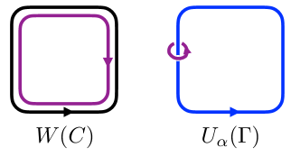
Figure 1: Left: In a confining theory coupled to heavy matter, the expectation value of a large Wilson loop $W(C)$ (black curve) is dominated by contributions that include a large screening ‘matter’ Wilson loop (purple curve) arising from integrating out a charged matter field. Right: The expectation value of $U_{\alpha}(\Gamma)$ (blue curve) is dominated by the contributions of small Wilson loops (purple curve) arising from integrating out the charged matter field.

We start by considering the one-point function of the Gukov-Witten operator in Eq. (5a). The fact that large dynamical Wilson loops $W(C^{\prime})$ come with a suppression factor $e^{-\mu P(C^{\prime})}$ implies that for large $\Gamma$ the sum in Eq. (5a) is dominated by small loops $C^{\prime}\sim 0$. Summing over Wilson loop insertions on small curves $C^{\prime}$ that link $\Gamma$ (illustrated on the right-hand side of Fig. 1) generates perimeter-law behavior for the Gukov-Witten operators

$$\langle U_{\alpha}(\Gamma)\rangle\sim e^{-\mu_{\alpha}P(\Gamma)}\,,$$ (6)

where $\mu_{\alpha}$ is a non-universal mass scale that depends on $\alpha$ as well as e.g. the mass of the charged particle. But we can set $\mu_{\alpha}$ to zero by a counter-term localized on $\Gamma$, producing operators which are topological for large $\Gamma$ so long as $m^{2}\gtrsim g^{4}$. This is consistent with a naive analysis based on the effective field theory Eq. (4).

We now consider Eqs. (5b), (5c). Since $\langle W(C)\rangle_{0}$ has confining behavior, there is a competition between the perimeter-suppression $e^{-\mu P(C^{\prime})}$ of dynamical Wilson loops $W(C^{\prime})$ and the more severe (in this case area-law) suppression of the probe Wilson loop $W(C)$ in the pure gauge theory. As a result, for large contours $C$, large dynamical Wilson loops are favored rather than suppressed, and $\langle W(C)\rangle$ is dominated by fluctuations around the ‘screening loop’ $C^{\prime}=\overline{C}$ running opposite to $C$. This is illustrated in the left-hand side of Fig. 1. Such contributions go to zero with the perimeter of $C$ rather than its area. This is simply the standard physics of screening, which is not captured in the local effective field theory of Eq. (4)! The same conclusion holds for the correlator of the Wilson loop and Gukov-Witten operator in Eq. (5c). Again, the dominant contribution involves a screening loop, and as a result the Gukov-Witten operator measures zero charge.

To summarize, the fact that large Wilson loops are screened implies that their charge cannot be detected at long distances. Instead,

$$\frac{\langle U_{\alpha}(\Gamma)W(C)\rangle}{{\langle U_{\alpha}(\Gamma)\rangle\langle W(C)\rangle}}=1$$ (7)

for well-separated curves $\Gamma,C$ which tend to infinity. Effectively, confinement in the limit $m\to\infty$ (meaning that $\langle W(C)\rangle\to 0$ faster than a perimeter law in that limit) implies that when $m$ is finite all Wilson loops flow to the identity line operator at long distances, leaving nothing for the would-be emergent $1$-form symmetry to act on. As a result the correlation functions of $U_{\alpha}(\Gamma)$ are trivial — all charges are screened. Therefore our emergent-symmetry definition ES is not satisfied, and there is no emergent $1$-form symmetry at finite positive $m^{2}$. Finally, if $-m^{2}\gtrsim g^{4}$, screening loops due to $\phi$ proliferate. Then there is no approximation in which we can neglect the matter field, and so there is also no emergent $1$-form symmetry for $-m^{2}\gtrsim g^{4}$. So there is no reason to expect an emergent $1$-form symmetry for any finite $m^{2}$ in this model.

We conclude that confinement is almost entirely incompatible with the emergence of $1$-form symmetries. For example, there is no infrared-emergent $1$-form symmetry in 4d QCD with fundamental quarks of any finite mass $m_{q}$, no matter how large $m_{q}$ is compared to the strong scale.

V Deconfinement and emergence

We now discuss what happens when an exact $1$-form symmetry is spontaneously broken, and then also explicitly broken by the addition of heavy charged matter fields. To this end, we couple 3d $U(1)$ gauge theory to a charge $N$ scalar $\chi$,

$$S=\int_{M_{3}}\left(\frac{1}{2g^{2}}(da)^{2}+|d\chi-iNa\chi|^{2}+\ldots\right)\,,$$ (8)

and assume $\chi$ is the only electrically-charged field. This theory has an exact $\mathbb{Z}_{N}$ 1-form symmetry generated by Gukov-Witten operators $U_{k}(\Gamma)$, defined to have holonomies $e^{\frac{2\pi ik}{N}}$ on infinitesimal contours linking $\Gamma$. We condense $\chi$, Higgsing the gauge group to $\mathbb{Z}_{N}$. In this phase large Wilson loops have a perimeter-law scaling, and the $1$-form symmetry is spontaneously broken.

We now put in a unit-charge scalar $\phi$ with mass $m$ to explicitly break the $1$-form symmetry. When $m^{2}\gtrsim g^{4}$ the $1$-form symmetry emerges in the long-distance limit with $m$ held fixed. To see this we examine the behavior of the correlation functions in Eq. (5) resulting from formally summing over $\phi$ configurations, with $\langle\cdot\rangle_{0}$ now interpreted as correlation functions of the theory without $\phi$. The analysis of $\langle U_{\alpha}(\Gamma)\rangle$ goes through as before, but the perimeter-law scaling of $\langle W(C)\rangle_{0}$ now implies that small matter loops (as opposed to screening loops with $C^{\prime}\sim\overline{C}$) dominate $\langle U_{\alpha}(\Gamma)W(C)\cdots\rangle$ when $C$ is very large, and

$$\frac{\langle U_{k}(\Gamma)W(C)\rangle}{\langle U_{k}(\Gamma)\rangle\langle W(C)\rangle}=e^{\frac{2\pi ik}{N}\textrm{Link}(\Gamma,C)}$$ (9)

for very large and well-separated loops $C,\Gamma$. Therefore we have a set of operators $U_{\alpha}(\Gamma)$ which have non-trivial topological correlation functions in the long-distance limit, our definition ES is satisfied, and there is an infrared emergent $\mathbb{Z}_{N}$ $1$-form symmetry so long as $\chi$ is condensed and $\phi$ is not.

This analysis resonates with recent discussions of emergent $1$-form symmetries in Refs. Iqbal and McGreevy (2022); Cordova et al. (2022b); Pace and Wen (2022, 2023); Armas and Jain (2023) which assumed (explicitly or implicitly) that they were working in the spontaneously-broken situation discussed in this section. In fact, there is a standard way to understand the above result without invoking the modern language of higher-form symmetries. The charge-$N$ abelian Higgs model flows to a $\mathbb{Z}_{N}$ gauge theory at long distances, described in the continuum by a BF action $S_{\rm BF}=\frac{iN}{2\pi}\int_{M_{3}}b\wedge da$ where $b$ is a (emergent) $U(1)$ $1$-form gauge field, see e.g. Ref. Hansson et al. (2004). This is a topological field theory with $2^{N}$ ground states on a large spatial torus, and it has long been known (see Wen (1991); Vestergren et al. (2005); Hastings and Wen (2005)) that these ground states remain degenerate (and the long-distance BF description remains valid) after the addition of unit-charge matter so long as it does not ‘condense.’ From the more modern perspective, BF theory can be thought of as an effective field theory for a spontaneously-broken $\mathbb{Z}_{N}$ $1$-form symmetry Gaiotto et al. (2015).

VI ’t Hooft anomaly and charged operators

We now explore the interplay between ’t Hooft anomalies and emergent $1$-form symmetries. We again start with $U(1)$ gauge theory in 3d, $S=\int_{M_{3}}\frac{1}{2g^{2}}(da)^{2}$, but this time we do not allow dynamical magnetic monopole-instantons in the UV completion. This gives rise to a 0-form ‘magnetic’ symmetry $U(1)^{(0)}_{m}$ associated with the conserved current $j_{m}^{(1)}=\frac{1}{2\pi}\star da$. This symmetry is generated by topological surface operators $V_{\beta}(\Sigma)$ which act on point-like charge $k$ monopole operators $e^{ik\sigma}$ where $\sigma$ is the $2\pi$-periodic scalar field dual to $a$. As before, the $U(1)^{(1)}_{e}$ electric symmetry is generated by topological line operators $U_{\alpha}(\Gamma)$ which act on charge $q$ Wilson lines $W_{q}(C)$.

The $U(1)^{(0)}_{m}$ and $U(1)^{(1)}_{e}$ symmetries have a mixed ’t Hooft anomaly, see e.g. Gaiotto et al. (2015). This can be detected by turning on $1$-form and $2$-form $U(1)$ background gauge fields $A_{m}$ and $B_{e}$, with $0$-form and $1$-form background gauge transformations $A_{m}\to A_{m}+d\Lambda_{m},B_{e}\to B_{e}+d\Lambda_{e}$, $a\to a+\Lambda_{e}$, so that

$$S[A,B]=\int_{M_{3}}\bigg{[} \frac{1}{2g^{2}}(da-B_{e})^{2}+\frac{i}{2\pi}A_{m}\wedge da$$ (10)

$$-\frac{i}{2\pi}b_{\rm CT}A_{m}\wedge B_{e}+\cdots\bigg{]}$$

where $\cdots$ stands for other background-field counter-terms in addition to the $A_{m}\wedge B_{e}$ term. While it may seem from Eq. (10) one can preserve background gauge invariance for $U(1)^{(0)}_{m}$ by setting $b_{\rm CT}=0$ (or do the same for $U(1)^{(1)}_{e}$ by setting $b_{\rm CT}=1$), the situation is more subtle and is detailed in Appendix A. In any case there is no choice of counterterms which can enforce background gauge invariance for both $A_{m}$ and $B_{e}$ simultaneously, indicating an ’t Hooft anomaly.

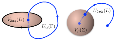
Figure 2: The ’t Hooft anomaly of 3d pure $U(1)$ gauge theory with a $U(1)^{(0)}_{m}\times U(1)^{(1)}_{e}$ symmetry implies that certain unusual correlation functions of the symmetry generators are non-trivial. These correlation functions involve operator intersections (denoted by squares in the figure) and are sensitive to the choice of counter-terms. But it is not possible to fully trivialize the expectation value of the combination of operators given in Eq. (12), which is illustrated in this figure.

The ’t Hooft anomaly implies the following correlation functions:

$$\frac{\langle V_{2\pi q}(D)\,U_{\beta}(\Gamma)\rangle}{\langle V_{2\pi q}(D)\rangle\langle U_{\beta}(\Gamma)\rangle} =e^{iq\beta\,(1-b_{\rm CT})\,\textrm{Link}(\partial D,\Gamma)}\,,$$ (11a)

$$\frac{\langle V_{\alpha}(\Sigma)\,U_{2\pi k}(L)\rangle}{\langle V_{\alpha}(\Sigma)\rangle\langle U_{2\pi k}(L)\rangle} =e^{ik\alpha\,b_{\rm CT}\textrm{Link}(\Sigma,\partial L)}\,,$$ (11b)

where $q,k\in\mathbb{Z}$, and $D$ and $\Sigma$ are (respectively) open and closed surfaces, while $L$ and $\Gamma$ are open and closed lines, which are sketched in Fig. 2. We note that an open surface operator can be modified by attaching an arbitrary line operator to its boundary, with similar remarks holding for open line operators. Our choice in Eq. (11) is such that together, the bulk and boundary of the operators $V_{2\pi q}(D),U_{2\pi k}(L)$ are topological.

Absent the anomaly, $V_{2\pi q}(D)$ would be a trivial surface operator which contributes only contact terms to correlation functions which can all be trivialized by a choice of local counter-terms. But if we take $b_{\rm CT}=0$, Eq. (11a) tells us that the boundary of $V_{2\pi q}(D)$ acts like a charge $q$ topological Wilson line. By comparison, the genuine Wilson lines $W_{q}(C)$, which are not attached to surfaces, are not topological in this model — they are (logarithmically) confined! Similar remarks hold for Eq. (11b), which says that the end-points of $U_{2\pi k}(L)$ behave like a pair of charge $\pm k$ monopole operators (when $b_{\rm CT}=1)$, with only a topological dependence on $L$. In summary, Eq. (11) tells us that in a given scheme the ’t Hooft anomaly adds $V_{2\pi q}(D)$ or $U_{2\pi k}(L)$ to the list of distinct operators charged under $U(1)^{(0)}_{m}$ and $U(1)^{(1)}_{e}$, which would otherwise have only included $W_{q}(C)$ and $e^{ik\sigma}$. The scheme-independent statement is that at least one of the correlators in Eq. (11) is nontrivial. Equivalently, the following correlator is nontrivial in any scheme:

$$\frac{\langle V_{2\pi q}(D)U_{\beta}(\Gamma)\,V_{\alpha}(\Sigma)U_{2\pi k}(L)\rangle}{\langle V_{2\pi q}(D)\rangle\langle U_{\beta}(\Gamma)\rangle\langle V_{\alpha}(\Sigma)\rangle\langle U_{2\pi k}(L)\rangle}\\ =e^{ik\alpha\,b_{\rm CT}\textrm{Link}(\Sigma,\partial L)}\,e^{iq\beta\,(1-b_{\rm CT})\,\textrm{Link}(\partial D,\Gamma)}\not=1.$$ (12)

The quick way to see why Eq. (11) is true is to consider the effects of singular background gauge transformations. An insertion of $V_{2\pi q}(D)$ is equivalent to turning on the background $A_{m}=2\pi q\delta^{(1)}(D)$, which can be removed by a singular gauge transformation $\Lambda_{A}$ which winds by $-2\pi q$ around $\partial D$. Similarly, an insertion of $U_{\beta}(\Gamma)$ with $\Gamma$ contractible is equivalent to taking $B_{e}=\beta\delta^{(2)}(\Gamma)$, which can be removed by the background gauge transformation by $\Lambda_{B}=-\beta\delta^{(1)}(S)$, where $\partial S=\Gamma$. Doing these transformations in $S[A,B]$, we obtain

$$\delta S[A,B] =\frac{i2\pi q\beta(1-b_{\rm CT})}{2\pi}\int_{M_{3}}\delta^{(1)}(D)\wedge\delta^{(2)}(\Gamma)$$

$$=iq\beta(1-b_{\rm CT})\,\textrm{Link}(\partial D,\Gamma)\,,$$ (13)

reproducing Eq. (11a). A very similar computation gives Eq. (11b). We also derive this result in Appendix A using the language of coordinate patches, cochains, and transition functions for readers who are nervous about manipulations of singular gauge transformations. This analysis shows the precise sense in which the ’t Hooft anomaly remains non-trivial even in locally-flat background fields, which is not obvious from its naive form in Eq. (10).

There is a well-known argument that an ’t Hooft anomaly implies that the ground state cannot be trivially gapped. If it were trivially gapped, one could simultaneously gauge both $U(1)^{(0)}_{m}$ and $U(1)^{(1)}_{e}$ in the (empty) long-distance EFT, which would be inconsistent with the ’t Hooft anomaly. The same constraint on the ground state structure follows from Eq. (12). If the ground state on $M_{3}=\mathbb{R}^{3}$ were trivially gapped, then all correlation functions must either go to unity or zero in the long-distance limit. But Eq. (12) is non-trivial for any contractible $\Gamma$ and $\Sigma$, no matter how large, so the ground state on $\mathbb{R}^{3}$ cannot be trivially gapped.

VII ’t Hooft anomaly and emergence

Now we reintroduce our charge-$1$ scalar $\phi$ with mass $m$,

$$S=\int_{M_{3}}\left(\frac{1}{2g^{2}}(da)^{2}+|d\phi-ia\phi|^{2}+m^{2}|\phi|^{2}+\ldots\right)\,,$$ (14)

so that $U(1)^{(1)}_{e}$ is explicitly broken for any finite $m^{2}$. However, in contrast to the analysis after Eq. (3), we continue to assume that there are no dynamical monopole-instantons, so that $U(1)^{(0)}_{m}$ is preserved. The explicit breaking of $U(1)^{(1)}_{e}$ means that the ’t Hooft anomaly seems to be gone, as it no longer makes sense to consider (background) gauging both symmetries. However, is there a range of microscopic parameters for which this QFT has an emergent $1$-form symmetry in the long-distance limit?

This question was considered from the particle-vortex dual perspective Peskin (1978); Dasgupta and Halperin (1981); Karch and Tong (2016) in Ref. Delacrétaz et al. (2020). The authors of Ref. Delacrétaz et al. (2020) argued that the ’t Hooft anomaly of the Nambu-Goldstone effective field theory for a $2+1$d superfluid, which is dual to our $S_{\rm eff}$ from Eq. (4), implies the existence of a robust gapless mode. Here we are posing the question with regard to our definition ES, which requires us to analyze the correlation functions of would-be topological operators.

When $m^{2}$ is sufficiently positive, the discussion following Eq. (5) implies that we can construct approximately-topological operators $U_{\beta}(\Gamma)$ and $U_{2\pi k}(L)$, with $\Gamma$ (resp. $L$) a closed (resp. open) line. However, $\langle W_{q}(C)\rangle\to 0$ faster than a perimeter law when $m^{2}\to\infty$, so $W_{q}(C)$ flows to the trivial operator for large $C$ for any finite $m$. So one may worry that the would-be $1$-form symmetry generators $U_{\beta}(\Gamma)$ have nothing to act on in the long-distance limit.

However, the situation is more interesting. Since $U(1)^{(0)}_{m}$ is not explicitly broken, $V_{2\pi q}(D)$ and $V_{\beta}(\Sigma)$ are topological surface operators. We can now consider Eq. (10) with $B_{e}$ replaced by a $2$-form background field $B$, which can no longer be interpreted as a background gauge field, since $U(1)^{(1)}_{e}$ is explicitly broken. Nevertheless, setting $B=\beta\delta^{(2)}(\Gamma)$ has the effect of inserting a non-topological Gukov-Witten operator $U_{\beta}(\Gamma)$. For large $\Gamma$, however, $U_{\beta}(\Gamma)$ is a approximately topological. If $b_{\rm CT}\neq 1$, $V_{2\pi q}(D)$ has non-trivial approximately-topological correlation functions with $U_{\beta}(\Gamma)$ when $\Gamma$ is large. Crucially, the fact that $V_{2\pi q}(D)$ is exactly topological for any $m^{2}$ means that it is not screened by charged matter loops. If $b_{\rm CT}=1$, the approximately topological operator $U_{2\pi k}(L)$ has non-trivial correlation functions with the exactly topological operator $V_{\beta}(\Sigma)$. Therefore Eq. (11) remains non-trivial in the long-distance limit for sufficiently positive fixed $m^{2}$. Of course if $m^{2}$ is sufficiently negative, matter Wilson loops proliferate, and $U_{\beta}(\Gamma),U_{\beta}(L)$ become non-topological even when $\Gamma$ and $L$ are large.

We thus see that our definition ES is satisfied when $m^{2}$ is sufficiently positive, so that the theory described by Eq. (14) has a $U(1)^{(1)}_{e}$ emergent $1$-form symmetry, despite the fact that the $U(1)^{(1)}_{e}$ symmetry is not spontaneously broken in the limit $m\to\infty$, where test charges are (logarithmically) confined.

VIII Consequences

One interesting consequence of the emergent $U(1)^{(1)}_{e}$ symmetry of 3d massive scalar QED with a $U(1)^{(0)}_{m}$ magnetic symmetry involves its ground state structure. While naively the explicit breaking of the $U(1)^{(1)}_{e}$ kills the mixed ’t Hooft anomaly, the anomaly manages to maintain its grip on the ground state structure thanks to Eq. (11) and the discussion in the preceding section. The non-triviality of Eq. (11) at long distances means that when $m$ is finite (but sufficiently positive) the ground state must remain non-trivial. This is in accordance with Ref. Delacrétaz et al. (2020) which argues that the gapless mode in this regime is a direct consequence of an emergent ’t Hooft anomaly. On the other hand if $m^{2}$ is sufficiently negative, Eq. (11) trivializes. As a result, the ground state can be (and is) trivially gapped, as can be verified by a standard semiclassical calculation, see Fig. 3 for an illustration.

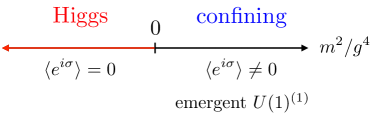
Figure 3: A sketch of the minimal phase diagram of 3d scalar QED, which has Higgs and confining phases which are separated by at least one phase boundary where the realization of the $U(1)_{m}^{(0)}$ symmetry changes and the expectation values of monopole operators $e^{i\sigma}$ are non-analytic. The confining phase is characterized by an emergent $U(1)^{(1)}_{e}$ symmetry.

If we had preserved the $U(1)^{(1)}_{e}$ symmetry but explicitly broken $U(1)^{(0)}_{m}$ by adding unit-charge monopole operators to the action, we would have landed on Eq. (3), a QFT with area-law-like ‘confinement’ (in the same loose sense that QCD with finite mass quarks is confining) and a trivially gapped ground state. This is another illustration of the robustness Wen (1991); Vestergren et al. (2005); Hastings and Wen (2005); Iqbal and McGreevy (2022); Cordova et al. (2022b); Pace and Wen (2022, 2023); Armas and Jain (2023); Verresen et al. (2022); Thorngren et al. (2023) of $1$-form symmetries compared to $0$-form symmetries. Even when $1$-form symmetries are explicitly broken, they can enforce interesting constraints on the low-energy physics, in contrast to $0$-form symmetries.

Another interesting byproduct of the discussion above has to do with Higgs-confinement continuity, namely the common lore that the Higgs and confining regimes of gauge theories with fundamental-representation Higgs fields should be smoothly connected. Higgs-confinement continuity was proven in some lattice models in Refs. Fradkin and Shenker (1979); Banks and Rabinovici (1979), where a key assumption was the absence of any global symmetries under which the Higgs field is charged. The heuristic argument is that in such a situation the Higgs and confining regimes are smoothly connected because there are no order parameters that could distinguish them. The model we have discussed above in Eq. (14) provides an immediate and non-trivial counter-example to the popular interpretation of the results of  Fradkin and Shenker (1979); Banks and Rabinovici (1979) as implying Higgs-confinement continuity even outside the context of the specific models analyzed in those references.

The model in Eq. (14) has a unit-charge Higgs field $\phi$ and a $U(1)^{(0)}_{m}$ global symmetry under which the Higgs field is neutral. The Higgs and confining phases are separated by at least one phase transition where the realization of $U(1)^{(0)}_{m}$ changes, and our results imply that the ‘confining’ phase can be defined as the phase with an emergent $1$-form symmetry, which is separated by at least one phase boundary from the ‘deconfined’ Higgs phase. What makes this counter-example non-trivial is that the Higgs field $\phi$ is not charged under any global symmetry, yet its ‘condensation’ controls the emergent mixed anomaly and subsequent breaking of $U(1)^{(0)}_{m}$. Other possible non-trivial counter-examples to Higgs-confinement continuity in some systems with global symmetries were recently discussed in e.g. Refs. Cherman et al. (2018, 2020).

IX Conclusions

We have put forth necessary conditions for the emergence of 1-form symmetries at long distances. The key requirement is that the long-distance correlation functions of operators be topological and non-trivial. By this criterion, a 1-form symmetry which is not spontaneously broken nor involved in ’t Hooft anomalies cannot emerge at long distances when broken explicitly by finite-mass charged matter. Our definition agrees with the usual lore that the implications of spontaneously-broken higher-form symmetries are robust against explicit breaking. Moreover, the implications of a higher-form symmetry can remain robust against explicit breaking even when the symmetry is not spontaneously broken when the symmetry is involved in an ’t Hooft anomaly.

While for simplicity we focused on 1-form symmetries in 3d, our definition can in principle be applied to higher-form symmetries in any dimension. It would be particularly interesting to analyze a wider class of ’t Hooft anomalies that arise in situations where the higher-form symmetries are not spontaneously broken. For instance, 4d $SU(N)$ $\mathcal{N}=1$ super-YM theory has a $\mathbb{Z}_{N}$ $1$-form symmetry and a $\mathbb{Z}_{N}$ $0$-form symmetry with a mixed ’t Hooft anomaly Gaiotto et al. (2015); Komargodski et al. (2017). If we add a massive fundamental-representation fermion, do we expect an emergent 1-form symmetry at long distances? It is not obvious how to apply arguments similar to those of Sec. VI and Sec. VIII in this paper, because the mixed ’t Hooft anomaly of 4d $\mathcal{N}=1$ SYM is activated at the point-like intersections of Gukov-Witten surface operators, which is not a long-distance correlation function.

It may also be worthwhile to explore the connection of our emergence criterion with the phenomenon of symmetry fractionalization, see e.g. Refs. Jackiw and Rebbi (1976); Senthil and Fisher (2000); Barkeshli et al. (2019); Chen et al. (2015); Nicolas Tarantino (2016); Chen (2017); Brennan et al. (2022); Delmastro et al. (2022), where the charged particles breaking the 1-form symmetry transform in projective representations of a 0-form global symmetry.

Finally, throughout this paper, we focused on the interplay of the large-mass limit, in which the symmetry-breaking matter field contributions are clearly suppressed, and the large-distance limit, where it is less obvious that symmetry breaking effects are suppressed. We should mention that $SU(N)$ QCD has another limit where matter field contributions are clearly suppressed, namely the large $N$ limit where the ’t Hooft coupling, number of flavors $N_{f}$ and mass parameters are fixed as $N\to\infty$. Does a $1$-form symmetry emerge in the large $N$ limit? We recently studied this question together with M. Neuzil in Ref. Cherman et al. (2022). It is well-known that screening of large Wilson loops is $1/N$ suppressed so long as the large $N$ limit is taken before the large-loop limit, so the specific failure mechanism for the emergence of a $1$-form symmetry discussed in the present paper does not apply. However, a $1$-form symmetry fails to emerge anyway, because the $U_{\alpha}(\Gamma)$ operators do not become topological when $N\to\infty$. Their expectation values take the form of Eq. (6) with $\mu_{\alpha}\sim N$, so that $\langle U_{\alpha}(\Gamma)\rangle=0$ at large $N$. It remains an interesting open question whether there is some notion of an ‘emergent symmetry’ which would explain the Wilson loop selection rules of large $N$ QCD.

Appendix A $U(1)^{(0)}\times U(1)^{(1)}$ ’t Hooft anomaly

We give a more precise characterization of the anomaly described in the main text. This allows us to identify operators with non-trivial correlation functions which would not be obvious in a naive continuum approach.

We follow the formalism of Ref. Alvarez (1985), see also Córdova et al. (2020), where we describe gauge fields in terms of patches, transition functions, and cocycle conditions. We choose an open cover $\{U_{I}\}$ of the spacetime manifold. Then we pick an associated partition of the manifold into three-dimensional closed regions $\{\sigma_{I}\}$ with $\sigma_{I}\subset U_{I}$, such that $\sigma_{IJ}=\sigma_{I}\cap\sigma_{J}\subset U_{I}\cap U_{J}$ are 2-dimensional and contained in double overlaps, $\sigma_{IJK}=\sigma_{I}\cap\sigma_{J}\cap\sigma_{K}\subset U_{I}\cap U_{J}\cap U_{K}$ are one-dimensional and contained in triple overlaps, and $\sigma_{IJKL}=\sigma_{I}\cap\sigma_{J}\cap\sigma_{K}\cap\sigma_{L}\subset U_{I}\cap U_{J}\cap U_{K}\cap U_{L}$ are points contained in quadruple overlaps.

The dynamical $U(1)$ gauge field is described by a collection of fields $(a^{(1)}_{I},a^{(0)}_{IJ},a^{(-1)}_{IJK})$. The starting point is an $\mathbb{R}$-valued 1-form gauge field on each patch $a_{I}^{(1)}$. In the language of Ref. Alvarez (1985) this is a 1-form-valued 0-cochain. We use a shorthand notation $\delta$ to take differentials of fields on various overlaps: for instance $(\delta a^{(1)})_{IJ}=a^{(1)}_{J}-a^{(1)}_{I}$. On double overlaps have $(\delta a^{(1)})_{IJ}=da^{(0)}_{IJ}$ where $a^{(0)}_{IJ}\in\mathbb{R}$ is a real-valued, 0-form transition function. Since $a^{(0)}$ has two ‘patch’ indices it is a 1-cochain (with values in 0-forms). It satisfies $(\delta a^{(0)})_{IJK}=a^{(0)}_{JK}-a^{(0)}_{IK}+a^{(0)}_{IJ}=2\pi a^{(-1)}_{IJK}$ with $a^{(-1)}_{IJK}\in\mathbb{Z}$ is a constant integer defined on triple-overlaps (an integer 2-cochain). The $\delta$ operation (which is the coboundary operator) squares to 0 ($\delta^{2}=0$ and commutes with $d$, so that e.g. under an ordinary gauge transformation $(\delta a^{(1)})_{IJ}\to(\delta a^{(1)})_{IJ}+(\delta d\lambda^{(0)})_{IJ}=(\delta a^{(1)})_{IJ}+d(\delta\lambda^{(0)})_{IJ}$. To summarize, the set of relations is

$$(\delta a^{(1)})_{IJ} =da^{(0)}_{IJ},$$ (15a)

$$(\delta a^{(0)})_{IJK} =2\pi\,a^{(-1)}_{IJK},$$ (15b)

$$(\delta a^{(-1)})_{IJKL} =0\,,$$ (15c)

​​​where in the last equation we are looking at quadruple overlaps, and the ‘cocycle condition’ $\delta a^{(-1)}=0$ means there are no magnetic monopoles. The full gauge redundancy is

$$a^{(1)}_{I} \to a^{(1)}_{I}+d\lambda^{(0)}_{I},$$ (16a)

$$a^{(0)}_{IJ} \to a^{(0)}_{IJ}+(\delta\lambda^{(0)})_{IJ}+2\pi\,m^{(-1)}_{IJ},$$ (16b)

$$a^{(-1)}_{IJK} \to a^{(-1)}_{IJK}+(\delta m^{(-1)})_{IJK}\,,$$ (16c)

where the function $\lambda_{I}^{(0)}$ and constants $m_{IJ}^{(-1)}\in\mathbb{Z}$ represent small and large gauge transformations, respectively.

We take the same set of data for the background 1-form $U(1)$ gauge field, $(A_{I}^{(1)},A_{IJ}^{(0)},A^{(-1)}_{IJK})$, where $A^{(1)}$ is a 1-form, $A^{(0)}$ is a 0-form, $A^{(-1)}$ is a constant integer, and $\Lambda^{(0)}_{I}$ and $M^{(-1)}_{IJ}$ will denote the small and large background gauge transformations. In this formalism, a symmetry operator supported on a surface is described by $A_{I}^{(1)}=0$ everywhere and $A^{(0)}_{IJ}$ constant on a set of double-overlaps, so that the corresponding set of $\sigma_{IJ}$’s constitute the surfaces on which the defect is supported. The surface may have a boundary as long as $\delta A^{(0)}$ a multiple of $2\pi$, with $A^{(-1)}_{IJK}$ activated on the boundary. The well-known statement that a generic $U(1)$ background gauge field cannot be expressed in terms of a network of symmetry defects is reflected in the fact that it is possible to activate a non-zero 1-form $A_{I}^{(1)}$ on each patch.

Up to signs, the precise version of $\frac{i}{2\pi}\int A\wedge da$ is

$$``\frac{i}{2\pi}\int A\wedge da"=\frac{i}{2\pi}\sum_{I}\int_{\sigma_{I}}A_{I}^{(1)}\wedge da_{I}^{(1)}\\ +\frac{i}{2\pi}\sum_{I<J}\int_{\sigma_{IJ}}A^{(0)}_{IJ}\wedge da^{(1)}_{J}-\frac{i}{2\pi}\sum_{I<J<K}A^{(-1)}_{IJK}\int_{\sigma_{IJK}}a_{K}^{(1)}\\ -i\sum_{I<J<K<L}\left.A^{(-1)}_{IJK}\,a^{(0)}_{KL}\right|_{\sigma_{IJKL}}\,.$$ (17)

It is invariant under gauge transformations of all fields and is well-defined. What happens if we turn on $A^{(-1)}_{IJK}=q$ on some triple overlap? First, we see that this inserts a Wilson line, and the cocycle condition on $A^{(-1)}$ implies that this line must be closed. Second, the relations between $A^{{(-1)}}_{IJK}$ and neighboring $A^{{(0)}}_{IJ}$ implies that we must also turn on $A^{(0)}_{IJ}=2\pi q$ on some neighboring double overlap, which inserts a field-strength surface operator involving $da^{(1)}$ on that overlap. This gives a rigorous definition of the operator $V_{2\pi q}(D)$ in Eq. (11) the main text.

The 2-form gauge field is described by $(B_{I}^{(2)},B^{(1)}_{IJ},B^{(0)}_{IJK},B^{(-1)}_{IJKL})$. Here $B^{(2)}$ is a real 2-form on each patch, $B^{(1)}$ is a real 1-form on double overlaps, $B^{(0)}$ is a real 0-form on triple overlaps, and $B^{(-1)}$ is a constant integer on quadruple overlaps. They are related via

$$(\delta B^{(2)})_{IJ} =dB^{(1)}_{IJ},$$ (18a)

$$(\delta B^{(1)})_{IJK} =dB^{(0)}_{IJK},$$ (18b)

$$(\delta B^{(0)})_{IJKL} =2\pi\,B^{(-1)}_{IJKL}\,.$$ (18c)

Under gauge transformations we have

$$B^{(2)}_{I} \to B^{(2)}_{I}+d\Pi^{(1)}_{I},$$ (19a)

$$B^{(1)}_{IJ} \to B^{(1)}_{IJ}+(\delta\Pi^{(1)})_{IJ}+d\Pi^{(0)}_{IJ},$$ (19b)

$$B^{(0)}_{IJK} \to B^{(0)}_{IJK}+(\delta\Pi^{0})_{IJK}+2\pi L^{(-1)}_{IJK},$$ (19c)

$$B^{(-1)}_{IJKL} \to B^{(-1)}_{IJKL}+(\delta L^{(-1)})_{IJKL}\,,$$ (19d)

where $\Pi^{(1)}_{I}$ is a real 1-form, $\Pi^{0}_{IJ}$ is a real 0-form, $L^{(-1)}_{IJK}$ is a constant integer. Again, a generic 2-form $U(1)$ gauge field cannot be associated with a network of symmetry defects, but if $B^{(2)}=0,B^{(1)}=0$ we can think of $B^{(0)}$ activated on a set of triple-overlaps as inserting a codimension-2 symmetry defect on lines (corresponding to a set of $\sigma_{IJK}$’s).

The dynamical gauge field $a^{(1)}$ shifts under background 1-form gauge transformations. Accordingly, in the presence of the background field for the 1-form symmetry the relations Eq. (15) are modified to

$$(\delta a^{(1)})_{IJ} =da^{(0)}_{IJ}+B^{(1)}_{IJ},$$ (20a)

$$(\delta a^{(0)})_{IJK} =2\pi a^{(-1)}_{IJK}-B^{(0)}_{IJK},$$ (20b)

$$(\delta a^{(-1)})_{IJKL} =B^{(-1)}_{IJKL}\,.$$ (20c)

These relations are invariant under the background gauge transformations

$$a^{(1)}_{I} \to a^{(1)}_{I}+\Pi^{(1)}_{I},$$ (21a)

$$a^{(0)}_{IJ} \to a^{(0)}_{IJ}-\Pi^{(0)}_{IJ},$$ (21b)

$$a^{(-1)}_{IJK} \to a^{(-1)}_{IJK}+L^{(-1)}_{IJK}\,.$$ (21c)

The anomalous shift of Eq. (17) under 1-form background gauge transformations is then

$$\frac{i}{2\pi}\sum_{I}\int_{\sigma_{I}}A^{(1)}_{I}\wedge d\Pi^{(1)}_{I}+\frac{i}{2\pi}\sum_{I<J}\int_{\sigma_{IJ}}A^{(0)}_{IJ}\wedge d\Pi^{(1)}_{J}\\ -\frac{i}{2\pi}\sum_{I<J<K}A^{(-1)}_{IJK}\int_{\sigma_{IJK}}\Pi^{(1)}_{K}\\ +i\sum_{I<J<K<L}\left.A^{(-1)}_{IJK}\,\Pi^{(0)}_{KL}\right|_{\sigma_{IJKL}}\,,$$ (22)

As we mentioned above, if we insert $V_{2\pi q}(D)$ by taking $A^{(0)}_{IJ}=2\pi q$ on a set of double-overlaps tiling $D$, we must also have $A^{(-1)}_{IJK}=\pm q$ on the set of triple overlaps containing the boundary of $D$. We now insert $U_{\beta}(\Gamma)$ by setting $B^{(0)}_{IJK}$ equal to a constant $\beta$ on the triple overlaps tiling the closed loop $\Gamma$, which we assume pierces $D$. Removing this curve with an appropriate 1-form gauge transformation with $\Pi^{(0)}=\beta$, we pick up a phase $e^{i\beta q}$ from the last term above. This reproduces Eq. (11a) in the main text, except that we have not yet discussed the counter-term dependence.

We also have anomalous shifts of Eq. (17) involving 0-form gauge transformations of $A$ coming from the modified cocycle condition Eq. (21c),

$$-\frac{i}{2\pi}\sum_{I<J}\int_{\sigma_{IJ}}\Lambda^{(0)}_{I}\wedge dB^{(1)}_{IJ}-i\sum_{I<J<K}M^{(-1)}_{IJ}\int_{\sigma_{IJK}}B^{(1)}_{JK}\\ +i\sum_{I<J<K<L}\left.M^{(-1)}_{IJ}\,B^{(0)}_{JKL}\right|_{\sigma_{IJKL}}\,.$$ (23)

We can now contemplate adding various counter-terms involving $B$. In particular if we add

$$``\frac{-i}{2\pi}\int A\wedge B"=-\frac{i}{2\pi}\sum_{I}\int_{\sigma_{I}}A_{I}^{(1)}\wedge B_{I}^{(2)}$$ (24)

$$-\frac{i}{2\pi}\sum_{I<J}\int_{\sigma_{IJ}}A^{(0)}_{IJ}\wedge B^{(2)}_{J}-\frac{i}{2\pi}\sum_{I<J<K<L}\left.A^{(0)}_{IJ}\,B^{(0)}_{JKL}\right|_{\sigma_{IJKL}}\,,$$

then we can cancel all the terms in Eq. (23) and the first two terms in Eq. (22). This is equivalent to setting $b_{\text{CT}}=1$ in Eq. Eq. (10). We then have

$$``\frac{i}{2\pi}\int A\wedge(da-B)"=\frac{i}{2\pi}\sum_{I}\int_{\sigma_{I}}A^{(1)}_{I}\wedge(da^{(1)}-B^{(2)})_{I}$$

$$+\frac{i}{2\pi}\sum_{I<J}\int_{\sigma_{IJ}}A^{(0)}_{IJ}\wedge(da^{(1)}-B^{(2)})_{J}$$

$$-\frac{i}{2\pi}\sum_{I<J<K}A^{(-1)}_{IJK}\int_{\sigma_{IJK}}a^{(1)}_{K}$$

$$-i\sum_{I<J<K<L}\left.A^{(-1)}_{IJK}\,a^{(0)}_{KL}\right|_{\sigma_{IJKL}}$$

$$-\frac{i}{2\pi}\sum_{I<J<K<L}\left.A^{(0)}_{IJ}\,B^{(0)}_{JKL}\right|_{\sigma_{IJKL}}\,,$$ (25)

The anomalous shift of Eq. (25) is

$$S_{\text{anomaly},b_{\text{CT}}=1}$$ (26)

$$=-i\sum_{I<J}M^{(-1)}_{IJ}\int_{\sigma_{IJ}}B^{(2)}_{J}-\frac{i}{2\pi}\sum_{I<J<K}A^{(-1)}_{IJK}\int_{\sigma_{IJK}}\Pi^{(1)}_{K}$$

$$+i\sum_{I<J<K<L}\left.A^{(-1)}_{IJK}\,\Pi^{(0)}_{KL}\right|_{\sigma_{IJKL}}$$

$$-\frac{i}{2\pi}\sum_{I<J<K<L}\left.A^{(0)}_{IJ}(\delta\Pi^{(0)}+2\pi L^{(-1)})_{JKL}\right|_{\sigma_{IJKL}}$$

$$-i\sum_{I<J<K<L}\left.M^{(-1)}_{IJ}\,(\delta\Pi^{(0)})_{JKL}\right|_{\sigma_{IJKL}}$$

$$-\frac{i}{2\pi}\sum_{I<J<K<L}\left.(\delta\Lambda^{(0)})_{IJ}\,B^{(0)}_{JKL}\right|_{\sigma_{IJKL}}$$

Now if we consider the same configuration from before with $A^{(0)}_{IJ}=2\pi q,A^{(-1)}_{IJK}=q$, the two terms above in the second and third line cancel and $\langle V_{2\pi q}(D)U_{\beta}(\Gamma)\rangle$ has no non-trivial phases.

However, we can consider a configuration where $B^{(0)}_{IJK}=2\pi k$ on a set of triple-overlaps containing an open line $L$, with $B^{(-1)}_{IJKL}=\pm k$ at the quadruple overlaps containing the endpoints of $L$. This represents the insertion of an open generator of the $2\pi$ 1-form transformation $U_{2\pi k}(L)$ (which would be trivial absent an anomaly). If we also insert a 0-form generator $V_{\alpha}(\Sigma)$ on a closed surface $\Sigma$ enclosing the endpoint, with $A^{(0)}_{IJ}=\alpha$ for some constant $\alpha$ on an appropriate set of double-overlaps containing $\Sigma$, then the gauge transformation $A^{(0)}_{IJ}\to A^{(0)}_{IJ}+(\delta\Lambda^{(0)})_{IJ}$ used to unlink the surface $\Sigma$ from the the endpoint of the 1-form generator $U_{2\pi k}(L)$ will yield the phase $e^{i\alpha k}$ from the last term in Eq. (26). This reproduces Eq. (11b) for the behavior of $\langle V_{\alpha}(\Sigma)U_{2\pi k}(L)\rangle$.

References

- Gaiotto et al. (2015) Davide Gaiotto, Anton Kapustin, Nathan Seiberg, and Brian Willett, “Generalized Global Symmetries,” JHEP 02, 172 (2015), arXiv:1412.5148 [hep-th] .
- McGreevy (2022) John McGreevy, “Generalized Symmetries in Condensed Matter,” (2022), arXiv:2204.03045 [cond-mat.str-el] .
- Cordova et al. (2022a) Clay Cordova, Thomas T. Dumitrescu, Kenneth Intriligator, and Shu-Heng Shao, “Snowmass White Paper: Generalized Symmetries in Quantum Field Theory and Beyond,” in 2022 Snowmass Summer Study (2022) arXiv:2205.09545 [hep-th] .
- Iqbal and McGreevy (2022) Nabil Iqbal and John McGreevy, “Mean string field theory: Landau-Ginzburg theory for 1-form symmetries,” SciPost Phys. 13, 114 (2022), arXiv:2106.12610 [hep-th] .
- Delacrétaz et al. (2020) Luca V. Delacrétaz, Diego M. Hofman, and Grégoire Mathys, “Superfluids as Higher-form Anomalies,” SciPost Phys. 8, 047 (2020), arXiv:1908.06977 [hep-th] .
- Cordova et al. (2022b) Clay Cordova, Kantaro Ohmori, and Tom Rudelius, “Generalized Symmetry Breaking Scales and Weak Gravity Conjectures,” (2022b), arXiv:2202.05866 [hep-th] .
- Pace and Wen (2022) Salvatore D. Pace and Xiao-Gang Wen, “Emergent Higher-Symmetry Protected Topological Orders in the Confined Phase of Gauge Theory,” (2022), arXiv:2207.03544 [cond-mat.str-el] .
- Pace and Wen (2023) Salvatore D. Pace and Xiao-Gang Wen, “Exact emergent higher symmetries in bosonic lattice models,” (2023), arXiv:2301.05261 [cond-mat.str-el] .
- Armas and Jain (2023) Jay Armas and Akash Jain, “Approximate higher-form symmetries, topological defects, and dynamical phase transitions,” (2023), arXiv:2301.09628 [hep-th] .
- Cherman et al. (2022) Aleksey Cherman, Theodore Jacobson, and Maria Neuzil, “1-form symmetry versus large N QCD,” (2022), arXiv:2209.00027 [hep-th] .
- Hsin and Turzillo (2020) Po-Shen Hsin and Alex Turzillo, “Symmetry-enriched quantum spin liquids in (3 + 1),” JHEP 09, 022 (2020), arXiv:1904.11550 [cond-mat.str-el] .
- Rudelius and Shao (2020) Tom Rudelius and Shu-Heng Shao, “Topological Operators and Completeness of Spectrum in Discrete Gauge Theories,” JHEP 12, 172 (2020), arXiv:2006.10052 [hep-th] .
- Kapustin and Seiberg (2014) Anton Kapustin and Nathan Seiberg, “Coupling a QFT to a TQFT and Duality,” JHEP 04, 001 (2014), arXiv:1401.0740 [hep-th] .
- Polyakov (1977) Alexander M. Polyakov, “Quark confinement and topology of gauge groups,” Nucl. Phys. B120, 429–458 (1977).
- Montvay and Munster (1997) I. Montvay and G. Munster, Quantum fields on a lattice, Cambridge Monographs on Mathematical Physics (Cambridge University Press, 1997).
- Feynman (1950) R. P. Feynman, “Mathematical formulation of the quantum theory of electromagnetic interaction,” Phys. Rev. 80, 440–457 (1950).
- Feynman (1951) Richard P. Feynman, “An Operator calculus having applications in quantum electrodynamics,” Phys. Rev. 84, 108–128 (1951).
- Bern and Kosower (1991) Zvi Bern and David A. Kosower, “Efficient calculation of one loop QCD amplitudes,” Phys. Rev. Lett. 66, 1669–1672 (1991).
- Bern and Kosower (1992) Zvi Bern and David A. Kosower, “The Computation of loop amplitudes in gauge theories,” Nucl. Phys. B 379, 451–561 (1992).
- Strassler (1992) Matthew J. Strassler, “Field theory without Feynman diagrams: One loop effective actions,” Nucl. Phys. B 385, 145–184 (1992), arXiv:hep-ph/9205205 .
- Hansson et al. (2004) T. H. Hansson, Vadim Oganesyan, and S. L. Sondhi, “Superconductors are topologically ordered,” Annals Phys. 313, 497–538 (2004).
- Wen (1991) Xiao-Gang Wen, “Topological orders and Chern-Simons theory in strongly correlated quantum liquid,” Int. J. Mod. Phys. B 5, 1641–1648 (1991).
- Vestergren et al. (2005) A Vestergren, J Lidmar, and T. H Hansson, “Topological order in the (2+1)d compact lattice superconductor,” Europhysics Letters (EPL) 69, 256–262 (2005).
- Hastings and Wen (2005) M. B. Hastings and Xiao-Gang Wen, “Quasiadiabatic continuation of quantum states: The stability of topological ground-state degeneracy and emergent gauge invariance,” Physical Review B 72 (2005), 10.1103/physrevb.72.045141.
- Peskin (1978) Michael E. Peskin, “Mandelstam ’t Hooft Duality in Abelian Lattice Models,” Annals Phys. 113, 122 (1978).
- Dasgupta and Halperin (1981) C. Dasgupta and B. I. Halperin, “Phase Transition in a Lattice Model of Superconductivity,” Phys. Rev. Lett. 47, 1556–1560 (1981).
- Karch and Tong (2016) Andreas Karch and David Tong, “Particle-Vortex Duality from 3d Bosonization,” Phys. Rev. X 6, 031043 (2016), arXiv:1606.01893 [hep-th] .
- Verresen et al. (2022) Ruben Verresen, Umberto Borla, Ashvin Vishwanath, Sergej Moroz, and Ryan Thorngren, “Higgs Condensates are Symmetry-Protected Topological Phases: I. Discrete Symmetries,” (2022), arXiv:2211.01376 [cond-mat.str-el] .
- Thorngren et al. (2023) Ryan Thorngren, Tibor Rakovszky, Ruben Verresen, and Ashvin Vishwanath, “Higgs Condensates are Symmetry-Protected Topological Phases: II. Gauge Theory and Superconductors,” (2023), arXiv:2303.08136 [cond-mat.str-el] .
- Fradkin and Shenker (1979) Eduardo H. Fradkin and Stephen H. Shenker, “Phase Diagrams of Lattice Gauge Theories with Higgs Fields,” Phys. Rev. D 19, 3682–3697 (1979).
- Banks and Rabinovici (1979) Tom Banks and Eliezer Rabinovici, “Finite Temperature Behavior of the Lattice Abelian Higgs Model,” Nucl. Phys. B 160, 349–379 (1979).
- Cherman et al. (2018) Aleksey Cherman, Srimoyee Sen, and Laurence G. Yaffe, “Anyonic particle-vortex statistics and the nature of dense quark matter,” (2018), arXiv:1808.04827 [hep-th] .
- Cherman et al. (2020) Aleksey Cherman, Theodore Jacobson, Srimoyee Sen, and Laurence G. Yaffe, “Higgs-confinement phase transitions with fundamental representation matter,” Phys. Rev. D 102, 105021 (2020), arXiv:2007.08539 [hep-th] .
- Komargodski et al. (2017) Zohar Komargodski, Tin Sulejmanpasic, and Mithat Ünsal, “Walls, anomalies, and (de)confinement in quantum anti-ferromagnets,” (2017), arXiv:1706.05731 [cond-mat.str-el] .
- Jackiw and Rebbi (1976) R. Jackiw and C. Rebbi, “Solitons with Fermion Number 1/2,” Phys. Rev. D13, 3398–3409 (1976).
- Senthil and Fisher (2000) T. Senthil and Matthew P. A. Fisher, “ gauge theory of electron fractionalization in strongly correlated systems,” Phys. Rev. B 62, 7850–7881 (2000).
- Barkeshli et al. (2019) Maissam Barkeshli, Parsa Bonderson, Meng Cheng, and Zhenghan Wang, “Symmetry fractionalization, defects, and gauging of topological phases,” Phys. Rev. B 100, 115147 (2019).
- Chen et al. (2015) Xie Chen, F. J. Burnell, Ashvin Vishwanath, and Lukasz Fidkowski, “Anomalous symmetry fractionalization and surface topological order,” Phys. Rev. X 5, 041013 (2015).
- Nicolas Tarantino (2016) Lukasz Fidkowski Nicolas Tarantino, Netanel H Lindner, “Symmetry fractionalization and twist defects,” New Journal of Physics 18 (2016), 10.1088/1367-2630/18/3/035006.
- Chen (2017) Xie Chen, “Symmetry fractionalization in two dimensional topological phases,” Reviews in Physics 2, 3–18 (2017).
- Brennan et al. (2022) T. Daniel Brennan, Clay Cordova, and Thomas T. Dumitrescu, “Line Defect Quantum Numbers & Anomalies,” (2022), arXiv:2206.15401 [hep-th] .
- Delmastro et al. (2022) Diego Delmastro, Jaume Gomis, Po-Shen Hsin, and Zohar Komargodski, “Anomalies and Symmetry Fractionalization,” (2022), arXiv:2206.15118 [hep-th] .
- Alvarez (1985) Orlando Alvarez, “Topological Quantization and Cohomology,” Commun. Math. Phys. 100, 279 (1985).
- Córdova et al. (2020) Clay Córdova, Daniel S. Freed, Ho Tat Lam, and Nathan Seiberg, “Anomalies in the Space of Coupling Constants and Their Dynamical Applications I,” SciPost Phys. 8, 001 (2020), arXiv:1905.09315 [hep-th] .