Zhang, Liu, and Zhao

Data-driven PADR for SP with Covariate Information

Data-driven Piecewise Affine Decision Rules for Stochastic Programming with Covariate Information

Yiyang Zhang Department of Industrial Engineering, Tsinghua University, Beijing 100084, China, zyy21@mails.tsinghua.edu.cn Junyi Liu Department of Industrial Engineering, Tsinghua University, Beijing 100084, China, junyiliu@tsinghua.edu.cn Xiaobo Zhao Department of Industrial Engineering, Tsinghua University, Beijing 100084, China, xbzhao@tsinghua.edu.cn

Focusing on stochastic programming (SP) with covariate information, this paper proposes an empirical risk minimization (ERM) method embedded within a nonconvex piecewise affine decision rule (PADR), which aims to learn the direct mapping from features to optimal decisions. We establish the nonasymptotic consistency result of our PADR-based ERM model for unconstrained problems and asymptotic consistency result for constrained ones. To solve the nonconvex and nondifferentiable ERM problem, we develop an enhanced stochastic majorization-minimization algorithm and establish the asymptotic convergence to (composite strong) directional stationarity along with complexity analysis. We show that the proposed PADR-based ERM method applies to a broad class of nonconvex SP problems with theoretical consistency guarantees and computational tractability. Our numerical study demonstrates the superior performance of PADR-based ERM methods compared to state-of-the-art approaches under various settings, with significantly lower costs, less computation time, and robustness to feature dimensions and nonlinearity of the underlying dependency.

stochastic programming, covariate information, decision rule, piecewise affine function, nonconvex and nondifferentiable optimization programming: nondifferentiable; nonlinear; stochastic

1 Introduction

Pioneered by George Dantzig in the mid-1950s, stochastic programming (SP) provides a class of optimization models for decision-making under uncertainty by treating the uncertainty as a random variable whose probability distribution is usually unknown in practice. With the growing real-world applications and availability of large datasets, the field of SP has flourished with many theoretical and algorithmic advances (Birge and Louveaux 2011, Shapiro et al. 2021), in which the empirical probability distribution based on historical scenarios plays a central role in approximating the true distribution. However, the empirical distribution may provide poor estimation when the random variable is related to covariate information (also referred to as contextual information or features) which can be observed before the decision is made. An unconstrained SP with the covariate information $X=x\in\mathbb{R}^{p}$ is formulated as follows,

$$\inf_{z\in\mathbb{R}^{d}}\quad\mathbb{E}_{Y}\left[\varphi({z};{Y})\mid X=x\right],$$ (1)

where $z\in\mathbb{R}^{d}$ is a decision vector, $\varphi:\mathbb{R}^{d}\times\mathcal{Y}\to\mathbb{R}$ is a cost function, and $Y$ is a random variable supported by $\mathcal{Y}$ whose distribution is related to a feature vector $X$ supported by $\mathcal{X}\subseteq\mathbb{R}^{p}$. A simple instance is an inventory planning problem, in which $z$ represents order decisions for $d$ products, $\varphi$ represents the inventory cost, $Y$ represents uncertain demands, and $X$ represents covariate information such as seasonality, promotion, and weather. With historical scenarios of $(X,Y)$, a classical sample average approximation (SAA) model disregards the dependency of $Y$ on $X$ and thus may lead to inconsistent decisions; such deficiency is also observed in numerical results of Ban and Rudin (2018) and Bertsimas and Koduri (2021). Motivated by the latent dependency of the optimal solution to (1) on the feature vector, this paper aims to construct a data-driven decision rule that directly maps features to optimal decisions so as to approximately solve the SP problem (1) for any possible observation of the feature.

1.1 Problem Setting

Solving problem (1) for any realization of $X$ can be generalized as seeking an optimal decision rule (DR) to the following problem

$$\inf_{f\in\mathcal{F}}\quad R(f)\coloneqq\mathbb{E}_{X,Y}\left[\varphi({f(X)};{Y})\right],$$ (2)

where $\mathcal{F}$ contains all measurable functions mapping from the feature space $\mathcal{X}$ to the decision space $\mathbb{R}^{d}$. By the interchangeability principle (Shapiro et al. 2021, Theorem 7.80), if a mapping $f^{*}\in\mathcal{F}$ is optimal to problem (2), then the decision $f^{*}(x)$ is optimal to (1) for almost every $x\in\mathcal{X}$. In general, problem (2) is intractable due to the infinite-dimensional function space and the unknown joint distribution of $X$ and $Y$. A common approximation method is to construct an empirical risk minimization (ERM) problem based on a dataset $S\coloneqq\{(x^{s},y^{s})\}_{s=1}^{n}$ with the decision rule $f$ restricted to a parametric DR class $\mathcal{H}$ (also known as hypothesis class):

$$\inf_{f\in\mathcal{H}}\quad\widehat{R}_{S}(f)\coloneqq\frac{1}{n}\sum_{s=1}^{n}\varphi({f(x^{s})};{y^{s}}).$$ (3)

In this paper, we adopt the above DR-based ERM framework, recognizing that the efficacy of such a framework is influenced by the trade-off between approximation accuracy of $\mathcal{H}$ to the optimal DR $f^{*}$ and computational complexity of solving (3). For example, problem (3) with a convex cost function can be solved efficiently with $\mathcal{H}$ being the class of linear decision rules (LDR) (Beutel and Minner 2012, Ban and Rudin 2018), while the LDR has difficulty describing the potential nonlinear relation between decisions and features. On the other side, a DR class consisting of neural networks could have a strong approximation capability (Qi et al. 2022); nevertheless, the resulting nonconvex problem (3) with a multi-layer composite structure is difficult to solve with theoretical optimality guarantees, and the model may face overfitting issues when the dataset is not large enough.

Therefore, this paper aims to address a critical question: what could be an amenable hypothesis class for the DR-based ERM framework so as to maintain both high reliability and computational efficiency for solving SP with covariate information? To this end, we employ in the ERM problem (3) a piecewise affine decision rule (PADR) that is broader than LDR but simpler than general nonlinear DRs. According to Scholtes (2012), any continuous piecewise affine (PA) function $f:\mathcal{X}\rightarrow\mathbb{R}$ can be expressed as the difference of max-affine functions:

$$f(x;\theta)=\max_{k\in[K]}\left\{(\alpha^{k})^{\top}x+a^{k}\right\}-\max_{k\in[K]}\left\{(\beta^{k})^{\top}x+b^{k}\right\},$$ (4)

where $\theta\coloneqq\left(\alpha^{k},a^{k},\beta^{k},b^{k}\right)_{k=1}^{K}\in\mathbb{R}^{2K(p+1)}$ and $[K]\coloneqq\{1,\dots,K\}$. Throughout the theoretical analysis in this paper, we assume that the numbers of pieces in the two max-affine components of (4) are equal to simplify the exposition, which could be easily extended to the case with different numbers of pieces. With $\mathcal{H}$ being the class of continuous PA functions with each max-affine component having $K$ pieces and parameters $\{\theta_{\iota}\}_{\iota\in[d]}$ satisfying $\left\lVert\theta_{\iota}\right\rVert_{\infty}\leq\mu$ for $\iota\in[d]$, the ERM problem (3) is formulated as the following parameter estimation problem

$$\min_{\left\lVert\theta_{\iota}\right\rVert_{\infty}\leq\mu,\forall\iota\in[d]}\quad\frac{1}{n}\sum_{s=1}^{n}\varphi\left(\Big{(}\max_{k\in[K]}\left\{(\alpha^{k}_{\iota})^{\top}x^{s}+a^{k}_{\iota}\right\}-\max_{k\in[K]}\left\{(\beta^{k}_{\iota})^{\top}x^{s}+b^{k}_{\iota}\right\}\Big{)}_{\iota=1}^{d};y^{s}\right).$$ (5)

In response to the aforementioned question, we intend to tackle two critical issues of the PADR-based ERM model in this paper: the consistency issue of the PADR-based ERM problem (5) and the computational issue for solving this large-scale, nonconvex, and nondifferentiable composite optimization problem. We address the first issue by quantifying the excess risk bound of our model, a standard procedure for model selection (Bartlett et al. 2002) in machine learning, and the second issue by developing a sampling-based algorithm with convergence guarantees, through which we demonstrate the ability of our proposed PADR-based ERM approach to effectively solve a broad class of SP problems with covariate information.

1.2 Literature Review

We present a literature review of data-driven methods for SP with covariate information and algorithmic advances in solving nonconvex optimization problems.

1.2.1 SP with Covariate Information.

There are two main schemes of data-driven approaches in the literature of SP dealing with the latent dependency on covariate information: the sequential and integrated schemes. In the sequential scheme, also referred to as the predict-then-optimize (PO) scheme (Deng and Sen 2022, Kannan et al. 2022), one first predicts uncertain parameters and then solves the optimization problem composite with the prediction model. Several works such as Kao et al. (2009), Donti et al. (2017), and Elmachtoub and Grigas (2021) propose modifications of the loss function by accounting for the cost error of the downstream optimization problem. Since those modified loss functions involve optimal solutions to the decision-making problems that are parameterized by suspicious prediction models, such frameworks usually lead to bi-level nonconvex optimization problems and thus encounter substantial computational challenges in dealing with general constrained nonlinear programs.

Approaches in the integrated scheme yield decisions via one-step data-driven optimization. Bertsimas and Kallus (2019) and Kallus and Mao (2022) approximate the conditional expected cost in (1) by a reweighted empirical cost. However, as claimed by Bertsimas and Koduri (2021), this framework is highly affected by the data with features close to the current observation and thus suffers from the curse of dimensionality. The DR-based ERM framework presented in (3) is another one-step approach in the integrated scheme. Due to its functional approximation in nature, this approach is relieved from the aforementioned issue.

Besides the classical LDR, several generalized LDRs are proposed for standard SP problems which lift random vectors into a higher-dimensional probability space to describe nonlinear relations (Chen et al. 2007, Bampou and Kuhn 2011, Georghiou et al. 2015). However, they tend to have unsatisfactory performance without cautious prior designs especially when the random vector is high-dimensional; moreover, except for the posterior estimation provided in Kuhn et al. (2011), their approximation accuracy lacks theoretical guarantees. The PADR with the parametric formula (4) employed in Bertsimas and Georghiou (2015) and this paper requires no prior designs of breakpoints as in Georghiou et al. (2015); instead, the breakpoints are implicitly determined by parameters in (4). Unlike the mixed-integer formulation in Bertsimas and Georghiou (2015) for multi-stage adaptive optimization problems, we treat the PADR-based ERM problem (5) as a special class of nonconvex and nondifferentiable optimization problems and exploit algorithmic advances to accommodate the large sample size and high-dimensional feature space.

Several works on DR-based ERM methods are most relevant to this paper. Ban and Rudin (2018) employ LDR for the Newsvendor problem with nonasymptotic optimality guarantees under the assumption of the linear demand model. Notz and Pibernik (2021) and Bertsimas and Koduri (2021) study decision rules in reproducing kernel Hilbert spaces (RKHS), which we refer to as RKHS-DR, and provide asymptotic optimality guarantees for convex SP problems. Compared to the above references, our PADR-based ERM model is suitable for a much broader class of SP problems that can be nonconvex, and by following the statistical learning theory (Vapnik 1999, Mohri et al. 2018), we establish the nonasymptotic consistency result of our model without any parametric assumptions on the optimal decision rule or the latent dependency of the random variable $Y$ on the feature $X$.

1.2.2 Difference-of-convex (DC) and Composite DC Programming.

Due to the finite-sum composite structure of the objective in (5) with potentially large sample size $n$ and feature dimension $p$, it is prohibitively challenging to obtain a global minimizer to such a nonconvex and nondifferentiable optimization problem. Thus, our goal is to compute a promising candidate for a local minimizer via a sampling-based algorithm.

When the cost function $\varphi(\cdot;y)$ is piecewise affine (e.g., the Newsvendor cost), the overall composite objective of (5) is also piecewise affine, which is a special DC function. Deterministic DC algorithms have been extensively studied for solving DC programs over the last several decades (Le Thi and Pham Dinh 2018). When the concave part of the DC decomposition is nondifferentiable, the basic DC algorithm converges to a critical point that satisfies the necessary condition for local optimality. To obtain a d(irectional)-stationary point that is the sharpest first-order stationary point for general nonconvex problems, Pang et al. (2016) study a class of nondifferentiable DC programs whose concave part is the maximum of a finite number of smooth convex functions and propose an enhanced DC algorithm which iteratively solves convex subproblems constructed by linearizing the $\varepsilon$-active piece of the concave part. Though sampling-based algorithms for stochastic DC programs have been recently studied in Nitanda and Suzuki (2017), Xu et al. (2019), and Le Thi et al. (2022) addressing smooth or partially smooth objectives, there still lacks a comprehensive study of the enhanced surrogation technique in stochastic DC algorithms to seek d-stationary solutions to the stochastic DC programs with nondifferentiable concave parts.

With a more general cost function that is not necessarily piecewise affine, the finite-sum composite structure of the objective lies at the cornerstone of algorithmic development for solving the PADR-based ERM problem (5). Cui et al. (2018) study the ERM problem with a convex composite DC structure and develop a majorization-minimization (MM) algorithm with an enhanced surrogation technique similar to Pang et al. (2016); however, such a deterministic algorithm requires iteratively solving finite-sum convex subproblems over all the data, raising concerns about its computational efficiency for solving large-scale ERM problems. The composite DC problem (5) can be regarded as a special class of compound SP studied in Liu et al. (2022) with finite support and solved by the stochastic majorization-minimization (SMM) algorithm proposed by the authors. Nonetheless, without the enhanced surrogation technique, SMM can only asymptotically compute a compound critical point when the inner concave function is nondifferentiable. Finally, we refer readers to Cui and Pang (2021) for a comprehensive study of modern nonconvex and nondifferentiable optimization, especially Chapters 6 and 7 for the study of stationary concepts and surrogation-based algorithms for nonconvex composite optimization problems.

1.3 Contributions

We summarize our major contributions as follows.

1. We propose a PADR-based ERM method for a general class of SP problems with covariate information, where both cost and constraint functions can be nonconvex. We quantify the approximation accuracy of the PA function class and establish the nonasymptotic consistency result of our framework for unconstrained problems and asymptotic consistency result for deterministic-constrained problems without any parametric assumptions on the optimal decision rule or the latent dependency.

2. For learning PADR from the ERM problem, we develop an enhanced SMM algorithm with asymptotic convergence to composite strong d-stationarity, which is a sharper stationary concept than d-stationarity specialized to the composite DC programs with PA inner functions. We further provide nonasymptotic convergence of the algorithm to d-stationarity, which to the best of our knowledge is the first complexity result for stochastic nonsmooth composite DC programs. The enhanced SMM algorithm is also extended with exact penalization for solving the PADR-based ERM problem with constraints.

3. We test our method through numerical experiments on the Newsvendor problem and its variations with comparisons to the PO methods and other prominent DR-based methods, including the (generalized) LDR and RKHS-DR. The results demonstrate the superior performance of our method with significantly lower costs and less computation time in most instances, particularly those with high-dimensional redundant features or highly nonlinear models.

The rest of this paper is organized as follows. In Section 2, we provide the theoretical consistency result of the PADR-based ERM model. We then develop the enhanced SMM algorithm for learning PADR with surrogation construction of composite PA objectives in Section 3 and present the convergence analysis in Section 4. In Section 5, we extend our framework to deterministic-constrained SP problems. In Section 6, we report numerical results. We end with conclusions in Section 7.

2 Theoretical Guarantees for PADR-based ERM

In this section, we provide theoretical guarantees of the PADR-based ERM model by first quantifying the approximation error of the PA function class to Lipschitz continuous functions and then presenting the nonasymptotic consistency result of the PADR-based ERM model via the excess risk bound. At the end of this section, we compare our theoretical results with prominent ERM models employing the LDR and RKHS-DR.

2.1 Approximation Accuracy of Piecewise Affine Function Class

PA functions are known to asymptotically approximate Lipschitz continuous functions. Balazs et al. (2015) and Siahkamari et al. (2020) quantify the approximation errors of the PA function class to convex and DC functions, respectively. We provide the approximation bound of the PA function class to Lipschitz continuous functions, which to the best of our knowledge is the first quantification result for such a general case. Specifically, with $L>0$ and $M>0$, let

$$\mathcal{F}_{L,M}\coloneqq\left\{f:\mathcal{X}\rightarrow\mathbb{R}^{d}\mid\left\lVert f\right\rVert_{\infty}\leq M,\,\text{$f$ is $L$-Lipschitz continuous}\right\},$$

where $\left\lVert f\right\rVert_{\infty}\coloneqq\sup_{x\in\mathcal{X}}\max_{\iota\in[d]}|f_{\iota}(x)|$. We define the PADR class ${\mathcal{H}}_{\mu}^{K}$ as

$$\mathcal{H}^{K}_{\mu}\coloneqq\left\{\left(f_{\iota}(\,\cdot\,;\theta_{\iota}):\mathcal{X}\rightarrow\mathbb{R}\right)_{\iota=1}^{d}\ \middle|\ \begin{aligned} &f_{\iota}(x;\theta_{\iota})=\max_{k\in[K]}\left\{(\alpha^{k}_{\iota})^{\top}x+a^{k}_{\iota}\right\}-\max_{k\in[K]}\left\{(\beta^{k}_{\iota})^{\top}x+b^{k}_{\iota}\right\},\\ &\theta_{\iota}\coloneqq\left(\alpha_{\iota}^{k},a_{\iota}^{k},\beta_{\iota}^{k},b_{\iota}^{k}\right)_{k=1}^{K}\in\mathbb{R}^{2K(p+1)},\left\lVert\theta_{\iota}\right\rVert_{\infty}\leq\mu,\,\forall\,\iota\in[d]\end{aligned}\ \right\}.$$ (6)

When $K=1$, $\mathcal{H}^{1}_{\mu}$ reduces to the LDR class. We provide the approximation bound of the PA function class to Lipschitz continuous functions below with the proof given in Appendix 8.1.

Proposition 2.1 (Approximation Bound of ${\mathcal{H}}_{\mu}^{K}$)

Suppose that $\mathcal{X}\subseteq\mathbb{R}^{p}$ is a compact set with $\max_{x\in\mathcal{X}}\left\lVert x\right\rVert_{\infty}=\bar{X}$. Then given $L_{0}>0$ and $M_{0}>0$, for any $f_{0}\in\mathcal{F}_{L_{0},M_{0}}$ and ${\mathcal{H}}_{\mu}^{K}$ defined in (6) with $K\in\mathbb{N}$ and $\mu\geq\max\left\{\frac{1}{2}L_{0}K^{1/p},\frac{1}{4}pL_{0}\bar{X}K^{1/p}+\frac{1}{2}M_{0}\right\}$, we have

$$\min_{f\in\mathcal{H}_{\mu}^{K}}\left\lVert f-f_{0}\right\rVert_{\infty}\leq 2(p^{1/2}+3)p^{1/2}L_{0}\bar{X}K^{-1/p}.$$

The bound $\mathcal{O}(K^{-1/p})$ provided in Proposition 2.1 is weaker than $\mathcal{O}(K^{-2/p})$ given by Balazs et al. (2015) and Siahkamari et al. (2020) in approximating convex and DC functions. Regardless, our bound is applicable to general PA-based statistical learning problems in which the underlying true model may not be convex or DC; more importantly, it renders the succeeding nonasymptotic consistency result of the PADR-based ERM model without any parametric or convex assumptions on the optimal decision rule or latent dependency.

2.2 Nonasymptotic Consistency of PADR-based ERM

We impose the following assumptions for the consistency analysis:

1. Samples in $S=\{(x^{s},y^{s})\}_{s=1}^{n}$ of $(X,Y)$ are independently and identically distributed.

2. For some $\bar{X}>0$, the support set $\mathcal{X}\subseteq\mathbb{R}^{p}$ of $X$ is a compact set with $\max_{x\in\mathcal{X}}\left\lVert x\right\rVert_{\infty}=\bar{X}$.

3. For some $L_{\varphi}>0$, $C_{\varphi}>0$, $z_{0}\in\mathbb{R}^{d}$, and any $y\in\mathcal{Y}$, the cost function $\varphi({\cdot};{y})$ is Lipschitz continuous on $\mathbb{R}^{d}$ with modulus $L_{\varphi}$ and satisfies $\left\lvert\varphi(z_{0};y)\right\rvert\leq C_{\varphi}$.

4. There exists a Lipschitz continuous function $f^{*}:\mathcal{X}\rightarrow\mathbb{R}^{d}$ that is optimal to problem (2).

The boundedness of $\mathcal{X}$ in Assumption (A2) is common in practical applications. Under Assumption (A2), the optimal DR $f^{*}$ in Assumption (A4) is bounded on $\mathcal{X}$, and thus $f^{*}\in\mathcal{F}_{L_{z},M_{z}}$ for some $L_{z}>0$ and $M_{z}>0$.

With the optimal solution to (5) denoted by $f^{*}_{S,{\mathcal{H}}_{\mu}^{K}}$, the consistency of the PADR-based ERM model is evaluated by the excess risk $R(f^{*}_{S,{\mathcal{H}}_{\mu}^{K}})-\underset{f\in\mathcal{F}}{\inf}\,R(f)$, which is the gap between the expected cost of the optimal empirical PADR and the minimal cost. With problem (2) restricted to ${\mathcal{H}}_{\mu}^{K}$, we decompose the excess risk into the approximation and estimation errors as follows,

$$R(f^{*}_{S,{\mathcal{H}}_{\mu}^{K}})-\inf_{f\in\mathcal{F}}R(f)=\underbrace{R(f^{*}_{S,{\mathcal{H}}_{\mu}^{K}})-\min_{f\in{\mathcal{H}}_{\mu}^{K}}R(f)}_{\text{estimation error}}+\underbrace{\min_{f\in{\mathcal{H}}_{\mu}^{K}}R(f)-\inf_{f\in\mathcal{F}}R(f)}_{\text{approximation error}}.$$ (7)

The approximation error measures the gap between the expected costs induced by the optimal PADR and the optimal DR, which can be bounded via the approximation bound of ${\mathcal{H}}_{\mu}^{K}$ in Proposition 2.1 under Assumption (A4); the estimation error measures the gap between the expected costs induced by the PADR solutions to the empirical and expected problems respectively, which is bounded via the uniform generalization bound stated below. Note that in this paper the notation $\left\lVert\cdot\right\rVert$ without a subscript refers to the Euclidean norm.

Proposition 2.2 (Uniform Generalization Bound of PADR-based ERM)

Under Assumptions (A1)-(A3), with $M_{\mu}\coloneqq C_{\varphi}+L_{\varphi}\left(2\sqrt{d}\mu(p\bar{X}+1)+\left\lVert z_{0}\right\rVert\right)$, the following holds with probability at least $1-\delta$ over the draw of $S$,

$$\max_{f\in{\mathcal{H}}_{\mu}^{K}}\left\lvert R(f)-\widehat{R}_{S}(f)\right\rvert\leq\frac{8\mu L_{\varphi}\sqrt{2dK(p+1)(p\bar{X}^{2}+1)}}{n}+2M_{\mu}\sqrt{\frac{2dK(p+1)\log n}{n}}+\sqrt{2}M_{\mu}\sqrt{\frac{\log(2/\delta)}{n}}.$$

The proof based on the Rademacher complexity theory is presented in Appendix 8.2. Combining the approximation and estimation error bounds, we obtain the excess risk bound of PADR-based ERM in Theorem 2.3 with the proof in Appendix 8.2.

Theorem 2.3 (Excess Risk Bound of PADR-based ERM)

Under Assumptions (A1)-(A4), with $\mu\geq\max\left\{\frac{1}{2}L_{z}K^{1/p},\frac{1}{4}pL_{z}\bar{X}K^{1/p}+\frac{1}{2}M_{z}\right\}$ and $M_{\mu}\coloneqq C_{\varphi}+L_{\varphi}\left(2\sqrt{d}\mu(p\bar{X}+1)+\left\lVert z_{0}\right\rVert\right)$, the following holds with probability at least $1-\delta$ over the draw of $S$,

$$R(f^{*}_{S,{\mathcal{H}}_{\mu}^{K}})\,\leq\, \inf_{f\in\mathcal{F}}R(f)+2d^{1/2}(p^{1/2}+3)p^{1/2}L_{\varphi}L_{z}\bar{X}K^{-1/p}$$

$$+\frac{16\mu L_{\varphi}\sqrt{2dK(p+1)(p\bar{X}^{2}+1)}}{n}+4M_{\mu}\sqrt{\frac{2dK(p+1)\log n}{n}}+2\sqrt{2}M_{\mu}\sqrt{\frac{\log(2/\delta)}{n}}.$$

With $\mu=\mathcal{O}(K^{1/p})$, the complexity of the excess risk bound with respect to the sample size $n$ and parameter $K$ is

$$R(f^{*}_{S,{\mathcal{H}}_{\mu}^{K}})-\inf_{f\in\mathcal{F}}R(f)=\underbrace{\widetilde{\mathcal{O}}\left(K^{\frac{p+2}{2p}}n^{-\frac{1}{2}}\right)}_{\begin{subarray}{c}\text{estimation}\\ \text{error bound}\end{subarray}}+\underbrace{\mathcal{O}\left(K^{-\frac{1}{p}}\right)}_{\begin{subarray}{c}\text{approximation}\\ \text{error bound}\end{subarray}},$$ (8)

where $\widetilde{\mathcal{O}}(\cdot)$ suppresses logarithmic factors. It can be seen that the sample size $n$ only affects the estimation error, whereas $K$, the number of max-affine pieces for PA functions in ${\mathcal{H}}_{\mu}^{K}$, plays the central role of balancing the two error terms. As $K$ grows, the PA function class becomes larger, so the approximation error decreases due to the stronger approximation ability of ${\mathcal{H}}_{\mu}^{K}$, and the estimation error increases due to the more pronounced overfitting issue. By setting $K=\mathcal{O}(n^{p/(p+4)})$, we derive the optimal excess risk bound $\widetilde{\mathcal{O}}(n^{-{1}/(4+p)})$.

2.3 Consistency Comparison with Existing DR-based Methods

We compare the consistency result of the PADR-based ERM model with two prominent types of DR-based ERM methods in Table 2.3. Both the methods NV-ERM1 and NV-ERM2 from Ban and Rudin (2018) employ LDR, the latter of which additionally applies regularization in the objective. We use $\text{RKHS-DR}_{\text{NP}}$ and $\text{RKHS-DR}_{\text{BK}}$ to represent RKHS-DR methods from Notz and Pibernik (2021) and Bertsimas and Koduri (2021) respectively, so as to distinguish that the former imposes regularization via constraints, while the latter applies regularization in the objective.

Comparison of Error Bounds for Multiple DR-based ERM Models. Problem Type Method Approximation Error Estimation Error Excess Risk Convex NV-ERM1 0 (Linear asm.) $\widetilde{\mathcal{O}}(n^{-\frac{1}{2+p/2}})$ $\widetilde{\mathcal{O}}(n^{-\frac{1}{2+p/2}})$ NV-ERM2 0 (Linear asm.) $\geq\mathcal{O}(n^{-\frac{1}{2+p/4}})$ / $\text{RKHS-DR}_{\text{NP}}$ / $\mathcal{O}(n^{-\frac{1}{2}})$ / $\text{RKHS-DR}_{\text{BK}}$ 0 $\geq\mathcal{O}(n^{-\frac{1}{2}})$ / Nonconvex PADR $\mathcal{O}(K^{-\frac{1}{p}})$ $\widetilde{\mathcal{O}}(K^{\frac{p+2}{2p}}n^{-\frac{1}{2}})$ $\widetilde{\mathcal{O}}(n^{-\frac{1}{4+p}})$ The complexity with “$\geq$” means that the error is only bounded partly. The notation “/” means that the error bound is not provided.

Out of the four benchmarks considered in the literature, only Ban and Rudin (2018) provide an excess risk bound for NV-ERM1, which leverages the special structure of the Newsvendor problem with a linear true demand model. The estimation error bounds for NV-ERM2 and $\text{RKHS-DR}_{\text{BK}}$ are not provided due to the unknown regularization bias. There is no approximation error for $\text{RKHS-DR}_{\text{BK}}$ since an RKHS with a universal kernel is dense in the space of continuous functions, while such an error of $\text{RKHS-DR}_{\text{NP}}$ with a norm-constrained RKHS plausibly exists but is not analyzed in Notz and Pibernik (2021). It should be noted that the theoretical analysis for all benchmarks, except $\text{RKHS-DR}_{\text{NP}}$ , is restricted to convex SP problems.

In comparison, our PADR-based ERM model is nonasymptotically consistent for general SP problems, including nonconvex ones. Moreover, if there exists a convex or DC optimal DR, based on the approximation bounds $\mathcal{O}(K^{-2/p})$ of ${\mathcal{H}}_{\mu}^{K}$ from Balazs et al. (2015) and Siahkamari et al. (2020), our excess risk bound can be improved to $\widetilde{\mathcal{O}}(n^{-1/(3+p/2)})$ with $K=\mathcal{O}(n^{p/(p+6)})$, which is close to the bound of NV-ERM1 (a special case of our model) when $p$ is large. This gap will vanish, that is, the bound can be further refined to $\widetilde{\mathcal{O}}(n^{-1/(2+p/2)})$ for SP with a box-constrained set $[-M,M]^{d}$, by employing a truncated PADR class ${\bar{\mathcal{H}}}_{\mu}^{K}\coloneqq\{\bar{f}\mid\bar{f}=\max\{\min\{f,M\},-M\},\,f\in{\mathcal{H}}_{\mu}^{K}\}$ in (3), under which $M_{\mu}$ in Theorem 2.3 could be independent of $\mu$.

Though obtaining the global optimum $f^{*}_{S,{\mathcal{H}}_{\mu}^{K}}$ of the nonconvex ERM problem (5) is prohibitively challenging, we show in Sections 3 and 4 how to asymptotically compute a stationary solution that could be globally optimal to problem (5) under particular algorithmic settings, upon which our PADR-based ERM framework is asymptotically optimal.

3 Enhanced SMM Algorithm for Learning PADR

In this section, we focus on learning PADR by solving problem (5). Following the majorization-minimization (MM) framework, we develop a stochastic algorithm that iteratively solves convex subproblems constructed with sampling-based enhanced surrogation functions, referred to as an enhanced SMM algorithm. The highlight of our algorithm that distinguishes itself from the deterministic MM-related algorithms in Pang et al. (2016) and Cui et al. (2018) and stochastic ones in Xu et al. (2019), Le Thi et al. (2022), and Liu et al. (2022) is that it combines the enhanced $\varepsilon$-active surrogation technique with sequential sampling so as to converge to d-stationary solutions with a significant improvement of computational efficiency.

We first make some remarks on notations to facilitate algorithmic development and convergence analysis. With a slight abuse of notation, to emphasize the role of PADR as a function of $\theta$, we represent the PA function as $f(\theta;\xi)=g(\theta;\xi)-h(\theta;\xi)$ with $\xi\in S=\{(x^{s},y^{s})\}_{s=1}^{n}$, where $g(\theta;\xi)\coloneqq\max_{i\in[K]}g_{i}(\theta;\xi)$ and $h(\theta;\xi)\coloneqq\max_{i\in[K]}h_{i}(\theta;\xi)$ are maximum of linear functions. With $\widetilde{\xi}_{n}$ representing a random variable uniformly distributed on $S$, the PADR-based ERM problem (5) can be generalized as the following stochastic program with finite support:

$$\min_{\theta\in\Theta}\quad F(\theta)\coloneqq\mathbb{E}\,\left[\varphi(f(\theta;\widetilde{\xi}_{n});\widetilde{\xi}_{n})\right],$$ (9)

where $\Theta\subseteq\mathbb{R}^{q}$ is a compact convex set. In particular, in problem (5) with $\Theta=[-\mu,\mu]^{q}$ and $q=2dK(p+1)$, the outer function $\varphi(\cdot;\xi)$ with $\xi=(x,y)$ depends solely on $y$, and the inner PA function $f(\cdot;\xi)$ depends solely on $x$.

3.1 Construction of Surrogation Functions

Similar to other MM-related algorithms, the cornerstone of the enhanced SMM algorithm is the construction of surrogation functions of $F(\cdot;\xi)\coloneqq\varphi(f(\cdot;\xi);\xi)$. For a directionally differentiable function $\phi:\Theta\to\mathbb{R}$, that is, the directional derivative $\phi^{\prime}(\theta;d)\coloneqq\lim_{\tau\to 0}\frac{\phi(\theta+\tau d)-\phi(\theta)}{\tau}$ exists for any $\theta\in\Theta$ and $d\in\mathbb{R}^{q}$, we are interested in constructing a surrogation function $\widehat{\phi}(\cdot;\theta^{\prime})$ at a reference point $\theta^{\prime}\in\Theta$ that may satisfy the following conditions:

1. Touching condition: $\widehat{\phi}(\theta^{\prime};\theta^{\prime})=\phi(\theta^{\prime})$.

2. Majorizing condition: $\widehat{\phi}({\theta};{\theta^{\prime}})\geq\phi(\theta)$ for any $\theta\in\Theta$.

3. Convexity: $\widehat{\phi}({\cdot};{\theta^{\prime}})$ is convex on $\Theta$.

4. Directional derivative consistency: $\widehat{\phi}(\cdot;\theta^{\prime})$ is directionally differentiable on $\Theta$ and satisfies $\widehat{\phi}(\cdot;\theta^{\prime})^{\prime}(\theta^{\prime};d)=\phi^{\prime}(\theta^{\prime};d)$ for any $d\in\mathbb{R}^{q}$.

5. Quadratic surrogation gap: for some $\kappa>0$, $\phi(\theta)+\displaystyle{\frac{\kappa}{2}}\left\lVert\theta-\theta^{\prime}\right\rVert^{2}\geq\widehat{\phi}(\theta;\theta^{\prime})$ for any $\theta\in\Theta$.

A function satisfying the first two conditions is referred to as an upper surrogation function according to Cui and Pang (2021, Definition 7.1.1). Though the enhanced $\varepsilon$-active surrogation functions to be constructed generally do not satisfy (P1), we still refer to ones solely satisfying (P2) as upper surrogation functions and similarly for lower surrogation functions. Condition (P3) ensures that surrogation-based subproblems in the algorithm can be solved by convex-programming solvers. Condition (P4) connecting the directional derivatives of surrogation and original functions is used to establish stationarity conditions of the limit points produced by surrogation-based algorithms to the original problem. Condition (P5) originating from Liu et al. (2022) is a technical condition for the nonasymptotic convergence analysis of the enhanced SMM algorithm. Note that Condition (P5) implies (P4) provided that $\widehat{\phi}(\cdot;\theta^{\prime})$ is directionally differentiable and satisfies (P2).

We first present upper and lower surrogation functions of the inner PA function $f(\cdot;\xi)$, which provide the basis of surrogation construction of $F(\cdot;\xi)$ and also play an essential role in the randomized index-mapping selection in the enhanced SMM algorithm. For $d=1$ and $\varepsilon\geq 0$, let $\mathcal{I}_{g}^{\varepsilon}(\theta^{\prime})$ denote the set of $\varepsilon$-active index mappings for functions $\{g(\cdot;\xi)\}_{\xi\in S}$ at $\theta^{\prime}\in\Theta$, i.e.,

$$\mathcal{I}_{g}^{\varepsilon}(\theta^{\prime})\coloneqq\Big{\{}I_{1}:S\rightarrow[K]\mid\,g_{I_{1}(\xi)}(\theta^{\prime};\xi)\geq g(\theta^{\prime};\xi)-\varepsilon,\,\forall\,\xi\in S\Big{\}},$$

and the set $\mathcal{I}_{h}^{\varepsilon}(\theta^{\prime})$ is similarly defined for $\{h(\cdot;\xi)\}_{\xi\in S}$. Each mapping $I_{1}\in\mathcal{I}_{g}^{\varepsilon}(\theta^{\prime})$ assigns an $\varepsilon$-active index for each $\xi\in S$, and thus $\{I_{1}(\xi)\}_{\xi\in S}$ constitutes an $\varepsilon$-active index combination of $\{g(\cdot;\xi)\}_{\xi\in S}$ at $\theta^{\prime}$. It is clear to see that $\widehat{f}(\theta;\xi,I_{2})\coloneqq g(\theta;\xi)-h_{I_{2}(\xi)}(\theta;\xi)$ with $I_{2}\in\mathcal{I}_{h}^{\varepsilon}(\theta^{\prime})$ is an upper surrogation function of $f(\cdot;\xi)$ satisfying Conditions (P2) and (P3) with $\varepsilon\geq 0$, and additionally (P1) with $\varepsilon=0$. The concave lower surrogation function $\widecheck{f}(\theta;\xi,I_{1})$ with $I_{1}\in\mathcal{I}_{g}^{\varepsilon}(\theta^{\prime})$ can be similarly defined. When $d>1$, the index mapping sets and surrogates are constructed componentwisely.

Now, we can construct the upper surrogation function of $F(\cdot;\xi)$ at a reference point $\theta^{\prime}$ based on the surrogation of inner PA functions with the index mapping $I\in\mathcal{I}^{\varepsilon}(\theta^{\prime})\coloneqq\mathcal{I}_{g}^{\varepsilon}(\theta^{\prime})\times\mathcal{I}_{h}^{\varepsilon}(\theta^{\prime})$, which we denote by $\widehat{F}(\cdot;\theta^{\prime},\xi,I)$. To facilitate the convergence analysis of the enhanced SMM algorithm, we impose the following assumptions on the family of surrogates $\{\widehat{F}(\cdot;\theta^{\prime},\xi,I)\}_{I\in\mathcal{I}^{\varepsilon}(\theta^{\prime})}$:

1. The family of surrogates $\{\widehat{F}(\cdot;\theta^{\prime},\xi,I)\}_{I\in\mathcal{I}^{\varepsilon}(\theta^{\prime})}$ for any $\xi\in S$ satisfy the following properties:

   1. $\widehat{F}(\cdot;\theta^{\prime},\xi,I)$ satisfies Conditions (P2) and (P3) for every $I\in\mathcal{I}^{\varepsilon}(\theta^{\prime})$ with $\varepsilon\geq 0$;

   2. $\widehat{F}(\cdot;\theta^{\prime},\xi,I)$ satisfies Condition (P1) for every $I\in\mathcal{I}^{0}(\theta^{\prime})$;

   3. $\widehat{F}(\cdot;\cdot,\xi,I)$ is continuous on $\Theta\times\Theta$ given a fixed index mapping $I$;

   4. the minimum surrogate $\widehat{F}^{\varepsilon}_{\min}(\theta;\theta^{\prime},\xi)\coloneqq\min_{I\in\mathcal{I}^{\varepsilon}(\theta^{\prime})}\widehat{F}(\theta;\theta^{\prime},\xi,I)$ satisfies Condition (P4) for any $\varepsilon\geq 0$.

2. The minimum surrogate $\widehat{F}^{\varepsilon}_{\min}(\theta;\theta^{\prime},\xi)$ satisfies Condition (P5) for any $\varepsilon\geq 0$ and $\xi\in S$.

To illustrate the specific construction of surrogation functions satisfying the above assumptions, we consider the following three cases of the outer function $\varphi$:

1. $\varphi(\cdot;\xi)$ is piecewise affine for any $\xi\in S$.

2. $\varphi(\cdot;\xi)$ can be decomposed into monotonic convex functions for any $\xi\in S$.

3. $\varphi(\cdot;\xi)$ is smooth with Lipschitz gradient for any $\xi\in S$.

In Appendix 9, we provide the surrogation construction of $F(\cdot;\xi)$ for these cases with verification of Assumptions (B1) and (B2). The three cases cover a broad class of cost functions. In particular, Case 2 is a multivariate extension of the one considered in Cui et al. (2018), which shows that any univariate convex function can be written as the sum of monotonic convex functions. The surrogation construction for Case 3 is new and suitable for nonconvex smooth cost functions.

3.2 Enhanced SMM Algorithm

We present the enhanced SMM algorithm in Algorithm 1.

Input: initial point $\theta^{0}$, iteration length $T$, parameters $\{\eta,\varepsilon\}$, and increasing sequence $\{N_{\nu}\}_{\nu}$;

1 for $\nu=0$ to $T-1$ do

2       for $s=1,\dots,N_{\nu}$, draw $\xi_{\nu}^{s}$ independently and uniformly from $S$;

3       select $I_{\nu}^{\varepsilon}$ uniformly from $\mathcal{I}^{\varepsilon}(\theta^{\nu})$;

4       compute $\theta^{\nu+\frac{1}{2}}\in\underset{\theta\in\Theta}{\mathop{\arg\min}}\left\{\widehat{F}_{N_{\nu}}(\theta;\theta^{\nu},I_{\nu}^{\varepsilon})+\frac{\eta}{2}\left\lVert\theta-\theta^{\nu}\right\rVert^{2}\right\}$;

5       update the iterate $\theta^{\nu+1}=\begin{cases}\theta^{\nu+\frac{1}{2}},&\text{if}\ \widehat{F}_{N_{\nu}}(\theta^{\nu+\frac{1}{2}};\theta^{\nu},I_{\nu}^{\varepsilon})+\frac{\eta}{2}\lVert\theta^{\nu+\frac{1}{2}}-\theta^{\nu}\rVert^{2}\leq F_{N_{\nu}}(\theta^{\nu}),\\ \theta^{\nu},&\text{otherwise.}\end{cases}$

6 end for

Output: $\widetilde{\theta}^{\,T}$ uniformly sampled from the iterates $\{\theta^{\nu}\}_{\nu=0}^{T-1}$.

Algorithm 1 Enhanced SMM Algorithm

At iteration $\nu$, with samples $\{\xi_{\nu}^{s}\}_{s=1}^{N_{\nu}}$ and an $\varepsilon$-active index mapping $I^{\varepsilon}_{\nu}\in\mathcal{I}^{\varepsilon}(\theta^{\nu})$ randomly selected in Steps 2 and 3, we compute in Step 4 the proximal mapping point $\theta^{\nu+\frac{1}{2}}$ with respect to the upper surrogation function $\widehat{F}_{N_{\nu}}(\cdot;\theta^{\nu},I_{\nu}^{\varepsilon})\coloneqq\frac{1}{N_{\nu}}\sum_{s=1}^{N_{\nu}}\widehat{F}(\cdot;\theta^{\nu},\xi_{\nu}^{s},I^{\varepsilon}_{\nu})$ of the sample average approximation function $F_{N_{\nu}}(\cdot)\coloneqq\frac{1}{N_{\nu}}\sum_{s=1}^{N_{\nu}}F(\cdot;\xi_{\nu}^{s})$. Since the surrogate function value $\widehat{F}_{N_{\nu}}(\theta^{\nu};\theta^{\nu},I_{\nu}^{\varepsilon})$ could be strictly larger than $F_{N_{\nu}}(\theta^{\nu})$, the candidate point $\theta^{\nu+\frac{1}{2}}$ may not lead to a valid update. Hence, it is accepted in Step 5 only when sufficient descent is satisfied. In the special case of $\varepsilon=0$, the touching condition (P1) is satisfied. Thus the proximal mapping point $\theta^{\nu+\frac{1}{2}}$ naturally satisfies the sufficient descent inequality in Step 5, and we directly update $\theta^{\nu+1}=\theta^{\nu+\frac{1}{2}}$.

It is worth noticing that the randomized index-mapping selection in Step 3 is vital for the ERM problem, without which the number of subproblems to be solved at each iteration, identical with the cardinality of $\mathcal{I}^{\varepsilon}(\theta^{\nu})$, would grow exponentially with the sample size. Furthermore, by combining the enhanced $\varepsilon$-active surrogation with incremental sample averaging, the enhanced SMM can achieve satisfactory descent progress in early iterations with relatively small sample sizes, thus improving the computational efficiency; yet such a combination raises the major challenges of convergence analysis to be addressed in the next section.

4 Convergence Analysis of Enhanced SMM

In this section, we first introduce preliminaries on stationarity concepts and then analyze the convergence properties of the enhanced SMM algorithm for solving problem (9). Since much of the convergence analysis is quite technical, we present the main theoretical results with essential discussions while leaving analytical details in Appendix 10.

4.1 Preliminaries on Stationarity

Suppose that the outer function $\varphi$ is Bouligand-differentiable (B-differentiable), i.e., it is locally Lipschitz continuous and directionally differentiable on $\mathbb{R}^{d}$. Then the composite function $F$ is also B-differentiable according to Cui and Pang (2021, Proposition 4.1.2). We say that $\theta^{d}\in\Theta$ is a d-stationary point of problem (9) if $F^{\prime}(\theta^{d};\theta-\theta^{d})\geq 0$ for any $\theta\in\Theta$. For a general nonconvex problem on a convex set, d-stationarity is identified as the sharpest among the first-order stationarity concepts, which gives a necessary condition for local optimality. Specialized to the composite DC program (9), it is equivalent to local optimality if $\varphi$ is in Case 1 or Case 2 (Cui et al. 2018, Proposition 2), and more generally we further define the following strengthened d-stationarity.

Definition 4.1

Given $\varepsilon\geq 0$ and $\rho>0$, we say that $\theta^{d}\in\Theta$ is a composite $(\varepsilon,\rho)$-strongly d-stationary point of problem (9) if $\displaystyle{\{\theta^{d}\}=\mathop{\arg\min}_{\theta\in\Theta}\left\{\min_{I\in\mathcal{I}^{\varepsilon}(\theta^{d})}\widehat{F}(\theta;\theta^{d},I)+\frac{\rho}{2}\left\lVert\theta-\theta^{d}\right\rVert^{2}\right\}}$, where $\widehat{F}(\theta;\theta^{d},I)\coloneqq\mathbb{E}\,[\widehat{F}(\theta;\theta^{d},\widetilde{\xi}_{n},I)\,]$, and $\{\widehat{F}(\cdot;\theta^{d},\xi,I)\}_{I\in\mathcal{I}^{\varepsilon}(\theta^{d})}$ satisfy Assumption (B1) for every $\xi\in S$.

This concept is generalized from the $(\alpha,\eta)$-d-stationarity defined in Lu et al. (2019) for structured DC programs. Due to the requirement of the unique proximal mapping point in the defining condition, our concept is slightly stronger for a reduced composite DC program with the identity outer function $\varphi$. Moreover, it is weaker than the composite $\varepsilon$-strong d-stationarity introduced in Qi et al. (2021) (see also Cui and Pang (2021, Definition 6.1.3)) due to the presence of an additional proximal term in the defining condition that is necessary for the follow-up convergence analysis.

Let $\mathcal{S}^{d}$, $\mathcal{S}^{d}_{\varepsilon,\rho}$, and $\mathcal{S}^{*}$ denote the sets of d-stationary points, composite $(\varepsilon,\rho)$-strongly d-stationary points, and global minimizers of (9), respectively. We show below that the composite strong d-stationarity is stronger than d-stationarity and necessary for global optimality.

Proposition 4.2

Under Assumption (B1) for the surrogate family $\{\widehat{F}(\cdot;\theta^{\prime},\xi,I)\}_{I\in\mathcal{I}^{\varepsilon}(\theta^{\prime})}$ of $F(\cdot;\xi)$ for each $\xi\in S$, it holds for problem (9) that $\mathcal{S}^{*}\subseteq\mathcal{S}^{d}_{\varepsilon,\rho}\subseteq\mathcal{S}^{d}$ for any $\varepsilon\geq 0$ and $\rho>0$. In particular, $\mathcal{S}^{d}_{0,\rho}=\mathcal{S}^{d}$ for any $\rho>0$.

The proof is provided in Appendix 10.1. Furthermore, we can show that $\mathcal{S}^{*}=\mathcal{S}^{d}_{\varepsilon,\rho}$ for sufficiently large $\varepsilon$ and suitable $\rho$ under Assumption (B2) and a regularity condition that d-stationary values of problem (9) are isolated from the optimal value, which naturally hold when $\varphi$ is in Case 1 or Case 2; this is formally stated as Proposition 10.2 in Appendix 10.1.

4.2 Convergence Analysis of Enhanced SMM Algorithm

Now we establish the convergence analysis of Algorithm 1 in terms of (composite strong) d-stationarity for problem (9). Throughout this section, we make several blanket assumptions that the outer function $\varphi$ is B-differentiable, $\Theta$ is a compact convex set, and the surrogate family $\{\widehat{F}(\cdot;\theta^{\prime},\xi,I)\}_{I\in\mathcal{I}^{\varepsilon}(\theta^{\prime})}$ of $F(\cdot;\xi)$ satisfies Assumption (B1) for each $\xi\in S$.

Since the minimum surrogate $\widehat{F}^{\varepsilon}_{\min}(\theta;\theta^{d})\coloneqq\underset{I\in\mathcal{I}^{\varepsilon}(\theta^{d})}{\min}\widehat{F}(\theta;\theta^{d},I)$ is only of theoretical interest in defining composite strong d-stationarity, we need an auxiliary residual as a bridge to connect with the sampling-based surrogation function $\widehat{F}_{N_{\nu}}(\cdot;\theta^{\nu},I_{\nu}^{\varepsilon})$ utilized in Algorithm 1 for convergence analysis. With $I\in\mathcal{I}^{\varepsilon}(\theta^{\prime})$ and the corresponding surrogate $\widehat{F}(\cdot;\theta^{\prime},I)$ at $\theta^{\prime}\in\Theta$, we denote the proximal map $\mathrm{prox}_{\widehat{F}/\rho}(\theta^{\prime},I)\coloneqq\mathop{\arg\min}_{\theta\in\Theta}\left\{\widehat{F}(\theta;\theta^{\prime},I)+\frac{\rho}{2}\left\lVert\theta-\theta^{\prime}\right\rVert^{2}\right\}$ and further define

$$P^{\rho}_{I}(\theta^{\prime})\coloneqq\begin{cases}\mathrm{prox}_{\widehat{F}/\rho}(\theta^{\prime},I)&\text{if}\ \min_{\theta\in\Theta}\,\left\{\widehat{F}(\theta;\theta^{\prime},I)+\frac{\rho}{2}\left\lVert\theta-\theta^{\prime}\right\rVert^{2}\right\}\leq F(\theta^{\prime}),\\ \theta^{\prime}&\text{otherwise}.\end{cases}$$ (10)

The map $P^{\rho}_{I}(\theta^{\prime})$ can be regarded as an iterative update of Algorithm 1 accounting for all $n$ scenarios, with which we define the averaged residual

$$\bar{r}^{\varepsilon,\rho}(\theta^{\prime})\coloneqq\frac{1}{\left\lvert\mathcal{I}^{\varepsilon}(\theta^{\prime})\right\rvert}\sum_{I\in\mathcal{I}^{\varepsilon}(\theta^{\prime})}\left\lVert\theta^{\prime}-P^{\rho}_{I}(\theta^{\prime})\right\rVert.$$

The following proposition gives convergence rates of Algorithm 1 in terms of $\bar{r}^{\varepsilon,\rho}$ in expectation with the proof provided in Appendix 10.5.

Proposition 4.3

Let $\widetilde{\theta}^{\,T}$ be the output of Algorithm 1 after $T$ iterations with $\varepsilon\geq 0$, $\eta\geq 0$, and $\{N_{\nu}\}_{\nu}$. Then there exists $C_{1}>0$ such that for any $\rho>\eta$,

$$\big{(}\mathbb{E}\,[\bar{r}^{\varepsilon,\rho}(\widetilde{\theta}^{\,T})]\,\big{)}^{2}\leq\frac{F(\theta^{0})-\min_{\theta\in\Theta}F(\theta)+C_{1}\cdot\sum_{\nu=0}^{T-1}\sqrt{\log N_{\nu}/N_{\nu}}}{\frac{\rho-\eta}{2}\cdot T}.$$

In particular, with $\varepsilon=0$ and $\eta>0$, there exists $C_{2}>0$ such that for any $\rho>\eta$,

$$\big{(}\mathbb{E}\,[\bar{r}^{0,\rho}(\widetilde{\theta}^{\,T})]\,\big{)}^{2}\leq\frac{F(\theta^{0})-\min_{\theta\in\Theta}F(\theta)+C_{2}\cdot\sum_{\nu=0}^{T-1}(1/N_{\nu})}{\frac{\rho-\eta}{2}\cdot T}.$$

By relating $\bar{r}^{\varepsilon,\rho}$ to another residual that measures the proximal mapping gap with respect to $\widehat{F}_{\min}^{\varepsilon}(\cdot;\theta^{\prime})$, we can establish the convergence of Algorithm 1 to composite strong d-stationarity. The error-bound analysis for the nonasymptotic convergence to d-stationarity needs the following assumption generalized from Drusvyatskiy and Lewis (2018). We denote the closure operator of a set by $\mathrm{cl}(\cdot)$ and $\mathcal{P}_{\min}^{\varepsilon,\rho}(\theta)\coloneqq\mathop{\arg\min}_{\theta^{\prime}\in\Theta}\left\{\widehat{F}^{\varepsilon}_{\min}(\theta^{\prime};\theta)+\frac{\rho}{2}\left\lVert\theta^{\prime}-\theta\right\rVert^{2}\right\}$.

1. Generalized quadratic growth: given $\varepsilon>0$ and $\rho>0$, there exist positive constants $\delta_{q}$, $\lambda_{q}$, and $c_{q}$ such that for any $\theta\in\Theta$ satisfying $\mathrm{dist}(\theta,\mathcal{S}^{d})\leq\delta_{q}$ and $\max_{\theta^{\prime}\in\mathcal{P}_{\min}^{\varepsilon,\rho}(\theta)}\left\lVert\theta^{\prime}-\theta\right\rVert\leq\lambda_{q}$, there exists $\theta^{d}\in\mathrm{cl}(\mathcal{S}^{d})$ such that $\bar{F}(t;\theta^{d},\theta)\coloneqq F(\theta^{d}+t(\theta-\theta^{d}))$ is convex on $[0,1]$ and

   $$\bar{F}(t;\theta^{d},\theta)\geq\bar{F}(0;\theta^{d},\theta)+\frac{c_{q}}{2}t^{2}\left\lVert\theta-\theta^{d}\right\rVert^{2},\quad\forall\,t\in[0,1].$$

The condition holds, for example, when the outer function $\varphi$ is strongly convex and $\Theta$ is a polytope, which is verified in Appendix 10.4. It can be expected to hold in more general cases since it is a local property only requiring the convexity and quadratic growth of $F$ near $\mathcal{S}^{d}$.

Theorem 4.4 (Convergence of Enhanced SMM)

For problem (9), let $\{\widetilde{\theta}^{\,t}\}_{t}$ be a sequence of points produced by Algorithm 1 with $\varepsilon>0$, $\eta\geq 0$, and $N_{\nu}=\mathcal{O}(\nu^{\alpha})$ for some $\alpha>0$. Then the following results hold:

1. Any limit point of $\{\widetilde{\theta}^{\,t}\}_{t}$ is a composite $(\varepsilon^{\prime},\rho)$-strongly d-stationary point of problem (9) with probability 1 for any $\varepsilon^{\prime}\in[0,\varepsilon)$ and $\rho\in(\eta,+\infty)$.

2. Under Assumptions (B2) and (B3), $\mathbb{E}\,[\mathrm{dist}(\widetilde{\theta}^{\,T},\mathcal{S}^{d})]=\widetilde{\mathcal{O}}\Big{(}T^{-\frac{1}{2}\min\left\{\frac{\alpha}{2},1\right\}}\Big{)}$. In particular, if $\varphi$ is piecewise affine and $\Theta$ is a polytope, the result holds without the two assumptions.

Theorem 4.4 shows the asymptotic convergence of the enhanced SMM algorithm to composite strong d-stationarity and nonasymptotic convergence rate of the distance to the d-stationary set. We speculate that it is possible, albeit challenging, to achieve nonasymptotic results in terms of composite strong d-stationarity with carefully designed residuals and error-bound analysis, which we will leave for future study. When $\varphi$ is piecewise affine and $\Theta$ is a polytope, Assumption (B2) holds naturally; furthermore, the nonasymptotic result holds without the need for Assumption (B3) since a piecewise affine objective on a polytope has maximum descent rates bounded away from 0 at all points that are not d-stationary. Leveraging this special property, we can further establish the nonasymptotic convergence to d-stationarity (also local optimality in this case) of Algorithm 1 with $\varepsilon=0$, which reduces to the standard SMM with randomized index-mapping selection and achieves a faster rate with $\eta>0$. Details of the error-bound analysis and convergence proofs can be found in Appendix 10.3.

Theorem 4.5 (Convergence of SMM)

For problem (9) with $\varphi$ being piecewise affine and $\Theta$ being a polytope, under the same settings of Algorithm 1 specified in Theorem 4.4 except that $\varepsilon=0$, $\mathbb{E}\,[\mathrm{dist}(\widetilde{\theta}^{\,T},\mathcal{S}^{d})]=\widetilde{\mathcal{O}}\Big{(}T^{-\frac{1}{2}\min\left\{\frac{\alpha}{2},1\right\}}\Big{)}$. Moreover, with $\eta>0$, $\mathbb{E}\,[\mathrm{dist}(\widetilde{\theta}^{\,T},\mathcal{S}^{d})]=\mathcal{O}(T^{-\frac{1}{2}\min\left\{\alpha,1\right\}})$, which is up to a logarithmic factor when $\alpha=1$.

Finally, we make several remarks on the convergence results.

Remark 4.6

The enhanced $\varepsilon$-active surrogation with positive $\varepsilon$ is essential for general cases. As noted in Liu et al. (2022), due to the composite structure of objective functions, the SMM algorithm with $\varepsilon=0$ may yield convergence to compound criticality, which is weaker than d-stationarity. Pang et al. (2016, Example 4) also illustrates that an MM algorithm with $\varepsilon=0$ minimizing a piecewise quadratic objective could converge to a point isolated from the d-stationary set.

Remark 4.7

According to Theorems 4.4 and 4.5, the optimal iteration complexity of Algorithm 1 for $\mathbb{E}\,[\mathrm{dist}(\widetilde{\theta}^{\,T},\mathcal{S}^{d})]\leq\epsilon$ is $\mathcal{O}(\epsilon^{-2})$, which is the same as that of the stochastic DC algorithm in Le Thi et al. (2022) with incremental sampling for differentiable stochastic DC programs, provided that convex subproblems are solved to the global optimum. Notably, the optimal complexity of Algorithm 1 is achieved with the sampling rate $N_{\nu}=\mathcal{O}(\nu^{2})$ that is faster than $\mathcal{O}(\nu)$ in Le Thi et al. (2022) due to the nondifferentiable composite structure, and the convergence results of our algorithm hold for a much wider range of nonconvex and nondifferentiable composite problems. Moreover, with minor modifications of the convergence analysis, we may obtain the same convergence results for an inexact version of Algorithm 1, in which a $\delta_{\nu}$-suboptimal solution $\theta^{\nu+\frac{1}{2}}$ is computed in Step 4 and only accepted in Step 5 when it satisfies $\widehat{F}_{N_{\nu}}(\theta^{\nu+\frac{1}{2}};\theta^{\nu},I_{\nu}^{\varepsilon})+\frac{\eta}{2}\lVert\theta^{\nu+\frac{1}{2}}-\theta^{\nu}\rVert^{2}\leq F_{N_{\nu}}(\theta^{\nu})+\delta_{\nu}$ with $\delta_{\nu}=\mathcal{O}(\nu^{-1})$. In such a plausible extension, it is viable to design a two-loop algorithmic scheme addressing the computational complexity in solving convex subproblems. Together with our iteration complexity result, it may enable characterization of the actual work complexity of the entire algorithm similar to Pasupathy and Song (2021) and complexity comparisons with other first-order algorithms for nonconvex SP.

Remark 4.8

Since the output $\widetilde{\theta}^{\,t}$ of Algorithm 1 is uniformly sampled from the iterate sequence $\{\theta^{\nu}\}_{\nu=0}^{t-1}$, the almost sure convergence of $\bar{r}^{\varepsilon,\rho}(\widetilde{\theta}^{\,t})$ to 0 in Proposition 4.3 implies that there exists a subsequence of $\{\theta^{\nu}\}_{\nu}$ with $\bar{r}^{\varepsilon,\rho}(\theta^{\nu})$ converging to 0 almost surely. With similar convergence analysis, we can obtain the almost sure existence of the limit point of $\{\theta^{\nu}\}_{\nu}$, which satisfies the same asymptotic convergence properties as the limit points of $\{\widetilde{\theta}^{\,t}\}_{t}$.

Remark 4.9

By Theorem 4.4 and the equivalence between $\mathcal{S}^{d}_{\varepsilon,\rho}$ and $\mathcal{S}^{*}$ stated in Proposition 10.2, with sufficiently large $\varepsilon$ and the proximal parameter $\eta$ close or equal to 0, any limit point of $\{\widetilde{\theta}^{\,t}\}_{t}$ is a global minimizer of (9) with probability 1. This implies that the PADR-based ERM model together with the enhanced SMM algorithm under such settings is asymptotically optimal to the original problem (2). However, evidenced by the numerical implementations, the candidate solutions produced in Step 4 of Algorithm 1 with large $\varepsilon$ may be rejected in Step 5 very often, which results in inefficient computation and slow convergence. Such a computational issue is resolved by a shrinking-$\varepsilon$ strategy in Section 6.

5 Extension: Constrained SP with Covariate Information

In this section, we consider problem (1) with deterministic constraints $\psi_{j}(z)\leq 0$ for $j\in[J]$. The overall optimization problem for learning the decision rule is then formulated as infimumf∈Ff∈FE_X, Y[φ(f(X); Y)]infimum ψ_j(f(x))≤0, a.e. x ∈X,   ∀  j ∈[J]. Following the scenario approximation method in Calafiore and Campi (2005), we formulate the PADR-based ERM problem with an additional constant $\gamma>0$ as follows, f∈H_μ^K1n∑_s=1^n φ(f(x^s); y^s) ψ_j(f(x^s)) + γ≤0, ∀ s∈[n], ∀ j∈[J]. Since the constraints are imposed only on finite $n$ scenarios, we strengthen them by $\gamma$, expecting that the decision predicted by the ERM solution at a new scenario is feasible to the constraint set $\{z\in\mathbb{R}^{d}\mid\psi_{j}(z)\leq 0,\,j\in[J]\}$ with high probability. With a Lipschitz continuity assumption on $\{\psi_{j}\}_{j\in[J]}$, the probabilistic feasibility guarantee is established by Luedtke and Ahmed (2008, Theorem 10) in the form that any ERM solution $\widehat{f}_{n}$ to (5) satisfies $\mathbb{P}_{X}\big{\{}\psi_{j}(\widehat{f}_{n}(X))\leq 0,\,j\in[J]\big{\}}\geq 1-\epsilon_{n}$ with probability $1-\delta_{n}$, where $\epsilon_{n}$ and $\delta_{n}$ converge to 0 as $n$ goes to infinity. Moreover, following the excess risk decomposition in Section 2.2, we can show that the PADR-based ERM model is asymptotically consistent with (5), details of which are provided in Appendix 11.1.

To solve the constrained ERM problem (5), we first reformulate it as in Section 3: θ∈Θ F(θ) ≔E  [φ(f(θ; ~ξ_n); ~ξ_n)]+1nλmax++++ G_γ(θ)≔E  [∑_j=1^J max{ψ_j(f(θ; ~ξ_n)) + γ, 0}] ≤0. Suppose that functions $\varphi$ and $\{\psi_{j}\}_{j\in[J]}$ are B-differentiable, and that $\Theta$ is a compact convex set. Since $G_{\gamma}$ is nonconvex, we are interested in computing Bouligand-stationary (B-stationary) points of (5), the defining condition of which is an extension of d-stationarity to nonconvex-constrained optimization problems. With $\lambda>0$, we construct the following penalized problem θ∈Θ V(θ; λ) ≔F(θ) + λG_γ(θ). According to Cui and Pang (2021, Proposition 9.2.2), problem (5) with some regularity conditions has the exact penalty property such that with a finite penalty parameter $\lambda$, any d-stationary point of (5) is a B-stationary point of (5). Since $\max\{\cdot,0\}$ is nondecreasing and convex, it is clear that the upper surrogation functions of $G_{\gamma}(\cdot)$ can be constructed by plugging surrogates of $\{\psi_{j}(f(\cdot;\xi))\}_{j\in[J]}$ into $\max\{\cdot,0\}$, maintaining the corresponding surrogation properties. Therefore, with the exact penalty property and Assumptions (B1)-(B3) imposed in the context of problem (5), the enhanced SMM algorithm is ready to solve the penalized problem (5) with convergence to B-stationary points of (5). Formal statements and proofs are provided in Appendix 11.2.

6 Numerical Experiments

In this section, we evaluate the performance of the PADR-based ERM method through synthetic experiments on the Newsvendor problem and its variations with nonconvex costs or nonconvex constraints. We compare our method with PO methods and other two prominent DR-based methods. PO methods apply linear and PA regression models (referred to as PO-L and PO-PA respectively) and the squared error loss in the prediction stage; DR-based methods include NV-ERM1 method from Ban and Rudin (2018) that employs LDR and the optimizer prediction method from Bertsimas and Koduri (2021) that employs RKHS-DR. We omit comparisons with other data-driven approaches in the integrated scheme such as the objective prediction method from Bertsimas and Koduri (2021) and prescriptive methods from Bertsimas and Kallus (2019) because numerical results in Bertsimas and Koduri (2021) indicate that both two are outperformed by the optimizer prediction method in various cases.

The Newsvendor problem with covariate information $X=x$ is formulated as follows,

$$\min_{z\geq 0}\quad\mathbb{E}\left[c_{b}(Y-z)_{+}+c_{h}(z-Y)_{+}\mid X=x\right],$$ (11)

where $c_{b}$ and $c_{h}$ are the unit back-order and holding costs respectively, and $(\cdot)_{+}$ denotes $\max\{\cdot,0\}$. We set the true demand as $Y=\overline{Y}(X)+\epsilon$, where $\overline{Y}(\cdot)$ is the mean model, and $\epsilon$ is a random variable with the standard normal distribution independent of $X$. Throughout all experiments, we generate the feature data uniformly from $\mathcal{X}=[-1,1]^{p}$, and we set the mean model satisfying $\min_{x\in\mathcal{X}}\overline{Y}(x)\geq 5$ to keep all corresponding demand data positive. Unless otherwise noted, both training and test data sets contain 1000 samples.

We clarify the settings throughout this section. The PADR model with two max-affine components consisting of $K_{1}$ and $K_{2}$ pieces respectively is referred to as PADR$(K_{1},K_{2})$, and we implement multiple settings of $(K_{1},K_{2})$ from $\{0,1,2,3\}^{2}$. We set the uniform scale $\mu=50$ for parameters of PADR, PO, and LDR methods. In the implementation of the enhanced SMM algorithm, initial points are generated uniformly from $[-\mu,\mu]^{d(K_{1}+K_{2})(p+1)}$, and the sequence $\{N_{\nu}\}_{\nu}$ satisfies $N_{\nu}=\beta_{1}\nu+\beta_{2}$ with $\beta_{1},\beta_{2}>0$. Besides Algorithm 1 with constant $\varepsilon$, we also implement a version with a shrinking-$\varepsilon$ strategy, in which $\varepsilon$ is set as $\varepsilon_{0}$ at the first $T_{0}$ iterations and $\varepsilon_{1}(<\varepsilon_{0})$ at the remaining ones. We set the iterate point that obtains the minimum ERM cost in $T=10$ iterations as the output of the algorithm. For each instance, the algorithm is executed for $10$ rounds with random initialization, and we report the best performance unless otherwise noted. The hyperparameters are selected via a validation process with searching ranges listed in Table 6.

Hyperparameter Selection for PADR-based ERM and Enhanced SMM. Hyperparameters Description Searching Ranges $\gamma$ the parameter for the constraints in (5) $[0,1]$ $\lambda$ the penalty parameter for exact penalization $[0,10^{3}]$ $\varepsilon_{0},\varepsilon_{1},T_{0}$ parameters for the shrinking-$\varepsilon$ strategy $[0,10^{4}],[0,10^{4}],\{1,2,\dots,6\}$ $\beta_{1},\beta_{2}$ parameters for the sampling strategy $[5,50],[10,40]$ $\eta$ the proximal parameter $[0,1]$

We use the Gaussian kernel in RKHS-DR, and the diagonal of the kernel is added by values no larger than $10^{-3}$ so as to resolve numerical issues without undermining its performance. The kernel bandwidth, regularization parameter, and penalty parameter are selected via a validation procedure searching from $[10^{-1},10^{3}]$, $[10^{-8},1]$, and $[0,10^{3}]$ respectively. We approximate the optimal cost by the empirical cost of the theoretical (in Section 6.1) or simulated (in Sections 6.2 and 6.3) optimal decision, which is treated as the baseline and referred to as SIMOPT. For the training time comparisons, we report the total time of the enhanced SMM algorithm for 10 rounds with predetermined hyperparameters and the average time of RKHS-DR over all hyperparameter settings since the running time of RKHS-DR is highly related to the generated kernel and thus quite unstable. The training time of PO-L and LDR for each instance is less than 0.5 seconds and thus is omitted.

All methods are implemented in Python 3.9.7 on a MacBook Pro with a macOS Monterey system and an Apple M1 Pro chip. All programs involved are built and solved by the optimizer Gurobi, version 9.5.0.

6.1 Unconstrained Newsvendor Problem

For the Newsvendor problem (11), we set $(c_{b},c_{h})=(8,2)$ and consider the following max-affine demand mean model with $k=1$ unless otherwise specified:

$$\overline{Y}(X)=k\max\{5X_{1}-10X_{2},-10X_{1}+5X_{2},15X_{1}\}+10.$$ (12)

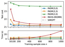
a. Basic Results. In Figure 1a, we report comparison results with the training sample size $n$ increasing from 50 to 1000. For a fair comparison, we set the PA function class with $(K_{1},K_{2})=(3,0)$ as the regression model in PO-PA, which contains the true model $\overline{Y}(\cdot)$; the parameters of the PA regression model are estimated by solving the corresponding ERM problem via the enhanced SMM algorithm with the same hyperparameter selection procedure as PADR methods. We also implement the quadratic DR and cubic DR as the generalized LDRs, denoted by GLDR-2 and GLDR-3 respectively, the running time of which is less than 0.5 seconds and thus is omitted.

(a) Basic Results            

(b) Enhanced SMM with Different $\varepsilon$-Strategies     

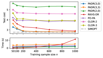
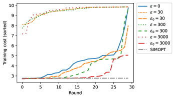
Unconstrained Newsvendor Problem: Basic Results We also test the performance of PO-L and LDR in this instance, whose costs (around 14 and 9, respectively) are excluded in (a) for readability. In (b), solid and dotted lines represent constant-$\varepsilon$ strategies; dashed lines represent shrinking-$\varepsilon$ strategies with $T_{0}=3$ and $\varepsilon_{1}=0$.

The costs of PADR(3,0) and PADR(3,3) converge to SIMOPT because the optimal DR in this case is a max-affine function with three pieces, and thus PADR(3,0) and PADR(3,3) have no approximation error in principle. The RKHS-DR method converges slower than PADR(3,0) and PADR(3,3); moreover, its performance with $n=1000$ is slightly worse than that of PADR(3,0) with $n=400$. For PO-PA, given the observation that the prediction model provided by the enhanced SMM algorithm is quite close to the true model $\overline{Y}(\cdot)$, we conjecture that its gap to SIMOPT is mainly due to inconsistency between the prediction loss and Newsvendor cost with imbalanced $c_{b}$ and $c_{h}$. This phenomenon is more evident from the comparison between LDR and PO-L, the two methods with misspecified models. The training time of RKHS-DR grows roughly exponentially with respect to the sample size, whereas that of PA-related methods is quite stable and significantly shorter when $n=1000$, which can be mainly credited to the sampling strategy used in the enhanced SMM algorithm. The numerical results with the parameter ratio $c_{b}:c_{h}$ varying from 1:9 to 9:1 exhibit similar patterns and thus are omitted.

Figure 1b displays sorted training cost curves of PADR(3,3) provided by the enhanced SMM with constant-$\varepsilon$ and shrinking-$\varepsilon$ strategies over 30 rounds. The shrinking-$\varepsilon$ strategy significantly improves the performance of the algorithm compared to the constant-$\varepsilon$ strategy, which typically does not reach satisfactory convergence within 10 iterations. This indicates that despite the theoretical convergence of the algorithm to global optimality with sufficiently large $\varepsilon$, it needs to engage with a huge number of index mappings when the sample size is large and thus can hardly make a valid update in each iteration. In contrast, the shrinking-$\varepsilon$ strategy with $\varepsilon_{0}=3000$ approximately attains the optimal value in 18 rounds. The significant efficiency improvement is because the shrinking-$\varepsilon$ strategy enables flexible adjustments of iterate points at early iterations as a warm start and afterward accelerates the convergence by ensuring valid updates with $\varepsilon=0$.

b. Varying Feature Dimensions. We study the effect of the feature dimension $p$ on the performance of PADR methods under sparse and dense demand models $\overline{Y}$ following the settings in Bertsimas and Koduri (2021) and report the results in Figure 1d.

(c) Sparse Demand Model            

(d) Dense Demand Model             

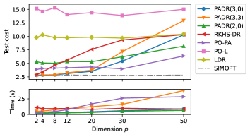
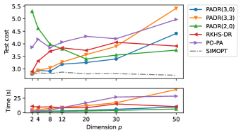
Unconstrained Newsvendor Problem with Varying Feature Dimensions We also test the performance of PO-L and LDR under dense demand models, whose costs (decreasing from 15 to 5 and 9 to 4, respectively) are excluded in (b) for readability.

In the sparse case, only the first two components of $X$ contribute to $\overline{Y}$ following the demand model (12); in the dense case, we replace $X_{1}$ in (12) with the average of the first half of the features $\frac{2}{p}\sum_{i=1}^{p/2}X_{i}$ and $X_{2}$ with the average of the other half. Figure 1d implies that PADR and PO-PA are generally more robust to redundant features than RKHS-DR in the sparse case, and that PADR performs better than RKHS-DR and PO-PA in the dense case. The performance of PADR(3,3) and PADR(3,0) deteriorates as $p$ increases due to the growing estimation error and optimization difficulty. The simpler PADR(2,0) performs more stable in both cases, despite the existence of an approximation error.

c. Nonlinearity in Demand Model. We study the effect of nonlinearity in the demand model (12) with varying $k$ and report results in Figure 1f. It indicates that the performance of PADR(3,0), PADR(3,3), and PO-PA is irrelevant to the nonlinearity level of the demand model, whereas that of PADR(2,0) and RKHS-DR deteriorates as the nonlinearity level increases.

(e) $p=2\phantom{xxxxxxx}$

(f) $p=20$            

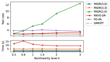
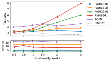
Unconstrained Newsvendor Problem with Varying Nonlinearity in Demand Model In (b), the demand model is of the dense type. We also test the performance of PO-L and LDR, whose costs are excluded for readability. When $p=2$, PO-L and LDR increase from 5 to 40 and 3 to 30, respectively; when $p=20$, PO-L and LDR increase from 4 to 16 and 3 to 13, respectively.

Besides the piecewise affine demand model (12), we also test the performance of the DR-based methods with another nonlinear demand model that includes a sine function to account for seasonality. The numerical results are provided in Appendix 12.

6.2 Constrained Newsvendor Problem

We next consider a two-product Newsvendor problem with a total inventory capacity $C_{0}$. Assume that the uncensored historical demand data is available. We denote the unit back-order cost, unit holding cost, and order decision by $c_{bi}$, $c_{hi}$, and $z_{i}$ respectively for product $i=1,2$. The capacity constraint is formulated as $z_{1}+z_{2}\leq C_{0}$. In this subsection, we set $(c_{b1},c_{h1},c_{b2},c_{h2})=(8,2,2,8)$, $C_{0}=60$, and the mean demand models for the two products as

$$\overline{Y}_{1}(X)=15X_{1}-5X_{2}+30,\quad\overline{Y}_{2}(X)=15X_{1}+5X_{2}+30,$$

under which the probability that the constraint is active at the optimal decision is around 0.5. We compare PADR(2,2) with PO-L and the penalized RKHS-DR method from Bertsimas and Koduri (2021, Section 6.2).

Since DR-based methods may yield infeasible decisions, in Figure 1i we report the feasible frequency of decisions provided by PADR(2,2) and RKHS-DR. By projecting the decisions to the convex feasible region when needed, we report the test cost of the feasible decisions in Figure 1i.

(g) Basic Results

(h) Sparse Demand Model

(i) Dense Demand Model

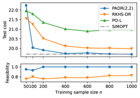
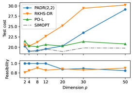
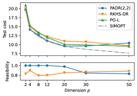
Newsvendor Problem with a Capacity Constraint

With the basic demand model, PADR(2,2) converges to SIMOPT and attains 100% feasibility when $n\geq 200$. In comparison, RKHS-DR and PO-L display notable gaps to SIMOPT, and the feasible frequency of RKHS-DR is only around 80%. Figures 1h and 1i display numerical results with varying feature dimensions. In the sparse case, PO-L is markedly better than the other two methods when $p=50$, indicating that regularization for sparsity is needed for learning PADR and RKHS-DR. In the dense case, PADR(2,2) performs the best except when $p=50$.

6.3 Nonconvex Newsvendor Problem

In this section, we consider two variations of the Newsvendor problem by adding a concave cost $C(z)$ in the objective or as a constraint. The cost $C(z)$ added in the objective can be interpreted as the capacity acquisition cost (Atamtürk and Hochbaum 2001); it also can be restricted in a constraint as a resource limitation. In the following experiments, we set the concave cost as

$$C(z)=\min\{z,0.6z+0.8,0.4z+15.6\},$$

and then both two variant problems of interest are nonconvex. We compare the PADR methods with RKHS-DR and use the deterministic MM algorithm to solve the nonconvex ERM problem for learning RKHS-DR, referred to as RKHS-DR(MM). The baseline SIMOPT is computed by solving simulated nonconvex problems via a solver of mix-integer linear programming.

a. Nonconvex Objective. We first consider a generalized single-product Newsvendor with $(c_{b},c_{h})=(5,5)$ and $C(z)$ added in the objective of (11). The numerical results in Figure 1l indicate that PADR(3,0) performs the best in almost all the settings, which is consistent with the convex case in Section 6.1; moreover, the gap between PADR(3,0) and RKHS-DR(MM) in the sparse case with $p=50$ is much more significant.

(j) Basic Results

(k) Sparse Demand Model

(l) Dense Demand Model

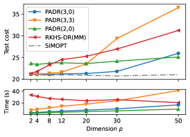
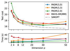
Newsvendor Problem with a Nonconvex Objective

b. Nonconvex Constraint. We next consider the 2-product Newsvendor problem given in Section 6.2 with parameters $(c_{b1},c_{h1},c_{b2},c_{h2})=(7,7,3,3)$ and the replacement of the convex constraint by $C(z_{1})+C(z_{2})\leq C_{0}$. We set $C_{0}=50$ to keep the same active probability for the constraint. Since the projection of infeasible decisions to the nonconvex feasible region may not yield meaningful solutions, we only report the average test cost of feasible decisions in Figure 1o, with a careful hyperparameter selection to ensure high feasible frequencies.

(m) Basic Results

(n) Sparse Demand Model

(o) Dense Demand Model

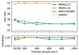
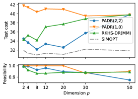
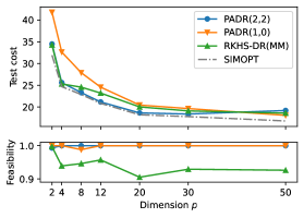
Newsvendor Problem with a Nonconvex Constraint In (b) and (c) with $p=50$, RKHS-DR(MM) takes more than 500 seconds on average, while PADR(2,2) takes less than 200 seconds.

For the problem with the basic demand model (12), PADR(2,2) performs comparably with RKHS-DR(MM), with a notable gap to SIMOPT. Figures 1n and 1o indicate the superiority of PADR(2,2) over the other two methods under both sparse and dense demand models with varying feature dimensions. It’s also worth noting that the simpler PADR(1,0) (equivalent to LDR), with poor performance in general, performs comparably well with the others in the high-dimensional case. It is more difficult to obtain feasible solutions for cases with sparse models than those with dense models; moreover, with sparse models, PADR(1,0) is more likely to produce feasible solutions than the others.

Finally, we also conduct experiments on constrained Newsvendor problems in Sections 6.2 and 6.3 with multiple $C_{0}$ values and Newsvendor cost parameters. The numerical results exhibit similar patterns and thus are omitted.

7 Conclusion

We propose the PADR-based ERM method together with the enhanced SMM algorithm to solve a broad class of SP problems with covariate information. For our PADR-based ERM framework, we provide the approximation bound of the PA function class and further establish the nonasymptotic consistency result for unconstrained problems and the asymptotic consistency result for deterministic-constrained ones. To solve the ERM problem with a composite DC structure, we develop the enhanced SMM algorithm by combining enhanced $\varepsilon$-active surrogation with sequential sampling. We provide the asymptotic convergence of the enhanced SMM algorithm to composite strong d-stationarity, and the nonasymptotic convergence to d-stationarity via the error-bound analysis. Numerical experiments indicate the superiority of our method over PO methods and prominent DR-based methods in the Newsvendor problem regarding the test cost, computational time, and robustness to feature dimensions and nonlinearity of the underlying dependency. In conclusion, the PADR is a favorable hypothesis class for DR-based ERM methods, supported by theoretical consistency, algorithmic convergence, and computational efficiency for solving SP with covariate information. Extensions of the PADR-based ERM framework for more complicated SP problems are deserved to be explored in the future, such as problems with chance constraints or endogenous random variables, which necessitate a further investigation of model construction, consistency analysis, and data-driven algorithmic development for problems with more complex composite structures.

.15.18.

Supplementary Material for

Data-driven Piecewise Affine Decision Rules for Stochastic Programming with Covariate Information

8 Proofs of Theoretical Consistency Results in Section 2

8.1 Proof of Proposition 2.1

The idea of the proof is to construct an interpolation PA function to a set of points related to the target function $f_{0}$ and a cover of the set $\mathcal{X}$. The structure of the interpolation function is motivated by Siahkamari et al. (2020) but with a different parameter, which ensures the Lipschitz continuity of the function with modulus independent of the approximation accuracy.

Proof 8.1

Proof of Proposition 2.1. It suffices to justify the bound when $d=1$. For $\epsilon>0$ satisfying $(\sqrt{p}\bar{X}/\epsilon)\geq 1$, we first construct a $(2\epsilon/\sqrt{p})$-grid of the cube $\bar{\mathcal{X}}\coloneqq[-\bar{X},\bar{X}]^{p}$, which is also an $\epsilon\text{-cover}$ of $\bar{\mathcal{X}}$ with $\ell_{2}$-norm, denoted by $\widehat{\mathcal{C}}_{2}(\epsilon;\bar{\mathcal{X}})$. Let $d_{\min}\coloneqq\underset{\widehat{x}_{1},\widehat{x}_{2}\in\widehat{\mathcal{C}}_{2}(\epsilon;\bar{\mathcal{X}}),\,\widehat{x}_{1}\neq\widehat{x}_{2}}{\min}\left\lVert\widehat{x}_{1}-\widehat{x}_{2}\right\rVert=\frac{2\epsilon}{\sqrt{p}}$. The cardinality of $\widehat{\mathcal{C}}_{2}(\epsilon;\bar{\mathcal{X}})$ satisfies

$$\left(\frac{\sqrt{p}\bar{X}}{\epsilon}\right)^{p}\leq\left\lvert\widehat{\mathcal{C}}_{2}(\epsilon;\bar{\mathcal{X}})\right\rvert\leq\left(\frac{\sqrt{p}\bar{X}}{\epsilon}+1\right)^{p}\leq\left(\frac{2\sqrt{p}\bar{X}}{\epsilon}\right)^{p}.$$

Given $f_{0}\in\mathcal{F}_{L_{0},M_{0}}$, by McShane (1934, Theorem 1), we can extend $f_{0}$ to an $L_{0}$-Lipschitz function $\bar{f}_{0}:\bar{\mathcal{X}}\rightarrow\mathbb{R}$ satisfying $\left\lVert\bar{f}_{0}\right\rVert_{\infty}\leq M_{0}$ and $\bar{f}_{0}(x)=f_{0}(x)$ for any $x\in\mathcal{X}$. Next, we construct a piecewise affine interpolation function to a set of points $\{(\widehat{x},\bar{f}_{0}(\widehat{x}))\mid\widehat{x}\in\widehat{\mathcal{C}}_{2}(\epsilon;\bar{\mathcal{X}})\}$:

$$f_{\widehat{\mathcal{C}}}(x)\coloneqq \max_{\widehat{x}\in\widehat{\mathcal{C}}_{2}(\epsilon;\bar{\mathcal{X}})}\left\{C\widehat{x}^{\top}(x-\widehat{x})+\frac{C}{2}\left\lVert\widehat{x}\right\rVert^{2}+\frac{1}{2}\bar{f}_{0}(\widehat{x})\right\}-\max_{\widehat{x}\in\widehat{\mathcal{C}}_{2}(\epsilon;\bar{\mathcal{X}})}\left\{C\widehat{x}^{\top}(x-\widehat{x})+\frac{C}{2}\left\lVert\widehat{x}\right\rVert^{2}-\frac{1}{2}\bar{f}_{0}(\widehat{x})\right\},$$ (13)

where $C\coloneqq L_{0}/d_{\min}=L_{0}\sqrt{p}/(2\epsilon)$. The function $f_{\widehat{\mathcal{C}}}$ indeed interpolates $\{(\widehat{x},\bar{f}_{0}(\widehat{x})):\widehat{x}\in\widehat{\mathcal{C}}_{2}(\epsilon;\bar{\mathcal{X}})\}$. Specifically, for any $\widehat{y}\in\widehat{\mathcal{C}}_{2}(\epsilon;\bar{\mathcal{X}})$,

$$\max_{\widehat{x}\in\widehat{\mathcal{C}}_{2}(\epsilon;\bar{\mathcal{X}})}\left\{C\widehat{x}^{\top}(\widehat{y}-\widehat{x})+\frac{1}{2}C\left\lVert\widehat{x}\right\rVert^{2}+\frac{1}{2}\bar{f}_{0}(\widehat{x})\right\} =\max_{\widehat{x}\in\widehat{\mathcal{C}}_{2}(\epsilon;\bar{\mathcal{X}})}\left\{\frac{1}{2}C\left\lVert\widehat{y}\right\rVert^{2}-\frac{1}{2}C\left\lVert\widehat{x}-\widehat{y}\right\rVert^{2}+\frac{1}{2}\bar{f}_{0}(\widehat{x})\right\}$$

$$\leq\max_{\widehat{x}\in\widehat{\mathcal{C}}_{2}(\epsilon;\bar{\mathcal{X}})}\left\{\frac{1}{2}C\left\lVert\widehat{y}\right\rVert^{2}-\frac{1}{2}L_{0}\left\lVert\widehat{x}-\widehat{y}\right\rVert+\frac{1}{2}\bar{f}_{0}(\widehat{x})\right\}$$

$$\leq\max_{\widehat{x}\in\widehat{\mathcal{C}}_{2}(\epsilon;\bar{\mathcal{X}})}\left\{\frac{1}{2}C\left\lVert\widehat{y}\right\rVert^{2}-\frac{1}{2}\left\lvert\bar{f}_{0}(\widehat{x})-\bar{f}_{0}(\widehat{y})\right\rvert+\frac{1}{2}\bar{f}_{0}(\widehat{x})\right\}$$

$$\leq\frac{1}{2}C\left\lVert\widehat{y}\right\rVert^{2}+\frac{1}{2}\bar{f}_{0}(\widehat{y}),$$

where the first inequality holds since $C=L_{0}/d_{\min}\geq L_{0}/\left\lVert\widehat{x}-\widehat{y}\right\rVert$. Moreover, this upper bound is attained by taking $\widehat{x}=\widehat{y}$ in the max operator. Similarly, the value of the second max-affine component of $f_{\widehat{\mathcal{C}}}$ at $\widehat{y}$ is $\frac{1}{2}C\left\lVert\widehat{y}\right\rVert^{2}-\frac{1}{2}\bar{f}_{0}(\widehat{y})$. Hence, we obtain $f_{\widehat{\mathcal{C}}}(\widehat{y})=\bar{f}_{0}(\widehat{y})$, verifying the interpolation. With $K\coloneqq\left\lvert\widehat{\mathcal{C}}_{2}(\epsilon;\bar{\mathcal{X}})\right\rvert$, for any $\widehat{x}\in\widehat{\mathcal{C}}_{2}(\epsilon;\bar{\mathcal{X}})$, we obtain $\left\lVert C\widehat{x}\right\rVert_{\infty}\leq\frac{L_{0}\sqrt{p}}{2\epsilon}\bar{X}\leq\frac{L_{0}}{2}K^{1/p}$ and

$$\left\lvert-C\left\lVert\widehat{x}\right\rVert^{2}+\frac{1}{2}C\left\lVert\widehat{x}\right\rVert^{2}\pm\frac{1}{2}\bar{f}_{0}(\widehat{x})\right\rvert\leq\frac{1}{2}Cp\left\lVert\widehat{x}\right\rVert_{\infty}^{2}+\frac{1}{2}M_{0}\leq\frac{1}{4}pL_{0}\bar{X}K^{1/p}+\frac{1}{2}M_{0}.$$

Therefore, with $\mu\geq\max\left\{\frac{1}{2}L_{0}K^{1/p},\frac{1}{4}pL_{0}\bar{X}K^{1/p}+\frac{1}{2}M_{0}\right\}$, we have $f_{\widehat{\mathcal{C}}}\in{\mathcal{H}}_{\mu}^{K}$.

Note that for any $w\in\mathcal{X}$, there exists $\widehat{x}(w)\in\widehat{\mathcal{C}}_{2}(\epsilon;\bar{\mathcal{X}})$ such that $\left\lVert w-\widehat{x}(w)\right\rVert\leq\epsilon$ and $f_{\widehat{\mathcal{C}}}(\widehat{x}(w))=\bar{f}_{0}(\widehat{x}(w))$. We next show that $f_{\widehat{\mathcal{C}}}$ is Lipschitz continuous with modulus $(\sqrt{p}+2)L_{0}$, with which we obtain the desired inequality,

$$\begin{array}[]{ll}\displaystyle{\min_{f\in{\mathcal{H}}_{\mu}^{K}}}\max_{w\in\mathcal{X}}\left\lvert f(w)-f_{0}(w)\right\rvert&\leq\displaystyle{\max_{w\in\mathcal{X}}}\left\lvert f_{\widehat{\mathcal{C}}}(w)-f_{0}(w)\right\rvert\leq\displaystyle{\max_{w\in\mathcal{X}}}\left\{\left\lvert f_{\widehat{\mathcal{C}}}(w)-f_{\widehat{\mathcal{C}}}(\widehat{x}(w))\right\rvert+\left\lvert\bar{f}_{0}(\widehat{x}(w))-\bar{f}_{0}(w)\right\rvert\right\}\\ &\leq 2(p^{1/2}+3)p^{1/2}L_{0}\bar{X}K^{-1/p},\end{array}$$

where the last inequality follows from the Lipschitz continuity of $f_{\widehat{\mathcal{C}}}$ and $\bar{f}_{0}$ and the relation $K\leq(2\sqrt{p}\bar{X}/\epsilon)^{p}$. For any $x\in\bar{\mathcal{X}}$, let

$$\begin{array}[]{ll}&\mathcal{A}_{1}(x)\coloneqq\displaystyle{\mathop{\arg\max}_{\widehat{x}\in\widehat{\mathcal{C}}_{2}(\epsilon;\bar{\mathcal{X}})}}\left\{C\widehat{x}^{\top}(x-\widehat{x})+\frac{C}{2}\left\lVert\widehat{x}\right\rVert^{2}+\frac{1}{2}\bar{f}_{0}(\widehat{x})\right\},\\ &\mathcal{A}_{2}(x)\coloneqq\displaystyle{\mathop{\arg\max}_{\widehat{x}\in\widehat{\mathcal{C}}_{2}(\epsilon;\bar{\mathcal{X}})}}\left\{C\widehat{x}^{\top}(x-\widehat{x})+\frac{C}{2}\left\lVert\widehat{x}\right\rVert^{2}-\frac{1}{2}\bar{f}_{0}(\widehat{x})\right\}.\end{array}$$

It suffices to show that $\left\lVert C(\widehat{x}_{1}^{*}-\widehat{x}_{2}^{*})\right\rVert\leq(\sqrt{p}+2)L_{0}$ for any $\widehat{x}_{1}^{*}\in\mathcal{A}_{1}(x)$ and $\widehat{x}_{2}^{*}\in\mathcal{A}_{2}(x)$. Let $\widehat{x}\in\widehat{\mathcal{C}}_{2}(\epsilon;\bar{\mathcal{X}})$ satisfy $\left\lVert x-\widehat{x}\right\rVert\leq\epsilon$. For any $\widehat{y}\in\widehat{\mathcal{C}}_{2}(\epsilon;\bar{\mathcal{X}})$ satisfying $\left\lVert x-\widehat{y}\right\rVert>\frac{\sqrt{p}+2}{\sqrt{p}}\epsilon$, we have that

$$C\widehat{y}^{\top}(x-\widehat{y})+\frac{1}{2}C\left\lVert\widehat{y}\right\rVert^{2}+\frac{1}{2}\bar{f}_{0}(\widehat{y}) =\frac{1}{2}\left[C\left\lVert x\right\rVert^{2}-C\left\lVert x-\widehat{y}\right\rVert^{2}+\bar{f}_{0}(\widehat{y})\right]$$

$$=\frac{1}{2}\left[\bar{f}_{0}(\widehat{y})-\bar{f}_{0}(x)-C\left\lVert x-\widehat{y}\right\rVert^{2}\right]+\frac{1}{2}\left[C\left\lVert x\right\rVert^{2}+\bar{f}_{0}(x)\right]$$

$$\leq\frac{1}{2}\left[L_{0}\left\lVert x-\widehat{y}\right\rVert-\frac{\sqrt{p}L_{0}}{2\epsilon}\left\lVert x-\widehat{y}\right\rVert^{2}\right]+\frac{1}{2}\left[C\left\lVert x\right\rVert^{2}+\bar{f}_{0}(x)\right]$$

$$<\frac{1}{2}\left[L_{0}\cdot\frac{\sqrt{p}+2}{\sqrt{p}}\epsilon-\frac{\sqrt{p}L_{0}}{2\epsilon}\left(\frac{\sqrt{p}+2}{\sqrt{p}}\epsilon\right)^{2}\right]+\frac{1}{2}\left[C\left\lVert x\right\rVert^{2}+\bar{f}_{0}(x)\right]$$

$$=\frac{1}{2}\left[-L_{0}\cdot\epsilon-\frac{\sqrt{p}L_{0}}{2\epsilon}\epsilon^{2}\right]+\frac{1}{2}\left[C\left\lVert x\right\rVert^{2}+\bar{f}_{0}(x)\right]$$

$$\leq\frac{1}{2}\left[\bar{f}_{0}(\widehat{x})-\bar{f}_{0}(x)-C\left\lVert x-\widehat{x}\right\rVert^{2}\right]+\frac{1}{2}\left[C\left\lVert x\right\rVert^{2}+\bar{f}_{0}(x)\right]$$

$$=C\widehat{x}^{\top}(x-\widehat{x})+\frac{1}{2}C\left\lVert\widehat{x}\right\rVert^{2}+\frac{1}{2}\bar{f}_{0}(\widehat{x}),$$

where the second inequality is derived by the strict monotonicity of the quadratic function $t\mapsto L_{0}t-\frac{\sqrt{p}L_{0}}{2\epsilon}t^{2}$ on $[\epsilon/\sqrt{p},+\infty)$. The above result shows $\left\lVert\widehat{x}_{1}^{*}-x\right\rVert\leq\frac{\sqrt{p}+2}{\sqrt{p}}\epsilon$ for all $\widehat{x}_{1}^{*}\in\mathcal{A}_{1}(x)$. Similarly, we have $\left\lVert\widehat{x}_{2}^{*}-x\right\rVert\leq\frac{\sqrt{p}+2}{\sqrt{p}}\epsilon$ for all $\widehat{x}_{2}^{*}\in\mathcal{A}_{2}(x)$. It follows that

$$\left\lVert C(\widehat{x}_{1}^{*}-\widehat{x}_{2}^{*})\right\rVert\leq C\left\lVert\widehat{x}_{1}^{*}-x\right\rVert+C\left\lVert\widehat{x}_{2}^{*}-x\right\rVert\leq 2\frac{\sqrt{p}L_{0}}{2\epsilon}\cdot\frac{\sqrt{p}+2}{\sqrt{p}}\epsilon\leq(\sqrt{p}+2)L_{0},$$

which completes the proof.∎

8.2 Proofs of Proposition 2.2 and Theorem 2.3

8.2.1 Preliminaries on Rademacher Complexity.

We start with a brief introduction to the Rademacher complexity, which is utilized to quantify the generalization error. The empirical Rademacher complexity of a function class is defined as follows.

Definition 8.2

Let $\Phi$ be a class of functions mapping from $\mathcal{U}$ to $\mathbb{R}$ and $S_{N}=\{u^{s}\}_{s=1}^{N}\subseteq\mathcal{U}$ be a sample set of size $N$. Then the empirical Rademacher complexity of $\Phi$ with respect to $S_{N}$ is defined as

$$\widehat{\mathcal{R}}_{S_{N}}(\Phi)\coloneqq\mathbb{E}_{\boldsymbol{\sigma}}\left[\sup_{\phi\in\Phi}\frac{1}{N}\sum_{s=1}^{N}\sigma_{s}\phi(u^{s})\right],$$

where ${\boldsymbol{\sigma}}=(\sigma_{1},\dots,\sigma_{N})^{\top}$ is a uniform random vector taking values in $\{-1,+1\}^{N}$.

The Rademacher complexity of $\Phi$ is defined as the expectation of the empirical Rademacher complexity over all samples of size $N$ drawn from the underlying distribution:

$$\mathcal{R}_{N}(\Phi)\coloneqq\mathbb{E}_{S_{N}}[\widehat{\mathcal{R}}_{S_{N}}(\Phi)].$$

It captures the richness of the class $\Phi$ by measuring the degree to which a hypothesis set can fit random noise. The following lemma quantifies the Rademacher complexity of a class of parametric functions, which is generalized from Ermoliev and Norkin (2013, Lemma B.2) with minor modifications made to accommodate the developments in this paper.

Lemma 8.3

Let $\widehat{\Phi}\coloneqq\{\phi(\cdot;\theta):\mathcal{U}\rightarrow\mathbb{R}\mid\theta\in\Theta\}$ be a class of functions parameterized by vectors in a compact set $\Theta\subseteq\mathbb{R}^{q}$ with $\max_{\theta\in\Theta}\left\lVert\theta\right\rVert_{\infty}=\mu$. Suppose that there exist $M_{\widehat{\Phi}}>0$ and $L_{\widehat{\Phi}}>0$ such that $\max_{\theta\in\Theta}\left\lVert\phi(\cdot;\theta)\right\rVert_{\infty}\leq M_{\widehat{\Phi}}$ and $\left\lVert\phi(\cdot;\theta_{1})-\phi(\cdot;\theta_{2})\right\rVert_{\infty}\leq L_{\widehat{\Phi}}\left\lVert\theta_{1}-\theta_{2}\right\rVert$ for any $\theta_{1},\theta_{2}\in\Theta$. Then

$$\mathcal{R}_{N}(\widehat{\Phi})\leq\frac{2\mu L_{\widehat{\Phi}}\sqrt{q}}{N}+M_{\widehat{\Phi}}\sqrt{\frac{q\log N}{N}}.$$

Proof 8.4

Proof of Lemma 8.3 Given a sample set $S_{N}=\{u^{s}\}_{s=1}^{N}$ of size $N$, following the proof of Ermoliev and Norkin (2013, Lemma B.2), we derive that for any $\epsilon\in(0,2\mu]$,

$$\widehat{\mathcal{R}}_{S_{N}}(\widehat{\Phi})\leq L_{\widehat{\Phi}}\sqrt{q}\epsilon+M_{\widehat{\Phi}}\sqrt{\frac{2q\log(2\mu/\epsilon)}{N}}.$$

By setting $\epsilon=2\mu/N$ and taking expectation over $S_{N}$, we obtain the desired upper bound.∎

The following lemma gives the generalization bound based on the Rademacher complexity.

Lemma 8.5 (Mohri et al. (2018), Theorem 3.3)

Let $\Phi$ be a function class mapping from $\mathcal{U}$ to $[-M,M]$. Then for any $\delta>0$, with probability at least $1-\delta$ over the draw of an independently and identically distributed (i.i.d.) sample $S_{N}$ of size $N$, the following holds true for all $\phi\in\Phi$:

$$\mathbb{E}[\phi(\tilde{u})]\leq\frac{1}{N}\sum_{s=1}^{N}\phi(u^{s})+2{\mathcal{R}}_{N}(\Phi)+\sqrt{2}M\sqrt{\frac{\log(1/\delta)}{N}}.$$

8.2.2 Proofs of Proposition 2.2 and Theorem 2.3.

Proof 8.6

Proof of Proposition 2.2. We first quantify the Rademacher complexity of the composite function class $\Phi_{{\mathcal{H}}_{\mu}^{K}}\coloneqq\left\{\phi:\mathcal{X}\times\mathcal{Y}\rightarrow\mathbb{R}\mid\phi(x,y)=\varphi({f(x)};{y}),\,f\in{\mathcal{H}}_{\mu}^{K}\right\}$. Notice that any function in $\Phi_{{\mathcal{H}}_{\mu}^{K}}$ is parameterized by some $\theta\in[-\mu,\mu]^{2dK(p+1)}$. For any $(x,y)\in\mathcal{X}\times\mathcal{Y}$ and $\theta_{1},\theta_{2}\in[-\mu,\mu]^{2dK(p+1)}$,

$$\left\lvert\varphi(f(x;\theta_{1});y)-\varphi(f(x;\theta_{2});y)\right\rvert\leq L_{\varphi}\left\lVert f(x;\theta_{1})-f(x;\theta_{2})\right\rVert\leq 2L_{\varphi}\sqrt{p\bar{X}^{2}+1}\left\lVert\theta_{1}-\theta_{2}\right\rVert,$$

where the second inequality follows from Assumption (A2). Moreover, for any $f\in{\mathcal{H}}_{\mu}^{K}$,

$$\left\lvert\varphi(f(x);y)\right\rvert\leq\left\lvert\varphi(z_{0};y)\right\rvert+\left\lvert\varphi(f(x);y)-\varphi(z_{0};y)\right\rvert\leq C_{\varphi}+L_{\varphi}\left\lVert f(x)-z_{0}\right\rVert\leq M_{\mu}.$$ (14)

Therefore, by Lemma 8.3, we deduce

$$\mathcal{R}_{n}(\Phi_{{\mathcal{H}}_{\mu}^{K}})\leq\frac{4\mu L_{\varphi}\sqrt{2dK(p+1)(p\bar{X}^{2}+1)}}{n}+M_{\mu}\sqrt{\frac{2dK(p+1)\log n}{n}}.$$ (15)

Now we prove the uniform generalization bound. By Lemma 8.5 and the inequality (14), with probability at least $1-\delta/2$,

$$\max_{\phi\in\Phi_{{\mathcal{H}}_{\mu}^{K}}}\left(\mathbb{E}_{X,Y}\phi(X,Y)-\frac{1}{n}\sum_{s=1}^{n}\phi(x^{s},y^{s})\right)\leq 2{\mathcal{R}}_{n}(\Phi_{{\mathcal{H}}_{\mu}^{K}})+\sqrt{2}M_{\mu}\sqrt{\frac{\log(2/\delta)}{n}}.$$

For $\Phi_{{\mathcal{H}}_{\mu}^{K}}^{-}\coloneqq\{-\phi:\phi\in\Phi_{{\mathcal{H}}_{\mu}^{K}}\}$, we have ${\mathcal{R}}_{n}(\Phi_{{\mathcal{H}}_{\mu}^{K}}^{-})={\mathcal{R}}_{n}(\Phi_{{\mathcal{H}}_{\mu}^{K}})$. Therefore, by applying Lemma 8.5 again to $\Phi_{{\mathcal{H}}_{\mu}^{K}}^{-}$ and using the union bound, we derive that with probability at least $1-\delta$,

$$\max_{f\in{\mathcal{H}}_{\mu}^{K}}\left\lvert R(f)-\widehat{R}_{S}(f)\right\rvert\leq 2\mathcal{R}_{n}(\Phi_{{\mathcal{H}}_{\mu}^{K}})+\sqrt{2}M_{\mu}\sqrt{\frac{\log(2/\delta)}{n}}.$$ (16)

Finally, by combining (15) and (16), we complete the proof.∎

Proof 8.7

Proof of Theorem 2.3. Let $f^{*}_{{\mathcal{H}}_{\mu}^{K}}$ denote the optimal solution to problem (2) restricted to ${\mathcal{H}}_{\mu}^{K}$. Following the excess risk decomposition (7), we derive the excess risk bound by bounding the approximation and estimation errors respectively. With $f_{app}\in\mathop{\arg\min}_{f\in{\mathcal{H}}_{\mu}^{K}}\left\lVert f-f^{*}\right\rVert_{\infty}$, the approximation error can be bounded as follows:

$$R(f^{*}_{{\mathcal{H}}_{\mu}^{K}})-\min_{f\in\mathcal{F}}R(f) \leq R(f_{app})-R(f^{*})$$

$$=\mathbb{E}_{X,Y}\left[\varphi({f_{app}(X)};{Y})-\varphi({f^{*}(X)};{Y})\right]$$

$$\leq L_{\varphi}\sup_{x\in\mathcal{X}}\left\lVert f_{app}(x)-f^{*}(x)\right\rVert_{2}$$

$$\leq 2L_{\varphi}\sqrt{d}(p^{1/2}+3)p^{1/2}L_{z}\bar{X}K^{-1/p},$$

where the last inequality follows from Proposition 2.1. For the estimation error, we have

$$R(f^{*}_{S,{\mathcal{H}}_{\mu}^{K}})-R(f^{*}_{{\mathcal{H}}_{\mu}^{K}}) =R(f^{*}_{S,{\mathcal{H}}_{\mu}^{K}})-\widehat{R}_{S}(f^{*}_{S,{\mathcal{H}}_{\mu}^{K}})+\widehat{R}_{S}(f^{*}_{S,{\mathcal{H}}_{\mu}^{K}})-R(f^{*}_{{\mathcal{H}}_{\mu}^{K}})$$

$$\leq R(f^{*}_{S,{\mathcal{H}}_{\mu}^{K}})-\widehat{R}_{S}(f^{*}_{S,{\mathcal{H}}_{\mu}^{K}})+\widehat{R}_{S}(f^{*}_{{\mathcal{H}}_{\mu}^{K}})-R(f^{*}_{{\mathcal{H}}_{\mu}^{K}})$$

$$\leq 2\left(\max_{f\in{\mathcal{H}}_{\mu}^{K}}\,|R(f)-\widehat{R}_{S}(f)|\right).$$

By Proposition 2.2, with probability at least $1-\delta$, we have

$$R(f^{*}_{S,{\mathcal{H}}_{\mu}^{K}})-R(f^{*}_{{\mathcal{H}}_{\mu}^{K}})\leq\frac{16\mu L_{\varphi}\sqrt{2dK(p+1)(p\bar{X}^{2}+1)}}{n}+4M_{\mu}\sqrt{\frac{2dK(p+1)\log n}{n}}+2\sqrt{2}M_{\mu}\sqrt{\frac{\log(2/\delta)}{n}}.$$

By combining these two error bounds, we obtain the desired inequality. ∎

9 Surrogation Construction of $F(\cdot;\xi)$ for Case 1 to Case 3

In this section, we first illustrate the construction of upper surrogation functions of $F(\cdot;\xi)\coloneqq\varphi(f(\cdot;\xi);\xi)$ for Case 1 to Case 3, which are directionally differentiable and satisfy the first three properties in Assumption (B1). Then we show in Claim 1 that $\widehat{F}^{\varepsilon}_{\min}(\theta;\theta^{\prime},\xi)\coloneqq\min_{I\in\mathcal{I}^{\varepsilon}(\theta^{\prime})}\widehat{F}(\theta;\theta^{\prime},\xi,I)$ with $\varepsilon\geq 0$ satisfies Condition (P5) for the three cases, which also validates Condition (P4) since $\widehat{F}^{\varepsilon}_{\min}(\cdot;\theta^{\prime},\xi)$ by construction is directionally differentiable and satisfies (P2).

Case 1:

since $f(\cdot;\xi)$ and $\varphi(\cdot;\xi)$ are both piecewise affine, the composite function $F(\cdot;\xi)=\varphi(f(\cdot;\xi);\xi)$ is also piecewise affine. Thus, following the surrogation construction of $f(\cdot;\xi)$ with the difference-of-max-affine representation in Section 3.1, we can construct the upper surrogation function of $F(\cdot;\xi)$, which satisfies the first three properties in Assumption (B1). Specifically, the first two properties clearly hold, and the bi-variate continuity of $\widehat{F}(\cdot;\cdot,\xi,I)$ is justified since given a fixed index mapping $I$, the surrogate of a PA function is independent of the reference point $\theta^{\prime}$.

Case 2:

by assumption, $\varphi(\cdot;\xi)$ can be written as $\varphi(\cdot;\xi)=\varphi^{\uparrow}(\cdot;\xi)+\varphi^{\downarrow}(\cdot;\xi)$, where $\varphi^{\uparrow}(\cdot;\xi)$ and $\varphi^{\downarrow}(\cdot;\xi)$ are nondecreasing and nonincreasing convex functions respectively, that is, for any $\theta_{1},\theta_{2}\in\Theta$ satisfying $\theta_{1}\leq\theta_{2}$ componentwisely, we have $\varphi^{\uparrow}(\theta_{2};\xi)\geq\varphi^{\uparrow}(\theta_{1};\xi)$ and $\varphi^{\downarrow}(\theta_{2};\xi)\leq\varphi^{\downarrow}(\theta_{1};\xi)$. With $I=(I_{1},I_{2})\in\mathcal{I}^{\varepsilon}(\theta^{\prime})$, the surrogation function of $F(\cdot;\xi)$ at $\theta^{\prime}$ is constructed as

$$\widehat{F}(\theta;\theta^{\prime},\xi,I)=\varphi^{\uparrow}(\widehat{f}(\theta;\xi,I_{2});\xi)+\varphi^{\downarrow}(\widecheck{f}(\theta;\xi,I_{1});\xi),$$

where $\widehat{f}(\theta;\xi,I_{2})$ and $\widecheck{f}(\theta;\xi,I_{1})$ are the upper and lower surrogation functions of $f(\theta,\xi)$ respectively. By monotonicity of $\varphi^{\uparrow}$ and $\varphi^{\downarrow}$, $\widehat{F}(\theta;\theta^{\prime},\xi,I)\geq\varphi^{\uparrow}(f(\theta;\xi);\xi)+\varphi^{\downarrow}(f(\theta;\xi);\xi)=F(\theta;\xi)$ for any $\theta\in\Theta$, and thus the majorizing condition (P2) holds. Moreover, $\widehat{F}(\cdot;\theta^{\prime},\xi,I)$ satisfies the convex condition (P3) since a nondecreasing convex function composite with a convex function and a nonincreasing convex function composite with a concave function are both convex. The touching condition (P1) clearly holds when $\varepsilon=0$. With a fixed index mapping $I$, $\widehat{F}(\cdot;\theta^{\prime},\xi,I)$ in this case is also independent of $\theta^{\prime}$, validating the bi-variate continuity of $\widehat{F}(\cdot;\cdot,\xi,I)$.

Case 3:

since $S$ is finite, for any $\xi\in S$, $\varphi(\cdot;\xi)$ is Lipschitz smooth with uniform modulus denoted by $L_{\nabla\varphi}$, and $f(\cdot;\xi)$ is Lipschitz continuous with uniform modulus $L_{f}\coloneqq 2\sqrt{\max_{s\in[n]}\left\lVert x^{s}\right\rVert^{2}+1}$. Then the surrogation function of $F(\cdot;\xi)$ at $\theta^{\prime}$ with $I=(I_{1},I_{2})\in\mathcal{I}^{\varepsilon}(\theta^{\prime})$ is constructed by surrogating the inner PA function according to componentwise signs of the gradient $\nabla\varphi(f(\theta^{\prime};\xi);\xi)$ as follows,

$$\widehat{F}(\theta;\theta^{\prime},\xi,I) =\max\{\nabla{\varphi}(f(\theta^{\prime};\xi);\xi),0\}^{\top}\widehat{f}(\theta;\xi,I_{2})-\max\{-\nabla{\varphi}(f(\theta^{\prime};\xi);\xi),0\}^{\top}\widecheck{f}(\theta;\xi,I_{1})$$

$$\phantom{=,}-\nabla{\varphi}(f(\theta^{\prime};\xi);\xi)^{\top}f(\theta^{\prime};\xi)+\varphi(f(\theta^{\prime};\xi);\xi)+\frac{1}{2}L_{\nabla\varphi}L_{f}^{2}\left\lVert\theta-\theta^{\prime}\right\rVert^{2}.$$

The convex condition (P3) holds evidently; the touching condition (P1) also holds when $\varepsilon=0$. The surrogate $\widehat{F}(\cdot;\cdot,\xi,I)$ is continuous on $\Theta\times\Theta$ since $\nabla\varphi(\cdot;\xi)$ is continuous. Based on the quadratic upper bound of a Lipschitz smooth function, the majorizing condition (P2) is verified as follows. Since $\varphi(\cdot;\xi)$ is $L_{\nabla\varphi}$-smooth, we have for any $z_{1},z_{2}\in\mathbb{R}^{d}$ that

$$\varphi(z_{1};\xi)\leq\varphi(z_{2};\xi)+\nabla\varphi(z_{2};\xi)^{\top}(z_{1}-z_{2})+\frac{L_{\nabla\varphi}}{2}\left\lVert z_{1}-z_{2}\right\rVert^{2}.$$

By setting $z_{1}=f(\theta;\xi)$ and $z_{2}=f(\theta^{\prime};\xi)$, we obtain that for any $I=(I_{1},I_{2})\in\mathcal{I}^{\varepsilon}(\theta^{\prime})$,

$$F(\theta;\xi) \leq F(\theta^{\prime};\xi)+\nabla\varphi(f(\theta^{\prime};\xi);\xi)^{\top}(f(\theta;\xi)-f(\theta^{\prime};\xi))+\frac{L_{\nabla\varphi}}{2}\left\lVert f(\theta;\xi)-f(\theta^{\prime};\xi)\right\rVert^{2}$$

$$\leq F(\theta^{\prime};\xi)+\max\{\nabla{\varphi}(f(\theta^{\prime};\xi);\xi),0\}^{\top}\widehat{f}(\theta;\xi,I_{2})$$

$$\phantom{\leq,}-\max\{-\nabla{\varphi}(f(\theta^{\prime};\xi);\xi),0\}^{\top}\widecheck{f}(\theta;\xi,I_{1})-\nabla\varphi(f(\theta^{\prime};\xi);\xi)^{\top}f(\theta^{\prime};\xi)+\frac{L_{\nabla\varphi}L_{f}^{2}}{2}\left\lVert\theta-\theta^{\prime}\right\rVert^{2}$$

$$=\widehat{F}(\theta;\theta^{\prime},\xi,I).$$

Claim 1

Let $\Theta$ be a compact set. Given $\varepsilon\geq 0$ and $\theta^{\prime}\in\Theta$, with the surrogation construction for Case 1 to Case 3, $\widehat{F}^{\varepsilon}_{\min}(\cdot;\theta^{\prime},\xi)$ satisfies Condition (P5) for any $\xi\in S$.

Proof 9.1

Proof of Claim 1. Since $\widehat{F}^{\varepsilon}_{\min}(\cdot;\theta^{\prime},\xi)$ also satisfies the majorizing condition (P2), by the compactness of $\Theta$, it suffices to show that

$$\widehat{\kappa}\coloneqq\limsup_{\theta\rightarrow\theta^{\prime},\theta\neq\theta^{\prime}}\frac{2(\widehat{F}^{\varepsilon}_{\min}(\theta;\theta^{\prime},\xi)-F(\theta;\xi))}{\left\lVert\theta-\theta^{\prime}\right\rVert^{2}}<+\infty.$$

For the piecewise affine function $f(\theta;\xi)\coloneqq g(\theta;\xi)-h(\theta;\xi)$, we have $\mathcal{I}_{h}^{0}(\theta)\subseteq\mathcal{I}_{h}^{\varepsilon}(\theta^{\prime})$ when $\theta\in\Theta$ is sufficiently close to $\theta^{\prime}$. It follows from (P2) that for any $\theta\in\Theta$ sufficiently close to $\theta^{\prime}$,

$$f(\theta;\xi)\leq\min_{I_{2}\in\mathcal{I}^{\varepsilon}_{h}(\theta^{\prime})}\widehat{f}(\theta;\xi,I_{2})\leq\min_{I_{2}\in\mathcal{I}_{h}^{0}(\theta)}\widehat{f}(\theta;\xi,I_{2})=f(\theta;\xi).$$

Therefore, by similar arguments for lower surrogation functions of $f(\cdot;\xi)$, we obtain that for any $\theta\in\Theta$ sufficiently close to $\theta^{\prime}$,

$$\min_{I_{2}\in\mathcal{I}^{\varepsilon}_{h}(\theta^{\prime})}\widehat{f}(\theta;\xi,I_{2})=f(\theta;\xi)=\max_{I_{1}\in\mathcal{I}^{\varepsilon}_{g}(\theta^{\prime})}\widecheck{f}(\theta;\xi,I_{1}).$$

For Case 1, since the objective is piecewise affine, we directly obtain $\widehat{\kappa}=0$. For Case 2, when $\theta$ is sufficiently close to $\theta^{\prime}$, we have

$$\widehat{F}^{\varepsilon}_{\min}(\theta;\theta^{\prime},\xi) \coloneqq\min_{(I_{1},I_{2})\in\mathcal{I}^{\varepsilon}(\theta^{\prime})}\widehat{F}(\theta;\theta^{\prime},\xi,(I_{1},I_{2}))$$

$$=\min_{I_{2}\in\mathcal{I}^{\varepsilon}_{h}(\theta^{\prime})}\varphi^{\uparrow}(\widehat{f}(\theta;\xi,I_{2});\xi)+\min_{I_{1}\in\mathcal{I}^{\varepsilon}_{g}(\theta^{\prime})}\varphi^{\downarrow}(\widecheck{f}(\theta;\xi,I_{1});\xi)$$

$$=\varphi^{\uparrow}\left(\min_{I_{2}\in\mathcal{I}^{\varepsilon}_{h}(\theta^{\prime})}\widehat{f}(\theta;\xi,I_{2});\xi\right)+\varphi^{\downarrow}\left(\max_{I_{1}\in\mathcal{I}^{\varepsilon}_{g}(\theta^{\prime})}\widecheck{f}(\theta;\xi,I_{1});\xi\right)$$

$$=F(\theta;\xi),$$

also implying $\widehat{\kappa}=0$. For Case 3, when $\theta$ is sufficiently close to $\theta^{\prime}$, we obtain

$$\widehat{F}^{\varepsilon}_{\min}(\theta;\theta^{\prime},\xi)=\nabla\varphi(f(\theta^{\prime};\xi);\xi)^{\top}(f(\theta;\xi)-f(\theta^{\prime};\xi))+\varphi(f(\theta^{\prime};\xi);\xi)+\frac{1}{2}L_{\nabla\varphi}L_{f}^{2}\left\lVert\theta-\theta^{\prime}\right\rVert^{2}.$$

Thus, by the second-order Taylor expansion of $\varphi(\cdot;\xi)$ at $f(\theta^{\prime};\xi)$, we obtain

$$\widehat{F}^{\varepsilon}_{\min}(\theta;\theta^{\prime},\xi)-F(\theta;\xi)=\frac{1}{2}L_{\nabla\varphi}L_{f}^{2}\left\lVert\theta-\theta^{\prime}\right\rVert^{2}-\frac{1}{2}v^{\top}\nabla^{2}\varphi(f(\theta^{\prime};\xi);\xi)v+o(\left\lVert v\right\rVert^{2}),$$

where $\left\lVert v\right\rVert=\left\lVert f(\theta;\xi)-f(\theta^{\prime};\xi)\right\rVert\leq L_{f}\left\lVert\theta-\theta^{\prime}\right\rVert$ by the Lipschitz continuity of $f$. By dividing the both sides by $\left\lVert\theta-\theta^{\prime}\right\rVert^{2}$ and taking $\limsup$ as $\theta\rightarrow\theta^{\prime}$ and $\theta\neq\theta^{\prime}$, we obtain that $\widehat{\kappa}$ is finite.∎

10 Details of Convergence Analysis in Section 4

10.1 Proof of Proposition 4.2 and Equivalence Between $\mathcal{S}^{d}_{\varepsilon,\rho}$ and $\mathcal{S}^{*}$

Proof 10.1

Proof of Proposition 4.2. Given $\varepsilon\geq 0$ and $\rho>0$, for any $\theta^{*}\in\mathcal{S}^{*}$ it holds that $\widehat{F}^{\varepsilon}_{\min}(\theta;\theta^{*})+\frac{\rho}{2}\left\lVert\theta-\theta^{*}\right\rVert^{2}>F(\theta)\geq F(\theta^{*})=\widehat{F}^{\varepsilon}_{\min}(\theta^{*};\theta^{*})$ for any $\theta\neq\theta^{*}$, showing $\theta^{*}\in\mathcal{S}^{d}_{\varepsilon,\rho}$ and thus $\mathcal{S}^{*}\subseteq\mathcal{S}^{d}_{\varepsilon,\rho}$. For any $\theta^{d}\in\mathcal{S}^{d}_{\varepsilon,\rho}$, from Condition (P4) and the first-order optimality condition, it follows that $F^{\prime}(\theta^{d};\theta-\theta^{d})=\widehat{F}^{\varepsilon}_{\min}(\cdot;\theta^{d})^{\prime}(\theta^{d};\theta-\theta^{d})\geq 0$ for all $\theta\in\Theta$, yielding $\theta^{d}\in\mathcal{S}^{d}$ and thus $\mathcal{S}^{d}_{\varepsilon,\rho}\subseteq\mathcal{S}^{d}$.

It remains to show $\mathcal{S}^{d}\subseteq\mathcal{S}^{d}_{0,\rho}$ for any $\rho>0$. Assume by contradiction that there exists $\theta^{d}\in\mathcal{S}^{d}\backslash\mathcal{S}^{d}_{0,\widehat{\rho}}$ for some $\widehat{\rho}>0$. Then there exist $\widehat{I}\in\mathcal{I}^{0}(\theta^{d})$ and $\widehat{\theta}(\neq\theta^{d})\in\Theta$ such that $\widehat{\theta}\in\mathop{\arg\min}_{\theta\in\Theta}\left\{\widehat{F}(\theta;\theta^{d},\widehat{I}\,)+\frac{\widehat{\rho}}{2}\left\lVert\theta-\theta^{d}\right\rVert^{2}\right\}$. By the strong convexity of the function $\theta\mapsto\widehat{F}(\theta;\theta^{d},\widehat{I}\,)+\frac{\widehat{\rho}}{2}\,\left\lVert\theta-\theta^{d}\right\rVert^{2}$, we have $\widehat{F}(\cdot;\theta^{d},\widehat{I})^{\prime}(\theta^{d};\widehat{\theta}-\theta^{d})<0$. Thus, there exists $t_{0}>0$ such that

$$F(\theta^{d}+t(\widehat{\theta}-\theta^{d}))\leq\widehat{F}(\theta^{d}+t(\widehat{\theta}-\theta^{d});\theta^{d},\widehat{I})<\widehat{F}(\theta^{d};\theta^{d},\widehat{I})=F(\theta^{d}),\quad\forall\,t\in(0,t_{0}],$$

where the equality holds by the touching condition (P1). This contradicts that $\theta^{d}$ is a d-stationary point. Therefore, we have $\mathcal{S}^{d}\subseteq\mathcal{S}^{d}_{0,\rho}$, which completes the proof.∎

As an extension, we show the equivalence between $\mathcal{S}^{d}_{\varepsilon,\rho}$ and $\mathcal{S}^{*}$ with sufficiently large $\varepsilon$ and suitable $\rho$ in Proposition 10.2. The following assumption is needed:

1. There exists $M_{\Delta}>0$ such that $F(\theta^{d})\geq\min_{\theta\in\Theta}F(\theta)+M_{\Delta}$ for any $\theta^{d}\in\mathcal{S}^{d}\backslash\mathcal{S}^{*}$.

The assumption is naturally satisfied when the outer function of $F$ is in Case 1 or Case 2. Specifically, from the proof of Claim 2 afterward, we see that in these two cases, $\Theta$ can be decomposed into finitely many convex regions, on each of which any d-stationary point $\theta^{d}\in\mathcal{S}^{d}$ is a minimizer of $F$ over that region. Since the number of such regions is finite, the function $F$ takes finitely many values on $\mathcal{S}^{d}$, verifying Assumption (B4). Discussions on the finite number of d-stationary values for more general nonconvex problems with piecewise and composite structures can be seen in Cui and Pang (2018).

Proposition 10.2

For problem (9) with $\max_{\theta\in\Theta}\left\lVert\theta\right\rVert_{\infty}=\mu$ and Assumption (B1) holding for the surrogate family $\{\widehat{F}(\cdot;\theta^{\prime},\xi,I)\}_{I\in\mathcal{I}^{\varepsilon}(\theta^{\prime})}$ of $F(\cdot;\xi)$ for each $\xi\in S$, the following statements hold:

1. With $\varphi$ in Case 1 or Case 2, $\mathcal{S}^{d}_{\varepsilon,\rho}=\mathcal{S}^{*}$ for any $\varepsilon\in[\varepsilon_{0},+\infty)$ and $\rho\in(0,\frac{M_{\Delta}}{2q\mu^{2}}]$, where $\varepsilon_{0}\coloneqq 2\mu\sqrt{q}\sqrt{\max_{s\in[n]}\left\lVert x^{s}\right\rVert^{2}+1}$, and $M_{\Delta}$ is the constant defined in (B4).

2. Suppose that Assumptions (B2) and (B4) additionally hold with $M_{\Delta}>2\kappa q\mu^{2}$. It holds that $\mathcal{S}^{d}_{\varepsilon,\rho}=\mathcal{S}^{*}$ for any $\varepsilon\in[\varepsilon_{0},+\infty)$ and $\rho\in(0,\frac{M_{\Delta}}{2q\mu^{2}}-\kappa]$.

Proof 10.3

Proof of Proposition 10.2. By Proposition 4.2, it suffices to prove the inclusion $\mathcal{S}^{d}_{\varepsilon,\rho}\subseteq\mathcal{S}^{*}$. Since the two max-affine components of $f(\cdot;\xi)$ for any $\xi\in S$ are Lipschitz continuous with modulus $L_{g,h}\coloneqq\sqrt{\max_{s\in[n]}\left\lVert x^{s}\right\rVert^{2}+1}$, we see that with $\varepsilon\geq\varepsilon_{0}=2L_{g,h}\sqrt{q}\mu$, the set $\mathcal{I}^{\varepsilon}(\theta^{\prime})$ contains all index mappings, that is, $\mathcal{I}^{\varepsilon}(\theta^{\prime})=\{(I_{1},I_{2})\mid I_{1}:S\rightarrow[K],I_{2}:S\rightarrow[K]\}$ for any $\theta^{\prime}\in\Theta$.

For the first statement, assume by contradiction that there exists $\widehat{\theta}^{d}\in\mathcal{S}^{d}_{\widehat{\varepsilon},\widehat{\rho}}\backslash\mathcal{S}^{*}$ for some $\widehat{\varepsilon}\in[\varepsilon_{0},+\infty)$ and $\widehat{\rho}\in(0,\frac{M_{\Delta}}{2q\mu^{2}}]$. Since the set $\mathcal{I}^{\widehat{\varepsilon}}(\widehat{\theta}^{d})$ contains all index mappings for the inner PA functions, by the surrogation construction for Case 1 and Case 2 in Appendix 9, for any $\theta^{*}\in\mathcal{S}^{*}$ there exists $I^{\widehat{\varepsilon}}\in\mathcal{I}^{\widehat{\varepsilon}}(\widehat{\theta}^{d})$ such that $\widehat{F}^{\widehat{\varepsilon}}_{\min}(\theta^{*};\widehat{\theta}^{d})=\widehat{F}(\theta^{*};\widehat{\theta}^{d},I^{\widehat{\varepsilon}})=\min_{\theta\in\Theta}F(\theta)$. It follows that

$$\widehat{F}^{\widehat{\varepsilon}}_{\min}(\theta^{*};\widehat{\theta}^{d})+\frac{\widehat{\rho}}{2}\,\big{\lVert}\,{\theta^{*}-\widehat{\theta}^{d}}\,\big{\rVert}^{2}\leq\min_{\theta\in\Theta}F(\theta)+M_{\Delta}\leq F(\widehat{\theta}^{d})=\widehat{F}^{\widehat{\varepsilon}}_{\min}(\widehat{\theta}^{d};\widehat{\theta}^{d}),$$

which contradicts $\widehat{\theta}^{d}\in\mathcal{S}^{d}_{\widehat{\varepsilon},\widehat{\rho}}$. For the second statement, in a similar way, assume that there exists $\widehat{\theta}^{d}\in\mathcal{S}^{d}_{\widehat{\varepsilon},\widehat{\rho}}\backslash\mathcal{S}^{*}$ for some $\widehat{\varepsilon}\in[\varepsilon_{0},+\infty)$ and $\widehat{\rho}\in(0,\frac{M_{\Delta}}{2q\mu^{2}}-\kappa]$. By Condition (P5), we have that for $\theta^{*}\in\mathcal{S}^{*}$,

$$\widehat{F}^{\widehat{\varepsilon}}_{\min}(\theta^{*};\widehat{\theta}^{d})+\frac{\widehat{\rho}}{2}\,\big{\lVert}\,{\theta^{*}-\widehat{\theta}^{d}}\,\big{\rVert}^{2}\leq F(\theta^{*})+\frac{\widehat{\rho}+\kappa}{2}\,\big{\lVert}\,{\theta^{*}-\widehat{\theta}^{d}}\,\big{\rVert}^{2}\leq\min_{\theta\in\Theta}F(\theta)+M_{\Delta}\leq F(\widehat{\theta}^{d}).$$

Again, it leads to a contradiction, which completes the proof.∎

10.2 Proof of Proposition 4.3

The following lemma from Deng and Gao (2021) is rephrased in our context for the proof of Proposition 4.3.

Lemma 10.4 (Deng and Gao (2021), Theorem 3.2)

Suppose that the stochastic function $\widehat{F}(\cdot;\theta^{\prime},\xi)$ is convex and Lipschitz continuous on $\Theta$ with modulus $L_{\widehat{F}}$ for any $\xi\in S$ and $\theta^{\prime}\in\Theta$, and that samples $\Xi_{N}\coloneqq\{\xi^{s}\}_{s=1}^{N}$ are i.i.d. generated from $S$. For $\eta>0$, denote $\theta^{\prime}_{+}\coloneqq\mathop{\arg\min}_{\theta\in\Theta}\left\{\frac{1}{N}\sum_{s=1}^{N}\widehat{F}(\theta;\theta^{\prime},\xi^{s})+\frac{\eta}{2}\left\lVert\theta-\theta^{\prime}\right\rVert^{2}\right\}$. Then it holds that

$$\left\lvert\mathbb{E}_{\Xi_{N}}\left[\frac{1}{N}\sum_{s=1}^{N}\widehat{F}(\theta^{\prime}_{+};\theta^{\prime},\xi^{s})-\mathbb{E}_{\widetilde{\xi}_{n}}\left[\widehat{F}(\theta^{\prime}_{+};\theta^{\prime},\widetilde{\xi}_{n})\right]\right]\right\rvert\leq\frac{2L_{\widehat{F}}^{2}}{\eta N}.$$

Proof 10.5

Proof of Proposition 4.3. Let $\widetilde{I}^{\varepsilon}_{\nu}$ be a random mapping uniformly drawn from $\mathcal{I}^{\varepsilon}(\theta^{\nu})$, $\{\widetilde{\xi}^{s}_{\nu}\}_{s=1}^{N_{\nu}}$ be random vectors independently and uniformly drawn from $S$, $\mathcal{G}_{\nu-1}$ denote the $\sigma$-algebra generated by all past samples $\{\{\widetilde{\xi}_{t}^{s}\}_{s=1}^{N_{t}}\}_{t=0}^{\nu-1}$ and mappings $\{\widetilde{I}^{\varepsilon}_{t}\}_{t=0}^{\nu-1}$, and $\mathcal{G}_{\nu-1}^{+}$ denote the $\sigma$-algebra generated by $\{\{\widetilde{\xi}_{t}^{s}\}_{s=1}^{N_{t}}\}_{t=0}^{\nu-1}$ and $\{\widetilde{I}^{\varepsilon}_{t}\}_{t=0}^{\nu}$. Given the current iterate $\theta^{\nu}$ and the index mapping $I^{\varepsilon}_{\nu}\in\mathcal{I}^{\varepsilon}(\theta^{\nu})$, by the definition of $P_{I^{\varepsilon}_{\nu}}^{\rho}(\cdot)$ in (10), we have

$$\min\left\{\widehat{F}(P^{\rho}_{I^{\varepsilon}_{\nu}}(\theta^{\nu});\theta^{\nu},I^{\varepsilon}_{\nu}),F(\theta^{\nu})\right\}+\frac{\rho}{2}\,\big{\lVert}\,{P^{\rho}_{I^{\varepsilon}_{\nu}}(\theta^{\nu})-\theta^{\nu}}\,\big{\rVert}^{2}\leq F(\theta^{\nu}).$$ (17)

With the notation $\mathbb{E}_{N_{\nu}}$ representing the expectation with respect to $\{\widetilde{\xi}_{\nu}^{s}\}_{s=1}^{N_{\nu}}$, by rearranging terms of (17) and taking the conditional expectation on both sides, we obtain that

$$\frac{\rho}{2}\mathbb{E}\left[\,\big{\lVert}\,{P^{\rho}_{\widetilde{I}^{\varepsilon}_{\nu}}(\theta^{\nu})-\theta^{\nu}}\,\big{\rVert}^{2}\,\middle|\,\mathcal{G}_{\nu-1}\right] \leq F(\theta^{\nu})-\mathbb{E}\left[\min\left\{\widehat{F}(P^{\rho}_{\widetilde{I}^{\varepsilon}_{\nu}}(\theta^{\nu});\theta^{\nu},\widetilde{I}^{\varepsilon}_{\nu}),F(\theta^{\nu})\right\}\,\middle|\,\mathcal{G}_{\nu-1}\right]$$

$$=\underbrace{F(\theta^{\nu})-W(\theta^{\nu})}_{\mathcal{E}_{1}^{\nu}}+\underbrace{W(\theta^{\nu})-\mathbb{E}\left[\min\left\{\widehat{F}(P^{\rho}_{\widetilde{I}^{\varepsilon}_{\nu}}(\theta^{\nu});\theta^{\nu},\widetilde{I}^{\varepsilon}_{\nu}),F(\theta^{\nu})\right\}\,\middle|\,\mathcal{G}_{\nu-1}\right]}_{\mathcal{E}_{2}^{\nu}},$$ (18)

where $W(\theta^{\nu})\coloneqq\mathbb{E}_{\widetilde{I}^{\varepsilon}_{\nu}}\left[\min\left\{\mathbb{E}_{N_{\nu}}\left[\widehat{F}_{N_{\nu}}({\theta}^{\nu+\frac{1}{2}};\theta^{\nu},\widetilde{I}^{\varepsilon}_{\nu})+\frac{\eta}{2}\,\big{\lVert}\,{{\theta}^{\nu+\frac{1}{2}}-\theta^{\nu}}\,\big{\rVert}^{2}\,\middle|\,\mathcal{G}_{\nu-1}^{+}\right],F(\theta^{\nu})\right\}\,\middle|\,\mathcal{G}_{\nu-1}\right]$.

From the update rule in Step 5 of Algorithm 1, we have $\widehat{F}_{N_{\nu}}({\theta}^{\nu+\frac{1}{2}};\theta^{\nu},I^{\varepsilon}_{\nu})+\frac{\eta}{2}\,\big{\lVert}\,{{\theta}^{\nu+\frac{1}{2}}-\theta^{\nu}}\,\big{\rVert}^{2}\geq F_{N_{\nu}}(\theta^{\nu+1})$ and $F_{N_{\nu}}(\theta^{\nu})\geq F_{N_{\nu}}(\theta^{\nu+1})$. It follows that

$$W(\theta^{\nu}) \geq\mathbb{E}_{\widetilde{I}^{\varepsilon}_{\nu}}\left[\min\left\{\mathbb{E}_{N_{\nu}}\left[F_{N_{\nu}}(\theta^{\nu+1})\mid\mathcal{G}_{\nu-1}^{+}\right],F(\theta^{\nu})\right\}\mid\mathcal{G}_{\nu-1}\right]=\mathbb{E}\left[F_{N\nu}(\theta^{\nu+1})\mid\mathcal{G}_{\nu-1}\right].$$

With $\Theta$ being a compact set, let $\max_{\theta\in\Theta}\left\lVert\theta\right\rVert_{\infty}=\mu$. Define

$$\widehat{\Phi}_{{\mathcal{H}}_{\mu}^{K}}\coloneqq\{\phi(\cdot;\theta):S\rightarrow\mathbb{R}\mid\phi(\xi;\theta)=\varphi(f(\theta;\xi);\xi),\,\xi\in S,f(\theta;\cdot)\in{\mathcal{H}}_{\mu}^{K},\theta\in\Theta\}.$$

From finiteness of $S$ and continuity of $\varphi(\cdot;\xi)$, it follows that for any $\phi\in\widehat{\Phi}_{{\mathcal{H}}_{\mu}^{K}}$, $\phi(\xi;\cdot)$ is Lipschitz continuous on the compact set $\Theta$ with uniform modulus, and that $\phi(\cdot;\theta)$ is uniformly bounded. Therefore, for the term $\mathcal{E}_{1}^{\nu}$, there exists a constant $C_{1}>0$ such that

$$\mathcal{E}_{1}^{\nu} \leq F(\theta^{\nu})-\mathbb{E}\left[F_{N_{\nu}}(\theta^{\nu+1})\mid\mathcal{G}_{\nu-1}\right]$$

$$=F(\theta^{\nu})-\mathbb{E}\left[F(\theta^{\nu+1})\mid\mathcal{G}_{\nu-1}\right]+\mathbb{E}\left[F(\theta^{\nu+1})\mid\mathcal{G}_{\nu-1}\right]-\mathbb{E}\left[F_{N_{\nu}}(\theta^{\nu+1})\mid\mathcal{G}_{\nu-1}\right]$$

$$\leq F(\theta^{\nu})-\mathbb{E}\left[F(\theta^{\nu+1})\mid\mathcal{G}_{\nu-1}\right]+\mathbb{E}\left[\sup_{\theta\in\Theta}\left\lvert F(\theta)-F_{N_{\nu}}(\theta)\right\rvert\,\middle|\,\mathcal{G}_{\nu-1}\right]$$

$$\leq F(\theta^{\nu})-\mathbb{E}\left[F(\theta^{\nu+1})\mid\mathcal{G}_{\nu-1}\right]+2\mathcal{R}_{N_{\nu}}(\widehat{\Phi}_{{\mathcal{H}}_{\mu}^{K}})$$

$$\leq F(\theta^{\nu})-\mathbb{E}\left[F(\theta^{\nu+1})\mid\mathcal{G}_{\nu-1}\right]+C_{1}\sqrt{\frac{\log N_{\nu}}{N_{\nu}}},$$ (19)

where the third inequality follows from inequalities (3.8)-(3.13) in Mohri et al. (2018) that are part of the proof of Lemma 8.5, and the last inequality is derived by Lemma 8.3.

Next, we bound the term $\mathcal{E}_{2}^{\nu}$. Given $I^{\varepsilon}_{\nu}$ and $\{\xi_{\nu}^{s}\}_{s=1}^{N_{\nu}}$, by the optimality of ${\theta}^{\nu+\frac{1}{2}}$, we have

$$\widehat{F}_{N_{\nu}}({\theta}^{\nu+\frac{1}{2}};\theta^{\nu},I^{\varepsilon}_{\nu})+\frac{\eta}{2}\,\big{\lVert}\,{{\theta}^{\nu+\frac{1}{2}}-\theta^{\nu}}\,\big{\rVert}^{2}\leq\widehat{F}_{N_{\nu}}(P^{\rho}_{I^{\varepsilon}_{\nu}}(\theta^{\nu});\theta^{\nu},I^{\varepsilon}_{\nu})+\frac{\eta}{2}\,\big{\lVert}\,P^{\rho}_{I^{\varepsilon}_{\nu}}(\theta^{\nu})-\theta^{\nu}\,\big{\rVert}^{2}.$$

It follows that

$$W(\theta^{\nu}) \leq\mathbb{E}_{\widetilde{I}^{\varepsilon}_{\nu}}\left[\min\left\{\mathbb{E}_{N_{\nu}}\left[\widehat{F}_{N_{\nu}}(P^{\rho}_{\widetilde{I}^{\varepsilon}_{\nu}}(\theta^{\nu});\theta^{\nu},\widetilde{I}^{\varepsilon}_{\nu})+\frac{\eta}{2}\,\big{\lVert}\,P^{\rho}_{\widetilde{I}^{\varepsilon}_{\nu}}(\theta^{\nu})-\theta^{\nu}\,\big{\rVert}^{2}\,\middle|\,\mathcal{G}_{\nu-1}^{+}\right],F(\theta^{\nu})\right\}\,\middle|\,\mathcal{G}_{\nu-1}\right]$$

$$\leq\mathbb{E}_{\widetilde{I}^{\varepsilon}_{\nu}}\left[\min\left\{\mathbb{E}_{N_{\nu}}\left[\widehat{F}_{N_{\nu}}(P^{\rho}_{\widetilde{I}^{\varepsilon}_{\nu}}(\theta^{\nu});\theta^{\nu},\widetilde{I}^{\varepsilon}_{\nu})\,\middle|\,\mathcal{G}_{\nu-1}^{+}\right],F(\theta^{\nu})\right\}+\frac{\eta}{2}\,\big{\lVert}\,P^{\rho}_{\widetilde{I}^{\varepsilon}_{\nu}}(\theta^{\nu})-\theta^{\nu}\,\big{\rVert}^{2}\,\middle|\,\mathcal{G}_{\nu-1}\right]$$

$$=\mathbb{E}\left[\min\left\{\widehat{F}(P^{\rho}_{\widetilde{I}^{\varepsilon}_{\nu}}(\theta^{\nu});\theta^{\nu},\widetilde{I}^{\varepsilon}_{\nu}),F(\theta^{\nu})\right\}\,\middle|\,\mathcal{G}_{\nu-1}\right]+\frac{\eta}{2}\mathbb{E}\left[\,\big{\lVert}\,P^{\rho}_{\widetilde{I}^{\varepsilon}_{\nu}}(\theta^{\nu})-\theta^{\nu}\,\big{\rVert}^{2}\,\middle|\,\mathcal{G}_{\nu-1}\right],$$

where the equality holds since both $\theta^{\nu}$ and $P^{\rho}_{\widetilde{I}^{\varepsilon}_{\nu}}(\theta^{\nu})$ are independent of $\{\widetilde{\xi}_{\nu}^{s}\}_{s=1}^{N_{\nu}}$. Then we obtain

$$\mathcal{E}_{2}^{\nu} \leq\frac{\eta}{2}\mathbb{E}\left[\,\big{\lVert}\,P^{\rho}_{\widetilde{I}^{\varepsilon}_{\nu}}(\theta^{\nu})-\theta^{\nu}\,\big{\rVert}^{2}\,\middle|\,\mathcal{G}_{\nu-1}\right].$$ (20)

Combining bounds (10.5) and (20) of $\mathcal{E}_{1}^{\nu}$ and $\mathcal{E}_{2}^{\nu}$ and rearranging terms, we derive that

$$\frac{\rho-\eta}{2}\mathbb{E}\left[\,\big{\lVert}\,{P^{\rho}_{\widetilde{I}^{\varepsilon}_{\nu}}(\theta^{\nu})-\theta^{\nu}}\,\big{\rVert}^{2}\,\middle|\,\mathcal{G}_{\nu-1}\right]\leq F(\theta^{\nu})-\mathbb{E}\left[F(\theta^{\nu+1})\,\middle|\,\mathcal{G}_{\nu-1}\right]+C_{1}\sqrt{\frac{\log N_{\nu}}{N_{\nu}}}.$$

By applying Jensen’s inequality, taking full expectation on both sides, and summing inequalities up over $\nu=0,\dots,T-1$, we have

$$\frac{\rho-\eta}{2}\sum_{\nu=0}^{T-1}\big{(}\,\mathbb{E}\,[\bar{r}^{\varepsilon,\rho}(\theta^{\nu})]\,\big{)}^{2}\leq\frac{\rho-\eta}{2}\sum_{\nu=0}^{T-1}\mathbb{E}\,\big{\lVert}\,{P^{\rho}_{\widetilde{I}^{\varepsilon}_{\nu}}(\theta^{\nu})-\theta^{\nu}}\,\big{\rVert}^{2}\leq F(\theta^{0})-\mathbb{E}\left[F(\theta^{T})\right]+C_{1}\cdot\sum_{\nu=0}^{T-1}\sqrt{\frac{\log N_{\nu}}{N_{\nu}}}.$$

Dividing both sides by $T$, applying Jensen’s inequality again, and using the fact that $\mathbb{E}\left[F(\theta^{T})\right]\geq\min_{\theta\in\Theta}F(\theta)$, we finally obtain that

$$\left(\mathbb{E}\,\big{[}\,\bar{r}^{\varepsilon,\rho}(\widetilde{\theta}^{T})\,\big{]}\right)^{2}\leq\frac{F(\theta^{0})-\min_{\theta\in\Theta}F(\theta)+C_{1}\cdot\sum_{\nu=0}^{T-1}\sqrt{\log N_{\nu}/N_{\nu}}}{\frac{\rho-\eta}{2}\cdot T}.$$

Now we consider the special case with $\varepsilon=0$ and $\eta>0$. In such a case, ${\theta}^{\nu+\frac{1}{2}}=\theta^{\nu+1}$, and the intermediate term $W(\theta^{\nu})$ degenerates into

$$W(\theta^{\nu})=\mathbb{E}\left[\widehat{F}_{N_{\nu}}(\theta^{\nu+1};\theta^{\nu},\widetilde{I}_{\nu})+\frac{\eta}{2}\left\lVert\theta^{\nu+1}-\theta^{\nu}\right\rVert^{2}\,\middle|\,\mathcal{G}_{\nu-1}\right].$$

The term $\mathcal{E}_{2}^{\nu}$ is still bounded by (20). For $\mathcal{E}_{1}^{\nu}$, we can derive a tighter bound in the complexity of the sampling size $N_{\nu}$. Specifically, there exists $C_{2}>0$ such that

$$\mathcal{E}_{1}^{\nu} =F(\theta^{\nu})-\mathbb{E}\left[\widehat{F}_{N_{\nu}}(\theta^{\nu+1};\theta^{\nu},\widetilde{I}_{\nu})+\frac{\eta}{2}\left\lVert\theta^{\nu+1}-\theta^{\nu}\right\rVert^{2}\,\middle|\,\mathcal{G}_{\nu-1}\right]$$

$$\leq F(\theta^{\nu})-\mathbb{E}\left[\widehat{F}_{N_{\nu}}(\theta^{\nu+1};\theta^{\nu},\widetilde{I}_{\nu})\,\middle|\,\mathcal{G}_{\nu-1}\right]$$

$$=F(\theta^{\nu})-\mathbb{E}\left[\widehat{F}(\theta^{\nu+1};\theta^{\nu},\widetilde{I}_{\nu})\,\middle|\,\mathcal{G}_{\nu-1}\right]+\mathbb{E}\left[\widehat{F}(\theta^{\nu+1};\theta^{\nu},\widetilde{I}_{\nu})\,\middle|\,\mathcal{G}_{\nu-1}\right]-\mathbb{E}\left[\widehat{F}_{N_{\nu}}(\theta^{\nu+1};\theta^{\nu},\widetilde{I}_{\nu})\,\middle|\,\mathcal{G}_{\nu-1}\right]$$

$$\leq F(\theta^{\nu})-\mathbb{E}\left[F(\theta^{\nu+1})\,\middle|\,\mathcal{G}_{\nu-1}\right]+\mathbb{E}\left[\widehat{F}(\theta^{\nu+1};\theta^{\nu},\widetilde{I}_{\nu})-\widehat{F}_{N_{\nu}}(\theta^{\nu+1};\theta^{\nu},\widetilde{I}_{\nu})\,\middle|\,\mathcal{G}_{\nu-1}\right]$$

$$\leq F(\theta^{\nu})-\mathbb{E}\left[F(\theta^{\nu+1})\,\middle|\,\mathcal{G}_{\nu-1}\right]+\frac{C_{2}}{N_{\nu}},$$

where the last inequality holds by Lemma 10.4, and the Lipschitz continuity of surrogates follows from the bi-variate continuity of $\widehat{F}(\cdot;\cdot,\xi,I)$, compactness of $\Theta$, and finiteness of $S$. Then the second inequality in the proposition can be proved with arguments similar to those above.∎

10.3 Proofs of Theorems 4.4 and 4.5

In this section, we prove the convergence results in Theorems 4.4 and 4.5. As in Section 4.2, we suppose throughout this section that $\varphi$ is B-differentiable, $\Theta$ is a compact convex set, and the surrogate family $\{\widehat{F}(\cdot;\theta^{\prime},\xi,I)\}_{I\in\mathcal{I}^{\varepsilon}(\theta^{\prime})}$ of $F(\cdot;\xi)$ satisfies Assumption (B1) for each $\xi\in S$.

The convergence analysis requires the following two residual functions. The first residual of a reference point $\theta^{\prime}\in\Theta$ with $\varepsilon\geq 0$ and $\rho>0$ measures the proximal mapping gap with respect to the surrogation function $\widehat{F}^{\varepsilon}_{\min}(\theta;\theta^{\prime})\coloneqq\min_{I\in\mathcal{I}^{\varepsilon}(\theta^{\prime})}\widehat{F}(\theta;\theta^{\prime},I)$, which is defined as

$$r^{\varepsilon,\rho}(\theta^{\prime})\coloneqq\max_{\theta\in\mathcal{P}_{\min}^{\varepsilon,\rho}(\theta^{\prime})}\left\lVert\theta-\theta^{\prime}\right\rVert,\text{\ where\ }\mathcal{P}_{\min}^{\varepsilon,\rho}(\theta^{\prime})\coloneqq\mathop{\arg\min}_{\theta\in\Theta}\left\{\widehat{F}^{\varepsilon}_{\min}(\theta;\theta^{\prime})+\frac{\rho}{2}\left\lVert\theta-\theta^{\prime}\right\rVert^{2}\right\}.$$ (21)

Clearly, $\theta^{d}\in\Theta$ is a composite $(\varepsilon,\rho)$-strongly d-stationary point of problem (9) if and only if $r^{\varepsilon,\rho}(\theta^{d})=0$. The residual $r^{\varepsilon,\rho}$ works as a criterion for the subsequential convergence to composite strong d-stationarity and is also exploited to establish the error-bound analysis. The other useful residual is defined as $r_{d}(\theta)\coloneqq\underset{d\in\mathcal{T}(\theta;\Theta),\left\lVert d\right\rVert\leq 1}{\max}\left\{-F^{\prime}(\theta;d)\right\}$, where $\mathcal{T}(\theta;\Theta)$ is the tangent cone of $\Theta$ at $\theta\in\Theta$. This residual is utilized to derive the global error bound in terms of $r^{\varepsilon,\rho}$ in the second statement of Proposition 10.6. In Figure 10.3, we summarize a roadmap for the convergence analysis of the enhanced SMM algorithm.

A Roadmap for Convergence Analysis of Enhanced SMM.

We first provide in the following proposition the limiting property of the residual $r^{\varepsilon,\rho}$ and the global error bound of distance to $\mathcal{S}^{d}$ in terms of $r^{\varepsilon,\rho}$.

Proposition 10.6

For problem (9), the following statements hold:

1. For ${\varepsilon}>0$ and ${\rho}>0$, let $\theta_{\infty}$ be a limit point of a sequence $\{\theta_{t}\}_{t}$ in $\Theta$ satisfying $\lim_{t\rightarrow\infty}r^{{\varepsilon},{\rho}}(\theta_{t})=0$. Then $\theta_{\infty}$ is a composite $(\varepsilon^{\prime},\rho^{\prime})$-strongly d-stationary point for any $\varepsilon^{\prime}\in[0,\varepsilon)$ and $\rho^{\prime}\in(\rho,+\infty)$.

2. Under Assumptions (B2) and (B3), for $\varepsilon>0$ and $\rho>0$, there exists a constant $\eta_{r}>0$ such that $\mathrm{dist}(\theta,\mathcal{S}^{d})\leq\eta_{r}r^{\varepsilon,\rho}(\theta)$ for any $\theta\in\Theta$. In particular, if $\varphi$ is piecewise affine and $\Theta$ is a polytope, the error bound holds for any $\varepsilon\geq 0$ and $\rho>0$ without the two assumptions.

Before proving this proposition, we show that Theorem 4.4 could be derived straightforwardly by combining Propositions 4.3 and 10.6, similarly for Theorem 4.5.

Proof 10.7

Proof of Theorem 4.4. According to the definition in (21), for any $\theta\in\mathcal{P}^{\varepsilon,\rho}_{\min}(\theta^{\prime})$, there exists $I\in\mathcal{I}^{\varepsilon}(\theta^{\prime})$ such that $\theta=P^{\rho}_{I}(\theta^{\prime})$. Due to the finite-sum structure of the objective $F$, there exists a uniform constant $C_{\mathcal{I}}>0$ such that the cardinality $\left\lvert\mathcal{I}^{\varepsilon}(\theta^{\prime})\right\rvert\leq C_{\mathcal{I}}$ for any $\theta^{\prime}\in\Theta$, and thus ${r}^{\varepsilon,\rho}(\theta^{\prime})\leq\left\lvert\mathcal{I}^{\varepsilon}(\theta^{\prime})\right\rvert\bar{r}^{\varepsilon,\rho}(\theta^{\prime})\leq C_{\mathcal{I}}\bar{r}^{\varepsilon,\rho}(\theta^{\prime})$, which implies that $\mathbb{E}\,[{r}^{\varepsilon,\rho}(\widetilde{\theta}^{\,T})]$ converges to 0 at least at the same rate as $\mathbb{E}\,[\bar{r}^{\varepsilon,\rho}(\widetilde{\theta}^{\,T})]$ in terms of $\{N_{\nu}\}_{\nu}$ and $T$. Therefore, the statements of the theorem follow from Propositions 4.3 and 10.6.∎

We next present the proof of Proposition 10.6. The overall scheme of the error-bound analysis follows the error-bound theory developed in Liu et al. (2022) for the post-convergence analysis of the SMM algorithm. To justify the global error bound in the second statement of Proposition 10.6, we first give the error bounds of distance to $\mathcal{S}^{d}$ in terms of the residual $r_{d}$ in Proposition 10.8 and then relate $r_{d}$ with $r^{\varepsilon,\rho}$ in Proposition 10.10.

Proposition 10.8

For problem (9), the following statements hold:

1. If $\varphi$ is piecewise affine and $\Theta$ is a polyhedral set, then there exists $\eta_{d}>0$ such that

   $$\mathrm{dist}(\theta,\mathcal{S}^{d})\leq\eta_{d}r_{d}(\theta),\quad\forall\,\theta\in\Theta.$$

2. Under Assumption (B3) with $\varepsilon>0$, $\rho>0$, and the corresponding constants $\delta_{q}$, $\lambda_{q}$, and $c_{q}$,

   $$\mathrm{dist}(\theta,\mathcal{S}^{d})\leq\frac{2}{c_{q}}r_{d}(\theta),\quad\text{$\forall\,\theta\in\Theta$ satisfying $\mathrm{dist}(\theta,\mathcal{S}^{d})\leq\delta_{q}$ and $r^{\varepsilon,\rho}(\theta)\leq\lambda_{q}$.}$$

Proof 10.9

Proof of Proposition 10.8. For the first statement, since the objective $F$ is a piecewise affine function on a polyhedral set $\Theta$, $\Theta$ can be decomposed into finitely many polyhedral sets such that $F$ is affine on each of them, showing that $r_{d}(\cdot)$ takes finitely many values on $\Theta$. Notice that $\theta\in\mathcal{S}^{d}$ if and only if $r_{d}(\theta)=\max_{d\in\mathcal{T}(\theta;\Theta),\left\lVert d\right\rVert\leq 1}\{-F^{\prime}(\theta;d)\}=0$. Hence, there exists $l_{0}>0$ such that $r_{d}(\theta)\geq l_{0}$ for any $\theta\in\Theta\backslash\mathcal{S}^{d}$. By setting $\eta_{d}\coloneqq\frac{2}{l_{0}}\max_{\theta\in\Theta}\left\lVert\theta\right\rVert$, we deduce $\mathrm{dist}(\theta,\mathcal{S}^{d})\leq 2\max_{\theta\in\Theta}\left\lVert\theta\right\rVert\leq\eta_{d}r_{d}(\theta)$.

For the second statement, the inequality holds trivially if $\theta\in\mathrm{cl}(\mathcal{S}^{d})$. By Assumption (B3), for any $\theta\in\Theta\backslash\mathrm{cl}(\mathcal{S}^{d})$ satisfying $r^{\varepsilon,\rho}(\theta)\leq\lambda_{q}$ and $\mathrm{dist}(\theta,\mathcal{S}^{d})\leq\delta_{q}$, there exists $\theta^{d}\in\mathrm{cl}(\mathcal{S}^{d})$ such that $\bar{F}(\cdot;\theta^{d},\theta)$ is convex and $\bar{F}(t;\theta^{d},\theta)\geq\bar{F}(0;\theta^{d},\theta)+\frac{c_{q}}{2}t^{2}\left\lVert\theta-\theta^{d}\right\rVert^{2}$ for all $t\in[0,1].$ According to Drusvyatskiy and Lewis (2018, Theorem 3.3), it follows that

$$\left\lVert\theta-\theta^{d}\right\rVert\leq\frac{2}{c_{q}}\mathrm{dist}(0,\partial\bar{F}(1;\theta^{d},\theta))\leq\frac{2}{c_{q}}\left[-\bar{F}(\cdot;\theta^{d},\theta)^{\prime}(1;-1)\right]=\frac{2}{c_{q}}\left[-F^{\prime}\left(\theta;\frac{\theta^{d}-\theta}{\left\lVert\theta^{d}-\theta\right\rVert}\right)\right]\leq\frac{2}{c_{q}}r_{d}(\theta).$$

Thus, we obtain $\mathrm{dist}(\theta,\mathcal{S}^{d})\leq\left\lVert\theta-\theta^{d}\right\rVert\leq\frac{2}{c_{q}}r_{d}(\theta)$, which completes the proof.∎

Proposition 10.10

Under Assumption (B2), for $\varepsilon\geq 0$ and $\rho>0$, it holds that for any $\theta\in\Theta$, there exists $\bar{\theta}\in\Theta$ such that $\left\lVert\bar{\theta}-\theta\right\rVert\leq 2\,r^{\varepsilon,\rho}(\theta)$ and $r_{d}(\bar{\theta})\leq\left(2\rho+\frac{5}{2}\kappa\right)\,r^{\varepsilon,\rho}(\theta)$.

A similar result to Proposition 10.10 is provided in Liu et al. (2022, Lemma 4) under the assumption that the relevant surrogation function satisfies Condition (P5). With the surrogation function $\widehat{F}^{\varepsilon}_{\min}(\cdot;\theta^{\prime})$ associated with $r^{\varepsilon,\rho}(\theta^{\prime})$ satisfying (P5), we can prove Proposition 10.10 following the lines of Liu et al. (2022, Lemma 4), and thus the details are omitted here.

Proof 10.11

Proof of Proposition 10.6. For the first statement, let $\{\theta_{t}\}_{t\in\mathcal{K}}$ be a convergent subsequence with the limit point $\theta_{\infty}$. Given $\varepsilon^{\prime}\in[0,\varepsilon)$, it follows from the Lipschitz continuity of $f$ that $\mathcal{I}^{\varepsilon^{\prime}}(\theta_{\infty})\subseteq\mathcal{I}^{\varepsilon}(\theta_{t})$ for sufficiently large $t\in\mathcal{K}$. With $\widehat{P}^{\rho}_{I}(\theta_{t})\coloneqq\underset{\theta\in\Theta}{\mathop{\arg\min}}\left\{\widehat{F}(\theta;\theta_{t},I)+\frac{\rho}{2}\left\lVert\theta-\theta_{t}\right\rVert^{2}\right\}$, by definition of the residual $r^{\varepsilon,\rho}$ there exists $I^{*}_{t}\in\underset{I\in\mathcal{I}^{\varepsilon}(\theta_{t})}{\arg\min}\left\{\widehat{F}(\widehat{P}^{\rho}_{I}(\theta_{t});\theta_{t},I)+\frac{{\rho}}{2}\,\big{\lVert}\,{\widehat{P}^{\rho}_{I}(\theta_{t})-\theta_{t}}\,\big{\rVert}^{2}\right\}$ such that $r^{\varepsilon,\rho}(\theta_{t})=\,\big{\lVert}\,{\widehat{P}^{\rho}_{I^{*}_{t}}(\theta_{t})-\theta_{t}}\,\big{\rVert}$. Then for sufficiently large $t\in\mathcal{K}$, we have that

$$\widehat{F}^{*}(\theta_{t}) \coloneqq\min_{I\in\mathcal{I}^{\varepsilon^{\prime}}(\theta_{\infty})}\left\{\widehat{F}(\widehat{P}^{\rho}_{I}(\theta_{t});\theta_{t},I)+\frac{{\rho}}{2}\,\big{\lVert}\,\widehat{P}^{\rho}_{I}(\theta_{t})-\theta_{t}\,\big{\rVert}^{2}\right\}$$

$$\geq\min_{I\in\mathcal{I}^{\varepsilon}(\theta_{t})}\left\{\widehat{F}(\widehat{P}^{\rho}_{I}(\theta_{t});\theta_{t},I)+\frac{{\rho}}{2}\,\big{\lVert}\,\widehat{P}^{\rho}_{I}(\theta_{t})-\theta_{t}\,\big{\rVert}^{2}\right\}$$

$$=\widehat{F}(\widehat{P}^{\rho}_{I^{*}_{t}}(\theta_{t});\theta_{t},I^{*}_{t})+\frac{{\rho}}{2}\,\big{\lVert}\,\widehat{P}^{\rho}_{I^{*}_{t}}(\theta_{t})-\theta_{t}\,\big{\rVert}^{2}$$

$$\geq F(\widehat{P}^{\rho}_{I^{*}_{t}}(\theta_{t}))+\frac{{\rho}}{2}\,\big{\lVert}\,\widehat{P}^{\rho}_{I^{*}_{t}}(\theta_{t})-\theta_{t}\,\big{\rVert}^{2}.$$ (22)

Since $\lim_{t(\in\mathcal{K})\rightarrow\infty}r^{{\varepsilon},{\rho}}(\theta_{t})=0$, we deduce $\lim_{t(\in\mathcal{K})\rightarrow\infty}\widehat{P}^{\rho}_{I^{*}_{t}}(\theta_{t})=\theta_{\infty}$. Additionally, for a fixed mapping $I\in\mathcal{I}^{\varepsilon^{\prime}}(\theta_{\infty})$, the surrogation function $\widehat{F}(\cdot;\cdot,I)$ is continuous on $\Theta\times\Theta$ by assumption, and thus by Shapiro et al. (2021, Theorem 7.23), $\widehat{P}^{\rho}_{I}(\cdot)$ is continuous at $\theta_{\infty}$. It follows from (10.11) that

$$F(\theta_{\infty})\leq\lim_{t(\in\mathcal{K})\rightarrow\infty}\widehat{F}^{*}(\theta_{t})=\min_{I\in\mathcal{I}^{\varepsilon^{\prime}}(\theta_{\infty})}\left\{\widehat{F}(\widehat{P}^{\rho}_{I}(\theta_{\infty});\theta_{\infty},I)+\frac{{\rho}}{2}\,\big{\lVert}\,\widehat{P}^{\rho}_{I}(\theta_{\infty})-\theta_{\infty}\,\big{\rVert}^{2}\right\},$$

which leads to $F(\theta_{\infty})<\displaystyle{\min_{I\in\mathcal{I}^{\varepsilon^{\prime}}(\theta_{\infty})\backslash\mathcal{I}^{0}(\theta_{\infty})}}\left\{\widehat{F}(\widehat{P}^{\rho^{\prime}}_{I}(\theta_{\infty});\theta_{\infty},I)+\frac{{\rho^{\prime}}}{2}\,\big{\lVert}\,\widehat{P}^{\rho^{\prime}}_{I}(\theta_{\infty})-\theta_{\infty}\,\big{\rVert}^{2}\right\}$ for $\rho^{\prime}>\rho$, yielding $r^{\varepsilon^{\prime},\rho^{\prime}}(\theta_{\infty})=0$.

We next prove the second statement. For the special case of $\varphi$ being piecewise affine, Assumption (B2) holds naturally. Given $\varepsilon\geq 0$ and $\rho>0$, by Proposition 10.8 there exists $\eta_{d}>0$ such that $\mathrm{dist}(\theta,\mathcal{S}^{d})\leq\eta_{d}r_{d}(\theta)$ for any $\theta\in\Theta$; by Proposition 10.10, for any $\theta\in\Theta$, there exists $\bar{\theta}\in\Theta$ such that $\left\lVert\bar{\theta}-\theta\right\rVert\leq 2r^{\varepsilon,\rho}(\theta)$ and $r_{d}(\bar{\theta})\leq(2\rho+\frac{5\kappa}{2})r^{\varepsilon,\rho}(\theta)$. Setting $\eta_{r}=2+\eta_{d}\left(2\rho+\frac{5\kappa}{2}\right)$, we have that

$$\mathrm{dist}(\theta,\mathcal{S}^{d})\leq\mathrm{dist}(\bar{\theta},\mathcal{S}^{d})+\left\lVert\theta-\bar{\theta}\right\rVert\leq\eta_{d}r_{d}(\bar{\theta})+2r^{\varepsilon,\rho}(\theta)\leq\eta_{r}r^{\varepsilon,\rho}(\theta).$$

To prove the desired statement for general B-differentiable $\varphi$ under Assumptions (B2) and (B3), we first show that given $\varepsilon>\varepsilon^{\prime}\geq 0$ and $\rho^{\prime}>\rho>0$, for any $\lambda^{\prime}_{d}>0$ there exists $\lambda_{d}>0$ such that

$$\Big{\{}\theta^{\prime}\in\Theta:r^{\varepsilon,\rho}(\theta)\leq\lambda_{d},\ \lVert\theta^{\prime}-\theta\rVert\leq 2\lambda_{d},\ \theta\in\Theta\Big{\}}\subseteq\left\{\theta\in\Theta:r^{\varepsilon^{\prime},\rho^{\prime}}(\theta)\leq\lambda_{d}^{\prime}\right\}.$$ (23)

By contradiction, suppose that there exists $\bar{\lambda}^{\prime}_{d}>0$ such that for any $\lambda>0$, there exist points $\theta,\theta^{\prime}\in\Theta$ satisfying $r^{\varepsilon,\rho}(\theta)\leq\lambda$, $\left\lVert\theta-\theta^{\prime}\right\rVert\leq 2\lambda$, and $r^{\varepsilon^{\prime},\rho^{\prime}}(\theta^{\prime})>\bar{\lambda}^{\prime}_{d}$. Then there exist two sequences $\{\theta_{k}\}_{k}$ and $\{\theta^{\prime}_{k}\}_{k}$ in $\Theta$ with $\inf_{k\in\mathbb{N}}r^{\varepsilon^{\prime},\rho^{\prime}}(\theta^{\prime}_{k})\geq\bar{\lambda}^{\prime}_{d}$ such that both $r^{\varepsilon,\rho}(\theta_{k})$ and $\left\lVert\theta_{k}-\theta^{\prime}_{k}\right\rVert$ converge to 0. Since $\Theta$ is compact, by passing to a subsequence if necessary, we can assume that both $\{\theta_{k}\}_{k}$ and $\{\theta^{\prime}_{k}\}_{k}$ converge to $\theta_{\infty}\in\Theta$. By the first statement of the proposition, we have $r^{\varepsilon^{\prime},\rho^{\prime}}(\theta_{\infty})=0$. Let $I_{k}\in{\arg\min}_{I\in\mathcal{I}^{\varepsilon^{\prime}}(\theta^{\prime}_{k})}\left\{\widehat{F}(\widehat{P}^{\rho^{\prime}}_{I}(\theta^{\prime}_{k});\theta^{\prime}_{k},I)+\frac{{\rho^{\prime}}}{2}\,\big{\lVert}\,{\widehat{P}^{\rho^{\prime}}_{I}(\theta^{\prime}_{k})-\theta^{\prime}_{k}}\,\big{\rVert}^{2}\right\}$ such that $r^{\varepsilon^{\prime},\rho^{\prime}}(\theta^{\prime}_{k})=\,\big{\lVert}\,{\widehat{P}^{\rho^{\prime}}_{I_{k}}(\theta^{\prime}_{k})-\theta^{\prime}_{k}}\,\big{\rVert}>\bar{\lambda}^{\prime}_{d}$. Since the total number of index mappings is finite, by passing to a subsequence if necessary, we can assume that $I_{k}\equiv\widehat{I}$ for any $k\in\mathbb{N}$. By continuity of $\widehat{P}^{\rho^{\prime}}_{\widehat{I}}(\cdot)$ at $\theta_{\infty}$, we derive $\,\big{\lVert}\,{\widehat{P}^{\rho^{\prime}}_{\widehat{I}}(\theta_{\infty})-\theta_{\infty}}\,\big{\rVert}\geq\bar{\lambda}^{\prime}_{d}$ and $\widehat{F}(\widehat{P}^{\rho^{\prime}}_{\widehat{I}}(\theta_{\infty});\theta_{\infty},\widehat{I})+\frac{\rho^{\prime}}{2}\,\big{\lVert}\,{\widehat{P}^{\rho^{\prime}}_{\widehat{I}}(\theta_{\infty})-\theta_{\infty}}\,\big{\rVert}^{2}\leq F(\theta_{\infty})$, implying $r^{\varepsilon^{\prime},\rho^{\prime}}(\theta_{\infty})>0$, a contradiction.

Given $\varepsilon^{\prime}\in(0,\varepsilon)$ and $\rho^{\prime}\in(\rho,+\infty)$, let $\delta_{q}^{\prime},\lambda_{q}^{\prime}$, and $c_{q}^{\prime}$ be the corresponding constants in Assumption (B3). There exists $\lambda_{q}>0$ such that (23) holds for $\lambda_{q}^{\prime}$. For $\theta\in\Theta$ satisfying $\mathrm{dist}(\theta,\mathcal{S}^{d})\leq\frac{\delta_{q}^{\prime}}{3}$ and $r^{\varepsilon,\rho}(\theta)\leq\lambda_{0}\coloneqq\min\left\{\lambda_{q},\frac{\delta_{q}^{\prime}}{3}\right\}$, by Proposition 10.10 let $\bar{\theta}$ be the point satisfying $\left\lVert\bar{\theta}-{\theta}\right\rVert\leq 2\,r^{\varepsilon,\rho}({\theta})\leq 2\lambda_{q}$ and $r_{d}(\bar{\theta})\leq\left(2\rho+\frac{5}{2}\kappa\right)\,r^{\varepsilon,\rho}({\theta})$. Then we have $r^{\varepsilon^{\prime},\rho^{\prime}}(\bar{\theta})\leq\lambda_{q}^{\prime}$ from (23) and

$$\mathrm{dist}(\bar{\theta},\mathcal{S}^{d})\leq\mathrm{dist}(\theta,\mathcal{S}^{d})+\left\lVert\theta-\bar{\theta}\right\rVert\leq\frac{\delta_{q}^{\prime}}{3}+2r^{\varepsilon,\rho}(\theta)\leq\delta_{q}^{\prime}.$$

It follows from Proposition 10.8 that $\mathrm{dist}(\bar{\theta},\mathcal{S}^{d})\leq\frac{2}{c_{q}^{\prime}}r_{d}(\bar{\theta})$. We further obtain that

$$\mathrm{dist}(\theta,\mathcal{S}^{d})\leq\mathrm{dist}(\bar{\theta},\mathcal{S}^{d})+\left\lVert\theta-\bar{\theta}\right\rVert\leq\frac{2}{c_{q}^{\prime}}r_{d}(\bar{\theta})+2r^{\varepsilon,\rho}(\theta)\leq\left(\frac{4\rho+5\kappa}{c_{q}^{\prime}}+2\right)r^{\varepsilon,\rho}(\theta).$$

Next, for $\theta\in\Theta$ satisfying $\mathrm{dist}(\theta,\mathcal{S}^{d})>\frac{\delta_{q}^{\prime}}{3}$, by the first statement of the proposition, there exists $\lambda_{1}>0$ such that $r^{\varepsilon,\rho}(\theta)\geq\lambda_{1}$. With $\Theta$ being a compact set, let $\max_{\theta\in\Theta}\left\lVert\theta\right\rVert_{\infty}=\mu$. Then we obtain $\mathrm{dist}(\theta,\mathcal{S}^{d})\leq 2\sqrt{q}\mu\leq\frac{2\sqrt{q}\mu}{\lambda_{1}}r^{\varepsilon,\rho}(\theta)$. Finally, for $\theta\in\Theta$ satisfying $r^{\varepsilon,\rho}(\theta)>\lambda_{0}$, we simply have $\mathrm{dist}(\theta,\mathcal{S}^{d})\leq 2\sqrt{q}\mu<\frac{2\sqrt{q}\mu}{\lambda_{0}}r^{\varepsilon,\rho}(\theta)$. Therefore, we obtain $\mathrm{dist}(\theta,\mathcal{S}^{d})\leq\eta_{r}{r}^{\varepsilon,\rho}(\theta)$ for any $\theta\in\Theta$ with $\eta_{r}=\max\left\{\frac{4\rho+5\kappa}{c_{q}^{\prime}}+2,\frac{2\sqrt{q}\mu}{\lambda_{1}},\frac{2\sqrt{q}\mu}{\min\{\lambda_{q},\delta_{q}^{\prime}/3\}}\right\}$, which completes the proof.∎

10.4 Verification of Assumption (B3)

We verify that Assumption (B3) holds when the outer function $\varphi$ is strongly convex and $\Theta$ is a polytope by proving a stronger result in Claim 2 with the following lemma.

Lemma 10.12 (Cui et al. (2018), Proposition 2 (ii))

Let $\Theta\subseteq\mathbb{R}^{q}$ be a closed convex set. Let $f:\mathbb{R}^{q}\rightarrow\mathbb{R}^{d}$ be piecewise affine and $\varphi:\mathbb{R}^{d}\rightarrow\mathbb{R}$ be convex. It holds that every d-stationary point of the composite function $\varphi\circ f$ on $\Theta$ is a local minimizer.

Recall the notations $\mathcal{P}_{\min}^{\varepsilon,\rho}(\theta)\coloneqq\mathop{\arg\min}_{\theta^{\prime}\in\Theta}\left\{\widehat{F}^{\varepsilon}_{\min}(\theta^{\prime};\theta)+\frac{\rho}{2}\left\lVert\theta^{\prime}-\theta\right\rVert^{2}\right\}$ and $\bar{F}(t;\theta_{1},\theta_{2})\coloneqq F(\theta_{1}+t(\theta_{2}-\theta_{1}))$ for $\theta_{1},\theta_{2}\in\Theta$. In the analysis below, let $\partial(S)$ denote the boundary of $S$, $\mathrm{int}(S)$ denote the interior of $S$, and $\mathrm{rint}(S)$ denote the relative interior of $S$.

Claim 2

Let $\Theta\subseteq\mathbb{R}^{q}$ be a polytope and $\varphi(\cdot;\xi)$ be a strongly convex function with modulus $c_{\varphi}$ for any $\xi\in S$. Given $\varepsilon>0$ and $\rho>0$, there exist $\lambda_{q}>0$ and $c_{q}>0$ such that for any $\theta\in\Theta$ satisfying $r^{\varepsilon,\rho}(\theta)\coloneqq\underset{\theta^{\prime}\in\mathcal{P}_{\min}^{\varepsilon,\rho}(\theta)}{\max}\,\left\lVert\theta-\theta^{\prime}\right\rVert\leq\lambda_{q}$, there exists $\theta^{d}\in\mathrm{cl}(\mathcal{S}^{d})$ such that $\bar{F}(\cdot;\theta^{d},\theta)$ is convex on $[0,1]$ and

$$\bar{F}(t;\theta^{d},\theta)\geq\bar{F}(0;\theta^{d},\theta)+\frac{c_{q}}{2}t^{2}\left\lVert\theta-\theta^{d}\right\rVert^{2},\quad\forall\,t\in[0,1].$$

Proof 10.13

Proof of Claim 2.

For $\theta\in\mathrm{cl}(\mathcal{S}^{d})$, the claim holds clearly with $\theta^{d}=\theta$. For $\theta\in\Theta\backslash\mathrm{cl}(\mathcal{S}^{d})$, it suffices to consider the case with $n=1$, for which we denote $F(\theta)=\varphi(f(\theta))$, where $f:\mathbb{R}^{q}\rightarrow\mathbb{R}^{d}$ is piecewise linear and $\varphi$ is strongly convex. The polytope $\Theta$ can be partitioned into a finite number of $q$-polytopes, denoted by $\mathfrak{C}\coloneqq\{\mathcal{C}_{i}\}_{i=1}^{N}$, such that $f$ is linear on each of them and the intersection of any two polytopes in $\mathfrak{C}$ is their common face. Given $\mathcal{C}\in\mathfrak{C}$, $f$ restricted to $\mathcal{C}$ can be represented as $f(\theta)=A\theta$ for some $A\in\mathbb{R}^{d\times q}$. Since the strongly convex function $\varphi$ has a unique minimizer on $\{A\theta\in\mathbb{R}^{d}\mid\theta\in\mathcal{C}\}$, the set of minimizers of $F$ on $\mathcal{C}$ denoted by $\mathcal{S}^{*}_{\mathcal{C}}$ can be represented as $\mathcal{S}^{*}_{\mathcal{C}}=[\{\bar{\theta}\}+\mathcal{N}_{A}]\bigcap\mathcal{C}$ for any $\bar{\theta}\in\mathcal{S}^{*}_{\mathcal{C}}$, where $\mathcal{N}_{A}$ denotes the null space of $A$.

We first show that $\mathcal{S}^{*}_{\mathcal{C}}=\mathrm{cl}(\mathcal{S}^{d})\bigcap\mathcal{C}$ if $\mathcal{S}^{d}\bigcap\mathcal{C}\neq\emptyset$. By Lemma 10.12, $\mathrm{cl}(\mathcal{S}^{d})\bigcap\mathcal{C}\subseteq\mathcal{S}^{*}_{\mathcal{C}}$. We show the reverse inclusion by considering the two cases $\mathcal{S}^{d}\bigcap\mathrm{int}(\mathcal{C})\neq\emptyset$ and $\mathcal{S}^{d}\bigcap\mathrm{int}(\mathcal{C})=\emptyset$ respectively. If there exists $\widehat{\theta}_{1}^{d}\in\mathcal{S}^{d}\bigcap\mathrm{int}(\mathcal{C})$, then for any ${\theta}^{\,\prime}\in[\{\widehat{\theta}_{1}^{d}\}+\mathcal{N}_{A}]\bigcap\mathrm{int}(\mathcal{C})$,

$$F^{\prime}(\theta^{\prime};\theta-{\theta}^{\prime})=\varphi^{\prime}(A\widehat{\theta}_{1}^{d}+A({\theta^{\prime}}-\widehat{\theta}_{1}^{d});A(\theta-\widehat{\theta}_{1}^{d})+A(\widehat{\theta}_{1}^{d}-\theta^{\prime}))=F^{\prime}(\widehat{\theta}_{1}^{d};\theta-\widehat{\theta}_{1}^{d})\geq 0,\quad\forall\,\theta\in\Theta,$$

which indicates $\mathcal{S}^{*}_{\mathcal{C}}=[\{\widehat{\theta}_{1}^{d}\}+\mathcal{N}_{A}]\bigcap\mathcal{C}\subseteq\mathrm{cl}(\mathcal{S}^{d})\bigcap\mathcal{C}$. If $\mathcal{S}^{d}\bigcap\mathrm{int}(\mathcal{C})=\emptyset$, we must have $\mathcal{S}^{*}_{\mathcal{C}}\subseteq\partial(\mathcal{C})$. Let $\widehat{\theta}_{2}^{d}\in\mathcal{S}^{d}\bigcap{\mathcal{C}}\subseteq\mathcal{S}^{*}_{\mathcal{C}}$. Since $\mathcal{S}^{*}_{\mathcal{C}}=[\{\widehat{\theta}_{2}^{d}\}+\mathcal{N}_{A}]\bigcap\mathcal{C}$ is a polyhedral set, it is contained in a face of $\mathcal{C}$. Therefore, we have either $\mathrm{rint}(\mathcal{S}^{*}_{\mathcal{C}})\subseteq\mathcal{C}^{\prime}$ or $\mathrm{rint}(\mathcal{S}^{*}_{\mathcal{C}})\bigcap\mathcal{C}^{\prime}=\emptyset$ for any $\mathcal{C}^{\prime}\in\mathfrak{C}$. Then for any $\theta^{\prime}\in\mathrm{rint}(\mathcal{S}^{*}_{\mathcal{C}})$, by restricting to the common polytope and noticing $\widehat{\theta}_{2}^{d}-\theta^{\prime}\in\mathcal{N}_{A}$, we obtain $F^{\prime}({\theta}^{\prime};\theta-{\theta}^{\prime})=F^{\prime}(\widehat{\theta}_{2}^{d};\theta-\widehat{\theta}_{2}^{d})\geq 0$ for any $\theta$ sufficiently close to $\theta^{\prime}$. This implies $\mathrm{rint}(\mathcal{S}^{*}_{\mathcal{C}})\subseteq\mathcal{S}^{d}\bigcap\mathcal{C}$ and further $\mathcal{S}^{*}_{\mathcal{C}}\subseteq\mathrm{cl}(\mathcal{S}^{d})\bigcap\mathcal{C}$. Combining the above two cases, we obtain that $\mathcal{S}^{*}_{\mathcal{C}}=\mathrm{cl}(\mathcal{S}^{d})\bigcap\mathcal{C}$ if $\mathcal{S}^{d}\bigcap\mathcal{C}\neq\emptyset$.

We next show that for any $\mathcal{C}\in\mathfrak{C}$ with $\mathcal{S}^{d}\bigcap\mathcal{C}=\emptyset$, given $\varepsilon>0$ and $\rho>0$, there exists $\widehat{\lambda}_{q}>0$ such that $r^{\varepsilon,\rho}(\theta)>\widehat{\lambda}_{q}$ for any $\theta\in\mathcal{C}$. For such $\mathcal{C}\in\mathfrak{C}$, we have $\mathcal{S}^{*}_{\mathcal{C}}\subseteq\partial{(\mathcal{C})}$ and $\mathcal{S}^{*}_{\mathcal{C}}\bigcap\mathcal{S}^{d}=\emptyset$. Since $\mathcal{S}^{d}\bigcap\mathrm{int}(\mathcal{C})=\emptyset$, by arguments above there exists a polytope $\mathcal{C}^{\prime}\in\mathfrak{C}$ such that $\mathcal{S}^{*}_{\mathcal{C}}\subseteq\mathcal{C}^{\prime}$ and $\min_{\theta\in\mathcal{S}^{*}_{\mathcal{C}}}\mathrm{dist}(\theta,\mathcal{S}^{*}_{\mathcal{C}^{\prime}})>0$. Let $I_{\mathcal{C}^{\prime}}$ denote the index mapping of $f$ corresponding to $\mathcal{C}^{\prime}$. Due to the Lipschitz continuity of $F$ on $\Theta$, for any $\varepsilon>0$ there exist $\delta>0$ and $\Delta>0$ such that any $\theta\in\mathcal{C}$ with $\mathrm{dist}(\theta,\mathcal{S}^{*}_{\mathcal{C}})\leq\delta$ satisfies $I_{\mathcal{C}^{\prime}}\in\mathcal{I}^{\varepsilon}(\theta)$ and $F(\theta)>\min_{\theta^{\prime}\in\mathcal{C}^{\prime}}F(\theta^{\prime})+\Delta$; consequently, for any given $\rho>0$, there exists $\lambda_{1}>0$ such that $r^{\varepsilon,\rho}(\theta)>\lambda_{1}$. On the other hand, for any point $\theta\in\mathcal{C}$ satisfying $\mathrm{dist}(\theta,\mathcal{S}^{*}_{\mathcal{C}})>\delta$, by the first statement of Proposition 10.6, there exists $\lambda_{2}>0$ such that $r^{\varepsilon,\rho}(\theta)>\lambda_{2}$. Combining the above two cases, we obtain the desired statement. It yields that there exists $\lambda_{q}>0$ such that for any $\theta\in\Theta$ satisfying $r^{\varepsilon,\rho}(\theta)\leq{\lambda}_{q}$, we have $\mathcal{S}^{d}\bigcap\mathcal{C}\neq\emptyset$ and $\mathrm{cl}(\mathcal{S}^{d})\bigcap\mathcal{C}=\mathcal{S}^{*}_{\mathcal{C}}$ for any $\mathcal{C}\in\mathfrak{C}_{\theta}\coloneqq\{\mathcal{C}^{\prime}\in\mathfrak{C}\mid\theta\in\mathcal{C}^{\prime}\}$.

Now, consider a point $\theta\in\Theta\backslash\mathrm{cl}(\mathcal{S}^{d})$ satisfying $r^{\varepsilon,\rho}(\theta)\leq{\lambda}_{q}$. Given a polytope $\mathcal{C}\in\mathfrak{C}_{\theta}$ denoted by $\mathcal{C}\coloneqq\{\theta\in\mathbb{R}^{q}\mid B\theta\leq b\}$, since $\mathrm{cl}(\mathcal{S}^{d})\bigcap\mathcal{C}=\mathcal{S}^{*}_{\mathcal{C}}$, we also have $\theta\in\mathcal{C}\backslash\mathcal{S}^{*}_{\mathcal{C}}$. With $f(\theta)\coloneqq A\theta$ over $\mathcal{C}$ for some matrix $A$ and $a^{*}\coloneqq A\theta^{*}$ for $\theta^{*}\in\mathcal{S}^{*}_{\mathcal{C}}$, we obtain $\mathcal{S}^{*}_{\mathcal{C}}=\{\theta\in\mathbb{R}^{q}\mid B\theta\leq b,A\theta\leq a^{*},-A\theta\leq-a^{*}\}$. By compactness of $\mathcal{C}$ and Hoffman’s lemma (Hoffman 1952), there exists $c>0$ depending on $\mathcal{C}$ such that for any $\theta\in\mathcal{C}$, there exists $\theta^{d}\in\mathcal{S}^{*}_{\mathcal{C}}=\mathrm{cl}(\mathcal{S}^{d})\bigcap\mathcal{C}$ satisfying

$$\left\lVert\theta-\theta^{d}\right\rVert=\mathrm{dist}(\theta,\mathcal{S}^{*}_{\mathcal{C}})\leq c\,\big{(}\left\lVert(B\theta-b)_{+}\right\rVert+\left\lVert A\theta-a^{*}\right\rVert\big{)}=c\left\lVert A(\theta-\theta^{d})\right\rVert.$$

Clearly, $\bar{F}(\cdot;\theta^{d},\theta)$ is convex on $[0,1]$. Moreover, since $\varphi$ is strongly convex, for any $t\in[0,1]$,

$$\bar{F}(t;\theta^{d},\theta)=\varphi(f(\theta^{d}+t(\theta-\theta^{d}))) \geq\varphi(f(\theta^{d}))+\frac{c_{\varphi}}{2}\left\lVert f(\theta^{d}+t(\theta-\theta^{d}))-f(\theta^{d})\right\rVert^{2}$$

$$=\varphi(A\theta^{d})+\frac{c_{\varphi}}{2}t^{2}\left\lVert A(\theta-\theta^{d})\right\rVert^{2}$$

$$\geq\bar{F}(0;\theta^{d},\theta)+\frac{c_{\varphi}}{2c^{2}}t^{2}\left\lVert\theta-\theta^{d}\right\rVert^{2}.$$

By the finiteness of $\mathfrak{C}$, we thus prove the desired claim.∎

11 Analysis of PADR-based ERM for Constrained SP

11.1 Asymptotic Consistency of Constrained PADR-based ERM

To establish the consistency result of the PADR-based ERM model for the constrained SP problem (5), we impose the following assumption on functions $\{\psi_{j}\}_{j\in[J]}$:

1. For every $j\in[J]$, $\psi_{j}:\mathbb{R}^{d}\rightarrow\mathbb{R}$ is $L_{\psi}$-Lipschitz continuous.

Now, we strengthen the constraints of problem (5) by a constant $\gamma_{0}>0$: infimumf∈Ff∈FE_X, Y[φ(f(X); Y)]infimum ψ_j(f(x)) + γ_0≤0, a.e. x∈X, ∀ j∈[J], for which Assumption (A4) can be adapted as:

1. There exists a continuous function $f^{*}_{\gamma_{0}}$ that is optimal to problem (11.1).

By Assumptions (A2) and (A4^′), $f^{*}_{\gamma_{0}}\in\mathcal{F}_{L_{z}^{\prime},M_{z}^{\prime}}$ for some $L_{z}^{\prime}>0$ and $M_{z}^{\prime}>0$. We denote by ${\widetilde{\mathcal{H}}}^{K}_{\mu,\gamma}\coloneqq{\mathcal{H}}_{\mu}^{K}\bigcap\left\{f\in\mathcal{F}\mid\psi_{j}(f(x^{s}))+\gamma\leq 0,\,s\in[n],\,j\in[J]\right\}$ and $f^{*}_{S,\widetilde{\mathcal{H}}^{K}_{\mu,\gamma}}$ the feasible PADR class and solution to the constrained ERM problem (5) respectively. Then asymptotic consistency of the constrained PADR-based ERM model is presented below.

Theorem 11.1 (Asymptotic Consistency of Constrained PADR-based ERM)

Suppose that Assumptions (A1)-(A3) and (A5) hold, and that Assumption (A4^′) holds for some $\gamma_{0}>\Gamma\coloneqq 2d^{1/2}(p^{1/2}+3)p^{1/2}L_{\psi}L_{z}^{\prime}\bar{X}K^{-1/p}$. With $\gamma\in(0,\gamma_{0}-\Gamma)$, $\mu\geq\max\{\frac{1}{2}L_{z}^{\prime}K^{1/p},\frac{1}{4}pL_{z}^{\prime}\bar{X}K^{1/p}+\frac{1}{2}M_{z}^{\prime}\}$, and $M_{\mu}\coloneqq C_{\varphi}+L_{\varphi}\left(2\sqrt{d}\mu(p\bar{X}+1)+\left\lVert z_{0}\right\rVert\right)$, the following holds with probability at least $1-\delta$ over the draw of $S$,

$$R(f^{*}_{S,\widetilde{\mathcal{H}}^{K}_{\mu,\gamma}})\leq R(f^{*}_{\gamma_{0}})+2d^{1/2}(p^{1/2}+3)p^{1/2}L_{\varphi}L_{z}^{\prime}\bar{X}K^{-1/p}$$

$$+\frac{16\mu L_{\varphi}\sqrt{2dK(p+1)(p\bar{X}^{2}+1)}}{n}+4M_{\mu}\sqrt{\frac{2dK(p+1)\log n}{n}}+2\sqrt{2}M_{\mu}\sqrt{\frac{\log(2/\delta)}{n}}.$$

Furthermore, with $\mu=\mathcal{O}(K^{1/p})$, $\gamma=\mathcal{O}(K^{-1/p})$, $\gamma_{0}=\mathcal{O}(K^{-1/p})$, and $K=\mathcal{O}(n^{p/(p+4)})$, suppose that there exists $\bar{\gamma}_{0}>0$ such that for any $\gamma\in[0,\bar{\gamma}_{0}]$, Assumption (A4^′) holds and $f^{*}_{\gamma}\in\mathcal{F}_{L_{z}^{\prime},M_{z}^{\prime}}$. Then $R(f^{*}_{S,\widetilde{\mathcal{H}}^{K}_{\mu,\gamma}})$ converges to the optimal cost of (5) in probability, as $n$ goes to infinity.

Proof 11.2

Proof of Theorem 11.1. Denote by $f^{*}_{\widetilde{\mathcal{H}}^{K}_{\mu,\gamma}}$ the solution to the following problem f∈H_μ^KR(f) ≔E_X, Y[φ(f(X); Y)] ψ_j(f(x^s)) + γ≤0, ∀  s∈[n], ∀  j∈[J]. Similar to the unconstrained case, we deduce the following decomposition:

$$R(f^{*}_{S,\widetilde{\mathcal{H}}^{K}_{\mu,\gamma}})-R(f^{*}_{\gamma_{0}}) =R(f^{*}_{S,\widetilde{\mathcal{H}}^{K}_{\mu,\gamma}})-\widehat{R}_{S}(f^{*}_{S,\widetilde{\mathcal{H}}^{K}_{\mu,\gamma}})+\widehat{R}_{S}(f^{*}_{S,\widetilde{\mathcal{H}}^{K}_{\mu,\gamma}})-R(f^{*}_{\widetilde{\mathcal{H}}^{K}_{\mu,\gamma}})+R(f^{*}_{\widetilde{\mathcal{H}}^{K}_{\mu,\gamma}})-R(f^{*}_{\gamma_{0}})$$

$$\leq R(f^{*}_{S,\widetilde{\mathcal{H}}^{K}_{\mu,\gamma}})-\widehat{R}_{S}(f^{*}_{S,\widetilde{\mathcal{H}}^{K}_{\mu,\gamma}})+\widehat{R}_{S}(f^{*}_{\widetilde{\mathcal{H}}^{K}_{\mu,\gamma}})-R(f^{*}_{\widetilde{\mathcal{H}}^{K}_{\mu,\gamma}})+R(f^{*}_{\widetilde{\mathcal{H}}^{K}_{\mu,\gamma}})-R(f^{*}_{\gamma_{0}})$$

$$\leq\underbrace{2\max_{f\in{\mathcal{H}}_{\mu}^{K}}\left\lvert R(f)-\widehat{R}_{S}(f)\right\rvert}_{\mathcal{E}_{1}}+\underbrace{R(f^{*}_{\widetilde{\mathcal{H}}^{K}_{\mu,\gamma}})-R(f^{*}_{\gamma_{0}})}_{\mathcal{E}_{2}},$$

where the last inequality holds since $\widetilde{\mathcal{H}}^{K}_{\mu,\gamma}\subseteq{\mathcal{H}}_{\mu}^{K}$. The first term $\mathcal{E}_{1}$ can be directly bounded by Proposition 2.2, that is, given $\delta>0$, with probability at least $1-\delta$ over the draw of $S$,

$$\mathcal{E}_{1}\leq\frac{16\mu L_{\varphi}\sqrt{2dK(p+1)(p\bar{X}^{2}+1)}}{n}+4M_{\mu}\sqrt{\frac{2dK(p+1)\log n}{n}}+2\sqrt{2}M_{\mu}\sqrt{\frac{\log(2/\delta)}{n}}.$$

For the second term $\mathcal{E}_{2}$, we further decompose it by

$$\mathcal{E}_{2}=\underbrace{R(f^{*}_{\widetilde{\mathcal{H}}^{K}_{\mu,\gamma}})-R(f_{app,\gamma_{0}})}_{\mathcal{E}_{21}}+\underbrace{R(f_{app,\gamma_{0}})-R(f^{*}_{\gamma_{0}})}_{\mathcal{E}_{22}},$$

where $f_{app,\gamma_{0}}\in\mathop{\arg\min}_{f\in{\mathcal{H}}_{\mu}^{K}}\left\lVert f-f^{*}_{\gamma_{0}}\right\rVert_{\infty}$. Then for almost every $x\in\mathcal{X}$,

$${\psi_{j}}(f_{app,\gamma_{0}}(x))+\gamma ={\psi_{j}}(f^{*}_{\gamma_{0}}(x))+\left({\psi_{j}}(f_{app,\gamma_{0}}(x))-{\psi_{j}}(f^{*}_{\gamma_{0}}(x))\right)+\gamma$$

$$\leq{\psi_{j}}(f^{*}_{\gamma_{0}}(x))+L_{\psi}\sqrt{d}\left\lVert f_{app,\gamma_{0}}-f^{*}_{\gamma_{0}}\right\rVert_{\infty}+\gamma$$

$$\leq{\psi_{j}}(f^{*}_{\gamma_{0}}(x))+2d^{1/2}(p^{1/2}+3)p^{1/2}L_{\psi}L_{z}^{\prime}\bar{X}K^{-1/p}+\gamma$$

$$<{\psi_{j}}(f^{*}_{\gamma_{0}}(x))+\gamma_{0},$$

where the second inequality holds by Proposition 2.1. This implies that $\psi_{j}(f_{app,\gamma_{0}}(x^{s}))+\gamma\leq 0$ for any $s\in[n]$ and $j\in[J]$, i.e., $f_{app,\gamma_{0}}\in\widetilde{\mathcal{H}}^{K}_{\mu,\gamma}$, with probability 1. It follows that $\mathcal{E}_{21}=\min_{f\in\widetilde{\mathcal{H}}^{K}_{\mu,\gamma}}R(f)-R(f_{app,\gamma_{0}})\leq 0$ with probability 1. Moreover, $\mathcal{E}_{22}$ can be bounded as

$$\mathcal{E}_{22}\leq L_{\varphi}\sqrt{d}\left\lVert f_{app,\gamma_{0}}-f^{*}_{\gamma_{0}}\right\rVert_{\infty}\leq 2d^{1/2}(p^{1/2}+3)p^{1/2}L_{\varphi}L_{z}^{\prime}\bar{X}K^{-1/p}.$$

By combining bounds of $\mathcal{E}_{1}$, $\mathcal{E}_{21}$, and $\mathcal{E}_{22}$, we derive the desired inequality in the theorem, and asymptotic consistency follows instantly.∎

11.2 Convergence of Enhanced SMM to B-stationarity

According to (Cui and Pang 2021), for a constrained problem with a B-differentiable objective, a B-stationary point is defined as follows.

Definition 11.3

We say that $\theta^{b}$ is a B-stationary point of the objective $F(\cdot)$ on a closed set $\bar{\Theta}\subseteq\Theta$ if $\theta^{b}\in\bar{\Theta}$ and $F^{\prime}(\theta^{b};v)\geq 0$ for any $v\in\mathcal{T}(\theta^{b};\bar{\Theta})$.

The B-stationarity coincides with d-stationarity if $\bar{\Theta}$ is convex. Suppose that functions $\varphi$ and $\{\psi_{j}\}_{j\in[J]}$ in problem (5) are B-differentiable. With $\bar{\Theta}=\left\{\theta\in\Theta\mid G_{\gamma}(\theta)\leq 0\right\}$, we denote the set of B-stationary points of (5) by $\mathcal{S}^{b}$.

With Assumptions (B1)-(B3) imposed in the context of the penalized problem (5), we can apply the enhanced SMM algorithm to solve (5) and obtain the same convergence results in terms of d-stationarity as in Theorems 4.4 and 4.5. To further obtain the convergence to B-stationarity, we intend to connect d-stationarity of (5) with B-stationarity of (5) by applying the following exact penalty result from Cui and Pang (2021). Note that by the finiteness of $S$ and compactness of $\Theta$, for any $\xi\in S$, $f(\cdot;\xi)$ is Lipschitz continuous with modulus $L_{f}\coloneqq 2\sqrt{\max_{s\in[n]}\left\lVert x^{s}\right\rVert^{2}+1}$ and uniformly bounded with $\left\lVert f(\cdot;\xi)\right\rVert_{\infty}\leq M_{f}\coloneqq L_{f}\max_{\theta\in\Theta}\left\lVert\theta\right\rVert$, and $\varphi(\cdot;\xi)$ is Lipschitz continuous on $[-M_{f},M_{f}]^{d}$ with uniform modulus denoted by $L^{\prime}_{\varphi}$.

Lemma 11.4 (Cui and Pang (2021), Proposition 9.2.2)

Let $\Theta$ be a compact convex set. For $\gamma>0$, if there exists $l_{c}>0$ such that

$$\sup_{\theta\in\Theta\setminus\bar{\Theta}}\left[\min_{v\in\mathcal{T}(\theta;\Theta);\left\lVert v\right\rVert\leq 1}G_{\gamma}^{\prime}(\theta;v)\right]\leq-l_{c},$$ (24)

then with $\lambda>L^{\prime}_{\varphi}L_{f}/l_{c}$, any d-stationary point of (5) is feasible to (5) and thus is a B-stationary point of (5).

Condition (24) requires that the maximum descent rates of $G_{\gamma}$ at points infeasible to (5) are bounded away from 0. Thus by the Lipschitz continuity of $F$, at any infeasible point, we can always find a descent direction in the penalized problem (5) with a sufficiently large (but still finite) penalty parameter $\lambda$, ensuring that the point can not be a d-stationary point of (5). Nonetheless, it is not easy to verify the technical condition (24) when $G_{\gamma}$ is in a composite structure. The following assumption on $\{\psi_{j}\}_{j\in[J]}$ provides a sufficient condition for (24):

1. Given $\gamma>0$, there exist positive constants $c_{\psi}$ and $l_{\psi}$ such that for $z\in\mathbb{R}^{d}$, if $\psi_{j_{0}}(z)+\gamma\geq 0$ for some $j_{0}\in[J]$, then $\left\lVert z\right\rVert\geq c_{\psi}$ and $\psi_{j_{0}}^{\prime}\left(z;-\frac{z}{\left\lVert z\right\rVert}\right)\leq-l_{\psi}$.

Assumption (B5) is more intuitive than (24). For example, consider a decision-making problem with a constraint function $\psi(z)=\left\lVert z\right\rVert_{1}-C_{0}$, where $C_{0}>0$ represents the total (absolute) capacity. Then the constraint $\psi(z)+\gamma=\sum_{\iota=1}^{d}\left\lvert z_{\iota}\right\rvert-(C_{0}-\gamma)\leq 0$ with $\gamma<C_{0}$ satisfies (B5) with $c_{\psi}=(C_{0}-\gamma)/\sqrt{d}$ and $l_{\psi}=1$. Based on Lemma 11.4, we derive the following exact penalty result under Assumption (B5) by utilizing the piecewise linearity of the inner function.

Proposition 11.5

Suppose that Assumption (B5) holds, and that $\Theta\subseteq\mathbb{R}^{q}$ is a compact convex set with $0\in\Theta$ and $\max_{\theta\in\Theta}\left\lVert\theta\right\rVert_{\infty}=\mu$. Then condition (24) holds with $l_{c}=\frac{c_{\psi}l_{\psi}}{n\sqrt{q}\mu}$. Moreover, with $\lambda>\bar{\lambda}\coloneqq\frac{n\sqrt{q}\mu L^{\prime}_{\varphi}L_{f}}{c_{\psi}l_{\psi}}$, any d-stationary point of (5) is a B-stationary point of problem (5).

Proof 11.6

Proof of Proposition 11.5. By Lemma 11.4, it suffices to show that condition (24) holds with $l_{c}=\frac{c_{\psi}l_{\psi}}{n\sqrt{q}\mu}$. For any $\xi\in S$ and $j\in[J]$, denote $G_{\gamma}(\theta;\xi,j)\coloneqq\max\left\{\psi_{j}(f(\theta;\xi))+\gamma,0\right\}$. For a point $\bar{\theta}\in\Theta$ infeasible to the constraint $G_{\gamma}(\theta)\coloneqq\mathbb{E}\left[\sum_{j=1}^{J}G_{\gamma}(\theta;\widetilde{\xi}_{n},j)\right]\leq 0$, there exist $\bar{j}\in[J]$ and $\bar{\xi}\in S$ such that $\psi_{\bar{j}}(f(\bar{\theta};\bar{\xi}))+\gamma>0$.

For any $\xi\in S$, we denote $\bar{z}=f(\bar{\theta};\xi)$ and $\bar{v}=-\frac{\bar{\theta}}{\left\lVert\bar{\theta}\right\rVert}$ for simplicity. Since $f(\cdot;\xi)$ is piecewise linear, there exists $A\in\mathbb{R}^{d\times q}$ dependent on $\xi$ and $\bar{\theta}$ such that $f(\bar{\theta};\xi)=A\bar{\theta}$ and $f(\cdot;\xi)^{\prime}(\bar{\theta};\bar{v})=A\bar{v}$. Let

$$\mathcal{A}_{<}\coloneqq\{j\in[J]:\psi_{j}(\bar{z})+\gamma<0\},\ \mathcal{A}_{>}\coloneqq\{j\in[J]:\psi_{j}(\bar{z})+\gamma>0\},\text{ and }\mathcal{A}_{=}\coloneqq\{j\in[J]:\psi_{j}(\bar{z})+\gamma=0\}.$$

For $j\in\mathcal{A}_{<}$, it is clear that $G_{\gamma}(\cdot;\xi,j)^{\prime}(\bar{\theta};\bar{v})=0$. By Assumption (B5), we have that for $j\in\mathcal{A}_{>}$,

$$G_{\gamma}(\cdot;\xi,j)^{\prime}(\bar{\theta};\bar{v})=\psi_{j}^{\prime}(f(\bar{\theta};\xi);f(\cdot;\xi)^{\prime}(\bar{\theta};\bar{v}))=\psi_{j}^{\prime}\left(\bar{z};-\frac{\bar{z}}{\left\lVert\bar{\theta}\right\rVert}\right)\leq-\frac{c_{\psi}l_{\psi}}{\left\lVert\bar{\theta}\right\rVert}\leq-\frac{c_{\psi}l_{\psi}}{\sqrt{q}\mu},$$

and that for $j\in\mathcal{A}_{=}$,

$$G_{\gamma}(\cdot;\xi,j)^{\prime}(\bar{\theta};\bar{v})=\max\big{\{}\psi_{j}^{\prime}(f(\bar{\theta};\xi);f(\cdot;\xi)^{\prime}(\bar{\theta};\bar{v})),\,0\big{\}}=\max\left\{\psi_{j}^{\prime}\left(\bar{z};-\frac{\bar{z}}{\left\lVert\bar{\theta}\right\rVert}\right),0\right\}=0.$$

Since $\bar{j}\in A_{>}$, we obtain that

$$\min_{v\in\mathcal{T}(\bar{\theta};\Theta);\left\lVert v\right\rVert\leq 1}G_{\gamma}^{\prime}(\bar{\theta};v)\leq G_{\gamma}^{\prime}(\bar{\theta};\bar{v})\leq\frac{1}{n}G_{\gamma}(\cdot;\bar{\xi},\bar{j})^{\prime}(\bar{\theta};\bar{v})\leq-\frac{c_{\psi}l_{\psi}}{n\sqrt{q}\mu},$$

which completes the proof.∎

Finally, from Proposition 11.5 and convergence results in Section 4, we summarize the convergence properties of the enhanced SMM with exact penalization in the theorem below, where Assumptions (B1) and (B2) are adjusted to surrogate families of $F(\cdot;\xi)$ and $\psi_{j}(f(\cdot;\xi))$ for any $\xi\in S$ and $j\in[J]$, and Assumption (B3) is adjusted to $V(\cdot;\lambda)$. The proof is similar to those of Theorems 4.4 and 4.5 and thus is omitted here.

Theorem 11.7 (Convergence of Enhanced SMM with exact penalization)

Under Assumption (B1) and the same settings of Proposition 11.5, for problem (5) with $\lambda\geq\bar{\lambda}$, let $\{\widetilde{\theta}^{\,t}\}_{t}$ be a sequence of points produced by Algorithm 1 with $\varepsilon\geq 0$, $\eta\geq 0$, and $N_{\nu}=\mathcal{O}(\nu^{\alpha})$ for some $\alpha>0$. The following statements hold:

1. With $\varepsilon>0$, any limit point of $\{\widetilde{\theta}^{t}\}_{t}$ is a composite $(\varepsilon^{\prime},\rho)$-strongly d-stationary point of (5) with probability 1 for any $\varepsilon^{\prime}\in[0,\varepsilon)$ and $\rho\in(\eta,+\infty)$, and thus a B-stationary point of (5).

2. With $\varepsilon>0$, under Assumptions (B2) and (B3), $\mathbb{E}\,[\mathrm{dist}(\widetilde{\theta}^{T},\mathcal{S}^{b})]=\widetilde{\mathcal{O}}(T^{-\frac{1}{2}\min\{\frac{\alpha}{2},1\}})$. In particular, if $\varphi$ and $\{\psi_{j}\}_{j\in[J]}$ are piecewise affine and $\Theta$ is a polytope, the same convergence rate holds without the two assumptions.

3. With $\varepsilon=0$, functions $\varphi$ and $\{\psi_{j}\}_{j\in[J]}$ being piecewise affine, and $\Theta$ being a polytope, $\mathbb{E}\,[\mathrm{dist}(\widetilde{\theta}^{T},\mathcal{S}^{b})]=\widetilde{\mathcal{O}}(T^{-\frac{1}{2}\min\{\frac{\alpha}{2},1\}})$; moreover, with $\eta>0$, $\mathbb{E}\,[\mathrm{dist}(\widetilde{\theta}^{T},\mathcal{S}^{b})]=\mathcal{O}(T^{-\frac{1}{2}\min\{\alpha,1\}})$, which is up to a logarithmic factor when $\alpha=1$.

12 Additional Experimental Results

For the unconstrained Newsvendor problem in Section 6.1, we set $(c_{b},c_{h})=(5,5)$ and consider another demand model

$$\overline{Y}^{\prime}(X)=4\sin(\pi X_{1})+\max\{16X_{2},-20X_{2}\}+10,$$

where the sine function can be interpreted as the seasonal dependence of the demand on $X_{1}$, and the max-affine function represents another nonlinear trend with respect to $X_{2}$. In practice, we may distinguish seasonal features from the others and build the improved DR represented as the sum of multiple DRs that are constructed for separate groups of features. Thus, we employ the sum of two PADR(2,2) models and the sum of two RKHS-DRs as the improved DRs in this instance and denote them by PADR(2,2)+ and RKHS-DR+, respectively.

a. Basic Results. In Figure 1p, we report results with the training sample size $n$ increasing from 50 to 1000. All PADR and RKHS-DR methods except PADR(2,2) converge close to SIMOPT. Figure 1q shows the results of running PADR(4,4) and PADR(2,2)+ for 30 rounds each, where we report the mean cost of the top 15 with standard deviation for each trial. It can be seen that although PADR(4,4) has a stronger approximation ability, PADR(2,2)+, designed with prior information, obtains lower and stabler costs.

(p) Comparison with Benchmarks               

(q) PADR(4,4) vs. PADR(2,2)+

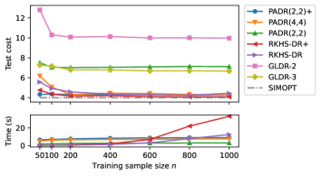
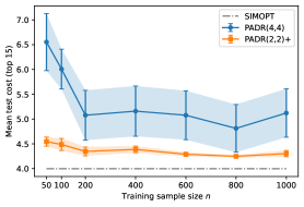
Unconstrained Newsvendor Problem with $\overline{Y}^{\prime}$: Basic Results

b. Varying Feature Dimensions. We set sparse and dense models in the same way as in Section 6.1 and report the comparison results with RKHS-DR and RKHS-DR+ in Figure 1s. PADR(2,2)+ outperforms all the others in both cases. It is worth mentioning that PADR(2,2) is close to PADR(2,2)+ in high-dimensional cases, showing that the training difficulty gradually dominates compared to the value of prior information as the dimension grows. But RKHS-DR+ consistently performs better than RKHS-DR, and it performs better than PADR(2,2) when $p$ is small. As for the running time, PADR(4,4) and PADR(2,2)+ grow linearly with $p$ and are longer than RKHS-DR and RKHS-DR+ only when $p\geq 30$.

(r) Sparse Demand Model               

(s) Dense Demand Model               

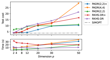
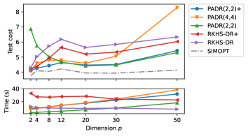
Unconstrained Newsvendor Problem with $\overline{Y}^{\prime}$ and Varying Feature Dimensions

References

- Atamtürk and Hochbaum (2001) Atamtürk A, Hochbaum DS (2001) Capacity acquisition, subcontracting, and lot sizing. Management Science 47(8):1081–1100.
- Balazs et al. (2015) Balazs G, György A, Szepesvari C (2015) Near-optimal max-affine estimators for convex regression. Proceedings of the 18th International Conference on Artificial Intelligence and Statistics (AISTATS), San Diego, CA, 56–64 (PMLR).
- Bampou and Kuhn (2011) Bampou D, Kuhn D (2011) Scenario-free stochastic programming with polynomial decision rules. 50th IEEE Conference on Decision and Control and European Control Conference (CDC-ECC), Orlando, FL, 7806–7812 (IEEE, Piscataway, NJ).
- Ban and Rudin (2018) Ban GY, Rudin C (2018) The big data newsvendor: Practical insights from machine learning. Operations Research 67(1):90–108.
- Bartlett et al. (2002) Bartlett PL, Boucheron S, Lugosi G (2002) Model selection and error estimation. Machine Learning 48(1):85–113.
- Bertsimas and Georghiou (2015) Bertsimas D, Georghiou A (2015) Design of near optimal decision rules in multistage adaptive mixed-integer optimization. Operations Research 63(3):610–627.
- Bertsimas and Kallus (2019) Bertsimas D, Kallus N (2019) From predictive to prescriptive analytics. Management Science 66(3):1025–1044.
- Bertsimas and Koduri (2021) Bertsimas D, Koduri N (2021) Data-driven optimization: A reproducing kernel hilbert space approach. Operations Research 70(1):454–471.
- Beutel and Minner (2012) Beutel AL, Minner S (2012) Safety stock planning under causal demand forecasting. International Journal of Production Economics 140(2):637–645.
- Birge and Louveaux (2011) Birge JR, Louveaux F (2011) Introduction to stochastic programming (Springer Science & Business Media, New York).
- Calafiore and Campi (2005) Calafiore G, Campi MC (2005) Uncertain convex programs: randomized solutions and confidence levels. Mathematical Programming 102(1):25–46.
- Chen et al. (2007) Chen X, Sim M, Sun P, Zhang J (2007) A linear decision-based approximation approach to stochastic programming. Operations Research 56(2):344–357.
- Cui and Pang (2018) Cui Y, Pang JS (2018) On the finite number of directional stationary values of piecewise programs. Preprint, submitted March 1, https://arxiv.org/abs/1803.00190.
- Cui and Pang (2021) Cui Y, Pang JS (2021) Modern Nonconvex Nondifferentiable Optimization (SIAM Publications, Philadelphia).
- Cui et al. (2018) Cui Y, Pang JS, Sen B (2018) Composite difference-max programs for modern statistical estimation problems. SIAM Journal on Optimization 28(4):3344–3374.
- Deng and Gao (2021) Deng Q, Gao W (2021) Minibatch and momentum model-based methods for stochastic weakly convex optimization. 35th Conference Neural Information Processing Systems (NeurIPS 2021), 23115–23127.
- Deng and Sen (2022) Deng Y, Sen S (2022) Predictive stochastic programming. Computational Management Science 19(1):65–98.
- Donti et al. (2017) Donti P, Amos B, Kolter JZ (2017) Task-based end-to-end model learning in stochastic optimization. 31st Conference on Neural Information Processing Systems (NIPS 2017), Long Beach, CA, 5490–5500.
- Drusvyatskiy and Lewis (2018) Drusvyatskiy D, Lewis AS (2018) Error bounds, quadratic growth, and linear convergence of proximal methods. Mathematics of Operations Research 43(3):919–948.
- Elmachtoub and Grigas (2021) Elmachtoub AN, Grigas P (2021) Smart “predict, then optimize”. Management Science 68(1):9–26.
- Ermoliev and Norkin (2013) Ermoliev YM, Norkin VI (2013) Sample average approximation method for compound stochastic optimization problems. SIAM Journal on Optimization 23(4):2231–2263.
- Georghiou et al. (2015) Georghiou A, Wiesemann W, Kuhn D (2015) Generalized decision rule approximations for stochastic programming via liftings. Mathematical Programming 152(1):301–338.
- Hoffman (1952) Hoffman AJ (1952) On approximate solutions of systems of linear inequalities. Journal of Research of the National Bureau of Standards 49(4):263–265.
- Kallus and Mao (2022) Kallus N, Mao X (2022) Stochastic optimization forests. Management Science 0(0).
- Kannan et al. (2022) Kannan R, Bayraksan G, Luedtke JR (2022) Data-driven sample average approximation with covariate information. Preprint, submitted July 27, https://arxiv.org/abs/2207.13554.
- Kao et al. (2009) Kao Yh, Roy B, Yan X (2009) Directed regression. Bengio Y, Schuurmans D, Lafferty J, Williams C, Culotta A, eds., Advances in Neural Information Processing Systems, volume 22, 889–897 (Curran Associates, New York).
- Kuhn et al. (2011) Kuhn D, Wiesemann W, Georghiou A (2011) Primal and dual linear decision rules in stochastic and robust optimization. Mathematical Programming 130(1):177–209.
- Le Thi et al. (2022) Le Thi HA, Huynh VN, Dinh TP, Hau Luu HP (2022) Stochastic difference-of-convex-functions algorithms for nonconvex programming. SIAM Journal on Optimization 32(3):2263–2293.
- Le Thi and Pham Dinh (2018) Le Thi HA, Pham Dinh T (2018) DC programming and DCA: thirty years of developments. Mathematical Programming 169(1):5–68.
- Liu et al. (2022) Liu J, Cui Y, Pang JS (2022) Solving nonsmooth and nonconvex compound stochastic programs with applications to risk measure minimization. Mathematics of Operations Research 47(4):3051–3083.
- Lu et al. (2019) Lu Z, Zhou Z, Sun Z (2019) Enhanced proximal DC algorithms with extrapolation for a class of structured nonsmooth DC minimization. Mathematical Programming 176(1):369–401.
- Luedtke and Ahmed (2008) Luedtke J, Ahmed S (2008) A sample approximation approach for optimization with probabilistic constraints. SIAM Journal on Optimization 19(2):674–699.
- McShane (1934) McShane EJ (1934) Extension of range of functions. Bulletin of the American Mathematical Society 40(12):837–842.
- Mohri et al. (2018) Mohri M, Rostamizadeh A, Talwalkar A (2018) Foundations of machine learning (MIT Press, Cambridge, Massachusetts).
- Nitanda and Suzuki (2017) Nitanda A, Suzuki T (2017) Stochastic difference of convex algorithm and its application to training deep boltzmann machines. Proceedings of the 20th International Conference on Artificial Intelligence and Statistics (AISTATS), Fort Lauderdale, FL, 470–478 (PMLR).
- Notz and Pibernik (2021) Notz PM, Pibernik R (2021) Prescriptive analytics for flexible capacity management. Management Science 68(3):1756–1775.
- Pang et al. (2016) Pang JS, Razaviyayn M, Alvarado A (2016) Computing B-stationary points of nonsmooth DC programs. Mathematics of Operations Research 42(1):95–118.
- Pasupathy and Song (2021) Pasupathy R, Song Y (2021) Adaptive sequential sample average approximation for solving two-stage stochastic linear programs. SIAM Journal on Optimization 31(1):1017–1048.
- Qi et al. (2022) Qi M, Shi Y, Qi Y, Ma C, Yuan R, Wu D, Shen ZJ (2022) A practical end-to-end inventory management model with deep learning. Management Science 69(2):759–773.
- Qi et al. (2021) Qi Z, Cui Y, Liu Y, Pang JS (2021) Asymptotic properties of stationary solutions of coupled nonconvex nonsmooth empirical risk minimization. Mathematics of Operations Research 47(3):2034–2064.
- Scholtes (2012) Scholtes S (2012) Introduction to piecewise differentiable equations (Springer Science & Business Media, New York).
- Shapiro et al. (2021) Shapiro A, Dentcheva D, Ruszczynski A (2021) Lectures on stochastic programming: modeling and theory (SIAM Publications, Philadelphia).
- Siahkamari et al. (2020) Siahkamari A, Gangrade A, Kulis B, Saligrama V (2020) Piecewise linear regression via a difference of convex functions. Proceedings of the 37th International Conference on Machine Learning, 8895–8904 (PMLR).
- Vapnik (1999) Vapnik V (1999) The nature of statistical learning theory (Springer Science & Business Media, New York).
- Xu et al. (2019) Xu Y, Qi Q, Lin Q, Jin R, Yang T (2019) Stochastic optimization for DC functions and non-smooth non-convex regularizers with non-asymptotic convergence. Proceedings of the 36th International Conference on Machine Learning, Long Beach, CA, 6942–6951 (PMLR).