Fingerprinting the Type-Z three Higgs doublet models

Abstract

There has been great interest in a model with three Higgs doublets in which fermions with a particular charge couple to a single and distinct Higgs field. We study the phenomenological differences between the two common incarnations of this so-called Type-Z 3HDM. We point out that the differences between the two models arise from the scalar potential only. Thus we focus on observables that involve the scalar self-couplings. We find it difficult to uncover features that can uniquely set apart the $Z_{3}$ variant of the model. However, by studying the dependence of the trilinear Higgs couplings on the nonstandard masses, we have been able to isolate some of the exclusive indicators for the $Z_{2}\times Z_{2}$ version of the Type-Z 3HDM. This highlights the importance of precision measurements of the trilinear Higgs couplings.

1 Introduction

The Standard Model (SM) of particle physics has been immensely successful in describing the electroweak interaction with great precision. However issues like neutrino mass and dark matter serve as major motivators to look for physics beyond the SM (BSM). Very often, such BSM theories extend the minimal scalar sector of the SM, which consists of only one Higgs-doublet. Therefore, quite naturally, scalar extensions of the SM are routinely investigated in the literature. Among these, multi Higgs-doublet models might be the most ubiquitous, primarily because such extensions preserve the tree-level value of the electroweak $\rho$-parameter. The simplest extension in this category is the two Higgs-doublet model which have been studied extensively[1]. Of late there has been a rise in interest in the study of three Higgs-doublet models (3HDMs)[2, 3] where, as the name suggests, the scalar sector contains three Higgs-doublets.

In the studies of multi Higgs-doublet models it is very often assumed that fermions of a particular charge couple to a single scalar doublet. This will make fermion mass matrices proportional to the corresponding Yukawa matrices and diagonalization of the mass matrices will automatically ensure the simultaneous diagonalization of the Yukawa matrices as well. As a result the model will be free from scalar mediated flavor changing neutral couplings (FCNCs) at the tree-level. In Ref. [4] it was explicitly demonstrated that tree-level FCNCs are absent if and only if there is a basis for the Higgs doublets in which all the fermions of a given electric charge couple to only one Higgs doublet. Such an aspect of the model is quite desirable in view of the flavor data[5]. These types of constructions are usually referred to as models with natural flavor conservation (NFC) [6] in the literature, of which there are five independent possibilities.

Following the terminologies of Ref. [7], one can entertain four types of flavor universal NFC models, namely Type-I, Type-II, Type-X, and Type-Y, within the 2HDM framework. All these Yukawa structures have been concisely summarized in Table 1. Beyond these four options, there is one more interesting possibility where a particular scalar doublet is reserved exclusively for each type of massive fermion. This implies that the up-type quarks, the down-type quarks, and the charged-leptons couple to separate scalar doublets. Evidently, such an arrangement of Yukawa couplings is impossible within a 2HDM framework and one needs at least three scalar doublets to accommodate it. In this paper, we will refer to this possibility as the ‘Type-Z Yukawa’ and subsequently, the 3HDMs that feature a Type-Z Yukawa structure will be collectively called ‘Type-Z 3HDMs’. These Type-Z 3HDMs have gained a lot of attention in the recent past. Theoretical constraints from unitarity and boundedness from below (BFB) have been studied in Refs. [8, 9, 10], the alignment limit is analyzed in Refs. [11, 12], the custodial limit has been studied in Refs. [13], and quite recently, the phenomenological analysis involving the flavor and Higgs data have been performed in Refs. [14, 15]. Other related studies appear in [16, 17, 18, 19].

There are usually two different ways in which a Type-Z Yukawa structure is realized. The first method employs a $Z_{3}$ symmetry[11] whereas the second option uses a $Z_{2}\times Z_{2}$ symmetry[17]. Our objective in this paper will be to point out observable features which can distinguish between the two avatars of Type-Z 3HDMs. Since the Yukawa sector in both versions of Type-Z 3HDM is identical, we will turn our attention to the scalar potential with the hope that some distinguishing aspects can be uncovered. As we will see, only some of the quartic terms in the scalar potential mark the difference between the two variants of Type-Z 3HDM. We will therefore focus on the theoretical constraints from unitarity and BFB which concern the quartic parameters of the scalar potential. We hope that these constraints, in particular, will impact the parameter space in the scalar sector differently for the two Type-Z models. As a result, we expect to encounter some practical distinguishing features of these two models.

Our article will be organized as follows. In Sec. 2 we will outline the two different options for obtaining a Type-Z Yukawa structure along with the corresponding implications for the scalar potential. In Sec. 3 we list the different constraints (both theoretical and phenomenological) faced by the scalar sectors of the 3HDMs under consideration. In Sec. 4 we spell out the details of our numerical analysis and highlight the important outcomes. We summarize our findings and draw our conclusions in Sec. 5.

2 The model

We have already presented the notion of NFC in the introduction. There are a few different ways of obtaining NFC in a 3HDM framework, which have been listed in a concise manner in Table 1 where $\phi_{1}$, $\phi_{2}$ and $\phi_{3}$ represent the three Higgs-doublets that constitute the scalar sector of our model. Among these, we are particularly interested in the possibility of Type-Z Yukawa structure which requires a 3HDM scalar sector at the very least. There are two different ways to ensure a Type-Z Yukawa structure. The first option is to employ a $Z_{3}$ symmetry as follows:

$$\phi_{1}\to e^{2\pi i/3}\,\phi_{1}\,,\qquad\phi_{2}\to e^{4\pi i/3}\phi_{2}\,,\qquad\ell_{R}\to e^{4\pi i/3}\ell_{R}\,,\qquad d_{R}\to e^{2\pi i/3}\,d_{R}\,,$$ (1a)

and the second option will be to use a $$Z_{2}\times Z_{2}^{\prime}$$ symmetry in the following manner:

$$Z_{2}: \phi_{1}\to-\phi_{1}\,,\quad\ell_{R}\to-\ell_{R}\,,$$ (1b)

$$Z^{\prime}_{2}: \phi_{2}\to-\phi_{2}\,,\quad d_{R}\to-d_{R}\,.$$ (1c)

In the equations above the down-type quark and charged-lepton right-handed fields are denoted as $d_{R}$ and $\ell_{R}$, respectively. Since both the symmetries in Eq. (1) entail the same Type-Z Yukawa couplings, we must turn our attention to the scalar sector phenomenologies for possible distinguishable features. The symmetries in Eq. (1) would obviously have their repercussions on the 3HDM scalar potential. To this end we note that the scalar potentials in both these cases consist of a common part as follows:

$$V_{C} = V_{2}+V_{4C}\,,\qquad{\rm where,}$$ (2a)

$$V_{2} = m_{11}^{2}\phi_{1}^{\dagger}\phi_{1}+m_{22}^{2}\phi_{2}^{\dagger}\phi_{2}+m_{33}^{2}\phi_{3}^{\dagger}\phi_{3}-\left[m_{12}^{2}(\phi_{1}^{\dagger}\phi_{2})+m_{13}^{2}(\phi_{1}^{\dagger}\phi_{3})+m_{23}^{2}(\phi_{2}^{\dagger}\phi_{3})+\text{h.c.}\right]\,,$$ (2b)

$$V_{4C} = \lambda_{1}(\phi_{1}^{\dagger}\phi_{1})^{2}+\lambda_{2}(\phi_{2}^{\dagger}\phi_{2})^{2}+\lambda_{3}(\phi_{3}^{\dagger}\phi_{3})^{2}+\lambda_{4}(\phi_{1}^{\dagger}\phi_{1})(\phi_{2}^{\dagger}\phi_{2})+\lambda_{5}(\phi_{1}^{\dagger}\phi_{1})(\phi_{3}^{\dagger}\phi_{3})$$ (2c)

$$+\lambda_{6}(\phi_{2}^{\dagger}\phi_{2})(\phi_{3}^{\dagger}\phi_{3})+\lambda_{7}(\phi_{1}^{\dagger}\phi_{2})(\phi_{2}^{\dagger}\phi_{1})+\lambda_{8}(\phi_{1}^{\dagger}\phi_{3})(\phi_{3}^{\dagger}\phi_{1})+\lambda_{9}(\phi_{2}^{\dagger}\phi_{3})(\phi_{3}^{\dagger}\phi_{2})\,.$$

fermion type	Type-I	Type-II	Type-X	Type-Y	Type-Z
up quarks ($u$)	$\phi_{3}$	$\phi_{3}$	$\phi_{3}$	$\phi_{3}$	$\phi_{3}$
down quarks ($d$)	$\phi_{3}$	$\phi_{2}$	$\phi_{3}$	$\phi_{2}$	$\phi_{2}$
charged leptons ($\ell$)	$\phi_{3}$	$\phi_{2}$	$\phi_{2}$	$\phi_{3}$	$\phi_{1}$

Table 1: Distinct possibilities for NFC in a 3HDM framework. The first four types can also be obtained within 2HDMs but the Type-Z requires at least a 3HDM. In our convention, the scalar doublet coupling to the up-type quarks is always labeled as $\phi_{3}$.

Note that in the expression for $V_{2}$, we have allowed terms that softly break the symmetries defined in Eq. (1). These will be important if we wish to access arbitrarily heavy nonstandard scalars (decoupled from physics at the electroweak scale) without spoiling perturbative unitarity[20, 21, 22]. The differences between the symmetries in Eqs. (1a) and (1b) are captured by the following quartic terms in the scalar potential:

$$V_{Z3} = V_{C}+\left[\lambda_{10}(\phi_{1}^{\dagger}\phi_{2})(\phi_{1}^{\dagger}\phi_{3})+\lambda_{11}(\phi_{1}^{\dagger}\phi_{2})(\phi_{3}^{\dagger}\phi_{2})+\lambda_{12}(\phi_{1}^{\dagger}\phi_{3})(\phi_{2}^{\dagger}\phi_{3})+\text{h.c.}\right]\,,$$ (3a)

$$V_{Z2} = V_{C}+\left[\lambda^{\prime}_{10}(\phi_{1}^{\dagger}\phi_{2})^{2}+\lambda^{\prime}_{11}(\phi_{1}^{\dagger}\phi_{3})^{2}+\lambda^{\prime}_{12}(\phi_{2}^{\dagger}\phi_{3})^{2}+\text{h.c.}\right]\,.$$ (3b)

We, therefore, hope to find distinguishing aspects of these models by tracking the effects of these additional terms.

In order to do this, it is important to conveniently parametrize our models in terms of the physical masses and mixings. We will closely follow the notations and conventions of some earlier works[13, 15]. However, for the sake of completeness, we will give a brief summary of the important expressions which will be crucial for our numerical analysis later. To begin with, let us write the $k$-th scalar doublet, after spontaneous symmetry breaking, as follows:

$$\phi_{k}=\frac{1}{\sqrt{2}}\begin{pmatrix}\sqrt{2}w_{k}^{+}\\ v_{k}+h_{k}+iz_{k}\end{pmatrix}\,,$$ (4)

where $v_{k}$ is the vacuum expectation value (VEV) of $\phi_{k}$, assumed to be real. The three VEVs, $v_{1}$, $v_{2}$ and $v_{3}$ are conveniently parametrized as

$$v_{1}=v\cos\beta_{1}\cos\beta_{2}\,,\quad v_{2}=v\sin\beta_{1}\cos\beta_{2}\,,\quad v_{3}=v\sin\beta_{2}\,,$$ (5)

where $v=\sqrt{v_{1}^{2}+v_{2}^{2}+v_{3}^{2}}$ is the total electroweak (EW) VEV. The component fields in Eq. (4) will mix together and will give rise to two pairs of charged scalars ($H_{1,2}^{\pm}$), two physical pseudoscalars ($A_{1,2}$) and three CP-even neutral scalars ($h,H_{1,2}$). For the charged and pseudoscalar sectors, the physical scalars can be obtained via the following $3\times 3$ rotations,

$$\begin{pmatrix}\omega^{\pm}\\ H_{1}^{\pm}\\ H_{2}^{\pm}\end{pmatrix}=\mathcal{O}_{\gamma_{2}}\mathcal{O}_{\beta}\begin{pmatrix}w_{1}^{\pm}\\ w_{2}^{\pm}\\ w_{3}^{\pm}\end{pmatrix}\;,\quad\quad\begin{pmatrix}\zeta\\ A_{1}\\ A_{2}\end{pmatrix}=\mathcal{O}_{\gamma_{1}}\mathcal{O}_{\beta}\begin{pmatrix}z_{1}\\ z_{2}\\ z_{3}\end{pmatrix},$$ (6)

where, the rotation matrices are given by

$${\cal O}_{\gamma_{1}}=\begin{pmatrix}1&0&0\\ 0&\cos\gamma_{1}&-\sin\gamma_{1}\\ 0&\sin\gamma_{1}&\cos\gamma_{1}\end{pmatrix}\,,\quad{\cal O}_{\gamma_{2}}=\begin{pmatrix}1&0&0\\ 0&\cos\gamma_{2}&-\sin\gamma_{2}\\ 0&\sin\gamma_{2}&\cos\gamma_{2}\end{pmatrix}\,,$$ (7)

and

$${\cal O}_{\beta}=\begin{pmatrix}\cos\beta_{2}\cos\beta_{1}&\cos\beta_{2}\sin\beta_{1}&\sin\beta_{2}\\ -\sin\beta_{1}&\cos\beta_{1}&0\\ -\cos\beta_{1}\sin\beta_{2}&-\sin\beta_{1}\sin\beta_{2}&\cos\beta_{2}\end{pmatrix}.$$ (8)

In Eq. (6), $\omega^{\pm}$ and $\zeta$ stand for the charged and the neutral Goldstone fields respectively. For the CP-even sector, we can obtain the physical scalars as follows:

$$\begin{pmatrix}h\\ H_{1}\\ H_{2}\end{pmatrix} = {\cal O}_{\alpha}\begin{pmatrix}h_{1}\\ h_{2}\\ h_{3}\end{pmatrix}$$ (9)

where

$${\cal O}_{\alpha} = {\cal R}_{3}\cdot{\cal R}_{2}\cdot{\cal R}_{1}\,,$$ (10a)

with

$${\cal R}_{1}=\begin{pmatrix}\cos\alpha_{1}&\sin\alpha_{1}&0\\ -\sin\alpha_{1}&\cos\alpha_{1}&0\\ 0&0&1\end{pmatrix}\,,\quad{\cal R}_{2}=\begin{pmatrix}\cos\alpha_{2}&0&\sin\alpha_{2}\\ 0&1&0\\ -\sin\alpha_{2}&0&\cos\alpha_{2}\end{pmatrix}\,,\quad{\cal R}_{3}=\begin{pmatrix}1&0&0\\ 0&\cos\alpha_{3}&\sin\alpha_{3}\\ 0&-\sin\alpha_{3}&\cos\alpha_{3}\end{pmatrix}.$$ (10b)

Of course, these physical masses and mixings cannot be completely arbitrary as they will have to negotiate a combination of theoretical and phenomenological constraints which will be described in the next section.

3 Constraints

In this section we study the constraints that must be applied to the model parameters in order to ensure theoretical and phenomenological consistency. On the phenomenological side, we first need to guarantee the presence of a SM-like Higgs which will be identified with the scalar boson discovered at the LHC. This can be easily accommodated by staying close to the ‘alignment limit’[11] in 3HDM, defined by the condition

$$\alpha_{1}=\beta_{1}\,,\qquad\alpha_{2}=\beta_{2}\,.$$ (11)

In this limit, the lightest CP-even scalar, $h$, will possess the exact SM-like couplings at the tree-level and constraints from the Higgs signal strengths will be trivially satisfied. However, we will more interested in the extent of deviation from the exact alignment limit allowed from the current measurements of the Higgs signal strengths[23]. We then define the Higgs signal strength as follows:

$$\mu_{i}^{f}=\left(\frac{\sigma_{i}^{\text{3HDM}}(pp\to h)}{\sigma_{i}^{\text{SM}}(pp\to h)}\right)\left(\frac{\text{BR}^{\text{3HDM}}(h\to f)}{\text{BR}^{\text{SM}}(h\to f)}\right)\,,$$ (12)

where the subscript ‘$i$’ denotes the production mode and the superscript ‘$f$’ denotes the decay channel of the SM-like Higgs scalar. Starting from the collision of two protons, the relevant production mechanisms include gluon fusion ($ggF$), vector boson fusion ($VBF$), associated production with a vector boson ($VH$, $V=W$ or $Z$), and associated production with a pair of top quarks ($ttH$). The SM cross section for the gluon fusion process is calculated using HIGLU [24], and for the other production mechanisms we use the prescription of Ref. [25].

Next we need to satisfy the constraints arising from the electroweak $S$, $T$ and $U$ parameters. We will use the analytic expressions derived in Ref. [26] and compare them with the corresponding fit values given in Ref. [27]. It might be worth pointing out that, similar to the 2HDM case, one can easily leap over the $T$-parameter constraints by requiring[13]

$$m_{C1}=m_{A1}\,,\qquad m_{C2}=m_{A2}\,,\qquad\gamma_{1}=\gamma_{2}\,.$$ (13)

We also take into consideration the bounds coming from flavor data. In the Type-Z 3HDM there are no FCNCs at the tree-level. Therefore the only NP contribution at one-loop order to observables such as $b\to s\gamma$ and the neutral meson mass differences will come from the charged scalar Yukawa couplings. It was found in Ref. [14] that the constraints coming from the meson mass differences tend to exclude very low values of $\tan\beta_{1,2}$. Therefore, we only consider

$$\tan\beta_{1,2}>0.3\,,$$ (14)

to safeguard ourselves from the constraints coming from the neutral meson mass differences. To deal with the constraints stemming from $b\to s\gamma$, we follow the procedure described in Refs. [28, 15, 29] and impose the following restriction

$$2.87\times 10^{-4}<\text{BR}(B\to X_{s}\gamma)<3.77\times 10^{-4}\,,$$ (15)

which represents the $3\sigma$ experimental limit.

Additionally, we also take into account the bounds from the direct searches for the heavy nonstandard scalars. For this purpose, we use HiggsBounds-5.9.1 following Ref. [30] where a list of all the relevant experimental searches can be found. It should be noted that we have allowed for decays with off-shell scalar bosons, using the method explained in Ref. [31].

For the theoretical constraints, we first ensure the perturbativity of the Yukawa couplings. For the Type-Z Yukawa structure, the top, bottom, and tau Yukawa couplings are given by

$$y_{t}=\frac{\sqrt{2}\,m_{t}}{v\sin\beta_{2}}\;,\quad y_{b}=\frac{\sqrt{2}\,m_{b}}{v\sin\beta_{1}\cos\beta_{2}}\;,\quad y_{\tau}=\frac{\sqrt{2}\,m_{\tau}}{v\cos\beta_{1}\cos\beta_{2}}\;,$$ (16)

which follow from our convention that $\phi_{3}$, $\phi_{2}$, and $\phi_{1}$ couple to up-type quarks, down-type quarks, and charged leptons respectively. To maintain the perturbativity of Yukawa couplings, we impose $\lvert y_{t}\rvert,\lvert y_{b}\rvert,\lvert y_{\tau}\rvert<\sqrt{4\pi}$. Throughout our paper, we have used values of $\tan\beta_{1,2}$ which are consistent with this perturbative region.

However, we are mainly interested in the effects of the theoretical constraints from perturbative unitarity and BFB conditions. These constraints directly affect the scalar potential and therefore can potentially have different implications for the $Z_{3}$ and $Z_{2}\times Z_{2}$ incarnations of the Type-Z 3HDM. For the unitarity constraints, we use the algorithm presented in Refs. [32, 8]. For the BFB constraints we use only the sufficient conditions of Ref. [15] for the $Z_{3}$ model and the sufficient conditions of Ref. [9] for the $Z_{2}\times Z_{2}$ model.

4 Analysis and results

In both versions of the Type-Z 3HDM the scalar potential of Eq. (2) contains a total of 18 parameters (6 bilinear parameters and 12 quartic parameters). For our numerical analysis, we will trade these 18 parameters in favor of an equivalent but more convenient set of parameters which have a more direct connection to the physical reality. As a first step, we use the minimization conditions to replace three quadratic parameters, $m_{11}^{2}$, $m_{22}^{2}$, and $m_{33}^{2}$, by the three VEVs, $v_{1}$, $v_{2}$, and $v_{3}$ which, in turn, are further exchanged with $v$, $\tan\beta_{1}$, and $\tan\beta_{2}$. The 12 quartic parameters are purposefully interchanged with the 7 physical masses (two charged scalar masses labeled as $m_{C1}$ and $m_{C2}$, two pseudoscalar masses labeled as $m_{A1}$ and $m_{A2}$, and three CP-even scalar masses labeled as $m_{h}$, $m_{H1}$ and $m_{H2}$) and 5 mixing angles appearing in Eqs. (7) and (10).

For each of the symmetry constrained 3HDM, we built a dedicated code, which is an extension of our previous codes [33, 28, 15]. We take $v=246\,\text{GeV}$ and $m_{h}=125\,\text{GeV}$ as experimental inputs. The remaining parameters will be randomly scanned within the following ranges: 

$$\alpha_{1},\,\alpha_{2},\,\alpha_{3},\,\gamma_{1},\,\gamma_{2}\,\in\left[-\frac{\pi}{2},\frac{\pi}{2}\right];\qquad\tan{\beta_{1}},\,\tan{\beta_{2}}\,\in\left[0.3,10\right];$$ (17a)

$$m_{H1}\,,\,m_{H2}\,\in\left[125,1000\right]\,\text{GeV}\,;$$ (17b)

$$m_{A1}\,,\,m_{A2}\,,\,m_{C1}\,,\,m_{C2}\,\in\left[100,1000\right]\,\text{GeV}\,;$$ (17c)

$$m^{2}_{12}\,,m^{2}_{13}\,,m^{2}_{23}\,\in\left[-10^{7},10^{7}\right]\,\text{GeV}^{2}\,.\qquad$$ (17d)

The lower limits chosen for the nonstandard masses satisfy the constraints listed in Ref. [34] and the lower limit on $\tan\beta_{1,2}$ enables us to easily evade the constraints from the meson mass differences.

When studying 3HDM, it was noted [11, 15, 14] that in order to be able to generate good points in an easy way one should not be far away from alignment, defined as the situation where the lightest Higgs scalar has the SM couplings. It was shown in Ref. [11] that this corresponds to the case when

$$\alpha_{1}=\beta_{1}\,,\quad\alpha_{2}=\beta_{2}\,,$$ (18)

with the remaining parameters allowed to be free, although subject to the constraints below. It turns out that for $Z_{3}$ 3HDM [15], this constraint alone is not enough to generate a sufficiently large set of good points starting from a completely unconstrained scan as in Eq. (17d). In Ref. [14] it was noted that all the theoretical and experimental constraints on the scalar sector can be easily negotiated in the ‘maximally symmetric limit’ of 3HDM[35]. As pointed out in Ref. [14] one can easily migrate to the maximally symmetric limit by imposing the following relations among the physical parameters:

$$\gamma_{1}=\gamma_{2}=-\alpha_{3}\,,\quad m_{H1}=m_{A1}=m_{C1}\,,\quad m_{H2}=m_{A2}=m_{C2}\,.$$ (19)

Additionally, the maximally symmetric limit also requires the soft breaking parameters to be related as follows:

$$m^{2}_{12} = c_{\beta_{1}}^{2}c_{\gamma_{2}}s_{\beta_{2}}s_{\gamma_{2}}\left(m_{C1}^{2}-m_{C2}^{2}\right)+c_{\beta_{1}}s_{\beta_{1}}\left[s_{\beta_{2}}^{2}\left(c_{\gamma_{2}}^{2}m_{C2}^{2}+m_{C1}^{2}s_{\gamma_{2}}^{2}\right)-c_{\gamma_{2}}^{2}m_{C1}^{2}-m_{C2}^{2}s_{\gamma_{2}}^{2}\right]$$ (20a)

$$+c_{\gamma_{2}}s_{\beta_{1}}^{2}s_{\beta_{2}}s_{\gamma_{2}}\left(m_{C2}^{2}-m_{C1}^{2}\right)\,,$$

$$m^{2}_{13} = -c_{\beta_{2}}\left[c_{\beta_{1}}s_{\beta_{2}}\left(c_{\gamma_{2}}^{2}m_{C2}^{2}+m_{C1}^{2}s_{\gamma_{2}}^{2}\right)-c_{\gamma_{2}}s_{\beta_{1}}s_{\gamma_{2}}\left(m_{C1}^{2}-m_{C2}^{2}\right)\right]\,,$$ (20b)

$$m^{2}_{23} = -c_{\beta_{2}}\left[c_{\beta_{1}}c_{\gamma_{2}}s_{\gamma_{2}}\left(m_{C1}^{2}-m_{C2}^{2}\right)+s_{\beta_{1}}s_{\beta_{2}}\left(c_{\gamma_{2}}^{2}m_{C2}^{2}+m_{C1}^{2}s_{\gamma_{2}}^{2}\right)\right]\,,$$ (20c)

where $s_{x}$ and $c_{x}$ are shorthands for $\sin x$ and $\cos x$ respectively. Therefore, we can make our numerical study very efficient by strategically scanning in the ‘neighborhood’ of Eqs. (19) and (20).

In a previous phenomenological study of the $Z_{3}$ version of the Type-Z 3HDM [15] we found that one can deviate from the exact relations of Eqs. (18), (19) and (20) by a given percentage (10%, 20%, 50%) thereby enhancing the possibility of new BSM signals, while at the same time being able to generate adequate number of data points. To exemplify, we can ensure to be within $x\%$ of the alignment condition of Eq. (18) by choosing to scan within the following range:

$$\frac{\alpha_{1}}{\beta_{1}}\,,\ \frac{\alpha_{2}}{\beta_{2}}\,\in\,[1-x\%\,,1+x\%]\,.$$ (21)

Extending this prescription we can simultaneously incorporate Eqs. (18) and (19) by scanning within the following range:

$$\frac{\alpha_{1}}{\beta_{1}},\ \frac{\alpha_{2}}{\beta_{2}},\ \frac{\gamma_{2}}{\gamma_{1}},\ \frac{-\alpha_{3}}{\gamma_{1}},\ \frac{m_{A1}}{m_{H1}},\ \frac{m_{C1}}{m_{H1}},\ \frac{m_{A2}}{m_{H2}},\ \frac{m_{C2}}{m_{H2}}\,\in\,[0.8,1.2]\,.\ \ \ \textbf{(Al-20\%)}$$ (22)

The set of points obtained after scanning over the above range will be labeled as ‘Al-20%’ in the subsequent text and plots. In a similar manner we generate another data set labeled as ‘Al-10%’ which are relatively closer to the conditions of Eqs. (18) and (19) by scanning over the following range:

$$\frac{\alpha_{1}}{\beta_{1}},\ \frac{\alpha_{2}}{\beta_{2}},\ \frac{\gamma_{2}}{\gamma_{1}},\ \frac{-\alpha_{3}}{\gamma_{1}},\ \frac{m_{A1}}{m_{H1}},\ \frac{m_{C1}}{m_{H1}},\ \frac{m_{A2}}{m_{H2}},\ \frac{m_{C2}}{m_{H2}}\,\in\,[0.9,1.1]\,.\ \ \ \textbf{(Al-10\%)}$$ (23)

In this context it should be noted that the soft-breaking parameters, whenever they are free, are scanned in a very similar manner in the vicinity of Eq. (20).

$Z_{2}\times Z_{2}$  (AL-10%) Check N Y 100*p 100*$\delta_{p}$ STU 500000 407162 81.432 0.172 BFB 5000000 380066 7.601 0.013 Unitarity 500000 26386 5.277 0.033 $b\rightarrow s\gamma$ 50000 22198 44.396 0.358 $\mu$’s 50000 4168 8.336 0.282 $Z_{3}$  (AL-10%) Check N Y 100*p 100*$\delta_{p}$ STU 500000 407176 81.435 0.172 BFB 5000000 42703 0.854 0.004 Unitarity 500000 18424 3.685 0.027 $b\rightarrow s\gamma$ 50000 21810 43.62 0.354 $\mu$’s 50000 4141 8.282 0.271

Table 2: Impact of individual constraints for the two Type-Z models while the scanning is done following Eq. (23).

To explicitly demonstrate the efficiency of our scanning method, we display in Table 2 how restrictive the individual constraints of Sec. 3 can be. In these tables, $N$ represents the number of initial input points and $Y$ stands for the number of output points that can successfully pass through a given constraint labeled appropriately. Thus $p=Y/N$ gives an estimate for the probability of successfully negotiating a particular constraint. The quantity $\delta_{p}$ represents the typical uncertainty associated with the estimate of $p$ and is calculated using the formula for the propagation of errors. From Table 2 it should be evident that the BFB constraints have a very low acceptance ratio for the input points. We should point out that our choice of scanning around Eqs. (18) and (19) does definitely increase the number of output points that pass through all the constraints. This is detailed in the Appendix, where we show equivalent numbers for a run generating points within 50% of the alignment limit.

Now that our scan strategy has been laid-out clearly, we can proceed to describe the results from our numerical studies. We will do this in two stages. At first we will demonstrate the results from the general scans and point out features that may distinguish between the two variants of Type-Z 3HDMs. In the second part we will presume that some nonstandard scalars have been discovered and therefore we will work with some illustrative benchmark points in the hope of making the distinction between the two models more pronounced.

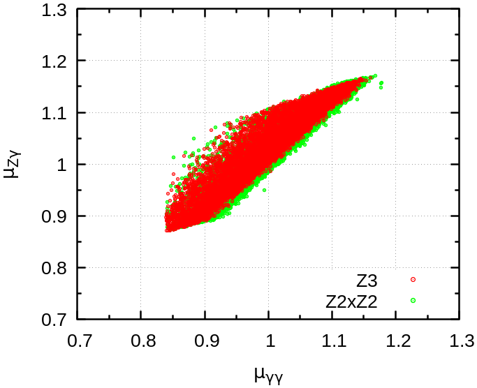
Figure 1: Output points that pass all the constraints are plotted in $\mu_{\gamma\gamma}$ vs $\mu_{Z\gamma}$ plane for the gluon fusion production channel. The scanning is done assuming the Al-10% condition of Eq. (23). The red and the green points correspond to the $Z_{3}$ and $Z_{2}\times Z_{2}$ models respectively.

We have to always keep in mind that the difference between the two versions of Type-Z 3HDM is marked by the scalar potential. Therefore, we focus on the measurements that involve the scalar self-couplings. Quite naturally, our first choice will be to study $\mu_{\gamma\gamma}$ and $\mu_{Z\gamma}$ (Higgs signal strengths in the two photon and $Z$-photon channels respectively) which pick up extra contributions from charged scalar loops that depend on couplings of the form $hH_{i}^{+}H_{i}^{-}$ ($i=1,2$). However, as we have displayed in Fig. 1, the points that pass through all the constraints span very similar regions in the $\mu_{\gamma\gamma}$ vs $\mu_{Z\gamma}$ plane for both versions of Type-Z 3HDM. Thus no significant distinction between the two models can be made from $\mu_{\gamma\gamma}$ and $\mu_{Z\gamma}$.

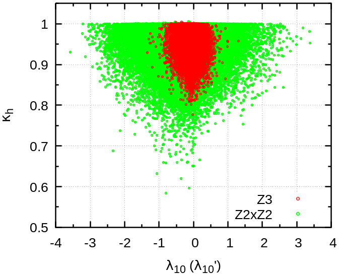
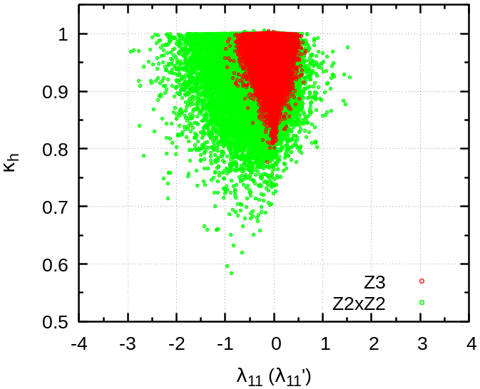
Figure 2: Points that pass through all the constraints are plotted in the $\kappa_{h}$ vs $\lambda_{10}^{(\prime)},\lambda_{11}^{(\prime)},\lambda_{12}^{(\prime)}$ plane. The scanning is done assuming the Al-10% condition of Eq. (23). The red and the green points correspond to the $Z_{3}$ and $Z_{2}\times Z_{2}$ models respectively.

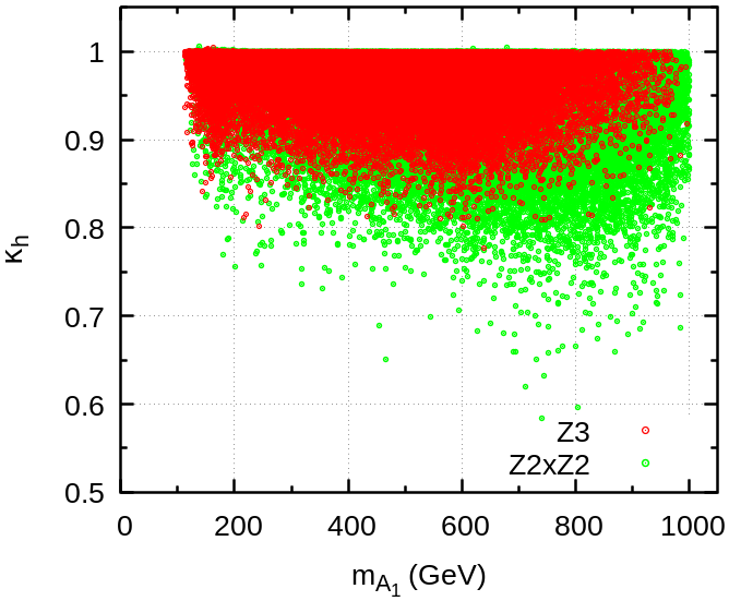
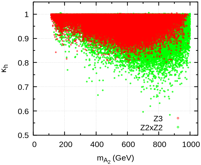
Figure 3: Points that pass through all the constraints are plotted in the $\kappa_{h}$ vs $m_{A1},m_{A2}$ plane. The scanning is done assuming the Al-10% condition of Eq. (23). The red and the green points correspond to the $Z_{3}$ and $Z_{2}\times Z_{2}$ models respectively.

Next we turn our attention to the trilinear Higgs self-coupling of the following form:

$${\mathscr{L}}_{hhh}=g_{hhh}h^{3}\,.$$ (24)

In the SM we have $g_{hhh}^{\rm SM}=-m_{h}^{2}/(2v)$. Thus we define the following coupling modifier

$$\kappa_{h}=\frac{g_{hhh}}{g_{hhh}^{\rm SM}}$$ (25)

which is already being measured experimentally and some preliminary values have been reported in Refs. [36, 37]. We have checked that for both the Type-Z models, $\kappa_{h}=1$ in the alignment limit defined by Eq. (18), as expected. Therefore we have to hope that the LHC Higgs data will eventually settle for some nonstandard values away from exact alignment so that some distinguishing features can be found. To this end we recall that the quartic parameters of Eq. (3) mark the essential difference between the two models. It should also be noted that in the limit $\lambda_{10}^{(\prime)},\lambda_{11}^{(\prime)},\lambda_{12}^{(\prime)}=0$, the quartic part of the potential possesses a $U(1)\times U(1)$ symmetry (independent from the $U(1)_{Y}$ hypercharge symmetry). Consequently, $\lambda_{10}^{(\prime)}$, $\lambda_{11}^{(\prime)}$ and $\lambda_{12}^{(\prime)}$ are the only quartic parameters that get involved in the expressions of the pseudoscalar masses, $m_{A1}$ and $m_{A2}$. Keeping these in mind we exhibit in Fig. 2 the scatter plot of the points that pass through all the constraints in the $\kappa_{h}$ vs $\lambda_{10}^{(\prime)},\lambda_{11}^{(\prime)},\lambda_{12}^{(\prime)}$ plane. There we observe that values of $\kappa_{h}$ in the ballpark $0.8$ or lower will definitely favor the $Z_{2}\times Z_{2}$ scenario over the $Z_{3}$ version of Type-Z 3HDM. To give these results a better physical context, in Fig. 3, we plot the same points in the $\kappa_{h}$ vs pseudoscalar mass planes. This figure clearly indicates that unlike the $Z_{3}$ model, the $Z_{2}\times Z_{2}$ model can still allow $\kappa_{h}$ values as low as $0.7$. In passing, we also note that values of $\kappa_{h}$ around $1.1$ or higher will disfavor both versions of Type-Z 3HDMs.

	$m_{H1}$	$m_{H2}$	$m_{A1}$	$m_{A2}$	$m_{C1}$	$m_{C2}$
Benchmark 1	365	450	340	470	335	465
Benchmark 2	530	645	515	610	540	610
Benchmark 3	641	775	615	745	645	770

Table 3: Benchmark values for the nonstandard masses (in GeV) used in Fig. 4.

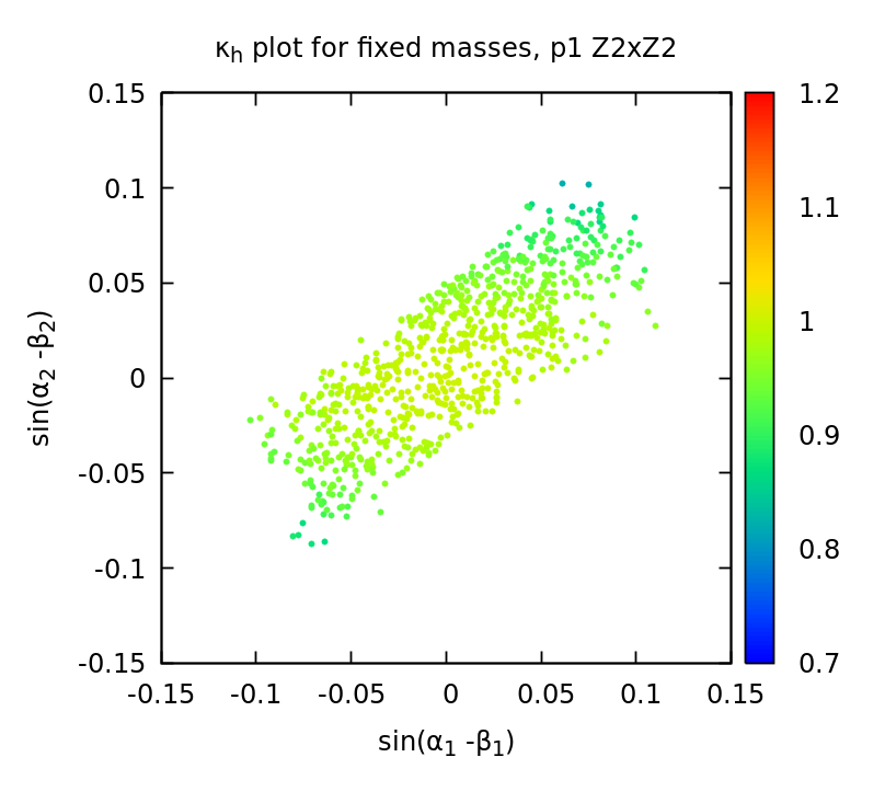
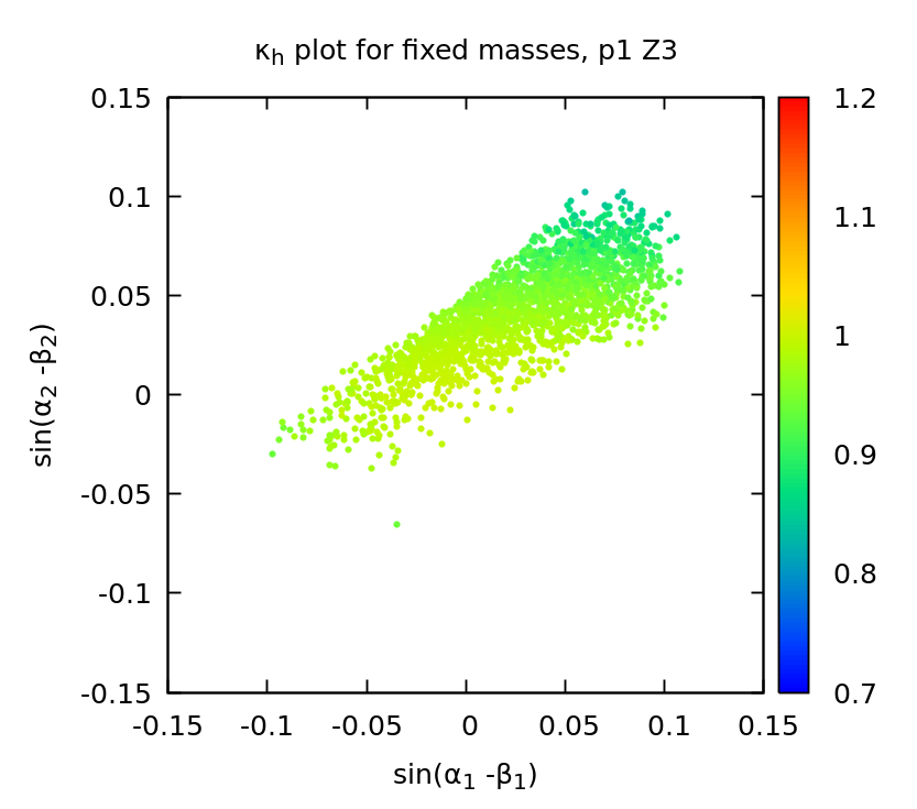
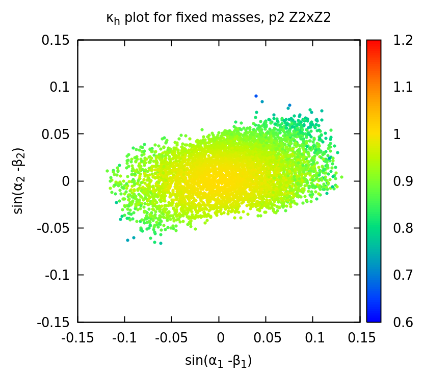
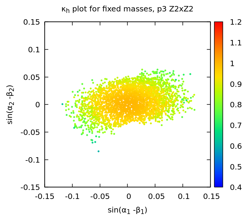
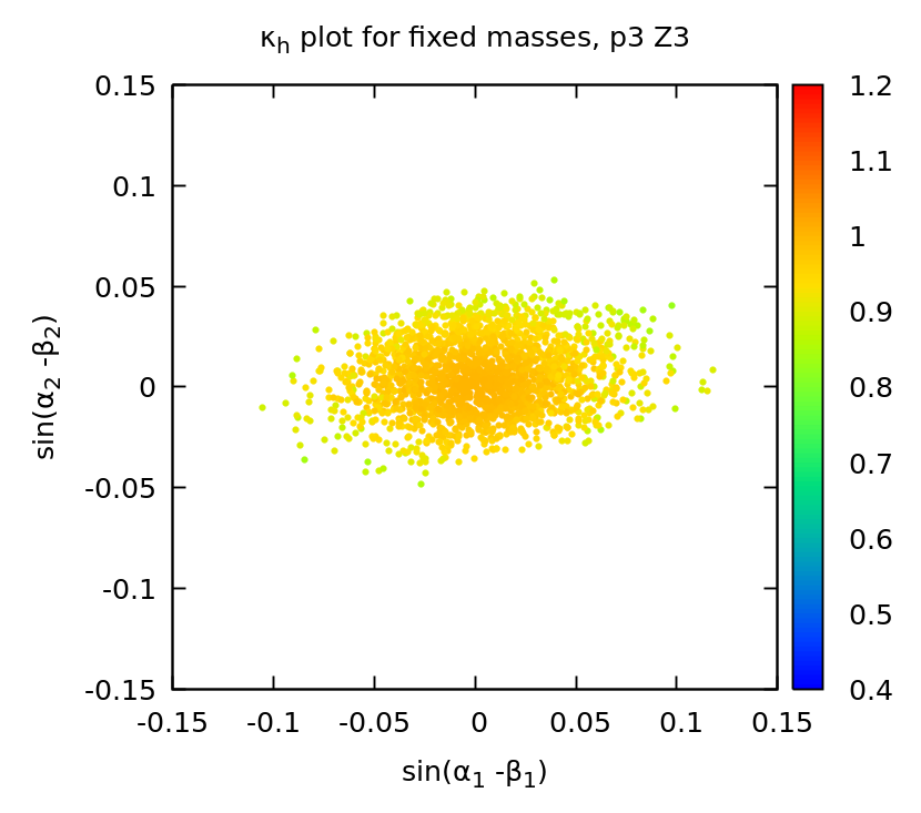
Figure 4: Plot in the $\sin{(\alpha_{1}-\beta_{1})}$ vs $\sin{(\alpha_{1}-\beta_{1})}$ plane for the benchmark values (labeled appropriately) of Table 3. The color bar associated with each plot marks the gradient of values taken by $\kappa_{h}$. The plots in the left panel correspond to the $Z_{2}\times Z_{2}$ model whereas the plots in the right panel correspond to the $Z_{3}$ model. Clearly, the distinguishability between the two models depends on the benchmark point (mass region) chosen.

In a final and more optimistic effort, we presume that some nonstandard scalars have already been observed and we try to ascertain whether, in view of the set of nonstandard parameters, one of the Type-Z 3HDMs can be preferred over the other. Our benchmark values for the nonstandard masses appear in Table 3. The remaining parameters are scanned following Eq. (22). For these benchmark values we have plotted all the points that pass through the constraints in the $\sin(\alpha_{1}-\beta_{1})$ vs $\sin(\alpha_{2}-\beta_{2})$ plane. The results have been displayed in Fig. 4 where we have also color coded the value of $\kappa_{h}$ for each point. There we can see that the points span a relatively larger region for the $Z_{2}\times Z_{2}$ model. Therefore, if both $\sin(\alpha_{1}-\beta_{1})$ and $\sin(\alpha_{2}-\beta_{2})$ are measured to be close to $0.1$ along with $\kappa_{h}$ to be around $0.7$, then it would definitely point towards the $Z_{2}\times Z_{2}$ model. Thus, again, we have found that although we can find corners in the parameter space that can isolate the $Z_{2}\times Z_{2}$ model, it seems to be very difficult to point out exclusive features characterizing the $Z_{3}$ version of the Type-Z 3HDM.

5 Summary

To summarize, we have studied the two common incarnations of Type-Z 3HDMs. One of them employs a $Z_{2}\times Z_{2}$ symmetry while the other relies on a $Z_{3}$ symmetry. We point out that the difference between these two models is captured by certain quartic terms in the scalar potential appearing in Eq. (3). Then we proceed to uncover the effects of these quartic terms in creating distinctions between the two Type-Z models.

In doing so we have performed exhaustive scans over the set of free parameters in these models. Wherever possible, we have conveniently traded the Lagrangian parameters in favor of the physical masses and mixings. Even then, when all the relevant theoretical and experimental constraints are imposed, a completely random scan generates very few output points that successfully negotiate all the constraints. Therefore, we adopt a more strategic scanning procedure which involve generating random points around a premeditated proximity of the ‘maximally symmetric limit’ defined by Eq. (19). In this way we have successfully generated sufficient number of points to populate our plots.

For the plots, we were mainly interested in observables that involve the Higgs self couplings. We have found that although $\mu_{\gamma\gamma}$ and $\mu_{Z\gamma}$ are not the best discriminators, the trilinear Higgs self coupling modifier $(\kappa_{h})$ has the potential to distinguish between the two models. We have concluded that relatively lower values of $\kappa_{h}$ will favor the $Z_{2}\times Z_{2}$ version of Type-Z 3HDM. We have also emphasized that some nonstandard physics need to be discovered in the LHC Higgs data for us to be able to discriminate between the two Type-Z 3HDMs. Our study underscores the importance of the ongoing effort to measure the trilinear Higgs self coupling with increased precision.

Appendix A Impact of a wider search

In order to assess the need for a search of points close to the alignment limit of Eqs. (18) and (19), we redo Table 2, now with the looser bounds

$$\frac{\alpha_{1}}{\beta_{1}},\ \frac{\alpha_{2}}{\beta_{2}},\ \frac{\gamma_{2}}{\gamma_{1}},\ \frac{-\alpha_{3}}{\gamma_{1}},\ \frac{m_{A1}}{m_{H1}},\ \frac{m_{C1}}{m_{H1}},\ \frac{m_{A2}}{m_{H2}},\ \frac{m_{C2}}{m_{H2}}\,\in\,[0.5,1.5]\,.\ \ \ \textbf{(Al-50\%)}$$ (26)

$Z_{2}\times Z_{2}$ (Al-50%) Check N Y 100*p 100*$\delta_{p}$ STU 500000 46179 9.236 0.045 BFB 5000000 277802 5.556 0.011 Unitarity 500000 3397 0.679 0.012 $b\rightarrow s\gamma$ 50000 19340 38.680 0.328 $\mu$’s 50000 217 0.434 0.077 $Z_{3}$  (Al-50%) Check N Y 100*p 100*$\delta_{p}$ STU 500000 46296 9.259 0.045 BFB 5000000 25673 0.513 0.003 Unitarity 500000 2639 0.528 0.010 $b\rightarrow s\gamma$ 50000 19193 38.386 0.326 $\mu$’s 50000 178 0.356 0.069

Table 4: Impact of individual constraints for the two Type-Z models while the scanning is done following Eq. (26).

Comparing Table 2 with Table 4, we notice that, away from alignment, the unitarity and $\mu$ constraints cut most of the allowed parameter space.

References

- [1] G. C. Branco, P. M. Ferreira, L. Lavoura, M. N. Rebelo, M. Sher, and J. P. Silva, Theory and phenomenology of two-Higgs-doublet models, Phys. Rept. 516 (2012) 1–102, [arXiv:1106.0034].
- [2] V. Keus, S. F. King, and S. Moretti, Three-Higgs-doublet models: symmetries, potentials and Higgs boson masses, JHEP 01 (2014) 052, [arXiv:1310.8253].
- [3] I. P. Ivanov and E. Vdovin, Classification of finite reparametrization symmetry groups in the three-Higgs-doublet model, Eur. Phys. J. C 73 (2013), no. 2 2309, [arXiv:1210.6553].
- [4] P. M. Ferreira, L. Lavoura, and J. P. Silva, Renormalization-group constraints on Yukawa alignment in multi-Higgs-doublet models, Phys. Lett. B 688 (2010) 341–344, [arXiv:1001.2561].
- [5] Particle Data Group Collaboration, R. L. Workman et al., Review of Particle Physics, PTEP 2022 (2022) 083C01.
- [6] S. L. Glashow and S. Weinberg, Natural Conservation Laws for Neutral Currents, Phys. Rev. D 15 (1977) 1958.
- [7] K. Yagyu, Higgs boson couplings in multi-doublet models with natural flavour conservation, Phys. Lett. B 763 (2016) 102–107, [arXiv:1609.04590].
- [8] M. P. Bento, J. C. Romão, and J. P. Silva, Unitarity bounds for all symmetry-constrained 3HDMs, JHEP 08 (2022) 273, [arXiv:2204.13130].
- [9] R. Boto, J. C. Romão, and J. P. Silva, Bounded from below conditions on a class of symmetry constrained 3HDM, Phys. Rev. D 106 (2022), no. 11 115010, [arXiv:2208.01068].
- [10] S. Moretti and K. Yagyu, Constraints on Parameter Space from Perturbative Unitarity in Models with Three Scalar Doublets, Phys. Rev. D 91 (2015) 055022, [arXiv:1501.06544].
- [11] D. Das and I. Saha, Alignment limit in three Higgs-doublet models, Phys. Rev. D 100 (2019), no. 3 035021, [arXiv:1904.03970].
- [12] A. Pilaftsis, Symmetries for standard model alignment in multi-Higgs doublet models, Phys. Rev. D 93 (2016), no. 7 075012, [arXiv:1602.02017].
- [13] D. Das, M. Levy, P. B. Pal, A. M. Prasad, I. Saha, and A. Srivastava, Democratic three Higgs-doublet models: the custodial limit and wrong-sign Yukawa, arXiv:2301.00231.
- [14] M. Chakraborti, D. Das, M. Levy, S. Mukherjee, and I. Saha, Prospects for light charged scalars in a three-Higgs-doublet model with Z3 symmetry, Phys. Rev. D 104 (2021), no. 7 075033, [arXiv:2104.08146].
- [15] R. Boto, J. C. Romão, and J. P. Silva, Current bounds on the type-Z Z3 three-Higgs-doublet model, Phys. Rev. D 104 (2021), no. 9 095006, [arXiv:2106.11977].
- [16] G. Cree and H. E. Logan, Yukawa alignment from natural flavor conservation, Phys. Rev. D 84 (2011) 055021, [arXiv:1106.4039].
- [17] A. G. Akeroyd, S. Moretti, K. Yagyu, and E. Yildirim, Light charged Higgs boson scenario in 3-Higgs doublet models, Int. J. Mod. Phys. A 32 (2017), no. 23n24 1750145, [arXiv:1605.05881].
- [18] J. M. Alves, F. J. Botella, G. C. Branco, and M. Nebot, Extending trinity to the scalar sector through discrete flavoured symmetries, Eur. Phys. J. C 80 (2020), no. 8 710, [arXiv:2005.13518].
- [19] H. E. Logan, S. Moretti, D. Rojas-Ciofalo, and M. Song, CP violation from charged Higgs bosons in the three Higgs doublet model, JHEP 07 (2021) 158, [arXiv:2012.08846].
- [20] G. Bhattacharyya and D. Das, Nondecoupling of charged scalars in Higgs decay to two photons and symmetries of the scalar potential, Phys. Rev. D 91 (2015) 015005, [arXiv:1408.6133].
- [21] S. Carrolo, J. C. Romão, J. P. Silva, and F. Vazão, Symmetry and decoupling in multi-Higgs boson models, Phys. Rev. D 103 (2021), no. 7 075026, [arXiv:2102.11303].
- [22] F. Faro, J. C. Romão, and J. P. Silva, Nondecoupling in Multi-Higgs doublet models, Eur. Phys. J. C 80 (2020), no. 7 635, [arXiv:2002.10518].
- [23] ATLAS Collaboration, A detailed map of Higgs boson interactions by the ATLAS experiment ten years after the discovery, Nature 607 (2022), no. 7917 52–59, [arXiv:2207.00092]. [Erratum: Nature 612, E24 (2022)].
- [24] M. Spira, HIGLU: A program for the calculation of the total Higgs production cross-section at hadron colliders via gluon fusion including QCD corrections, hep-ph/9510347.
- [25] LHC Higgs Cross Section Working Group Collaboration, D. de Florian et al., Handbook of LHC Higgs Cross Sections: 4. Deciphering the Nature of the Higgs Sector, arXiv:1610.07922.
- [26] W. Grimus, L. Lavoura, O. M. Ogreid, and P. Osland, A Precision constraint on multi-Higgs-doublet models, J. Phys. G 35 (2008) 075001, [arXiv:0711.4022].
- [27] Gfitter Group Collaboration, M. Baak, J. Cúth, J. Haller, A. Hoecker, R. Kogler, K. Mönig, M. Schott, and J. Stelzer, The global electroweak fit at NNLO and prospects for the LHC and ILC, Eur. Phys. J. C 74 (2014) 3046, [arXiv:1407.3792].
- [28] R. R. Florentino, J. C. Romão, and J. P. Silva, Off diagonal charged scalar couplings with the Z boson: Zee-type models as an example, Eur. Phys. J. C 81 (2021), no. 12 1148, [arXiv:2106.08332].
- [29] A. G. Akeroyd, S. Moretti, T. Shindou, and M. Song, CP asymmetries of in models with three Higgs doublets, Phys. Rev. D 103 (2021), no. 1 015035, [arXiv:2009.05779].
- [30] P. Bechtle, D. Dercks, S. Heinemeyer, T. Klingl, T. Stefaniak, G. Weiglein, and J. Wittbrodt, HiggsBounds-5: Testing Higgs Sectors in the LHC 13 TeV Era, Eur. Phys. J. C 80 (2020), no. 12 1211, [arXiv:2006.06007].
- [31] J. C. Romão and S. Andringa, Vector boson decays of the Higgs boson, Eur. Phys. J. C 7 (1999) 631–642, [hep-ph/9807536].
- [32] M. P. Bento, H. E. Haber, J. C. Romão, and J. P. Silva, Multi-Higgs doublet models: physical parametrization, sum rules and unitarity bounds, JHEP 11 (2017) 095, [arXiv:1708.09408].
- [33] D. Fontes, J. C. Romão, and J. P. Silva, in the complex two Higgs doublet model, JHEP 12 (2014) 043, [arXiv:1408.2534].
- [34] A. Aranda, D. Hernández-Otero, J. Hernández-Sanchez, V. Keus, S. Moretti, D. Rojas-Ciofalo, and T. Shindou, Z3 symmetric inert ( 2+1 )-Higgs-doublet model, Phys. Rev. D 103 (2021), no. 1 015023, [arXiv:1907.12470].
- [35] N. Darvishi, M. R. Masouminia, and A. Pilaftsis, Maximally symmetric three-Higgs-doublet model, Phys. Rev. D 104 (2021), no. 11 115017, [arXiv:2106.03159].
- [36] CMS Collaboration, A. Tumasyan et al., Search for Higgs Boson Pair Production in the Four b Quark Final State in Proton-Proton Collisions at s=13 TeV, Phys. Rev. Lett. 129 (2022), no. 8 081802, [arXiv:2202.09617].
- [37] ATLAS Collaboration, G. Aad et al., Search for Higgs boson pair production in the two bottom quarks plus two photons final state in collisions at TeV with the ATLAS detector, Phys. Rev. D 106 (2022), no. 5 052001, [arXiv:2112.11876].