Energy-Efficient Precoding and Feeder-Link-Beam Matching Design for Bent-Pipe SATCOM Systems

Abstract

This paper proposes a joint optimization framework for energy-efficient precoding and feeder-link-beam matching design in a multi-gateway multi-beam bent-pipe satellite communication system. The proposed scheme jointly optimizes the precoding vectors at the gateways and amplifying-and-matching mechanism at the satellite to maximize the system weighted energy efficiency under the transmit power budget constraint. The technical designs are formulated into a non-convex sparsity problem consisting of a fractional-form objective function and sparsity-related constraints. To address these challenges, two iterative efficient designs are proposed by utilizing the concepts of Dinkelbach’s method and the compress-sensing approach. The simulation results demonstrate the effectiveness of the proposed scheme compared to another benchmark method.

I Introduction

Recently, satellite communication (SATCOM) have been considered as an important component of the next generation of wireless communication which can enable seamless global connectivity. To meet the increasing high-data-rate demand, advanced satellite communication technologies have been developed for the traditional bent-pipe payload, including multi-gateway and multi-beam transmission [1]. Multiple gateways (GWs) deployed in various areas can provide flexible and resilient connections between the ground segments and satellites [1] while precoding-enabled multi-beam transmission can mitigate the interference and improve the network performance significantly [2, 3]. Regarding both user and feeder links (FLs) in precoding design, this advanced SATCOM system poses significant energy-efficient challenges, including the matching and amplifying strategies at payload.

In recent years, several works have been proposed to optimize the energy efficiency of multi-beam SATCOM systems. In [4], Chatzinotas et al. focused on investigating the energy efficiency of a multi-beam downlink system using Minimum Mean Square Error (MMSE) beamforming and power optimization for the satellite downlink channel. In [5], Qi et al. considered the design of energy-efficient multicast precoding for multi-user multi-beam SATCOMs under total power and Quality of Service (QoS) constraints. In [6], Abdu et al. proposed an energy-efficient sparse precoding design for SATCOM systems, where only a few precoding coefficients are used with lower transmit power consumption depending on demand. Additionally, Joroughi et al. in [7] analyze the precoding scheme in a multi-GW multi-beam satellite system. The studied design is developed by utilizing a regularized singular value block decomposition of the channel matrix to minimize both inter-cluster and intra-cluster interference. These studies demonstrate the importance of energy-efficient and multi-beam precoding designs in SATCOMs; however, they have not considered the impact of the FLs in their optimization frameworks.

This paper considers an end-to-end forward link of a broadband multi-GW multi-beam bent-pipe SATCOM system serving a number of ground users. In this scheme, the user signals are precoded at the GWs, before being transmitted to the satellite through MIMO-enabled FLs. Then, these signals are amplified, and matched to beams for forwarding to the end users. The system poses significant challenges for energy-efficient design due to the precoding tasks, matching and amplifying mechanisms, and limited transmission-power budgets. To address these challenges, we propose a joint optimization framework for energy-efficient precoding, FL-beam matching, and amplify design. The proposed scheme optimizes the precoding vectors at the GWs and sparsity variables regarding the forwarding process at the satellite to maximize the system’s energy efficiency under the transmit power budget constraints. Dinkelbach’s method and compress-sensing approach are then employed to address the fractional-form objective function and sparsity-related critical issues. The work provides two energy-efficient solutions balancing the overall power consumption and the Quality of Service (QoS) for all users. The simulation results are also presented to highlight the superior performance of the proposed approaches in comparison to another benchmark technique.

II System Model and Problem Formulation

II-A End-to-end Multi-GW Multi-beam SATCOM Systems

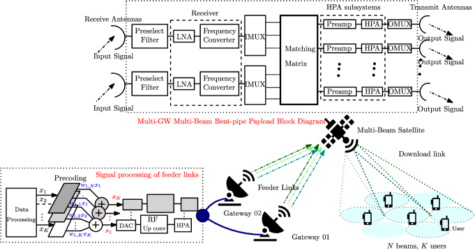
Figure 1: Structure and transmission diagram of a multi-GW multi-beam bent-pipe SATCOM system.

Consider an end-to-end forward link of a broadband multi-beam bent-pipe satellite system consisting of multiple GWs with $L$ antennas on the ground, a bent-pipe transparent satellite (GEO, MEO, or LEO) equipped with $L$ receiving and $N$ transmission elements, and $K$ remote single-antenna users. In this system, the precoding vectors are applied to the corresponding symbol sequences for users at the GW. These precoded signals are sent to the satellite through the MIMO-enabled FLs. The received signals are then amplified and forwarded to the end users by the satellite payload.

II-A1 MIMO-enabled Feeder Links

In this work, an $L\times L$ MIMO transmission assumed for the communication between GWs and satellite with full re-use frequency of Q/V-band ($42.5-43.5$ GHz and $47.2-50.2$ GHz) [8]. At these higher frequencies, links to the satellite indeed use highly directional antennas such that strong LOS connections are established. Let $S$ be the number of sub-carrier channelized in FLs. Hence, the FLs can support at most $SL$ streams at a specific time. Here, we assume $N=SL$. Following [8], the FL channel matrix, i.e., $\mathbf{F}$, can be modelled as

$$\mathbf{F}=\text{diag}\{\mathbf{F}_{(1)},\mathbf{F}_{(2)},...,\mathbf{F}_{(S)}\}.$$ (1)

In this equation, $\mathbf{F}_{(s)}\in\mathbb{C}^{L\times L}$ represents the FL channel matrix of sub-carrier $s$ which can be expressed as

$$\mathbf{F}_{(s)}=\scaleobj{.8}{\sqrt{G_{(s)}^{\sf{GW}}G_{(s)}^{\sf{Sa-Rx}}}}\tilde{\mathbf{F}}_{(s)}\boldsymbol{\alpha}_{(s)},$$ (2)

where $G_{(s)}^{\sf{GW}},G_{(s)}^{\sf{Sa-Rx}}$ are the antenna gains at GW and satellite, $\tilde{\mathbf{F}}_{(s)}\in\mathbb{C}^{L\times L}$ models the LOS free-space propagation. Here, the $(m,n)$-entry of $\tilde{\mathbf{F}}_{(s)}$ is given by $[\tilde{F}^{(s)}]_{(m,n)}=\exp\{-j(\psi_{m,n}+\phi_{m,n})\}/\psi_{m,n}$ where $\psi_{m,n}={4\pi f_{(s)}^{c}r_{m,n}}/{c_{0}}$ and $\phi_{m,n}$ represents the miss-synchronization phase noise. In addition, $\boldsymbol{\alpha}_{(s)}\in\mathbb{C}^{L\times L}$ is a diagonal matrix of the atmospheric impairments experienced at the GWs [8]. The $l$-th diagonal element of $\boldsymbol{\alpha}_{(s)}$ can be given as $\alpha^{(s)}_{l}=|\alpha_{l}|\exp\{-j\xi^{(s)}_{l}\}$ where $|\alpha_{l}|\in(0,1]$ and $\xi^{(s)}_{l}\in[-\pi,\pi]$ represents the amplitude fading and phase shift, respectively.

II-A2 User Links

Let $\mathbf{H}\in\mathbb{C}^{N\times K}$ be the channel matrix of the satellite-user links. Herein, $[\mathbf{H}]_{(n,u)}=h_{n,u}$ stands for the channel coefficient from antenna $n$ to user $u$ which can be modeled using Rician channel model [3] as,

$$h_{n,u}\!=\!\scaleobj{.7}{\dfrac{\sqrt{G^{\sf{gu}}_{u}}}{\psi_{u}}}e^{-j\left(\psi_{u}+\phi_{n,u}\right)}\left(\scaleobj{.7}{\sqrt{\dfrac{\kappa}{\kappa+1}}}p^{\sf{pa}}_{n,u}+\scaleobj{.7}{\sqrt{\dfrac{1}{\kappa+1}}}\alpha_{n,u}\right),$$ (3)

where $G^{\sf{gu}}_{u}$ is the antenna receiving gain of user $u$; $\psi_{u}=\frac{2\pi d_{u}}{\lambda}$, $d_{u}$ is the distance between the satellite and user $u$, $p^{\sf{pa}}_{n,u}$ represents the pattern coefficient of beam $n$ which includes the amplitude and phase corresponding to the user’s location; $\alpha_{n,u}$ is the small NLoS fading; $\kappa$ denotes Rician factor; $\lambda$ is the wave length, and $\phi^{n,u}$ stands for the phase noise.

II-A3 Gateway Linear Precoding

Due to $N$ transmission elements, one assumes the satellite can generate at most $N$ satellite beams for user-link transmission. Let $\mathbf{w}_{u}=[w_{1,u},w_{2,u},...,w_{N,u}]^{T}\in\mathbb{C}^{N\times 1}$ be the DP vector designed for symbol sequence of user $u$, named $x_{u}\in\mathbb{C}$ and $\mathbb{E}_{x_{u}}\{|x_{u}|\}=1$. Considering the signal processing design, the GWs first apply all DP vector $\mathbf{w}_{u}$’s to the symbol sequences of all users. The precoded signals can be written as

$$\mathbf{s}=\scaleobj{.8}{\sum_{u\in\mathcal{U}}}\mathbf{w}_{u}x_{u},$$ (4)

where $\mathbf{s}\in\mathbb{C}^{N\times 1}$ and $\mathcal{U}$ stands for the set of users. Then, $\mathbf{s}$ will be sent to the satellite over FLs with channel-matrix $\mathbf{F}$. The received signal at the satellite can be expressed as

$$\mathbf{r}=\mathbf{F}^{H}\mathbf{s}+\mathbf{n}^{\mathrm{fd}}=\mathbf{F}^{H}\scaleobj{.8}{\sum_{u\in\mathcal{U}}}\mathbf{w}_{u}x_{u}+\mathbf{n}^{\mathrm{fd}},$$ (5)

where $\mathbf{n}^{\mathrm{fd}}\in\mathbb{C}^{N\times 1}$ is an AWGN vector at the satellite.

II-A4 Payload Matching and Amplying Process

At the satellite, $N$ signal streams corresponding to $N$ FLs, i.e $\mathbf{r}$, are amplified and then matched to $N$ beams for propagation to users over the user links. Let $\mathbf{B}\in\mathbb{R}_{+}^{N\times N}$ be the amplifying and matching matrix between $N$ signal streams of $\mathbf{r}$ to $N$ beams. Denote $[\mathbf{B}]_{n,t}=b_{n,t}$ as an element locating on the $t$-th row and $n$-th column of $\mathbf{B}$, we have

$$\left\{\begin{array}[]{*{10}{l}}b_{n,t}>0,&\text{if $[\mathbf{r}]_{t}$ is transmitted over beam $n$,}\\ b_{n,t}=0,&\text{otherwise}.\end{array}\right.$$ (6)

Due to the matching policy, $\mathbf{B}$ must be designed by regarding the following constraints,

$$(C1):\scaleobj{.8}{\sum_{\forall t}}\|b_{n,t}\|_{0}\leq 1,\forall n,\text{ and }(C2):\scaleobj{.8}{\sum_{\forall n}}\|b_{n,t}\|_{0}\leq 1,\forall t,$$ (7)

where $\|x\|_{0}$ stands for the norm-$0$ of $x$. Multiplying $\mathbf{B}$ to $\mathbf{r}$ at the payload and then forwarding to the amplified signal to users, one yields the received signal at all users as

$$\mathbf{z}=\mathbf{H}^{H}\mathbf{B}\mathbf{r}+\mathbf{n}^{\mathrm{dl}}=\mathbf{H}^{H}\mathbf{B}(\mathbf{F}^{H}\mathbf{s}+\mathbf{n}^{\mathrm{fd}})+\mathbf{n}^{\mathrm{dl}},$$ (8)

where $\mathbf{n}^{\mathrm{dl}}\in\mathbb{C}^{K\times 1}$ is an AWGN vector. Note that the $u$-th column of $\mathbf{H}^{\mathrm{dl}}$, i.e., $\mathbf{h}_{u}=[h_{1,u},h_{2,u},...,h_{N,u}]^{T}$, represents the channel vector from satellite to user $u$. Then, the received signal given in (8) yields the SINR at user $u$ as

$$\scaleobj{.9}{\Gamma_{u}(\mathbf{W},\mathbf{B})\!=\!\frac{\left|\mathbf{h}^{H}_{u}\mathbf{B}\mathbf{F}^{H}\mathbf{w}_{u}\right|^{2}}{\sum\limits_{i\neq u}\left|\mathbf{h}^{H}_{u}\mathbf{B}\mathbf{F}^{H}\mathbf{w}_{i}\right|^{2}\!\!+\!\mathbf{h}^{H}_{u}\mathbf{B}\Sigma\mathbf{B}^{T}\mathbf{h}_{u}\!+\!{\sigma_{u}^{\mathrm{dl}}}^{2}}},$$ (9)

where $\mathbf{W}=[\mathbf{w}_{1},\mathbf{w}_{2},...\mathbf{w}_{K}]\in\mathbb{C}^{N\times K}$, ${\sigma_{u}^{\mathrm{dl}}}^{2}$ and $\Sigma=\mathrm{diag}[{\sigma_{1}^{\mathrm{fd}}}^{2},{\sigma_{2}^{\mathrm{fd}}}^{2},...,{\sigma_{N}^{\mathrm{fd}}}^{2}]$ represent the noise power at user $u$ and the noise covariance matrix at satellite, respectively. Learning from (9), one can estimate the total achievable rate by the Shanon upper bound, as follows

$$R_{\sf{tot}}(\mathbf{W},\mathbf{B})=R_{s}\scaleobj{.8}{\sum_{\forall u}}\log_{2}\left(1+\Gamma_{u}(\mathbf{W},\mathbf{B})\right).$$ (10)

where $R_{s}$ is the baud-rate of the user links.

II-B Power Consumption Model

II-B1 Gateway Power Consumption

Besides the transmission power, the consumed component corresponding to the RF signal processing mainly depends on the number of FLs and activated beams. Once, an FL is utilized, the corresponding precoded base-band signal goes through the digital-analog converter (DAC) before being up-converted to the RF band, amplified by the high-power amplifier (HPA), and propagated to the satellite over that FL. The transmission power relating to FL $t$ can be described as

$$P^{\mathrm{GW}}_{t}=\scaleobj{.8}{\sum_{\forall u}}\mathbf{w}^{H}_{u}\mathbf{E}_{t}\mathbf{w}_{u}.$$ (11)

where $\mathbf{E}_{t}$ is a diagonal matrix in $\mathbb{R}^{N\times N}$ with zero elements and one at the $t$-th position. Note that FL $t$ is utilized if and only if $P^{\mathrm{GW}}_{t}>0$. Then, the number of utilized FLs can be described as $T_{\mathrm{fd}}=\sum_{\forall t}\|P^{\mathrm{GW}}_{t}\|_{0}$. Moreover, the power consumption of HPA for feeder uploading can be modeled as $P^{\mathrm{PA}}_{\mathrm{GW},t}=(1/\rho_{\mathrm{GW}})(P^{\mathrm{GW}}_{t}-P_{\mathrm{bb}})$, [9] in which $\rho_{\mathrm{GW}}$ stands for the power amplifier efficiency and $P_{\mathrm{bb}}$ is the power of base-band signal before being amplified. Then, the RF signal processing and propagation power consumption of the GW is

$$P_{\mathrm{GW}}(\mathbf{W}) = P^{\mathrm{hw}}_{\mathrm{GW}}T_{\mathrm{fd}}+\scaleobj{.8}{\sum\limits_{\forall t}}\left(P^{\mathrm{PA}}_{\mathrm{GW},t}+P^{\mathrm{GW}}_{t}\right)$$

$$= P^{\mathrm{hw}}_{\mathrm{GW}}\scaleobj{.8}{\sum_{\forall t}}\|P^{\mathrm{GW}}_{t}\|_{0}+\scaleobj{.7}{\dfrac{\rho_{\mathrm{GW}}+1}{\rho_{\mathrm{GW}}}\sum\limits_{u\in\mathcal{U}}}\mathbf{w}_{u}^{H}\mathbf{w}_{u},$$

where $P^{\mathrm{hw}}_{\mathrm{GW}}$ is the total power of DAC, RF up-converter components, and $-P_{\mathrm{bb}}/\rho_{\mathrm{GW}}$. Here, we assume that $-P_{\mathrm{bb}}/\rho_{\mathrm{GW}}$ is small enough so that $P^{\mathrm{hw}}_{\mathrm{GW}}>0$.

II-B2 Satellite Power Consumption

According to the bent-pipe transponder illustrated in Fig. 1, the satellite power consumption can be estimated as

$$P_{\mathrm{Sa}}(\mathbf{W},\mathbf{B})=P^{\mathrm{hw}}_{\mathrm{Sat}}T_{\mathrm{fd}}+P^{\mathrm{PA}}_{\mathrm{Sa}}+P^{\mathrm{dl}}_{\mathrm{Tx}}$$

$$=P^{\mathrm{hw}}_{\mathrm{Sat}}\!\scaleobj{.8}{\sum_{\forall(t,n)}}\!\|P^{\mathrm{GW}}_{t}\|_{0}\!+\!\scaleobj{.8}{\dfrac{\rho_{\mathrm{Sa}}+1}{\rho_{\mathrm{Sa}}}}(\scaleobj{.8}{\sum\limits_{u\in\mathcal{U}}}\mathbf{w}_{u}^{H}\mathbf{F}\mathbf{B}^{T}\mathbf{B}\mathbf{F}^{H}\mathbf{w}_{u}\!+\!\mathrm{Tr}(\mathbf{B}\Sigma\mathbf{B}^{T}))$$

$$\hskip 56.9055pt-(1/\rho_{\mathrm{Sa}})(\scaleobj{.8}{\sum\limits_{u\in\mathcal{U}}}\mathbf{w}_{u}^{H}\mathbf{F}\mathbf{F}^{H}\mathbf{w}_{u}\!+\!\mathrm{Tr}(\Sigma)),$$ (13)

where $P^{\mathrm{hw}}_{\mathrm{Sat}}$ stands for the power consumption of satellite hardware components, $P^{\mathrm{dl}}_{\mathrm{Tx}}$ represents the transmission power of satellite and $P^{\mathrm{PA}}_{\mathrm{Sa}}=(1/\rho_{\mathrm{Sa}})(|\mathbf{B}\mathbf{r}|^{2}-|\mathbf{r}|^{2})$ implies the corresponding power consumed by the HPA in which $\rho_{\mathrm{Sa}}$ is the power amplifier efficiency at the satellite [9].

II-B3 Total Weighted Power Consumption

From the engineering point of view, we aim to utilize various weights for power consumption from GWs and satellite due to the different energy budgets of these system components. In particular, a higher weight should be marked for satellite due to its limited power-supply sources. Let $\delta^{\sf{GW}}$ and $\delta^{\sf{Sa}}$ be the impacting weights corresponding to the power consumption of GWs and satellite, respectively. Then, the total weighted power consumption can be expressed as

$$P_{\mathrm{tot}}(\mathbf{W},\mathbf{B})=\delta^{\sf{GW}}P_{\mathrm{GW}}(\mathbf{W})+\delta^{\sf{Sa}}P_{\mathrm{Sa}}(\mathbf{W},\mathbf{B}).$$ (14)

II-C Problem Formulation

We are now ready to define the ratio of the sum rate to the total weighted power consumption, so-called system weighted energy efficiency (SWEE) in bits/W, as

$$\eta(\mathbf{W},\mathbf{B})={R_{\sf{tot}}(\mathbf{W},\mathbf{B})}/{P_{\mathrm{tot}}(\mathbf{W},\mathbf{B})}.$$ (15)

In this paper, we are interested in jointly optimizing the LP vectors at the GWs, and the matching and amplifying gains at the satellite to maximize the SWEE under the constraint on the transmit power budget at each antenna. This SWEE maximization (SWEEM) problem can be stated as

$$\underset{\mathbf{W},\mathbf{B}}{\max} \eta(\mathbf{W},\mathbf{B})={R_{\sf{tot}}(\mathbf{W},\mathbf{B})}/{P_{\mathrm{tot}}(\mathbf{W},\mathbf{B})}$$ (16c)

s. t. $$\text{constraints }(C1),(C2),$$

$$(C3):\scaleobj{.8}{\sum_{\forall u}}\mathbf{w}^{H}_{u}\mathbf{E}_{t}\mathbf{w}_{u}\leq\bar{P}^{\mathrm{GW}}_{t},\forall t,$$

$$(C4):\scaleobj{.8}{\sum_{\forall t}}b^{2}_{n,t}(\scaleobj{.8}{\sum\limits_{u\in\mathcal{U}}}\mathbf{w}_{u}^{H}\mathbf{F}\mathbf{E}_{t}\mathbf{F}^{H}\mathbf{w}_{u}+{\sigma^{\mathrm{fd}}_{t}}^{2})\leq\bar{P}^{\mathrm{Sa}}_{n},\forall n,$$

where $(C3)$ and $(C4)$ are considered based on the transmission power budget of each FL at the GWs and every antenna of the satellite, respectively. As can be seen, problem (16) is an NP-hard mixed integer programming. To deal with this complicated problem, we aim to employ Dinkelbach’s method [10] and compress-sensing approach to cope with the fractional-form critical issue and mixed-integer challenge.

III Proposed Solution Approaches

III-A The Foundation of Dinkelbach Method

This method is summarized in the following theorem [10].

Theorem 1.

Let $\eta^{*}$ be the optimal objective value of problem $(\mathcal{P}_{I}):\underset{\mathbf{x}}{\max}\;R(\mathbf{x})/P(\mathbf{x})\;\text{s. t. }\mathbf{x}\in\mathcal{S}$, where $P(\mathbf{x})>0$ $\forall\mathbf{x}\in\mathcal{S}$. Consider the subtracting-form problem $\left(\mathcal{P}_{II}^{(\eta)}\right):\underset{\mathbf{x}}{\max}\;R(\mathbf{x})-\eta P(\mathbf{x})\;\text{s. t. }\mathbf{x}\in\mathcal{S}$. Denote $\chi(\eta)$ as the optimal objective value of $\left(\mathcal{P}_{II}^{(\eta)}\right)$ for given $\eta$. Then, $\chi(\eta)$ is a function of $\eta$ which has the following characteristics:

• $\chi(\eta)$ is a strictly monotonic decreasing function.

• $\chi(\eta)>0$ if and only if $\eta<\eta^{*}$, vice versa.

• $(\mathcal{P}_{I})$ and $\left(\mathcal{P}_{II}^{(\eta^{*})}\right)$ have the same set of optimal solutions.

Proof:

The proof can be found in [10].∎

Theorem 1 prompts us to develop an iterative approach to obtain the optimal solution of problem (16) which is summarized in Algorithm 1. In particular, we first state the parameterized problem for given value of $\eta$ as follows.

$$\underset{\mathbf{W},\mathbf{B}}{\max}\;R_{\sf{tot}}(\mathbf{W},\mathbf{B})-\eta P_{\mathrm{tot}}(\mathbf{W},\mathbf{B})\text{ s.t. }(C1)-(C4).$$ (17)

Then, the algorithm tends to iteratively solve problem (17) for a certain value of $\eta$, and adjust $\eta$ until an optimal $\eta^{\star}\geq 0$ satisfying $R_{\sf{tot}}(\mathbf{W},\mathbf{B})-\eta^{\star}P_{\mathrm{tot}}(\mathbf{W},\mathbf{B})=0$ is found.

Algorithm 1 Overview of the Proposed Algorithm

1:  Initialize $\eta^{(0)}=0$, set $\ell=0$, and choose a tolerate $\tau^{\mathrm{out}}$.

2:  repeat

3:     Solve (17) with $\eta^{(\ell)}$ to achieve $(\mathbf{W}^{(\ell)},\mathbf{B}^{(\ell)})$.

4:     Update $\eta^{(\ell+1)}=\frac{R_{\sf{tot}}(\mathbf{W}^{(\ell)},\mathbf{B}^{(\ell)})}{P_{\mathrm{tot}}(\mathbf{W}^{(\ell)},\mathbf{B}^{(\ell)})}$.

5:     Set $\ell:=\ell+1$.

6:  until $|\eta^{(\ell)}-\eta^{(\ell-1)}|\leq\tau^{\mathrm{out}}$.

7:  Return $(\mathbf{W}^{(\ell-1)},\mathbf{B}^{(\ell-1)})$.

III-B Joint GW Precoding and FL-Beam Matching Design

III-B1 MMSE-based Transformation

In this section, we first relate the logarithm-formed rate to a weighted sum-mean square error (MSE) minimization problem as mentioned in the following theorem.

Theorem 2.

Problem (17) is equivalent to the following,

$$\underset{\mathbf{W},\mathbf{B}}{\min}\;\eta P_{\mathrm{tot}}(\mathbf{W},\mathbf{B})+R_{s}\!\scaleobj{.7}{\sum\limits_{\forall u}}\!\!\left(\omega_{u}e_{u}\!-\!\log\omega_{u}\right)\text{ s.t. }(C1)-(C4),$$ (18)

where $e_{u}=\mathbb{E}[|x_{u}-\delta_{u}z_{u}|^{2}]$, $\omega_{u}$ and $\delta_{u}$ represent the MSE weight and the receive coefficient for user $u$, respectively.

Proof:

The proof is similar to that given in [3]. We omit the details for brevity. ∎

It is noted that problem (18) is not jointly convex, it is convex over each set of variables $\mathbf{W}$, $b_{n,t}$’s, $\delta_{u}$’s, and $\omega_{u}$’s. Thus, one can solve problem (18) by alternately optimizing over one set of variables while keeping the others fixed.

III-B2 Update MSE Weights and Receive Coefficients

Handling some minor manipulation on $e_{u}=\mathbb{E}[|x_{u}-\delta_{u}z_{u}|^{2}]$ and taking the corresponding derivative, $\delta_{u}$’s can be optimized in order to minimize $e_{u}$ for given $(\mathbf{W},\mathbf{B})$. In particular, the optimal $\delta_{u}$ can be given as

$$\delta_{u}^{\star}=\boldsymbol{\Theta}_{u}^{-1}\mathbf{w}_{u}^{H}\mathbf{F}\mathbf{B}^{T}\mathbf{h}_{u},$$ (19)

where $\boldsymbol{\Theta}_{u}=\sum\limits_{\forall i}\left|\mathbf{h}^{H}_{u}\mathbf{B}\mathbf{F}^{H}\mathbf{w}_{i}\right|^{2}\!\!+\!\mathbf{h}^{H}_{u}\mathbf{B}\Sigma\mathbf{B}^{T}\mathbf{h}_{u}\!+\!{\sigma_{u}^{\mathrm{dl}}}^{2}$. Again, by taking the derivative of the objective function in (18) with respective to $\omega_{u}$, the optimum value $\omega_{u}^{\star}$ can be expressed as

$$\omega_{u}^{\star}\!=\!e_{u}^{-1}\!=\!\left(1\!-\boldsymbol{\Theta}_{u}^{-1}\left|\mathbf{h}^{H}_{u}\mathbf{B}\mathbf{F}^{H}\mathbf{w}_{u}\right|^{2}\right)^{-1}.$$ (20)

III-B3 Gateway Precoding and Amplifying Matrix Design

We are now ready to develop an efficient mechanism to due with (18) for given $\delta_{u}$’s and $\omega_{u}$’s. As can be observed, the challenges of solving $\mathbf{W}$ and $\mathbf{B}$ come from the norm-$\ell_{0}$ forms of both of these variables in the power consumption formulas and constraints $(C1)-(C2)$. To simply such difficulty corresponding $\mathbf{W}$, we transform the term $\|P^{\mathrm{GW}}_{t}\|_{0}$ into the sparsity form of $\mathbf{B}$ by regarding the following lemma.

Lemma 1.

Regarding the optimal solutions of problems (16) (also (17) and (18)), the following equality can be hold,

$$\|P^{\mathrm{GW}}_{t}\|_{0}=\|\scaleobj{0.7}{\sum_{\forall n}}b_{n,t}\|_{0}=\scaleobj{0.7}{\sum_{\forall n}}\|b_{n,t}\|_{0},\quad\forall t.$$ (21)

Proof:

As can be seen, if $P^{\mathrm{GW}}_{t}=0$ which implies that FL $t$ is not activated; then, $b_{n,t}=0$ for all $n$ can be an efficient solution. Inversely, $\sum_{\forall n}b_{n,t}=0$ shows that no beam will forward the signal from FL $t$ to users. In such scenarios, to achieve better solutions, $P^{\mathrm{GW}}_{t}$ must be zeros. ∎

Thanks to Lemma 1 and regrading that $e_{u}=[1+\left|\delta_{u}\right|^{2}\boldsymbol{\Theta}_{u}-2\Re\left(\delta_{u}^{\prime}\mathbf{w}_{u}^{H}\mathbf{F}\mathbf{B}^{T}\mathbf{h}_{u}\right)]$, one can rewrite problem (17) for given $\delta_{u}$’s and $\omega_{u}$’s as

$$\underset{\mathbf{W},\mathbf{B}}{\min} \!\mathrm{Tr}((\nu_{3}\mathbf{I}+\Lambda)\mathbf{B}\Sigma\mathbf{B}^{T})\!-\!2\!\scaleobj{.7}{\sum\limits_{u\in\mathcal{U}}}\!\Re(\omega_{u}\delta_{u}^{\prime}\mathbf{w}_{u}^{H}\mathbf{F}\mathbf{B}^{T}\mathbf{h}_{u})$$ (22)

$$+\!\scaleobj{.7}{\sum\limits_{\forall u}}\mathbf{w}_{u}^{H}\![\nu_{1}\mathbf{I}\!-\!\nu_{2}\mathbf{F}\mathbf{F}^{H}\!\!+\!\mathbf{F}\mathbf{B}^{T}\!(\nu_{3}\mathbf{I}+\Lambda)\mathbf{B}\mathbf{F}^{H}]\mathbf{w}_{u}\!+\!\nu^{\sf{hw}}\!\!\scaleobj{.7}{\sum_{\forall(t,n)}}\!\!\|b_{n,t}\|_{0},$$

s. t. $$\text{constraints }(C1)-(C4),$$

where $\Re(.)$ stands for the real part, $\nu^{\sf{hw}}=\scaleobj{.7}{\dfrac{\eta}{R_{s}}}(\delta^{\sf{GW}}P^{\mathrm{hw}}_{\mathrm{GW}}+\delta^{\sf{Sa}}P^{\mathrm{hw}}_{\mathrm{Sa}})$, $\nu_{1}=\scaleobj{.7}{\dfrac{\eta\delta^{\sf{GW}}}{R_{s}}}\scaleobj{.7}{\dfrac{\rho_{\mathrm{GW}}+1}{\rho_{\mathrm{GW}}}}$, $\nu_{2}=\scaleobj{.7}{\dfrac{\eta\delta^{\mathrm{Sa}}}{\rho_{\mathrm{Sa}}R_{s}}}$, $\nu_{3}=\scaleobj{.7}{\dfrac{\eta\delta^{\sf{Sa}}}{R_{s}}}\scaleobj{.7}{\dfrac{\rho_{\mathrm{Sa}}+1}{\rho_{\mathrm{Sa}}}}$, and $\Lambda=\sum_{\forall i}\omega_{i}\left|\delta_{i}\right|^{2}\mathbf{h}_{i}\mathbf{h}_{i}^{H}$.

Precoding Design

For given $\mathbf{B}$, the corresponding precoding vectors can be determined by solving the following Quadratically Constrained Quadratic Program (QCQP),

$$\underset{\mathbf{W}}{\min}\scaleobj{0.7}{\sum\limits_{\forall u}}\mathbf{w}_{u}^{H}\boldsymbol{\Pi}\mathbf{w}_{u}-2\Re(\mathbf{w}_{u}^{H}\mathbf{k}_{u})\text{ s.t. }(C3)\text{ and }(C4),$$ (23)

where $\boldsymbol{\Pi}\!=\!\nu_{1}\mathbf{I}\!-\!\nu_{2}\mathbf{F}\mathbf{F}^{H}\!+\!\mathbf{F}\mathbf{B}^{T}\!(\nu_{3}\mathbf{I}\!+\!\Lambda)\mathbf{B}\mathbf{F}^{H}$ and $\mathbf{k}_{u}=\omega_{u}\delta_{u}^{\prime}\mathbf{F}\mathbf{B}^{T}\mathbf{h}_{u}$. This QCQP problem can be solved effectively by employing some standard convex optimization solvers.

Sparsity Amplifying Matrix Design

To deal with the norm-$\ell_{0}$ challenge of solving $\mathbf{B}$, one can employ the re-weighted norm-$\ell_{1}$ approximation methods which has been proposed to enhance the data acquisition in compressed sensing. In particular, the sparsity term $\|b_{n,t}\|_{0}$ can be approximated to $\beta_{n,t}b_{n,t}$ where $\beta_{n,t}$ is a re-weighted factor. In the compressed sensing approach, a such factor can be chosen as

$$\beta_{n,t}=\scaleobj{0.8}{\sqrt{1/(b_{n,t}^{2}+\epsilon)}},$$ (24)

where $\epsilon\ll 1$. Note that $\beta_{n,t}$ can be updated so that the closed-to-zero elements in the previous iteration will suffer a huge penalty. Denote $\mathbf{b}_{t}\in\mathbb{C}^{N\times 1}$ as the vector generated from the $t$-th column of $\mathbf{B}$. Regarding that $\|b_{n,t}\|_{0}=\|b_{n,t}^{2}\|_{0}$, we can rewrite the sparsity terms in (22) as

$$\scaleobj{0.7}{\sum_{\forall n}}\|b_{n,t}\|_{0}=\mathbf{b}_{t}^{T}\mathbf{D}_{t}\mathbf{b}_{t}\text{ and }\scaleobj{0.7}{\sum_{\forall t}}\|b_{n,t}\|_{0}=\scaleobj{0.7}{\sum_{\forall t}}\mathbf{b}_{t}^{T}\mathbf{E}_{t,n}\mathbf{b}_{t},$$ (25)

where $\mathbf{D}_{t}={\sf{Diag}}(\beta^{2}_{1,t},...,\beta^{2}_{N,t})$ and $\mathbf{E}_{t,n}$ is a zero matrix except that its $n$-th diagonal element is $\beta^{2}_{n,t}$. Then, we introduce vector $\mathbf{b}\in\mathbb{C}^{N^{2}\times 1}$ which is $\mathbf{b}=[\mathbf{b}_{1};...;\mathbf{b}_{N}]$. By properly choosing and updating $\beta_{n,t}$’s, problem (22) for given $\mathbf{W}$ can be relaxed to the following QCQP problem,

$$\underset{\mathbf{B}}{\min}\,\mathbf{b}^{T}\!\!(\boldsymbol{\Psi}\!+\!\nu^{\sf{hw}}\mathbf{D}\!+\!\nu_{3}\tilde{\boldsymbol{\Sigma}})\mathbf{b}\!-\!\tilde{\mathbf{f}}^{T}\mathbf{b} (\tilde{C}1)\!:\mathbf{b}^{T}\!\tilde{\mathbf{D}}_{t}\mathbf{b}\!\leq\!1,\forall t,$$ s.t. (26b)

$$(\tilde{C}2):\mathbf{b}^{T}\mathbf{E}_{n}\mathbf{b}\leq 1,\forall n,\text{ and }(\tilde{C}4):\mathbf{b}^{T}\boldsymbol{\Gamma}_{n}\mathbf{b}\leq\bar{P}^{\mathrm{Sa}}_{n},\forall n,$$

where $\mathbf{D}={\sf{BlkDiag}}(\mathbf{D}_{1};...,\mathbf{D}_{N})$; $\tilde{\boldsymbol{\Sigma}}={\sf{BlkDiag}}({\sigma_{1}^{\mathrm{fd}}}^{2}\mathbf{I},...,$ ${\sigma_{N}^{\mathrm{fd}}}^{2}\mathbf{I})$; $\boldsymbol{\Psi}\in\mathbb{C}^{N^{2}\times N^{2}}$ and its $(n,t)$-th $N\times N$ block matrix is defined as $[\boldsymbol{\Psi}]_{(n,t)}=(\nu_{3}\mathbf{I}+\scaleobj{0.9}{\sum_{\forall u}}\omega_{u}|\delta_{u}|^{2}\mathbf{h}_{u}\mathbf{h}_{u}^{H})(\scaleobj{0.9}{\sum_{\forall i}}\mathbf{w}_{i}^{H}\mathbf{f}_{n}\mathbf{f}_{t}^{H}\mathbf{w}_{i})$; $\tilde{\mathbf{f}}\!\in\!\mathbb{R}^{N^{2}\times 1}$ and its $t$-th $N\!\times\!1$ block vector is defined as $[\tilde{\mathbf{f}}]_{t}$ $=2\Re(\scaleobj{0.9}{\sum_{\forall u}}\omega_{u}\delta^{\prime}_{u}\mathbf{h}_{u}\mathbf{w}_{u}^{H}\mathbf{f}_{t})$; $\tilde{\mathbf{D}}_{t}\in\mathbb{C}^{N^{2}\times N^{2}}$ contains all zeros except that its $(t,t)$-th $N\times N$ block matrix is $\mathbf{D}_{t}$; $\mathbf{E}_{n}={\sf{BlkDiag}}(\mathbf{E}_{1,n};...;\mathbf{E}_{N,n})$; and $\boldsymbol{\Gamma}_{n}={\sf{BlkDiag}}(\gamma_{1}\mathbf{J}_{1,n};...;$ $\gamma_{N}\mathbf{J}_{N,n})$ in which $\gamma_{t}=\scaleobj{1}{\sum_{\forall u}}\mathbf{w}_{u}^{H}\mathbf{f}_{t}\mathbf{f}_{t}^{H}\mathbf{w}_{u}+{\sigma^{\mathrm{fd}}_{t}}^{2}$. Herein, $\mathbf{f}_{t}$ represents the vector generated from $t$-th column of $\mathbf{F}$. This QCQP problem can also be solved by any standard convex optimization solvers.

III-B4 Joint Precoding and Feeder-link-Beam Matching Algorithm

By iteratively updating $\beta_{n,t}$’s and alternatively determining $\omega_{u}$’s, $\delta_{u}$’s, $\mathbf{W}$, $\mathbf{B}$ as described above, the solution of problem (17) can be obtained. The solution approach is summarized in Algorithm 2.

Algorithm 2 Iterative Joint GW Precoding and FL-Beam Matching Design

1:  Initialize: Select suitable $\mathbf{W}^{[0]}$, and small $\epsilon$ and set $\mathbf{B}^{[0]}=\vmathbb{1}_{N\times N}$. Set $k=0$.

2:  repeat

3:     Update $k:=k+1$.

4:     Calculate $\{\delta_{u}^{[k]},\omega_{u}^{[k]}\}$’s as in (19), (20) based on $\mathbf{W}^{[k-1]}$, $\mathbf{B}^{[k-1]}$.

5:     Optimize $\mathbf{W}^{[k]}$ by solving problem (23).

6:     Update $\beta_{n,t}$’s as in (24).

7:     Optimize $\mathbf{B}$ by solving problem (26).

8:  until Convergence of the objective function in (18).

III-C Low-Complex Solution Approach for given Matching

In this solution approach, we decompose $\mathbf{B}$ as $\mathbf{B}=\mathrm{diag}(\boldsymbol{\xi})\mathbf{A}$ where $\mathbf{A}$ is a sparse matrix with $[\mathbf{A}]_{n,t}=a_{n,t}=\|b_{n,t}\|_{0}$ while $\boldsymbol{\xi}=[\xi_{1},...,\xi_{N}]^{T}$ and $\xi_{n}$ represents the amplify factor corresponding to beam $n$. In what follows, we aim to optimize the LP and amplifying designs for a given FL-beam matching solution. It is worth noting that the corresponding amplifier gain should be set to zero when FL $t$ is inactivated. Hence, the sparsity terms in the power consumption formula can be presented by using $\boldsymbol{\xi}$ as $\|P^{\mathrm{GW}}_{t}\|_{0}=\|\xi_{t}\|_{0}$. Re-employing the compress sensing approach for treating variables $\boldsymbol{\xi}$, we introduce the re-weight factor $\alpha_{t}$ as $\alpha_{t}=\scaleobj{.8}{\sqrt{1/(\xi_{t}^{2}+\epsilon)}}$. Then, for given $\mathbf{A}$, problem (26) can be stated as

$$\underset{\boldsymbol{\xi}}{\min}\;\boldsymbol{\xi}^{T}(\boldsymbol{\Phi}+\nu^{\sf{hw}}\mathbf{L})\boldsymbol{\xi}-\mathbf{c}^{T}\boldsymbol{\xi}\text{ s.t. }\xi^{2}_{n}\scaleobj{.7}{\sum_{\forall t}}a_{n,t}\gamma_{t}\leq\bar{P}^{\mathrm{Sa}}_{n},\forall n,$$ (27)

where $\boldsymbol{\Phi}\in\mathbb{C}^{N\times N}$ and its $(n,t)$-th elements is defined as $\boldsymbol{\Phi}_{(n,t)}=\mathbf{a}_{n}^{T}[\boldsymbol{\Psi}]_{(n,t)}\mathbf{a}_{t}$; $\mathbf{L}={\sf{Diag}}(\alpha^{2}_{1},...,\alpha^{2}_{N})$; $\mathbf{c}\in\mathbb{R}^{N\times 1}$ and its $t$-th element is defined as $c_{t}=\mathbf{a}_{t}^{T}[\tilde{\mathbf{f}}]_{t}$. This problem is also a QCQP where $\boldsymbol{\xi}\in\mathbb{R}^{N\times 1}$; hence, $\boldsymbol{\xi}$ can be defined optimally by employing some well-known optimization methods/tools. Then, the proposed continuous-rate AF precoding design framework is summarized in Algorithm 3.

Algorithm 3 GW Precoding with Amplify-and-Forward Design

1:  Initialize:

• Define a matching matrix $\mathbf{A}$ satisfying $(C1)$ and $(C2)$.

• Select suitable $\mathbf{W}^{[0]}$, and small $\epsilon$, and set $\boldsymbol{\xi}^{[0]}=\vmathbb{1}_{N\times 1}$. Set $k=0$.

2:  repeat

3:     Update $k:=k+1$.

4:     Define $\{\delta_{u}^{[k]},\omega_{u}^{[k]}\}$’s as in (19), (20) based on $\mathbf{W}^{[k-1]}$, $\mathbf{A}$, $\boldsymbol{\xi}^{[k-1]}$.

5:     Optimize $\mathbf{W}^{[k]}$ by solving problem (23).

6:     Update $\alpha_{t}$’s as $\alpha_{t}=\scaleobj{.8}{\sqrt{1/(\xi_{t}^{2}+\epsilon)}}$, Optimize $\boldsymbol{\xi}$ by solving problem (27).

7:  until Convergence of the objective function in (18).

IV Simulation Results

TABLE I: Simulation Parameters

GW Hardware-Power	$10$ W
$[49.075,49.325,49.575,49.825,50.075]$ (GHz)	FL subcarrier ($S=5$)
GW antenna diameter [11]	$6.8$ m
Satellite Orbit	$13^{\circ}$E (GEO)
GEO Rx antenna diameter [8]	$1.4$ m
Separation between $2$ GEO Rx-antennas [8]	$3$ m
Miscellaneous losses [8]	$1$ dB
Beam Hardware-Power	$5$ W
Beam Radiation Pattern	Provided by ESA
Downlink Carrier Frequency	19.5 GHz
User Link Bandwidth, $R_{s}$	250 MHz
Noise Power at Satellite and Users	$-121.3$ and $-118.6$ dB

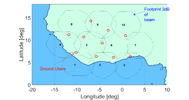
Figure 2: Considered GEO multibeam footprint pattern with $N=10$.

We consider a GEO satellite system with $10$ spot beams serving $10$ users, i.e., $N=10$ and $K=10$, as shown in Fig. 2. Two GWs located in Redu (Belgium), and Betzdorf (Luxembourg) with $(lat,lon)$ coordinates of $(50.002461,5.148105)$ and $(49.692915,6.327135)$ are assumed. Other setting parameters are summarized in Table I. In addition, the efficiency factors of all antennas and HPAs are set at $60\%$ and $\mathbf{A}=\mathbf{I}_{N\times N}$.

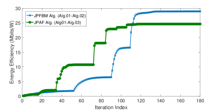
Figure 3: System EE obtained by JPFBM and JPAF algorithms.

First, we investigate the convergence of our proposed algorithms by presenting the system energy efficiency (SEE) results obtained by the joint precoding and FL-beam matching (JPFBM) framework (Alg. 1-2 integration) and the joint precoding with amplify-and-forward (JPAF) framework ( Alg. 1-3 integration) over iterations in Fig. 3. In this simulation, $\bar{P}^{\mathrm{GW}}_{t}=15$ dBW and $\bar{P}^{\mathrm{Sat}}_{n}=5$ dBW, and we consider the total power consumption of the system by setting $\delta^{\sf{GW}}=\delta^{\sf{Sa}}=1$. As observed, the SEEs for both approaches increase and plateau after around $100$ iterations, confirming the convergence of our proposed frameworks. Upon convergence, the JPFBM framework yields a higher SEE compare to the JPAF one.

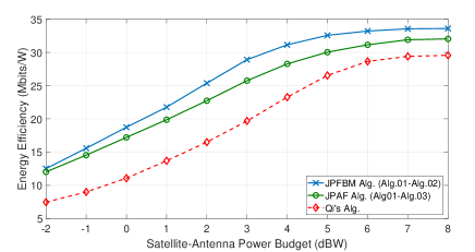
Figure 4: The SEE versus the transmit power budget of each satellite antenna.

Next, Fig. 4 depicts the SEE achieved by our proposed frameworks, as well as of Qi’s method [5], with respect to varying values of $\bar{P}^{\sf{Sa}}_{n}$, the transmission power budget for each satellite antenna. Note that Qi’s work only focuses on satellite power consumption in their SEE formula. To ensure a fair comparison, we set $\mathbf{B}=\left(\mathbf{F}^{H}\mathbf{F}\right)^{-1/2}$ and carry out simple manipulations to estimate the GW power consumption in this approach. Here, $\bar{P}^{\mathrm{GW}}_{t}=15$ dBW. As expected, all three methods can achieve higher SEEs as $\bar{P}^{\sf{Sa}}_{n}$ increases. At the high regime of $\bar{P}^{\sf{Sa}}_{n}$, SEEs of these three tend to saturate due to the limitation in FL transmission. The figure also reveals that our proposed JPFBM and JPAF mechanisms surpass Qi’s algorithm while JPFBM performs better than JPAF.

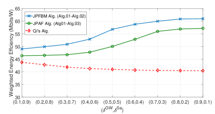
Figure 5: The SWEE versus various values of $(\delta^{\sf{GW}},\delta^{\sf{Sa}})$.

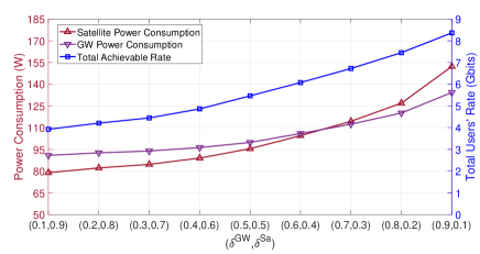
Figure 6: The JPFBM sum rate and power consumption vs. $(\delta^{\sf{GW}},\delta^{\sf{Sa}})$.

Finally, Figs. 5 and 6 illustrate the variations in SWEE, achievable rate, and power consumption of JPFBM mechanism across different values of $(\delta^{\sf{GW}},\delta^{\sf{Sa}})$. In this simulation, we set $\bar{P}^{\mathrm{GW}}_{t}=15$ dBW, $\bar{P}^{\mathrm{Sat}}_{n}=5$ dBW, vary $(\delta^{\sf{GW}},\delta^{\sf{Sa}})$ such that $\delta^{\sf{GW}}+\delta^{\sf{Sa}}=1$. In Fig. 5, the SWEE of our proposed JPFBM and JPAF mechanisms increases while that of Qi’s method decreases as $\delta^{\sf{GW}}$ increases. Once again, our proposed approaches outperform Qi’s method across all $(\delta^{\sf{GW}},\delta^{\sf{Sa}})$ configurations, and the JPFBM mechanism provides superior. These results clearly emphasize the benefits of employing the jointly designed LP and FL-beam matching mechanism in the multi-GW, multi-beam SATCOM systems. In Fig. 6, one depicts that all rate and power consumption enlarge as $\delta^{\sf{GW}}$ increases. These outcomes together with the increasing SWEE shown in Fig. 5 suggest that the user links have a more significant impact on the network performance compared to the FLs in our simulation setting.

V Conclusion

This paper presented a joint optimization framework for energy-efficient precoding and FL-beam matching design in multi-GW, multi-beam bent-pipe SATCOM systems which aims to maximize the SWEE. The technical designs were formulated as a non-convex sparsity problem. Two iterative efficient designs have been proposed to tackle these challenges by employing Dinkelbach’s method and the compress-sensing approach. The simulation results showcased the effectiveness and superiority of the proposed JPFBM and JPAF frameworks over another benchmark method.

References

• [1] M. Centenaro, C. E. Costa, F. Granelli, C. Sacchi, and L. Vangelista, “A survey on technologies, standards and open challenges in satellite iot,” IEEE Communications Surveys & Tutorials, vol. 23, 2021.
• [2] Y. Liu, C. Li, J. Li, and L. Feng, “Robust Energy-Efficient Hybrid Beamforming Design for Massive MIMO LEO Satellite Communication Systems,” IEEE Access, vol. 10, pp. 63 085–63 099, 2022.
• [3] V. N. Ha, T. T. Nguyen, E. Lagunas, J. C. Merlano Duncan, and S. Chatzinotas, “GEO payload power minimization: Joint precoding and beam hopping design,” pp. 6445–6450, 2022.
• [4] S. Chatzinotas, G. Zheng, and B. Ottersten, “Energy-efficient mmse beamforming and power allocation in multibeam satellite systems,” in 2011 Conference Record of the Forty Fifth Asilomar Conference on Signals, Systems and Computers (ASILOMAR), 2011, pp. 1081–1085.
• [5] C. Qi, H. Chen, Y. Deng, and A. Nallanathan, “Energy efficient multicast precoding for multiuser multibeam satellite communications,” IEEE Wireless Communications Letters, vol. 9, no. 4, pp. 567–570, 2020.
• [6] T. S. Abdu, S. Kisseleff, E. Lagunas, S. Chatzinotas, and B. Ottersten, “Energy efficient sparse precoding design for satellite communication system,” in 2022 IEEE 96th Vehicular Technology Conference (VTC2022-Fall), 2022, pp. 1–6.
• [7] V. Joroughi, M. A. Vazquez, and A. I. Perez-Neira, “Precoding in multigateway multibeam satellite systems,” IEEE Transactions on Wireless Communications, vol. 15, no. 7, pp. 4944–4956, 2016.
• [8] T. Delamotte and A. Knopp, “Smart diversity through mimo satellite $q/v$-band feeder links,” IEEE Transactions on Aerospace and Electronic Systems, vol. 56, no. 1, pp. 285–300, 2020.
• [9] H. Yan, S. Ramesh, T. Gallagher, C. Ling, and D. Cabric, “Performance, power, and area design trade-offs in millimeter-wave transmitter beamforming architectures,” IEEE Circuits and Systems Magazine, vol. 19, no. 2, pp. 33–58, 2019.
• [10] W. Dinkelbach, “On nonlinear fractional programming,” Manage. Sci., vol. 13, no. 7, p. 492–498, mar 1967.
• [11] “Hitec-lm-06: 6,8m limited-motion satellite ground antenna system,” HITEC Luxembourg S.A., Tech. Rep., June 2020.