Implicit Counterfactual Data Augmentation
for Deep Neural Networks

Abstract

Machine-learning models are prone to capturing the spurious correlations between non-causal attributes and classes, with counterfactual data augmentation being a promising direction for breaking these spurious associations. However, explicitly generating counterfactual data is challenging, with the training efficiency declining. Therefore, this study proposes an implicit counterfactual data augmentation (ICDA) method to remove spurious correlations and make stable predictions. Specifically, first, a novel sample-wise augmentation strategy is developed that generates semantically and counterfactually meaningful deep features with distinct augmentation strength for each sample. Second, we derive an easy-to-compute surrogate loss on the augmented feature set when the number of augmented samples becomes infinite. Third, two concrete schemes are proposed, including direct quantification and meta-learning, to derive the key parameters for the robust loss. In addition, ICDA is explained from a regularization aspect, with extensive experiments indicating that our method consistently improves the generalization performance of popular depth networks on multiple typical learning scenarios that require out-of-distribution generalization.

I Introduction

Deep learning models are supposed to learn invariances and make stable predictions based on some right causes. However, models trained with empirical risk minimization are prone to learning spurious correlations and suffer from high generalization errors when the training and test distributions do not match [1, 2]. For example, dogs are mostly on the grass in the training set. Thus, a dog in the water can easily be misclassified as a “drake” due to its rare scene context (“water”) in the “dog” class, as illustrated in Fig. 1. A promising solution for improving the models’ generalization and robustness is to learn causal models [3], as if a model can concentrate more on the causal correlations but not the spurious associations between non-causal attributes and classes, stable and exact predictions are more likely.

Counterfactual augmentation has become popular for causal models because of its clear explanation and being model-agnostic. For instance, Lu et al. [4] and He et al. [5] augmented the data effectively by swapping identity pronouns in texts. Moreover, Chang et al. [6] introduced two new image generation procedures that included counterfactual and factual data augmentations to reduce spuriousness between backgrounds of images and labels, achieving higher accuracy in several challenging datasets. Mao et al. [2] utilized a novel strategy to learn robust representations that steered generative models to manufacture interventions on features caused by confounding factors. Nevertheless, the methods presented above suffer from several shortcomings. Specifically, it is not trivial to explicitly find all confounding factors, and the training efficiency will decline as excess augmented images are involved in training.

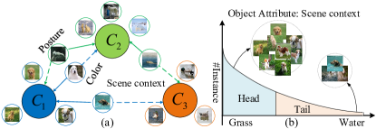
Figure 1: (a): Illustration for images affected by spurious correlations due to rare attributes (e.g., posture, color, and scene context). $C_{1}$, $C_{2}$, and $C_{3}$ are the dog, polar bear, and drake classes, respectively. The solid line connects the sample’s ground-truth class, and the dotted line connects the class with a spurious correlation with the sample. (b): Illustration for attribute imbalance.

It should be mentioned that implicit data augmentation settles the inefficiency of explicit augmentation by avoiding the generation of excess samples. ISDA [7] conducts a pioneering study on implicit data augmentation, which is inspired by the observation that the deep features in a network are usually linearized. Then, it translates samples along the semantic directions in the feature space based on an assumed class-wise augmentation distribution. By deriving an upper bound on the expected cross-entropy (CE) loss, ISDA enables optimization of only the upper bound to achieve data augmentation in an efficient way. Moreover, MetaSAug [8] innovatively applies the idea of ISDA to the long-tailed recognition, which does not modify the augmentation distribution of ISDA but optimizes the covariance matrices using metadata, yielding good performance on imbalanced data. Besides, RISDA [9] constructs novel augmentation distributions of tail classes by mixing the information from relevant categories, thus more effectively enriching samples in tail categories. However, these methods adopt purely class-wise semantic augmentation strategies, and thus samples in the same class have identical augmentation distributions that are inaccurate. Fig. 1(a) illustrates samples in the same class that may be negatively influenced by different attributes (or classes), where an ideal augmentation strategy should consider these sample-wise non-causal attributes. Additionally, these methods adopt the same augmentation strength for each instance, ignoring that inappropriate distributions (e.g., imbalanced label and attribute distributions) also lead to spurious associations.

Spurred by the above deficiencies, this study proposes a sample-wise implicit counterfactual data augmentation (ICDA) method that can translate each sample corresponding to semantic and counterfactual transformations in the feature space. To ensure that the counterfactual transformations are meaningful, each sample’s augmentation distribution and strength are determined based on class-wise statistical information and the degree of spurious correlation between the sample and each category. Then, we verify that ICDA can be implemented by optimizing a new robust surrogate loss enhancing efficiency. Furthermore, meta-learning is introduced to learn key parameters in ICDA, which is analyzed and compared against existing methods in a unified regularization perspective, revealing that it enforces extra intra-class compactness by reducing the classes’ mapped variances and encourages larger sample margins and class-boundary distances.

Extensive experiments verify that ICDA consistently achieves state-of-the-art performance in several typical learning scenarios requiring the models to be robust and presenting a high generalization ability. Furthermore, the visualization results indicate that ICDA generates more diverse and meaningful counterfactual images with rare attributes, helping models break spurious correlations and affording stable predictions for the right reasons.

II Related Work

II-A Causal Inference and Counterfactual

Causal inference [10] has been widely adopted in psychology, politics, and epidemiology for years [11, 12], serving as an explanatory framework and providing solutions to achieve the desired objectives by pursuing the causal effect. Recently, it has also attracted increasing attention in computer vision society [13, 14, 15, 16, 17, 18] for removing the dataset bias in domain-specific applications. Among the causal inference approaches, counterfactual has been widely investigated to explain and remove spurious associations [2, 6, 1, 3, 4] and achieved promising performance. Counterfactuals describe situations that did not actually occur, allowing for comparison between actual and hypothetical scenarios.

II-B Data Augmentation

Counterfactual and implicit semantic augmentation strategies are reviewed here. Counterfactual augmentation generates hypothetical samples (i.e., counterfactuals) by making small changes to the original samples, which can be divided into hand-crafted [6, 5] and using causal generative models [19, 20], demonstrating competitive performance. However, explicitly finding the non-causal attributes is challenging and training models based on the augmented data is inefficient. Implicit semantic data augmentation overcomes the inefficiency of explicit data augmentation approaches [7, 8, 9] as it does not generate excess samples and achieves the effect of augmentation only through optimizing the surrogate loss, which is thus efficient. However, implicit data augmentation can not help overcome spurious associations. Besides, all samples or samples in the same class are treated equally in existing approaches, which is naturally not optimal.

II-C Logit Adjustment (LA)

Logit vectors are the outputs of the final feature encoding layer in most deep neural networks. LA approaches introduce some perturbation terms to logits to enhance the robustness of models, first proposed in face recognition [21, 22] to enlarge inter-class distance and intra-class compactness. Nowadays, data augmentation [7, 9] and long-tailed classifications [23, 24, 25] also implicitly or explicitly utilize LA.

III Casual Graph

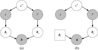
Figure 2: (a): The original casual graph. (b): The causal graph after intervention on $\boldsymbol{h}_{z}$. Interventional nodes are squared. Gray (white) nodes mean the observed (latent) variables.

We constructed our causal graph in a similar manner to Ilse et al. [26], who provided a thorough explanation for the effectiveness of data augmentation through causal concepts. As illustrated in Fig. 2, $\mathcal{C}$ represents a confounder, which is an extraneous variable that is related to both the exposure and outcome of interest, but is not on the causal path between them; $z$ refers to non-causal attributes such as background, color, and shape; $y$ is the target; $\boldsymbol{h}_{z}$ means the non-causal features caused by $z$; and $\boldsymbol{h}_{y}$ is the causal features caused by $y$. The variables in the graph follow

$$z: =f_{z}(\mathcal{C}),$$ (1)

$$y: =f_{y}(\mathcal{C}),$$

$$\boldsymbol{h}_{z}: =f_{H_{z}}(z),$$

$$\boldsymbol{h}_{y}: =f_{H_{y}}(y),$$

$$\boldsymbol{h}: =f_{H}(\boldsymbol{h}_{z},\boldsymbol{h}_{y}),$$

where $\boldsymbol{h}$ is the deep feature of sample $\boldsymbol{x}$. The confounding variable $\mathcal{C}$ creates a backdoor path $z\!\leftarrow\!\mathcal{C}\!\rightarrow\!y$, allowing $z$ to affect $y$ through the back door. The objective is to predict $y$ from $\boldsymbol{h}$, which is anti-causal itself. Since $z$ and $y$ are correlated, the machine learning model is likely to rely on non-causal attributes to predict $y$. Moreover, assuming the correlation between $z$ and $y$ is spurious, it will not hold in general. Thus, a machine learning model that depends on non-causal features $\boldsymbol{h}_{z}$, caused by $z$, will have poor generalization to unseen environments. In the case of animal classification in images [26], $\mathcal{C}$ could represent a common cause of the type of animal and the landscape in an image. For instance, the confounder may be the country where a specific image was captured. In Switzerland, for example, we are more likely to see a cow grazing in a green pasture than a camel in a desert.

The most common approach to address spurious correlations between $z$ and $y$ is to intervene on $z$, which would make $z$ and $y$ independent, i.e., $p(y|\text{do}(z))=p(y)$. For instance, in the context of animals and landscapes, intervening in the background $z$ could involve physically relocating a cow to a desert. Another manner proposed by Ilse et al. [26] to break the spurious correlations between $z$ and $y$ involves intervening on $\boldsymbol{h}_{z}$, since $z$ affects $\boldsymbol{h}$ only indirectly via $\boldsymbol{h}_{z}$. The casual graph after intervening on $\boldsymbol{h}_{z}$ is shown in Fig. 2(b). The intervention, $\rm{do}(\boldsymbol{h}_{z})$, would need to be performed during the process of augmenting the sample features.

By intervening $\boldsymbol{h}_{z}$ resulting from $z$, we ensure that the target variable $y$ and features $\boldsymbol{h}_{y}$ remain unchanged. Once data augmentation is performed, the pairs $(\boldsymbol{h}_{\rm{aug}},y)$ should resemble samples from the interventional distribution $p(\boldsymbol{h},y|\rm{do}(\boldsymbol{h}_{z}))$. Additionally, each augmented feature $\boldsymbol{h}_{\rm{aug}}$ can be viewed as a counterfactual. Therefore, our objective is to design the augmentation function $\boldsymbol{h}_{\text{aug}}=\text{aug}(\boldsymbol{h})$ as a transformation applied to $\boldsymbol{h}$, such that it mimics an intervention on $\boldsymbol{h}_{z}$. According to the intervention-augmentation equivariance [26], we have

$$\boldsymbol{h}_{\text{aug}}\!=\!\text{aug}(\boldsymbol{h})\!=\!\text{aug}(f_{H}(\boldsymbol{h}_{z},\boldsymbol{h}_{y}))\!=\!f_{H}(\text{do}(\boldsymbol{h}_{z}),\boldsymbol{h}_{y}).$$ (2)

Eq. (2) illustrates an ideal augmentation manner, and our proposed method aims to achieve this in a reasonable way.

IV Implicit Counterfactual Data Augmentation

Notation. Consider training a network $G$ with weights $\boldsymbol{W}$ on a training set $D^{\text{train}}\!=\!\{(\boldsymbol{x}_{i},y_{i})\}_{i=1}^{N}$, where $y_{i}\!\in\!\{1,\!\cdots,\!C\}$ is the label of the $i$-th sample $\boldsymbol{x}_{i}$ over $C$ classes. Let the $H$-dimensional vector $\boldsymbol{h}_{i}\!=\!G(\boldsymbol{x}_{i},\boldsymbol{W})$ denote the deep feature of $\boldsymbol{x}_{i}$ learned by $G$. Let $\boldsymbol{u}_{i}\!=\!f(\boldsymbol{h}_{i})\!=\!\boldsymbol{w}\boldsymbol{h}_{i}\!+\!\boldsymbol{b}$ denote the logit vector, $\boldsymbol{w}\!=\![\boldsymbol{w}_{1},\!\cdots,\!\boldsymbol{w}_{C}]^{\top}\!\in\!\mathrm{R}^{C\times H}$, and $\boldsymbol{b}\!=\![{b}_{1},\!\cdots,\!{b}_{C}]^{\top}\!\in\!\mathrm{R}^{C}$. Let $\boldsymbol{\mu}_{c}$ and $\Sigma_{c}$ be the mean and covariance matrix of the features for class $c$. $\mathcal{N}(\boldsymbol{\mu},\Sigma)$ means a multivariate normal distribution with mean vector $\boldsymbol{\mu}$ and covariance matrix $\Sigma$.

IV-A Our Sample-wise Augmentation Strategy

The developed strategy augments data to implement both content and distribution counterfactuals. Regarding content counterfactual, we intervene in the non-causal attributes spuriously correlated with other classes to enhance their independence from confounders while preserving the core object features. Therefore, if attributes in sample $\boldsymbol{x}_{i}$ (e.g., background) are spuriously associated with category $c$, the augmented data for $\boldsymbol{x}_{i}$ are supposed to contain information of class $c$. Distribution counterfactual means that if there are spurious correlations brought by certain class and attribute distributions for partial or a single sample, the distributions for the augmented samples should be opposite to the class/attribute distributions. However, existing counterfactual augmentation studies overlook the distribution counterfactual, while samples in tail classes or those with rare attributes are most likely to be spuriously correlated due to the class and attribute imbalance [27]. Fig. 1(a) illustrates samples with rare scene contexts and postures that are spuriously correlated with the negative classes containing quite similar contexts and colors. Thus, these samples should be augmented more to counter the class and attribute distributions.

Naturally, different samples will have varying augmentation distributions as the spurious correlations between samples and categories are sample-wise and have unequal augmentation strengths as the samples in tail classes or those with rare attributes should augment more. Fig. 3 (left) highlights that the existing augmentation approaches ignore the relationship between samples and the other category and all samples are treated equally, prohibiting a well-adjusted distribution.

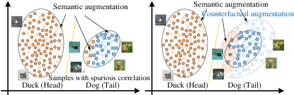
Figure 3: Left: Diagram for ISDA, which only conducts semantic augmentation and treats all samples equally. Right: Diagram for ICDA, containing semantic and counterfactual augmentations. Samples in the tail class (Dog) and those with rare attributes (yellow ones in Dog class) are augmented most. The two axes mean the dimensions of the 2D feature space, in which each sample is represented by a dot or square. Solid and transparent samples are the original and augmented ones. Samples in the same red circle are augmented from the same sample. The augmentation strength is determined by the degree of spurious associations.

Following ISDA, our sample-wise augmentation strategy augments samples in the feature space, which comprises two key parts. The first part refers to the sample-wise augmentation distribution, which generates both meaningful semantic and counterfactual sample features by adopting the ground-truth class information and the weighted information of the other classes. In this way, when $\boldsymbol{h}_{i}$ is augmented to class $c$ ($\neq y_{i}$), the perturbation vector is randomly sampled from a multivariate normal distribution $\mathcal{N}(\boldsymbol{0}+\alpha_{i,c}\boldsymbol{\mu}_{c},\Sigma_{y_{i}}+\alpha_{i,c}\Sigma_{{c}})$, where $\alpha_{i,c}(\geq 0)$ is determined by the degree of the spurious association between $\boldsymbol{x}_{i}$ and class $c$, which controls the tradeoff between the strengths of semantic and counterfactual data augmentations. Following ISDA, if the perturbation vector is sampled from $\mathcal{N}(\boldsymbol{0},\Sigma_{y_{i}})$, then the sample is semantically augmented. In another case, if it is sampled from $\mathcal{N}(\boldsymbol{\mu}_{c},\Sigma_{c})$, then the sample is counterfactually augmented as the sample is spuriously correlated with class $c$. In fact, all non-causal attributes for an instance are involved in our predefined augmentation distributions for this sample which contain the information of the instance’s spuriously correlated classes.

The second part refers to the augmentation strength, or the number of augmented samples $\tilde{M}_{i,c}$ for sample $\boldsymbol{x}_{i}$ to class $c$. It is assumed to follow $\tilde{M}_{i,c}=(M{\alpha_{i,c}})/{\pi_{y_{i}}}$, where $\pi_{y_{i}}$ denotes the proportion of class $y_{i}$; $M$ is the basic quantity of the augmented pieces for all samples which is a constant. Therefore, the higher the degree of the spuriousness between $\boldsymbol{x}_{i}$ and class $c$ and the smaller the $\pi_{y_{i}}$, the larger the number ($\tilde{M}_{i,c}$) of samples will be augmented from $\boldsymbol{x}_{i}$ to class $c$. Fig. 3 (right) presents that samples in the tail class and the ones most spuriously correlated with attributes of the other class are augmented most.

During training, $C$ feature means and covariance matrices are computed, one for each class. Given that the estimated statistics information in the first few epochs is not quite informative, we add a scale parameter $\lambda\!=\!(t/T)\!\times\!\lambda^{0}$ before the estimated $\boldsymbol{\mu}$ and $\Sigma$, where $t$ and $T$ refer to the numbers of the current and total iterations. The augmented feature ${\boldsymbol{h}}_{i,c}$ for $\boldsymbol{h}_{i}$ to class $c$ is obtained by translating $\boldsymbol{h}_{i}$ along a random direction sampled from the above multivariate normal distribution. Equivalently, we have $\boldsymbol{{h}}_{i,c}\!\sim\!\mathcal{N}(\boldsymbol{{h}}_{i}\!+\!\lambda\alpha_{i,c}\boldsymbol{\mu}_{c},\lambda(\Sigma_{y_{i}}\!+\!\alpha_{i,c}\Sigma_{{c}}))$.

Notably, the underlying augmentation strategy of ICDA has distinct differences from current implicit semantic augmentation methods, including ISDA, RISDA, and MetaSAug:

• Their motivations are different. ICDA aims to generate more data for content and distribution counterfactuals and thus breaks spurious correlations, while the existing methods generate diverse semantic data.

• Their granularities are different. The augmentation strategy in ICDA is sample-wise, which is fine-grained and pinpoint, while current schemes involve class-wise strategies. Additionally, ICDA utilizes the information in the spuriously correlated classes, while ISDA and MetaSAug only use that in the ground-truth class.

• ICDA highlights the augmentation strength, which is crucial in an augmentation strategy as inappropriate class and attribute distributions always cause spuriousness. However, it is overlooked by the existing methods.

Section VI further demonstrates ICDA’s superiority against current methods from a regularization perspective.

IV-B New Loss under Implicit Augmentation

Assume that each feature $\boldsymbol{h}_{i}$ is augmented to class ${c}$ for $\tilde{M}_{i,c}$ times by sampling from the corresponding distribution, forming an augmented feature set $\{\{\boldsymbol{h}_{i,c}^{1},\cdots,\boldsymbol{h}_{i,c}^{\tilde{M}_{i,c}}\}_{c=1,c\neq y_{i}}^{C}\}_{i=1}^{N}$. The corresponding CE loss is

where $\tilde{M}\!=\!\sum_{i=1}^{N}\!\sum_{c=1,c\neq y_{i}}^{C}\!\tilde{M}_{i,c}$ and $f_{j}(\boldsymbol{h}_{i,c}^{k})=\boldsymbol{w}_{j}^{\top}\boldsymbol{h}_{i,c}^{k}+{b}_{j}$. Let $M$ in $\tilde{M}_{i,c}$ grow to infinity. Then, the expected loss is

where $\tilde{N}_{i,c}\!=\!{\alpha_{i,c}}/{\pi_{y_{i}}}$ and $\tilde{N}\!=\!\sum_{i=1}^{N}\sum_{c=1,c\neq y_{i}}^{C}\tilde{N}_{i,c}$. Following the similar inference strategy in ISDA, a more easy-to-compute surrogate loss is derived for Eq. (4), leading to a highly efficient implementation:

where $P_{c,{i}}\!=\!\Delta\boldsymbol{w}_{c,{y_{i}}}(\Sigma_{y_{i}}\!+\!\sum_{j=1,j\neq y_{i}}^{C}\hat{\alpha}_{i,j}\Sigma_{{j}})\Delta\boldsymbol{w}_{{c},y_{i}}^{\top}$ and $Q_{c,{i}}\!=\!\Delta\boldsymbol{w}_{c,{y_{i}}}\sum_{j=1,j\neq y_{i}}^{C}\hat{\alpha}_{i,j}\boldsymbol{\mu}_{j}$, in which $\Delta\boldsymbol{w}_{c,y_{i}}\!=\!\boldsymbol{w}_{c}^{\top}\!-\!\boldsymbol{w}_{y_{i}}^{\top}$ and $\hat{\alpha}_{i,j}={\alpha_{i,j}}/{(C\!-\!1)}$. In addition, $\alpha_{i}\!=\!\sum_{j=1,j\neq y_{i}}^{C}{\hat{\alpha}}_{i,j}$. The inference details are presented in Appendix A.

Although $\mathcal{L}_{s}(\boldsymbol{w},\boldsymbol{b},\boldsymbol{W})$ can be directly utilized during training, a more effective loss is leveraged after adopting the two following modifications: (1) Inspired by the manner in LA [24], the class-wise weight $1/\pi_{y_{i}}$ is replaced by a perturbation term on logits. (2) We only retain the term $\Delta\boldsymbol{w}_{{c},y_{i}}\hat{\alpha}_{i,c}\boldsymbol{\mu}_{c}$ in $Q_{c,{i}}$. A detailed reasoning for the proposed variation is presented in Section VI. Accordingly, the final ICDA training loss becomes

where $\delta_{c,{i}}\!=\!\log({\pi_{c}}/{\pi_{y_{i}}})$ and $\beta$ is a hyperparameter which is fixed as $0.1$ in our experiments. When ${\lambda}\!=\!\beta\!=\!0$, our method can be reduced to LA. Additionally, for $\hat{\alpha}_{i,c}\!=\!\beta\!=\!0$ and balanced classes, ICDA degenerates to ISDA. The first two terms in $\hat{\phi}_{i,c}$ are sample-wise compared with those in RISDA.

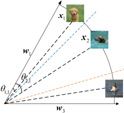
Figure 4: Illustration for the angle between sample feature and weight vector.

V Learning with ICDA

In realization, $\boldsymbol{\mu}_{c}$, $\Sigma_{c}$, and $\alpha_{i,c}$ in the ICDA training loss should be prefixed, resulting in two manners according to the existence of metadata.

V-A Direct Quantification-based Manner

The spurious correlation between sample $\boldsymbol{x}_{i}$ and category $c$ can be directly quantified by the angle ($\theta_{i,c}$) between $\boldsymbol{h}_{i}$ and the weight vector $\boldsymbol{w}_{c}$ of class $c$. Naturally, the larger the spurious correlation between $\boldsymbol{h}_{i}$ and class $c$, the smaller the $\theta_{i,c}$ and the larger the $\cos\theta_{i,c}$. An illustration is presented in Fig. 4. Samples $\boldsymbol{x}_{1}$ and $\boldsymbol{x}_{2}$ both belong to class $C_{1}$. Nevertheless, $\theta_{2,1}$ is larger than $\theta_{1,1}$ as $\boldsymbol{x}_{2}$ is more spuriously correlated with class $C_{3}$.

Since $\alpha_{i,c}$ is determined by the degree of spurious correlation between $\boldsymbol{x}_{i}$ and class $c$, it should be positively correlated with $\cos\theta_{i,c}$. Moreover, only when the direction of $\boldsymbol{h}_{i}$ is partially consistent with that of $\boldsymbol{w}_{c}$ (i.e., $\theta_{i,c}\!<\!90^{\circ}$), the information of class $c$ should be utilized to augment sample $\boldsymbol{x}_{i}$. Thus, we denote $\alpha_{i,c}\!=\!\max(\cos\theta_{i,c},0)$, where a larger $\alpha_{i,c}$ value means a larger counterfactual augmentation strength. Then, we have $\alpha_{i}\!\propto\!\sum_{c\neq y_{i}}\max(\cos\theta_{i,c},0)$. Nevertheless, quantifying $\alpha_{i}$ through angle $\theta_{i,y_{i}}$ is more direct. If $\boldsymbol{x}_{i}$ is notably influenced by the spurious correlations with other classes, then $\theta_{i,y_{i}}$ will be large and $\cos\theta_{i,y_{i}}$ will be small. Thus, $\alpha_{i}$ should be negatively correlated with $\cos\theta_{i,y_{i}}$. Meanwhile, the value range of $\alpha_{i}$ is restricted to $[0,1]$. Therefore, we let $\alpha_{i}={(1-\cos\theta_{i,y_{i}})}/{2}$. This manner is empirically verified to be more effective. The feature means $\boldsymbol{\mu}$ and covariance matrices $\Sigma$ of classes are computed online by aggregating statistics from all mini-batches following ISDA [7], which is given in Appendix B.

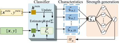
Figure 5: Overall structure of Meta-ICDA.

V-B Meta-learning-based Manner (Meta-ICDA)

If metadata are available, the extent a sample is affected by spurious correlation can be better determined by training a strength generation network, with its input involving ten training characteristics of samples $\boldsymbol{\zeta}_{i}$, including loss, margin, uncertainty, etc., denoted by ${\zeta}_{{i},1},\cdots,{\zeta}_{{i},10}$. Details for the extracted training characteristics are presented in Appendix C. In this study, the network is a two-layer MLP and its output is the augmentation strength $\alpha_{i}$. Thus, we have $\alpha_{i}=\text{MLP}(\boldsymbol{\zeta}_{i})$. Considering that the geodesic distance between the sample and other classes can well measure their correlation [28], $\alpha_{i,c}$ is still calculated by $\max(\cos\theta_{i,c},0)$. Like MetaSAug, the estimated covariance matrices and the feature means are optimized on metadata because biased training data (e.g., imbalanced and noisy data) may not estimate the statistical information well. Fig. 5 illustrates the framework of Meta-ICDA, which includes three main parts: the classifier network, the strength generation network, and the characteristics extraction module. We utilize an online meta-learning-based learning strategy inspired by MAML [29] to alternatively update the parameters of the classifier and the strength generation network.

To ease this paper’s notation, the deep classifier network’s parameters of $\boldsymbol{W}$ and $\boldsymbol{w}$ are denoted as $\tilde{\boldsymbol{W}}$. The deep classifier which includes both feature extractor $G$ and classifiers is denoted as $\tilde{f}$. The parameters in the strength generation network are $\boldsymbol{\Omega}$. The small metadata set is denoted as $D^{\text{meta}}=\{\boldsymbol{x}_{i}^{\rm{meta}},y_{i}^{\rm{meta}}\}_{i=1}^{B}$, where $B\leq N$.

Algorithm 1 Meta-ICDA

Input: Training data $D^{\text{train}}$, metadata ${D}^{\text{meta}}$, batch size $n$, meta batch size $m$, number of iterations $T$.
Output: Learned $\tilde{\boldsymbol{W}}$ and $\boldsymbol{\Omega}$.

1:  Initialize $\tilde{\boldsymbol{W}}^{(1)}$ and $\boldsymbol{\Omega}^{(1)}$;

2:  for $t=1$ to $T$ do

3:     Sample ${(\boldsymbol{x}_{i},{y}_{i})}_{i=1}^{n}$ from $D^{\text{train}}$;

4:     Sample ${(\boldsymbol{x}^{\text{meta}}_{i},{y}^{\text{meta}}_{i})}_{i=1}^{m}$ form $D^{\text{meta}}$;

5:     Calculate current feature means $\boldsymbol{\mu}^{(t)}$ and covariance matrices $\Sigma^{(t)}$;

6:     Formulate $\overline{\tilde{\boldsymbol{W}}}^{(t)}(\boldsymbol{\Omega})$ by Eq. (7);

7:     Update $\boldsymbol{\Omega}^{(t+1)}$ by Eq. (8);

8:     Update $\boldsymbol{\mu}^{(t+1)}$ and $\Sigma^{(t+1)}$ by Eqs. (9) and (10);

9:      Update $\tilde{\boldsymbol{W}}^{(t+1)}$ by Eq. (11);

10:  end for

During this process, first, the parameter of the deep classifier $\tilde{f}$, that is $\tilde{\boldsymbol{W}}$, is formulated. We utilize the stochastic gradient descent (SGD) optimizer to optimize the training loss on a minibatch of training samples $\{\boldsymbol{x}_{i},{y}_{i}\}_{i=1}^{n}$ in each iteration, where $n$ is the size of the mini-batch. Thus, $\tilde{\boldsymbol{W}}$ is formulated by the following equation:

where $\eta_{1}$ is the step size. After extracting the training characteristics from the classifier, the parameter of the strength generation network $\boldsymbol{\Omega}$ can be updated on a minibatch of metadata as follows:

where $m$ and $\eta_{2}$ are the minibatch size of metadata and the step size, respectively. At the same time, the feature means and covariance matrices for all classes are optimized based on the metadata:

${\Sigma}^{(t)}$ and $\boldsymbol{\mu}^{(t)}$ refer to the covariance matrices and feature means of all classes in step $t$, respectively. Finally, the parameters of the classifier network can be updated with the obtained augmentation strengths $\alpha_{i}^{(t+1)}$:

The steps of Meta-ICDA are presented in Algorithm 1.

VI Explanation in Regularization View

This section conducts a deeper analysis considering regularization and reveals the ICDA’s superiority against three advanced approaches: LA, ISDA, and RISDA. To our knowledge, this is the first time regularization is used to explain these methods.

TABLE I: Regularization terms and reflected generalization factors of the four algorithms (LA, ISDA, RISDA, and ICDA).

Method	Regularization term	Generalization factor
LA	${R_{LA}}{\rm{=}}\sum_{i=1}^{N}{\sum_{c\neq{y_{i}}}{{{q}_{i,c}}\delta_{c,{i}}}}$	✓Class-wise margin
ISDA	${R_{ISDA}}{\rm{=}}\frac{\lambda}{2}\sum_{i=1}^{N}{\sum_{c\neq{y_{i}}}{{{q}_{i,c}}{\Delta\boldsymbol{w}_{c,y_{i}}\Sigma_{y_{i}}\Delta\boldsymbol{w}_{c,y_{i}}^{\top}}}}$	✓Intra-class compactness
RISDA	${R_{RISDA}}{\rm{=}}\sum_{i=1}^{N}{\sum_{c\neq{y_{i}}}{{{q}_{i,c}}[\alpha\Delta{\boldsymbol{w}_{c,y_{i}}}\sum_{j=1,j\neq{y_{i}}}^{C}{{\varepsilon_{y_{i},j}}{\boldsymbol{\mu}_{j}}}+\beta\Delta{\boldsymbol{w}_{c,y_{i}}}({\Sigma_{{y_{i}}}}+\sum_{j=1,j\neq{y_{i}}}^{C}{{\varepsilon_{y_{i},j}}}{\Sigma_{j}})\Delta\boldsymbol{w}_{c,y_{i}}^{\top}]}}$	✓Intra-class compactness ✓Class-boundary distance
ICDA	${R_{ICDA}}{\rm{=}}\sum\limits_{i=1}^{N}\{{\sum\limits_{c\neq{y_{i}}}{{{q}_{i,c}}[\delta_{c,{i}}+\frac{{\lambda}}{2}{\Delta\boldsymbol{w}_{c,y_{i}}(\Sigma_{y_{i}}\!+\!\sum\limits_{j=1,j\neq y_{i}}^{C}\hat{\alpha}_{i,j}\Sigma_{{j}})\Delta\boldsymbol{w}_{c,y_{i}}^{\top}}}}+{\lambda}\Delta{\boldsymbol{w}_{c,y_{i}}}{\hat{\alpha}_{i,c}}{\boldsymbol{\mu}_{c}}]-\beta{\alpha_{i}}{{q}_{i,{y_{i}}}}\}$	✓Sample-wise/class-wise margin ✓Intra-class compactness ✓Class-boundary distance

Using the first-order Taylor expansion of the loss, we have

where $\boldsymbol{q}\!=\!\text{softmax}(\boldsymbol{u})$ and $\boldsymbol{y}$ is the one-hot label. Considering $R\!=\!(\boldsymbol{q}\!-\!\boldsymbol{y})^{\top}\Delta\boldsymbol{u}$, the underlying regularizers of all approaches can be derived. The deviation process is presented in Appendix D. The regularizers and the factors affecting the generalization capability are summarized in Table I.

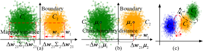
Figure 6: Illustrations for the mapped variance (a) and class-boundary distance (b). (c) demonstrates that different samples in the same category should also have distinct augmentation directions.

$R_{{LA}}$ imposes greater punishment on the predictions ${q}_{i,c}$ ($c\!\neq\!y_{i}$) with a large $\delta_{c,{i}}$, improving their classification performance. Obviously, tail classes benefit more from LA. Thus, LA is prevalent in handling class imbalance.

$R_{{ISDA}}$ contains $\Delta\boldsymbol{w}_{c,y_{i}}\Sigma_{y_{i}}\Delta\boldsymbol{w}_{c,y_{i}}^{\top}$, and we prove that it is the mapped variance from samples of class $y_{i}$ to the normal vector of the boundary between classes $y_{i}$ and $c$ (Fig. 6(a)).

Proof.

If feature $\boldsymbol{h}$ is on the boundary, we have

$$\boldsymbol{w}^{\top}_{c}\boldsymbol{h}+{b}_{c}=\boldsymbol{w}_{y_{i}}^{\top}\boldsymbol{h}+{b}_{y_{i}}.$$ (13)

Then, we know that the boundary between classes $c$ and $y_{i}$ is

$$\Delta\boldsymbol{w}_{c,y_{i}}\boldsymbol{h}+\Delta{b}_{c,y_{i}}=0,$$ (14)

and $\Delta\boldsymbol{w}_{c,y_{i}}\!=\!\boldsymbol{w}_{c}^{\top}\!-\!\boldsymbol{w}_{y_{i}}^{\top}$ refers to the normal direction of the boundary between classes $y_{i}$ and $c$. Thus, the value of the mapping $\Pi(\boldsymbol{h})$ of feature $\boldsymbol{h}$ in class $y$ to $\Delta\boldsymbol{w}_{c,y_{i}}$ is

$$\Pi(\boldsymbol{h})=\Delta\boldsymbol{w}_{c,y_{i}}\boldsymbol{h}+\Delta{b}_{c,y_{i}}.$$ (15)

The (expected) variance of $\Pi(\boldsymbol{h})$ for $y\!=\!y_{i}$ denoted by $\Lambda_{y_{i}}$ is as follows:

$$\Lambda_{c,y_{i}} =\mathrm{E}_{\Pi(\boldsymbol{h}):y=y_{i}}(\Pi(\boldsymbol{h})-\overline{\Pi(\boldsymbol{h})})(\Pi(\boldsymbol{h})-\overline{\Pi(\boldsymbol{h})})^{\top}$$ (16)

$$=\mathrm{E}_{\boldsymbol{h}:y=y_{i}}[\Delta\boldsymbol{w}_{c,y_{i}}(\boldsymbol{h}-\overline{\boldsymbol{h}})(\boldsymbol{h}-\overline{\boldsymbol{h}})^{\top}\Delta\boldsymbol{w}^{\top}_{c,y_{i}}]$$

$$=\Delta\boldsymbol{w}_{c,y_{i}}\mathrm{E}_{\boldsymbol{h}:y=y_{i}}[(\boldsymbol{h}-\overline{\boldsymbol{h}})(\boldsymbol{h}-\overline{\boldsymbol{h}})^{\top}]\Delta\boldsymbol{w}^{\top}_{c,y_{i}}$$

$$=\Delta\boldsymbol{w}_{c,y_{i}}\Sigma_{y_{i}}\Delta\boldsymbol{w}^{\top}_{c,y_{i}},$$

where $\overline{\Pi(\boldsymbol{h})}=\mathrm{E}_{\Pi(\boldsymbol{h}):y=y_{i}}[\Pi(\boldsymbol{h})]$ and $\overline{\boldsymbol{h}}=\mathrm{E}_{\boldsymbol{h}:y=y_{i}}[\boldsymbol{h}]$. ∎

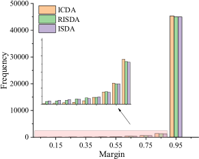
Figure 7: Distributions of the margin values of models trained with the ISDA, RISDA, and ICDA losses.

This term will force the model to decrease the mapped variances of class $y_{i}$ towards the normal vectors of boundaries related to $y_{i}$, and thus increase intra-class compactness. This explains why ISDA performs well on standard datasets. However, as head categories have large training sizes, the punishment for their ${q}_{i,c}$s and intra-class compactness is large. Xu et al. [30] revealed that classes with lower compactness, indicated by large variances, are more challenging and exhibit poorer performance. Consequently, ISDA further impairs the performance of tail categories and thus widens the performance gap between head and tail categories, which is undesirable in long-tailed classification.

The term ${\Delta{\boldsymbol{w}_{c,y_{i}}}({\Sigma_{{y_{i}}}}+\sum_{j=1,j\neq{y_{i}}}^{C}{{\varepsilon_{y_{i},j}}}{{{\Sigma}}_{j}})\Delta\boldsymbol{w}_{c,y_{i}}^{\top}}$ in $R_{RISDA}$ is considered the mapped variances of more classes to the normal vector of the boundary between classes $y_{i}$ and $c$. Therefore, it effectively decreases the intra-class compactnesses of more categories along each boundary. The term $\Delta\boldsymbol{w}_{c,y_{i}}\sum_{j=1,j\neq y_{i}}^{C}\varepsilon_{y_{i},j}\boldsymbol{\mu}_{j}$ can actually be divided into two parts: $\varepsilon_{y_{i},c}\Delta\boldsymbol{w}_{c,y_{i}}\boldsymbol{\mu}_{c}$ and $\varepsilon_{y_{i},c^{\prime}}\Delta\boldsymbol{w}_{c,y_{i}}\boldsymbol{\mu}_{c^{\prime}}$. Then, we prove that $\Delta\boldsymbol{w}_{c,y_{i}}\boldsymbol{\mu}_{c}$ refers to the class-boundary distance between classes $y_{i}$ and $c$, as shown in Fig. 6(b).

Proof.

The boundary surface between classes $y_{i}$ and $c$ is

$$\Delta\boldsymbol{w}_{c,y_{i}}\boldsymbol{h}+\Delta{b}_{c,y_{i}}=0.$$ (17)

Then, the distance from $\boldsymbol{\mu}_{c}$ to the boundary is

$$d=\frac{|\Delta\boldsymbol{w}_{c,y_{i}}\boldsymbol{\mu}_{c}+\Delta{b}_{c,y_{i}}|}{||\Delta\boldsymbol{w}_{c,y_{i}}||}.$$ (18)

As the feature mean $\boldsymbol{\mu}_{c}$ must be classified correctly, we have $\Delta\boldsymbol{w}_{c,y_{i}}\boldsymbol{\mu}_{c}+\Delta{b}_{c,y_{i}}>0$. The bias term $\Delta{b}_{c,y_{i}}$ can be omitted. Thus, we have, when $||\Delta\boldsymbol{w}_{c,y_{i}}||=1$, $\Delta\boldsymbol{w}_{c,y_{i}}\boldsymbol{\mu}_{c}$ reflects the distance from $\boldsymbol{\mu}_{c}$ to the boundary between classes $y_{i}$ and $c$. Then, we explain why the term $-\Delta\boldsymbol{w}_{2,1}\boldsymbol{\mu}_{1}$ in Fig. 6(b) is negative. As the feature mean $\boldsymbol{\mu}_{1}$ must be classified correctly, $\Delta\boldsymbol{w}_{1,2}\boldsymbol{\mu}_{1}>0$ and $\Delta\boldsymbol{w}_{2,1}\boldsymbol{\mu}_{1}<0$. Therefore, the distance between $\boldsymbol{\mu}_{1}$ and the boundary between classes $C_{1}$ and $C_{2}$ is the negative of $\Delta\boldsymbol{w}_{2,1}\boldsymbol{\mu}_{1}$. ∎

The regularization of $\varepsilon_{y_{i},c}\Delta\boldsymbol{w}_{c,y_{i}}\boldsymbol{\mu}_{c}$ will then force the boundary to move closer to $\boldsymbol{\mu}_{c}$ and thus increase the class-boundary distance for class $y_{i}$, benefiting $y_{i}$. However, regularizing the second part seems unreasonable as $\boldsymbol{\mu}_{c^{\prime}}$ is supposed to have no bias towards both classes $y_{i}$ and $c$. Ideally, this term keeps close to zero rather than having a negative value. Thus, we removed this term from the derived ICDA loss, as stated in Section IV.B.

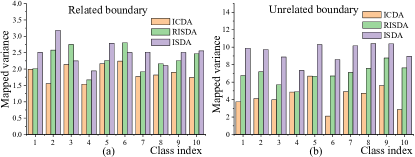
Figure 8: The variation of mapped variances towards normal vectors of boundaries related to (a) and unrelated to (b) the ground-truth category on standard CIFAR10 using ResNet-32.

Next, we demonstrate ICDA’s superiority. Compared with other methods, ${R}_{ICDA}$ can force models to simultaneously increase and decrease ${q}_{i,y_{i}}$ and ${q}_{i,c}$, respectively. Thus, sample margins, especially those of hard ones will be enlarged because the harder the sample, the larger the $\alpha_{i}$. Fig. 7 depicts the margin distributions of ISDA, RISDA, and ICDA, demonstrating that ICDA has fewer samples predicted correctly with small margins compared to the other two methods. In addition, the term $\Delta\boldsymbol{w}_{c,y_{i}}\boldsymbol{\mu}_{c}$ in $R_{ICDA}$ increases the class-boundary distance for class $y_{i}$. Like LA, the term ${q}_{i,c}\delta_{c,{i}}$ more increases the class-wise margins of the tail categories, manifesting that ICDA can deal well with imbalanced classification. Furthermore, $\Delta\boldsymbol{w}_{c,y_{i}}(\Sigma_{y_{i}}\!+\!\sum_{j=1,j\neq y_{i}}^{C}\hat{\alpha}_{i,j}\Sigma_{{j}})\Delta\boldsymbol{w}_{c,y_{i}}^{\top}$is the mapped variance of all relevant classes to the normal vector of the boundary between classes $y_{i}$ and $c$. Since this term is sample-wise, our punishment on the mapped variances is more refined and accurate than the class-wise approaches, enforcing better intra-class compactness. Fig. 6(c) reveals that although $C_{2}$ and $C_{1}$ are more confusing, the samples in the red circle are the most correlated with $C_{3}$ and cannot be taken seriously by the class-wise approaches. From Fig. 8, ICDA decreases the mapped variances on not only the boundaries related to the ground-truth category but also the unrelated ones to a higher degree. The $\beta$ and ${\lambda}$ parameters in $R_{ICDA}$ can control the effect of each component.

VII Experiments

We empirically validate ICDA on several typical learning scenarios (i.e., biased datasets including both imbalanced and noisy data, subpopulation shifts datasets, generalized long-tailed datasets, and standard datasets) regarding performance and efficiency. Both image and text datasets are evaluated. For a fair comparison, Meta-ICDA is only compared when the competitor method utilizes meta-learning. We also visualize the augmented samples in the original input space and the attention of the trained model on several images. Finally, we conduct ablation studies and sensitivity tests. Regarding the hyperparameter settings in ICDA, $\lambda^{0}$ is selected in $\{0.1,0.25,0.5,0.75,1\}$, and $\beta$ is set to $0.1$ in all subsections.

TABLE II: Top-1 accuracy on long-tailed CIFAR datasets. Bold and underlined numbers are the best and second-best results.

Dataset	CIFAR10		CIFAR100
Imbalance ratio	100:1	10:1	100:1	10:1
Class-balanced CE [31]	72.68%	86.90%	38.77%	57.57%
Class-balanced Focal [31]	74.57%	87.48%	39.60%	57.99%
LDAM [23]	73.55%	87.32%	40.60%	57.29%
LDAM-DRW [23]	78.12%	88.37%	42.89%	58.78%
LA [24]	77.67%	88.93%	43.89%	58.34%
LPL [32]	77.95%	89.41%	44.25%	60.97%
ALA [33]	77.65%	88.32%	43.67%	58.92%
De-confound-TDE [34]	80.60%	88.50%	44.10%	59.60%
MixUp [35]	73.10%	87.10%	39.50%	58.00%
ISDA [7]	72.55%	87.02%	37.40%	55.51%
RISDA [9]	79.89%	89.36%	50.16%	62.38%
ICDA (Ours)	81.69%	90.62%	50.18%	63.45%
Meta-Weight-Net [36]	73.57%	87.55%	41.61%	58.91%
MetaSAug [8]	80.54%	89.44%	46.87%	61.73%
Meta-ICDA (Ours)	82.47%	91.13%	50.96%	63.97%

TABLE III: Additional training time increased by ICDA loss compared with CE loss.

Networks	Params	Additional cost
		CIFAR10	CIFAR100
ResNet-32	0.5M	6.9%	6.9%
ResNet-56	0.9M	7.1%	7.2%
ResNet-110	1.7M	6.8%	6.7%
DenseNet-BC-121	8M	5.6%	5.3%
DenseNet-BC-265	33.3M	5.3%	5.1%
Wide ResNet-16-8	11.0M	6.8%	7.0%
Wide ResNet-28-10	36.5M	6.7%	6.8%

VII-A Experiments on Biased Datasets

Experiments on Long-tailed CIFAR Datasets

Settings. Long-tailed CIFAR is the long-tailed version of the CIFAR [37] data. Following Cui et al. [31], we discard some training samples to construct imbalanced datasets. Two training sets with imbalance ratios of 100:1 and 10:1 are built. We train ResNet-32 [38] with an initial learning rate of $0.1$ and the standard SGD with the momentum of $0.9$ and a weight decay of $5\!\times\!10^{-4}$. The learning rate is decayed by $0.1$ at the 120-th and 160-th epochs. As for the meta-learning-based algorithms, the initial learning rate is $0.1$ and it is decayed by $0.01$ at the 160-th and 180-th epochs following MetaSAug [8]. We randomly select ten images per class from training data to construct metadata.

Several classical and advanced robust loss functions and data augmentation approaches that are mainly designed for long-tailed classifications are compared, including Class-balanced CE loss [31], Class-balanced Focal loss, LDAM [23], LDAM-DRW [23], ISDA [7], LA [24], ALA [33], LPL [32], MixUp [35], and RISDA [9]. Besides, De-confound-TDE [34], which uses causal intervention in training and counterfactual reasoning in inference, is also involved in our comparison. Two meta-learning-based methods including Meta-Weight-Net [36] and MetaSAug [8] are also compared.

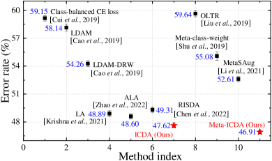
Figure 9: Top-1 error rate on ImageNet-LT.

Results. Table II reports the results on long-tailed CIFAR data, which are divided into two groups according to the usage of meta-learning. The results reveal that ICDA significantly outperforms other reweighting, solely logit adjustment, and implicit semantic augmentation methods, demonstrating that our sample-wise counterfactual augmentation strategy deals well with long-tailed classification. Although ICDA and RISDA achieve comparable performance on CIFAR100 with an imbalance ratio of 100:1, ICDA outperforms RISDA in other cases. Additionally, ICDA consistently surpasses De-confound-TDE, which uses causal intervention in training and counterfactual reasoning in inference. Our Meta-ICDA achieves state-of-the-art performance compared to all approaches.

To evaluate efficiency, we record the additional training time for ICDA and compare it against CE and ISDA. Table III reports the additional training time introduced by ICDA loss compared with CE loss on various backbones. The additional time introduced by ISDA loss compared with CE loss can be seen in the ISDA paper [7]. The results reveal that only a little time is increased by ICDA loss, and the values of training time for ICDA and ISDA are nearly equivalent.

Experiments on Long-tailed ImageNet Dataset

Settings. ImageNet [39] is a benchmark visual recognition dataset, which contains 1,281,167 training images and 50,000 validation images. Liu et al. [40] built the long-tailed version of ImageNet, which is denoted as ImageNet-LT. After discarding some training samples, ImageNet-LT remains 115,846 training examples in 1,000 classes. The imbalance ratio of ImageNet-LT is 256:1. Following MetaSAug [8], we adopt the original validation set to test methods. Ten images per category which are selected from the balanced validation set compiled by Liu et al. [40] are utilized to construct our metadata. ResNet-50 [38] is used as the backbone network. The learning rate is decayed by $0.1$ at the 60-th and the 80-th epochs. The batch size is set to $64$. Only the last fully connected layer is finetuned for training efficiency.

TABLE IV: Top-1 accuracy on CIFAR datasets with flip noise.

Dataset	CIFAR10		CIFAR100
Flip noise ratio	20%	40%	20%	40%
CE loss	76.83%	70.77%	50.86%	43.01%
$L_{DMI}$ [41]	86.70%	84.00%	62.26%	57.23%
JoCoR [42]	90.78%	83.67%	65.21%	45.44%
D2L [43]	87.66%	83.89%	63.48%	51.83%
Co-teaching [44]	82.83%	75.41%	54.13%	44.85%
APL [45]	87.23%	80.08%	59.37%	52.98%
ISDA [7]	88.90%	86.14%	64.36%	59.48%
RISDA [9]	85.48%	81.12%	61.81%	54.60%
ICDA (Ours)	91.81%	88.76%	66.85%	61.57%
GLC [46]	89.68%	88.92%	63.07%	62.22%
MentorNet [47]	86.36%	81.76%	61.97%	52.66%
L2RW [48]	87.86%	85.66%	57.47%	50.98%
Meta-Weight-Net [36]	90.33%	87.54%	64.22%	58.64%
MetaSAug [8]	90.42%	87.73%	66.47%	61.43%
Meta-ICDA (Ours)	92.46%	90.21%	67.54%	63.26%

TABLE V: Top-1 accuracy on CIFAR datasets with uniform noise.

Dataset	CIFAR10		CIFAR100
Uniform noise ratio	40%	60%	40%	60%
CE loss	68.07%	53.12%	51.11%	30.92%
$L_{DMI}$ [41]	85.90%	79.60%	63.16%	55.37%
JoCoR [42]	89.15%	64.54%	65.45%	44.43%
D2L [43]	85.60%	68.02%	52.10%	41.11%
Co-teaching [44]	74.81%	73.06%	46.20%	35.67%
APL [45]	86.49%	79.22%	57.84%	49.13%
ISDA [7]	88.11%	83.12%	65.15%	58.19%
RISDA [9]	83.25%	76.31%	54.09%	45.57%
ICDA (Ours)	90.23%	84.91%	67.24%	60.26%
GLC [46]	88.28%	83.49%	61.31%	50.81%
MentorNet [47]	87.33%	82.80%	61.39%	36.87%
L2RW [48]	86.92%	82.24%	60.79%	48.15%
Meta-Weight-Net [36]	89.27%	84.07%	67.73%	58.75%
MetaSAug [8]	89.32%	84.65%	66.50%	59.84%
Meta-ICDA (Ours)	91.14%	85.86%	68.92%	61.80%

Methods designed for long-tailed classification including Class-balanced CE loss [31], OLTR [40], LDAM [23], LDAM-DRW [23], LA [24], ALA [33], RISDA [9], Meta-class-weight [36], and MetaSAug [8] are compared.

Results. Fig. 9 highlights that ICDA achieves good performance among the robust losses. Meta-ICDA significantly outperforms all competitor methods, including the meta semantic augmentation approach, proving that our proposed approach is more effective on long-tailed data.

Experiments on Noisy CIFAR Datasets

Settings. Following Shu et al [36], two settings of corrupted labels are adopted, namely, uniform and pair-flip noise labels; 1,000 images with clean labels in the validation set are selected as the metadata. Wide ResNet-28-10 (WRN-28-10) [49] and ResNet-32 [38] are adopted as the classifiers for the uniform and pair-flip noises, respectively. The initial learning rate and batch size are set to $0.1$ and $128$, respectively. For ResNet, standard SGD with the momentum of $0.9$ and a weight decay of $1\!\times\!10^{-4}$ is utilized. For Wide ResNet, standard SGD with the momentum of $0.9$ and a weight decay of $5\!\times\!10^{-4}$ is utilized. As for the meta-learning-based algorithms, the initial learning rate is $0.1$ and it is decayed by $0.01$ at the 160-th and 180-th epochs following MetaSAug [8].

TABLE VI: Average and worst-group accuracy on subpopulation shifts datasets.

Dataset	CelebA		CMNIST		Waterbirds		CivilComments
Method	Avg.	Worst	Avg.	Worst	Avg.	Worst	Avg.	Worst
UW [50]	92.9%	83.3%	72.2%	66.0%	95.1%	88.0%	89.8%	69.2%
IRM [51]	94.0%	77.8%	72.1%	70.3%	87.5%	75.6%	88.8%	66.3%
IB-IRM [52]	93.6%	85.0%	72.2%	70.7%	88.5%	76.5%	89.1%	65.3%
V-REx [53]	92.2%	86.7%	71.7%	70.2%	88.0%	73.6%	90.2%	64.9%
CORAL [54]	93.8%	76.9%	71.8%	69.5%	90.3%	79.8%	88.7%	65.6%
GroupDRO [55]	92.1%	87.2%	72.3%	68.6%	91.8%	90.6%	89.9%	70.0%
DomainMix [56]	93.4%	65.6%	51.4%	48.0%	76.4%	53.0%	90.9%	63.6%
Fish [57]	93.1%	61.2%	46.9%	35.6%	85.6%	64.0%	89.8%	71.1%
LISA [50]	92.4%	89.3%	74.0%	73.3%	91.8%	89.2%	89.2%	72.6%
ICDA (Ours)	93.3%	90.7%	76.1%	75.3%	92.9%	90.7%	91.1%	73.5%

TABLE VII: Top-1 accuracy and precision of CLT, GLT, and ALT protocols on ImageNet-GLT.

Protocol	CLT		GLT		ALT
Method	Acc.	Prec.	Acc.	Prec.	Acc.	Prec.
CE loss	42.52%	47.92%	34.75%	40.65%	41.73%	41.74%
cRT [58]	45.92%	45.34%	37.57%	37.51%	41.59%	41.43%
LWS [58]	46.43%	45.90%	37.94%	38.01%	41.70%	41.71%
De-confound-TDE [34]	45.70%	44.48%	37.56%	37.00%	41.40%	42.36%
BLSoftmax [59]	45.79%	46.27%	37.09%	38.08%	41.32%	41.37%
LA [24]	46.53%	45.56%	37.80%	37.56%	41.73%	41.74%
BBN [60]	46.46%	49.86%	37.91%	41.77%	43.26%	43.86%
LDAM [23]	46.74%	46.86%	38.54%	39.08%	42.66%	41.80%
IFL [27]	45.97%	52.06%	37.96%	44.47%	45.89%	46.42%
MixUp [35]	38.81%	45.41%	31.55%	37.44%	42.11%	42.42%
RandAug [61]	46.40%	52.13%	38.24%	44.74%	46.29%	46.32%
ISDA [7]	47.66%	51.98%	39.44%	44.26%	47.62%	47.46%
RISDA [9]	49.31%	50.64%	38.45%	42.77%	47.33%	46.33%
ICDA (Ours)	52.11%	55.05%	42.73%	47.49%	50.52%	49.68%
MetaSAug [8]	50.53%	55.21%	41.27%	47.38%	49.12%	48.56%
Meta-ICDA (Ours)	52.76%	56.71%	44.15%	49.32%	51.74%	51.43%

Several robust loss functions including Information-theoretic Loss ($L_{DMI}$) [41], JoCoR [42], Co-teaching [44], D2L [43], and APL [45] are compared. The meta-learning-based methods, including MentorNet [47], L2RW [48], GLC [46], and Meta-Weight-Net [36] are also involved in comparison. We also compared our proposed ICDA with three implicit data augmentation methods, including ISDA [7], RISDA [9], and MetaSAug [8].

There is a small variation of our method on noisy occasions. As we do not wish the model to pay too much attention to noisy samples, we add a compensation term to the logit of their ground-truth classes after flipping, which is the opposite of the original $\alpha_{i}$. Therefore, on noisy occasions, the value of $\alpha_{i}$ is:

$$\alpha_{i}=\begin{cases}\frac{1-\cos\theta_{i,y_{i}}}{2}\quad\text{if}~{}\frac{1-\cos\theta_{i,y_{i}}}{2}<\tau,\\ \frac{\cos\theta_{i,y_{i}}-1}{2}\quad\text{else},\end{cases}$$ (19)

where $\tau$ is a hyperparameter, set to $0.9$ in our experiments.

Results. Table IV and Table V report the results of CIFAR data with flip and uniform noise, respectively. ICDA notably surpasses all competitor approaches including robust loss functions and the class-level implicit data augmentation approaches. Besides, Meta-ICDA achieves state-of-the-art performance compared with other meta-learning-based manners, manifesting that our proposed method can effectively improve the generalization and robustness of models on noisy data.

VII-B Experiments on Subpopulation Shifts Datasets

Settings. Four subpopulation shifts datasets are evaluated, including CMNIST, Waterbirds [55], CelebA [20], and CivilComments [62], in which the domain information is highly spuriously correlated with the labels. Detailed descriptions of the datasets are shown in Appendix E. In the subsequent trials, ResNet-50 is utilized as the backbone network for the first three image datasets, while DistilBert [63] is adopted for the text set CivilComments. The initial learning rates for CMNIST and Waterbirds are $1\times 10^{-3}$, while those for CelebA and Civilcomments are $1\times 10^{-4}$ and $1\times 10^{-5}$, respectively. The values of weight decay are $1\times 10^{-4}$ for CMNIST, Waterbirds, and CelebA, and $0$ for CivilComments. The values of batch size for CMNIST, Waterbirds, and CelebA are $16$, and that for Civilcomments is $8$. For the three image classification datasets, SGD optimizer is utilized, while Adam is utilized for Civilcomments.

Robust methods, including IRM [51], IB-IRM [52], V-REx [53], CORAL [54], GroupDRO [55], DomainMix [56], Fish [57], and LISA [50], are compared. Upweighting (UW) is suitable for subpopulation shifts, so we also use it for comparison. We only compare ICDA with other methods for fair comparisons as all these approaches do not rely on meta-learning. Following Yao et al. [50], the worst-group accuracy is used to compare the performance of all methods.

TABLE VIII: Top-1 accuracy and precision of CLT, GLT, and ALT protocols on MSCOCO-GLT.

Protocol	CLT		GLT		ALT
Method	Acc.	Prec.	Acc.	Prec.	Acc.	Prec.
CE loss	72.34%	76.61%	63.79%	70.52%	50.17%	50.94%
cRT [58]	73.64%	75.84%	64.69%	68.33%	49.97%	50.37%
LWS [58]	72.60%	75.66%	63.60%	68.81%	50.14%	50.61%
De-confound-TDE [34]	73.79%	74.90%	66.07%	68.20%	50.76%	51.68%
BLSoftmax [59]	72.64%	75.25%	64.07%	68.59%	49.72%	50.65%
LA [24]	75.50%	76.88%	66.17%	68.35%	50.17%	50.94%
BBN [60]	73.69%	77.35%	64.48%	70.20%	51.83%	51.77%
LDAM [23]	75.57%	77.70%	67.26%	70.70%	55.52%	56.21%
IFL [27]	74.31%	78.90%	65.31%	72.24%	52.86%	53.49%
MixUp [35]	74.22%	78.61%	64.45%	71.13%	48.90%	49.53%
RandAug [61]	76.81%	79.88%	67.71%	72.73%	53.69%	54.71%
ISDA [7]	77.32%	79.23%	67.57%	72.89%	54.43%	54.62%
RISDA [9]	76.34%	79.27%	66.85%	72.66%	54.58%	53.98%
ICDA (Ours)	78.82%	81.33%	68.78%	74.29%	56.48%	57.81%

Results. Table VI reports the results of the four subpopulation shifts datasets. The performance of methods that learn invariant predictors with explicit regularizers, e.g., IRM, IB-IRM, and V-REx, is not consistent across datasets. For example, V-REx outperforms IRM on CelebA, but it fails to achieve better performance than IRM on CMNIST, Waterbirds, and CivilComments. Opposing, ICDA consistently achieves an appealing performance on all datasets, demonstrating ICDA’s effectiveness in breaking spurious correlations and achieving invariant feature learning. Although ICDA and GroupDRO achieve similar performance on Waterbirds, ICDA far exceeds GroupDRO on the other three datasets.

TABLE IX: Top-1 error rate on standard CIFAR datasets.

Backbone	ResNet-110		WRN-28-10
Dataset	CIFAR10	CIFAR100	CIFAR10	CIFAR100
Large Margin [64]	6.46%	28.00%	3.69%	18.48%
Disturb Label [65]	6.61%	28.46%	3.91%	18.56%
Focal loss [66]	6.68%	28.28%	3.62%	18.22%
Center loss [67]	6.38%	27.85%	3.76%	18.50%
Lq loss [68]	6.69%	28.78%	3.78%	18.43%
WGAN [69]	6.63%	-	3.81%	-
CGAN [70]	6.56%	28.25%	3.84%	18.79%
ACGAN [71]	6.32%	28.48%	3.81%	18.54%
infoGAN [72]	6.59%	27.64%	3.81%	18.44%
ISDA [7]	5.98%	26.35%	3.58%	17.98%
RISDA[9]	6.47%	28.42%	3.79%	18.46%
ICDA (Ours)	4.89%	25.21%	3.01%	17.03%

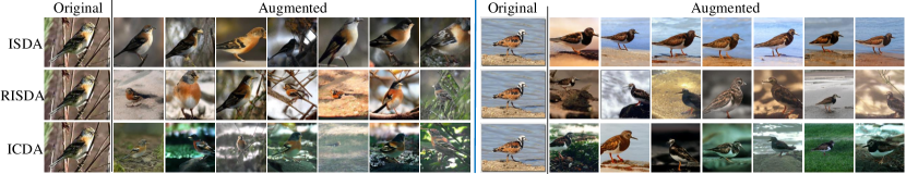
Figure 10: Visualization of images augmented by ISDA, RISDA, and ICDA.

VII-C Experiments on Generalized Long-tailed Datasets

Settings. Tang et al. [27] proposed a novel learning problem, namely, generalized long-tailed classification, in which two new benchmarks, including MSCOCO-GLT and ImageNet-GLT, were proposed. Each benchmark has three protocols, i.e., CLT, ALT, and GLT, in which class distribution, attribute distribution, and both class and attribute distributions are changed from training to testing, respectively. More details of the two benchmarks can be seen in [27]. The training and testing configurations follow those in the IFL [27] paper. ResNeXt-50 [73] is used as the backbone network for all methods except for BBN [60]. Both Top-1 accuracy and precision are presented. All models are trained with a batch size of $256$ and an initial learning rate of $0.1$. SGD optimizer is utilized with a weight decay of $5\times 10^{-4}$ and the momentum of $0.9$. Here, Meta-ICDA was exclusively evaluated on the ImageNet-GLT benchmark. To collect the attribute-wise balanced metadata, images from each class in a balanced validation set compiled by Liu et al. [40] were clustered into 6 groups by KMeans using a pre-trained ResNet-50 model following Tang et al. [27]. From each group and class, 10 images were sampled to construct the metadata.

As for the compared methods, we studied two-stage re-sampling methods, including cRT [58] and LWS [58], posthoc distribution adjustment methods including De-confound-TDE [34] and LA [24], multi-branch models with diverse sampling strategies like BBN [60], invariant feature learning methods like IFL [27], and reweighting loss functions like BLSoftmax [59] and LDAM [23]. We also compare some data augmentation methods, including MixUp [35], RandAug [61], ISDA [7], RISDA [9], and MetaSAug [8].

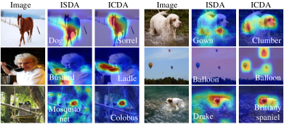
Figure 11: Visualization of the regions that the model used for making predictions. Blue and red imply that the region is indecisive and very discriminative, respectively. White texts are the predicted labels.

Results. Table VII and Table VIII report the results of the three protocols for ImageNet-GLT and MSCOCO-GLT, respectively, some of which are from the IFL [27] paper. ICDA notably improves model performance in all three protocols, demonstrating that it can well break the spurious associations caused by imbalanced attribute and class distributions, while the majority of previous LT algorithms using rebalancing strategies fail to improve the robustness against the attribute-wise bias. Additionally, we found that augmentation methods generally perform better than other long-tailed transfer learning approaches on GLT protocols.

VII-D Experiments on Standard CIFAR Datasets

Settings. To verify that ICDA has a good augmentation effect, it is compared with a number of advanced methods ranging from robust loss functions (i.e., Large Margin [64], Dsitrub Label [65], Focal loss [66], Center loss [67], and Lq loss [68]) to explicit (i.e., WGAN [69], CGAN [70], ACGAN [71], and infoGAN [72]) and implicit (i.e., ISDA [7] and RISDA [9]) augmentation methods on standard CIFAR data.

Regarding the hyperparameter settings, the initial learning rate and the batch size are set to $0.1$ and $128$, respectively. For ResNet, standard SGD with the momentum of $0.9$ and a weight decay of $1\!\times\!10^{-4}$ is utilized. For Wide ResNet, standard SGD with the momentum of $0.9$ and a weight decay of $5\!\times\!10^{-4}$ is utilized. The learning rate is decayed by $0.1$ at the 120-th and 160-th epochs.

Results. The results of ResNet-110 and WRN-28-10 are reported in Table IX. ICDA achieves the best performance compared with the other explicit and implicit augmentation approaches. Moreover, GAN-based methods perform poorly on CIFAR100 due to a limited training size. Additionally, these methods impose excess calculations and decrease training efficiency. Although ISDA affords lower error and is more efficient than GAN-based schemes, it can not surpass ICDA as it assists the models to break spurious correlations among the classes.

VII-E Visualization Results

Following ISDA’s visualization manner, we map the augmented features back into the pixel space. The corresponding results are presented in Fig. 10, highlighting that ICDA can generate more diverse and meaningful counterfactual images and notably alter the non-intrinsic attributes, e.g., scene contexts and viewpoints, compared with ISDA and RISDA.

Figure 12: Results of ablation studies on standard and imbalanced CIFAR data.

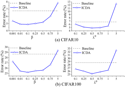
Figure 13: Results of the sensitivity tests on standard CIFAR datasets.

Additionally, Grad-CAM [74] is utilized to visualize the regions that models used for making predictions. Fig. 11 manifests that ISDA focuses on the background or other nuisances for false predictions, while ICDA focuses tightly on the causal regions corresponding to the object, assisting models to make correct classifications. For example, for the image of “Brittany spaniel”, ISDA utilizes spurious context “Water”, so its prediction is “Drake”, while the model trained with ICDA attends more to the dog, contributing to a correct prediction. Therefore, in addition to performance gains, the ICDA predictions are made for the right reasons. More visualization results are shown in Appendix F.

VII-F Ablation and Sensitivity Studies

To get a better understanding of the effect of varying components, we evaluate the following three settings of ICDA. Setting I: Without the covariance matrices and feature means of the other categories, i.e., $\alpha_{i,c}=0$. Setting II: Without the class-level logit perturbation term, i.e., removing $\delta_{c,i}$. Setting III: Without the sample-level logit perturbation term, i.e., removing $\beta\alpha_{i}$. Since the proportion of each class is the same on standard data, we only evaluate Settings I and III on the standard data. The ablation results are presented in Fig. 12, revealing that all three components are crucial and necessary for imbalanced data. Additionally, the statistics information of the other classes and the sample-level perturbation term are critical for standard data. Without each of them, the performance of ICDA will be weakened.

To study how the hyperparameters in ICDA (i.e., $\lambda^{0}$ and $\beta$) affect our method’s performance, several sensitivity tests are conducted, where ResNet-110 is used as the backbone network. The corresponding results on standard CIFAR data are shown in Fig. 13, revealing that ICDA achieves superior performance for $0.01\leq\beta\leq 0.5$ and $0.25\leq\lambda^{0}\leq 1$. When $\beta$ and $\lambda^{0}$ are too large, the model is easier to overfit and underfit, respectively. Empirically, we recommend $\beta=0.1$ and $\lambda^{0}=0.5$ for a naive implementation or a starting point of hyperparameter searching.

VIII Conclusion

This study proposes a sample-wise implicit counterfactual data augmentation (ICDA) method to break spurious correlations and make stable predictions. Our method can be formulated as a novel robust loss, easily adopted by any classifier, and is considerably more efficient than explicit augmentation approaches. Two manners, including direct quantification and meta-learning, are introduced to learn the key parameters in the robust loss. Furthermore, the regularization analysis demonstrates that ICDA improves intra-class compactness, class and sample-wise margins, and class-boundary distances. Extensive experimental comparison and visualization results on several typical learning scenarios demonstrate the proposed method’s effectiveness and efficiency.

Appendix A Derivation of Surrogate Loss

The networks can be trained by minimizing the following CE loss for the augmented sample features:

where $\tilde{M}=\sum_{i=1}^{N}\sum_{c=1,c\neq y_{i}}^{C}\tilde{M}_{i,c}$ and $f_{y_{i}}(\boldsymbol{h}_{i,c}^{k})=\boldsymbol{w}_{y_{i}}^{\top}\boldsymbol{h}_{i,c}^{k}+{b}_{y_{i}}$. Obviously, the naive implementation is computationally inefficient when $M$ in $\tilde{M}_{i,c}$ is large.

We consider the case that $M$ grows to infinity and find that an easy-to-compute upper bound can be derived for the expected loss, which leads to a highly efficient implementation. We have

where $\Delta\boldsymbol{w}_{j,y_{i}}=\boldsymbol{w}_{j}^{\top}-\boldsymbol{w}_{y_{i}}^{\top}$ and $\Delta{b}_{j,y_{i}}={b}_{j}-{b}_{y_{i}}$. $P_{j,{i},c}=\Delta\boldsymbol{w}_{j,y_{i}}(\Sigma_{y_{i}}+\alpha_{i,c}\Sigma_{{c}})\Delta\boldsymbol{w}_{j,y_{i}}^{\top}$ and $Q_{j,{i},c}=\Delta\boldsymbol{w}_{j,y_{i}}\alpha_{i,c}\boldsymbol{\mu}_{c}$. In addition, $\tilde{N}_{i,c}={\alpha_{i,c}}/{\pi_{y_{i}}}$ and $\tilde{N}=\sum_{i=1}^{N}\sum_{c=1,c\neq y_{i}}^{C}\tilde{N}_{i,c}$. The fourth step in Eq. (21) follows from the Jensen’s inequality $\mathrm{E}[\log X]\leq\log\mathrm{E}[X]$ as function $\log(\cdot)$ is concave. The fifth step in Eq. (21) utilizes the moment-generating function, which is

$$\mathrm{E}\left[\exp({tX})\right]=\exp({t\mu+\frac{1}{2}\sigma^{2}t^{2}}),\quad X\sim\mathcal{N}(\mu,\sigma^{2}).$$ (22)

We know that $\Delta\boldsymbol{w}_{j,y_{i}}\boldsymbol{h}_{i,c}+\Delta{b}_{j,y_{i}}$ is a Gaussian random variable, i.e.,

Thus, we have

From the above formula, $\alpha_{i,c}$ can be viewed as a weight for the loss of sample $\boldsymbol{x}_{i}$ to class $c$. Although weighting is direct, it has minimal effect in separable settings: solutions that achieve zero training loss will necessarily remain optimal even under weighting [24]. Intuitively, one would like instead to increase the margins of samples that are most affected by the spurious correlation between $\boldsymbol{x}_{i}$ and class $c$ (with large $\alpha_{i,c}$). Thus, we add a sample-wise margin to the above loss, which is

where the sample-wise margin is $\Delta_{i,c}=\beta\alpha_{i,c}$ and $\beta$ is a hyperparameter. In this way, we have the following loss

$\ell_{i,c}$ in Eq. (26) can be written as $CE(f(\boldsymbol{h}_{i})+[\frac{\lambda}{2}P_{1,{i},c}+\lambda Q_{1,{i},c},\cdots,-\beta\alpha_{i,c},\cdots,\frac{\lambda}{2}P_{C,{i},c}+\lambda Q_{C,{i},c}])$, where $CE$ refers to the CE loss. With the first-order Taylor expansion, we yield

Using Taylor expansion again, our surrogate loss is

where $P_{j,i}\!=\!\Delta\boldsymbol{w}_{j,y_{i}}(\Sigma_{y_{i}}\!+\!\sum_{c=1,c\neq y_{i}}^{C}\hat{\alpha}_{i,c}\Sigma_{{c}})\Delta\boldsymbol{w}_{j,y_{i}}^{\top}$, $Q_{j,i}=\Delta\boldsymbol{w}_{j,y_{i}}\sum_{c=1,c\neq y_{i}}^{C}\hat{\alpha}_{i,c}\boldsymbol{\mu}_{c}$, and $\hat{\alpha}_{i,c}={{\alpha}_{i,c}}/{(C-1)}$. Denote $\alpha_{i}=\sum_{c=1,c\neq y_{i}}^{C}{\hat{\alpha}}_{i,c}$. Then, our loss function becomes

As stated in Section IV.B, we leveraged two following modifications to achieve a more effective loss: (1) Inspired by LA [24], the class-wise weight $1/\pi_{y_{i}}$ is replaced by a perturbation term on logits. (2) We only retain the term $\Delta\boldsymbol{w}_{{j},y_{i}}\hat{\alpha}_{i,j}\boldsymbol{\mu}_{j}$ in $Q_{j,{i}}$. Accordingly, our final optimized ICDA loss becomes

where $\delta_{j,i}=\log({\pi_{j}}/{\pi_{{y_{i}}}})$.

Appendix B Calculation of $\boldsymbol{\mu}$ and $\Sigma$

The feature means $\boldsymbol{\mu}$ and covariance matrices $\Sigma$ are calculated online by aggregating statistics from all mini-batches, following ISDA [7]. During the training process using $\overline{\mathcal{L}}_{s}$, the feature means are estimated by:

$$\boldsymbol{\mu}_{c}^{(t)}=\frac{n_{c}^{(t-1)}\boldsymbol{\mu}_{c}^{(t-1)}+m_{c}^{(t)}{\boldsymbol{\mu}_{c}^{\prime}}^{(t)}}{n_{c}^{(t-1)}+m_{c}^{(t)}},$$ (31)

where ${\boldsymbol{\mu}_{c}}^{(t)}$ and ${\boldsymbol{\mu}_{c}^{\prime}}^{(t)}$ are the feature mean estimates of $c$-th class at the $t$-th step and in the $t$-th mini-batch, respectively. $n_{c}^{(t-1)}$ and $m_{c}^{(t)}$ denote the total number of training samples belonging to the $c$-th class in all $t-1$ mini-batches and the number of training samples belonging to $c$-th class only in $t$-th mini-batch. The covariance matrices are estimated by:

$$\Sigma_{c}^{(t)} =\frac{n_{c}^{(t-1)}\Sigma_{c}^{(t-1)}+m_{c}^{(t)}\Sigma_{c}^{\prime(t)}}{n_{c}^{(t-1)}+m_{c}^{(t)}}$$ (32)

$$+\frac{n_{c}^{(t-1)}m_{c}^{(t)}\left(\boldsymbol{\mu}_{c}^{(t-1)}-\boldsymbol{\mu}_{c}^{\prime(t)}\right)\left(\boldsymbol{\mu}_{c}^{(t-1)}-\boldsymbol{\mu}_{c}^{\prime(t)}\right)^{\top}}{\left(n_{c}^{(t-1)}+m_{c}^{(t)}\right)^{2}},$$

where ${\Sigma_{c}}^{(t)}$ and ${{\Sigma}_{c}^{\prime}}^{(t)}$ are the covariance matrix estimates of the $c$-th class at the $t$-th step and in the $t$-th mini-batch, respectively. Additionally, $n_{c}^{(t)}=n_{c}^{(t-1)}+m_{c}^{(t)}$.

Appendix C Extracted Training Characteristics

In the framework of Meta-ICDA, the augmentation strengths of samples are determined by the training characteristics of samples. Thus, ten training characteristics (${\zeta}_{i,1},{\zeta}_{i,2},\cdots,{\zeta}_{i,10}$) reflecting the samples’ training behavior are extracted from the classifier and input into the strength generation network, in which the first six characteristics follow those in the CAAT paper [75]. The characteristics are detailed as follows:

(1) Loss (${\zeta}_{i,1}$) is the most commonly utilized factor to reflect a sample’s training behavior [36]. Typically, the higher the loss, the more challenging the sample is considered to be.

(2) Margin (${\zeta}_{i,2}$), which measures the learning difficulty of samples, refers to the distance from the sample to the classification boundary [76]. To compute it, the following formula is used:

$${\zeta}_{i,2}=\boldsymbol{q}_{i,y_{i}}-\text{max}_{c\neq{y_{i}}}(\boldsymbol{q}_{i,c}),$$ (33)

where $\boldsymbol{q}_{i,c}$ refers to the predicted probability of sample $\boldsymbol{x}_{i}$ for class $c$.

(3)The norm of the loss gradient (${\zeta}_{i,3}$) of $\boldsymbol{q}_{i}$ also reflects the learning difficulty of samples [40]. In general, samples with large norms of the gradient are hard ones. Since the CE loss is adopted, it can be calculated by:

$${\zeta}_{i,3}=||\boldsymbol{y}_{i}-\boldsymbol{q}_{i}||_{2},$$ (34)

where $\boldsymbol{y}_{i}$ is the one-hot label vector of sample $\boldsymbol{x}_{i}$.

(4) Information entropy (${\zeta}_{i,4}$) of $\boldsymbol{q}_{i}$ can be used to quantify the uncertainty of samples [77], and is calculated as:

$${\zeta}_{i,4}=-\sum_{c=1}^{C}\boldsymbol{q}_{i,c}\log_{2}(\boldsymbol{q}_{i,c}).$$ (35)

(5) Class proportion (${\zeta}_{i,5}$) is always utilized to address long-tailed learning occasions [31], which is calculated as:

$${{\zeta}_{i,5}}=N_{{y}_{i}}/N,$$ (36)

where $N_{{y}_{i}}$ and $N$ denote the sample cardinality in class ${y}_{i}$ and in the entire training set, respectively.

(6) Average loss of each category (${\zeta}_{i,6}$) reflects the average learning difficulty of each category, which is

$${{\zeta}_{i,6}}=\bar{\ell}_{{y}_{{i}}},$$ (37)

where $\bar{\ell}_{{y}_{i}}$ is the average loss of samples in class ${y}_{i}$.

(7) Relative loss (${\zeta}_{i,7}$) is the difference between the loss of $\boldsymbol{x}_{i}$ and the average loss of category $y_{i}$:

$${\zeta}_{i,7}=\ell_{i}-\bar{\ell}_{{y}_{i}}.$$ (38)

(8) Relative margin (${\zeta}_{i,8}$) is the difference between the margin of $\boldsymbol{x}_{i}$ and the average margin of category $y_{i}$:

$${\zeta}_{i,8}=\zeta_{i,2}-\bar{\gamma}_{{y}_{i}},$$ (39)

where $\bar{\gamma}_{{y}_{i}}$ is the average margin of category $y_{i}$.

(9) The norm of the classifier weights (${\zeta}_{i,9}$) is verified to be effective in addressing long-tailed data [78], which is

$${\zeta}_{i,9}=||\boldsymbol{w}_{y_{i}}||_{2}^{2},$$ (40)

where $\boldsymbol{w}_{y_{i}}$ refers to the classifier weights of category ${y_{i}}$.

(10) The cosine value of the angle between the feature $\boldsymbol{h}_{i}$ and the weight vector $\boldsymbol{w}_{y_{i}}$ (${\zeta}_{i,10}$) [33] is given by:

$${\zeta}_{i,10}=\cos\theta_{i,y_{i}},$$ (41)

where $\cos\theta_{i,y_{i}}$ is derived through

$$f_{y_{i}}\left(\boldsymbol{h}_{i}\right) :={\boldsymbol{w}_{y_{i}}}^{\top}\boldsymbol{h}_{i}+{b}_{y_{i}}$$ (42)

$$:=\left\|\boldsymbol{w}_{y_{i}}\right\|\left\|\boldsymbol{h}_{i}\right\|\cos\theta_{i,y_{i}}\quad//\text{by omitting }\boldsymbol{b}_{y_{i}}$$

$$:=\left\|\boldsymbol{h}_{i}\right\|\cos\theta_{i,y_{i}}\quad//\text{// by weight normalization}$$

$$:=\cos\theta_{i,y_{i}}\quad//\text{by feature normalization}.$$

The ten training characteristics mentioned above are extracted from the classifier network and input into the strength generation network to generate the values of the augmentation strengths $\alpha_{i}$.

Appendix D Derivation of Regularization Terms

First, we obtain the logit perturbation terms of all four approaches (i.e., LA [24], ISDA [7], RISDA [9], and ICDA). Losses with logit adjustment can be summarized in the following form:

Then, the perturbation term for the ground-truth class is $\Delta{u}_{i,y_{i}}$ and that for other classes is $\Delta{u}_{i,j}$ ($j\neq y_{i}$). Our loss function for sample $\boldsymbol{x}_{i}$ is

where $P_{j,{i}}=\Delta\boldsymbol{w}_{j,y_{i}}(\Sigma_{y_{i}}+\sum_{c=1,c\neq y_{i}}^{C}\hat{\alpha}_{i,c}\Sigma_{c})\Delta\boldsymbol{w}_{j,y_{i}}^{\top}$. Therefore, the perturbation term for the ground-truth class is $\Delta{u}_{i,y_{i}}=-\beta\alpha_{i}$ and that for the negative classes is $\Delta{u}_{i,j}=\frac{{\lambda}}{2}P_{j,{i}}+{\lambda}\Delta\boldsymbol{w}_{j,y_{i}}\hat{\alpha}_{i,j}\boldsymbol{\mu}_{j}+\delta_{j,{i}}$.

ISDA [7] loss for sample $\boldsymbol{x}_{i}$ is

Therefore, $\Delta{u}_{i,y_{i}}=0$ and $\Delta{u}_{i,j}=\frac{\lambda}{2}\Delta\boldsymbol{w}_{j,y_{i}}\Sigma_{y_{i}}\Delta\boldsymbol{w}_{j,y_{i}}^{\top}$ in ISDA, in which $\lambda$ is a hyperparameter.

As for RISDA [9], its loss for $\boldsymbol{x}_{i}$ can be written as

Therefore, $\Delta{u}_{i,y_{i}}\!=\!0$ and $\Delta{u}_{i,j}={\alpha\Delta{\boldsymbol{w}_{j,y_{i}}}\sum_{c\neq{y_{i}}}^{C}{{\varepsilon_{y_{i},c}}{\boldsymbol{\mu}_{c}}}\!+\!\beta\Delta{\boldsymbol{w}_{j,y_{i}}}({\Sigma_{{y_{i}}}}\!+\!\sum_{c\neq{y_{i}}}^{C}{{\varepsilon_{y_{i},c}}}{\Sigma_{c}})\Delta\boldsymbol{w}_{j,y_{i}}^{\top}}$ in RISDA, in which $\alpha$ and $\beta$ are hyperparameters. $\varepsilon_{y_{i},c}$ measures the percentage of samples in category $y_{i}$ wrongly classified to category $c$.

The loss of sample $\boldsymbol{x}_{i}$ for LA [24] is

$$\ell_{LA}(\boldsymbol{u}_{i},y_{i})=-\log\frac{\exp({u}_{i,y_{i}}+\log\pi_{y_{i}})}{\sum_{j=1}^{C}\exp({u}_{i,j}+\log\pi_{j})}.$$ (47)

Thus, $\Delta{u}_{i,y_{i}}=\log\pi_{y_{i}}$ and $\Delta{u}_{i,j}=\log\pi_{j}$ in LA loss.

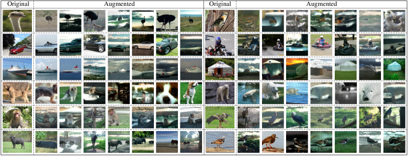
Figure 14: Extra visualization of the images augmented by our proposed ICDA. The first column represents the original images and the rest columns represent the augmented ones.

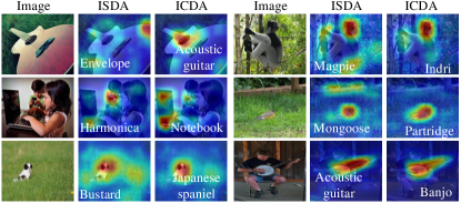
Figure 15: Extra visualization of the input regions that the model used for making predictions. ISDA makes false predictions of these images due to spurious correlations, while ICDA makes correct predictions based on the causal parts.

Then, we can derive the regularization terms of the four approaches on the basis of the Taylor expansion, which is

$$\ell(\boldsymbol{u}+\Delta\boldsymbol{u})\approx\ell(\boldsymbol{u})+(\frac{\partial\ell}{\partial\boldsymbol{u}})^{\top}\Delta\boldsymbol{u}=\ell(\boldsymbol{u})+(\boldsymbol{q}-\boldsymbol{y})^{\top}\Delta\boldsymbol{u},$$ (48)

where $\boldsymbol{q}=\text{softmax}(\boldsymbol{u})$. Then, the regularization term of the loss is $R=(\boldsymbol{q}-\boldsymbol{y})^{\top}\Delta\boldsymbol{u}$. Taking ICDA loss as an example, we can derive its regularization term according to Eq. (48), which is

Then, the regularization term for all samples in ICDA is

As $\beta\alpha_{i}$ in Eq. (50) is a constant which does not affect the optimization process, we omit it. Then, the regularizer of ICDA is

Following the same inference manner, we can derive the regularization terms for RISDA, ISDA, and LA losses. The regularization term of RISDA is

$${R}_{RISDA}=\sum_{i=1}^{N} \sum_{c\neq{y_{i}}}{{q}_{i,c}}[\alpha\Delta{\boldsymbol{w}_{c,{y_{i}}}}\sum_{j=1,j\neq{y_{i}}}^{C}{{\varepsilon_{y_{i},j}}{\boldsymbol{\mu}_{j}}}$$ (52)

$${+\beta\Delta{\boldsymbol{w}_{c,{y_{i}}}}({\Sigma_{y_{i}}}+\sum_{j=1,j\neq{y_{i}}}^{C}{{\varepsilon_{y_{i},j}}}{\Sigma_{j}})\Delta\boldsymbol{w}_{c,{y_{i}}}^{\top}}].$$

The regularization term of ISDA is

$${R}_{ISDA}=\sum_{i=1}^{N}\sum_{c\neq y_{i}}\frac{\lambda}{2}{q}_{i,c}\Delta\boldsymbol{w}_{c,{y_{i}}}\Sigma_{y_{i}}\Delta\boldsymbol{w}_{c,{y_{i}}}^{\top}.$$ (53)

The regularization term of LA is

$${R}_{LA}=\sum_{i=1}^{N}\sum_{c\neq y_{i}}{q}_{i,c}\delta_{c,i}.$$ (54)

Appendix E Details of Subpopulation Shifts Datasets

Following Yao et al. [50], the detailed information of the four subpopulation shifts datasets is detailed below.

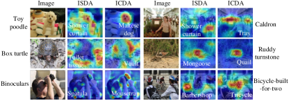
Figure 16: Visualization of the input regions that the model used for making predictions, in which both ISDA and ICDA make false predictions. White texts are the predictions of images. Black texts on the two sides are the ground-truth labels of the images.

CMNIST: MNIST digits are classified into 2 classes, where classes 0 and 1 include digits (0, 1, 2, 3, 4) and (5, 6, 7, 8, 9), respectively. The color of the digits is treated as a spurious attribute. Specifically, the proportion between red and green samples is 8:2 in class 0, while that is 2:8 in class 1. The proportion between green and red samples is 1:1 for both classes in the validation set. In the test set, the proportion between green and red samples is 1:9 in class 0, while the ratio is 9:1 in class 1. The numbers of samples in the training, validation, and test datasets are 30,000, 10,000, and 20,000, respectively. Following Arjovsky et al. [51], the labels were randomly flipped with a probability of 0.25.

Waterbirds [55]: This dataset aims to classify birds as “waterbird” or “landbird”. The spurious attribute is the scene context “water” or “land”. Waterbirds is a synthetic dataset in which each image is composed by pasting a bird image drawn from the CUB dataset [79] to a background sampled from the Places dataset [80]. The bird categories in CUB include landbirds and waterbirds. Two groups including (“land” background, “waterbird”) and (“water” background, “landbird”) are regarded as minority groups. There are 4,795 training samples of which 56 samples are “waterbirds on land” and 184 samples are “landbirds on water”. The remaining training samples include 3,498 samples from “landbirds on land”, and 1,057 samples from “waterbirds on water”.

CelebA [20]: CelebA includes a number of face images of celebrities. The classification labels are the hair colors of the celebrities including “blond” or “not blond.” The spurious attribute is gender, i.e., male or female. In CelebA, the minority groups are (“blond”, male) and (“not blond”, female). The number of samples for each group are 71,629 (dark hair, female), 66,874 (dark hair, male), 22,880 (blond hair, female), and 1,387 (blond hair, male).

CivilComments [62]: CivilComments is a text classification task that aims to predict whether an online comment is toxic or non-toxic. The spurious domain identifications are a number of demographic features, including male, female, LGBTQ, Christian, Muslim, other religion, Black, and White [50]. There are 450,000 comments in CivilComments which are collected from online articles. The numbers of samples for training, validation, and test datasets are 269,038, 45,180, and 133,782, respectively.

Appendix F More Visualization Results

Fig. 14 illustrates more images augmented by ICDA, in which samples with various backgrounds and viewpoints are generated. For example, ICDA generates dogs on the grass, in the water, and even on the sofa. In addition, we present more results for model visualization. Grad-CAM [74] is utilized to visualize the regions that the model used for making predictions. Fig. 15 infers that ISDA often latches onto spurious background contexts or attributes to make incorrect classifications. Nevertheless, models trained with ICDA can make correct predictions mainly based on the right reasons. As shown in the figure of “Indri”, the model trained with the ISDA loss focuses more on the context “branch” and makes the false prediction on “Magpie”, while the model trained with the ICDA loss concentrates more on the casual part of the object and makes a correct classification. Fig. 16 presents some images that are wrongly classified by both ISDA and ICDA. Although the two methods make false predictions, ICDA still helps the model to concentrate more on the casual attributes by breaking the spurious associations between the nuisances and classes.

References

- [1] J. Kaddour, A. Lynch, Q. Liu, M. J. Kusner, and R. Silva, “Causal machine learning: A survey and open problems,” arXiv:2206.15475, 2022.
- [2] C. Mao, A. Cha, A. Gupta, H. Wang, J. Yang, and C. Vondrick, “Generative interventions for causal learning,” in Proc. IEEE/CVF Conf. Comput. Vis. Pattern Recognit., 2021, pp. 3946–3955.
- [3] B. Schölkopf, “Causality for machine learning,” in Proc. Int. Conf. Learn. Representations, 2017.
- [4] K. Lu, P. Mardziel, F. Wu, P. Amancharla, and A. Datta, Logic, language, and security. Berlin, Germany: Springer, 2020.
- [5] J. He, M. Xia, C. Fellbaum, and D. Chen, “Mabel: Attenuating gender bias using textual entailment data,” in Proc. Conf. Empir. Methods Nat. Lang. Process., 2022, pp. 9681–9702.
- [6] C.-H. Chang, G. A. Adam, and A. Goldenberg, “Towards robust classification model by counterfactual and invariant data generation,” in Proc. IEEE/CVF Conf. Comput. Vis. Pattern Recognit., 2021, pp. 15 207–15 216.
- [7] Y. Wang, G. Huang, S. Song, X. Pan, Y. Xia, and C. Wu, “Regularizing deep networks with semantic data augmentation,” IEEE Trans. Pattern Anal. Mach. Intell., vol. 44, no. 7, pp. 3733–3748, 2021.
- [8] S. Li, K. Gong, C.-H. Liu, Y. Wang, F. Qiao, and X. Cheng, “Metasaug: Meta semantic augmentation for long-tailed visual recognition,” in Proc. IEEE/CVF Conf. Comput. Vis. Pattern Recognit., 2021, pp. 5208–5217.
- [9] X. Chen, Y. Zhou, D. Wu, W. Zhang, Y. Zhou, B. Li, and W. Wang, “Imagine by reasoning: A reasoning-based implicit semantic data augmentation for long-tailed classification,” in Proc. Assoc. Adv. Artif. Intell., 2022, pp. 356–364.
- [10] J. Pearl and D. Mackenzie, The book of why: The new science of cause and effect. New York, USA: Basic Books, 2018.
- [11] L. Keele, “The statistics of causal inference: A view from political methodology,” Polit. Anal., vol. 23, no. 3, pp. 313–335, 2015.
- [12] L. Richiardi, R. Bellocco, and D. Zugna, “Mediation analysis in epidemiology: methods, interpretation and bias,” Int. J. Epidemiol., vol. 42, no. 5, pp. 1511–1519, 2013.
- [13] X. Yang, H. Zhang, and J. Cai, “Deconfounded image captioning: A causal retrospect,” IEEE Trans. Pattern Anal. Mach. Intell., 2021.
- [14] K. Tang, Y. Niu, J. Huang, J. Shi, and H. Zhang, “Unbiased scene graph generation from biased training,” in Proc. IEEE/CVF Conf. Comput. Vis. Pattern Recognit., 2020, pp. 3713–3722.
- [15] J. Qi, Y. Niu, J. Huang, and H. Zhang, “Two causal principles for improving visual dialog,” in Proc. IEEE/CVF Conf. Comput. Vis. Pattern Recognit., 2020, pp. 10 857–10 866.
- [16] Y. Niu, K. Tang, H. Zhang, Z. Lu, X.-S. Hua, and J.-R. Wen, “Counterfactual vqa: A cause-effect look at language bias,” in Proc. IEEE/CVF Conf. Comput. Vis. Pattern Recognit., 2021, pp. 12 695–12 705.
- [17] X. Yang, H. Zhang, and J. Cai, “Deconfounded image captioning: A causal retrospect,” IEEE Trans. Pattern Anal. Mach. Intell., 2021.
- [18] D. Zhang, H. Zhang, J. Tang, X. Hua, and Q. Sun, “Causal intervention for weakly-supervised semantic segmentation,” in Proc. Int. Conf. Neural Inf. Process. Syst., 2020, pp. 655–666.
- [19] A. Sauer and A. Geiger, “Counterfactual generative networks,” in Proc. Int. Conf. Learn. Representations, 2021.
- [20] Z. Liu, P. Luo, X. Wang, and X. Tang, “Deep learning face attributes in the wild,” in Proc. Int. Conf. Conf. Comput. Vis., 2016, pp. 3730–3738.
- [21] W. Liu, Y. Wen, Z. Yu, and M. Yang, “Large-margin softmax loss for convolutional neural networks,” in Proc. Int. Conf. Mach. Learn., 2016, pp. 507–516.
- [22] H. Wang, Y. Wang, Z. Zhou, X. Ji, D. Gong, J. Zhou, Z. Li, and W. Liu, “Cosface: Large margin cosine loss for deep face recognition,” in Proc. IEEE/CVF Conf. Comput. Vis. Pattern Recognit., 2018, pp. 5265–5274.
- [23] K. Cao, C. Wei, A. Gaidon, N. Arechiga, and T. Ma, “Learning imbalanced datasets with label-distribution-aware margin loss,” in Proc. Int. Conf. Neural Inf. Process. Syst., 2019, pp. 1567–1578.
- [24] A. Krishna, M. Sadeep, J. Ankit, S. Rawat, H. Jain, A. Veit, and S. Kumar, “Long-tail learning via logit adjustment,” in Proc. Int. Conf. Learn. Representations, 2021.
- [25] M. Li, Y.-m. Cheung, and Z. Hu, “Key point sensitive loss for long-tailed visual recognition,” IEEE Trans. Pattern Anal. Mach. Intell., 2022.
- [26] M. Ilse, J. M. Tomczak, and P. Forre, “Selecting data augmentation for simulating interventions,” in Proc. Int. Conf. Mach. Learn., 2021, pp. 4555–4562.
- [27] K. Tang, M. Tao, J. Qi, Z. Liu, and H. Zhang, “Invariant feature learning for generalized long-tailed classification,” in Proc. Eur. Conf. Comput. Vis., 2022, pp. 709–726.
- [28] S. Wu and X. Gong, “Boundaryface: A mining framework with noise label self-correction for face recognition,” in Proc. Eur. Conf. Comput. Vis., 2022, pp. 91–106.
- [29] C. Finn, P. Abbeel, and S. Levine, “Model-agnostic meta-learning for fast adaptation of deep networks,” in Proc. Int. Conf. Mach. Learn., 2017, pp. 1126–1135.
- [30] H. Xu, X. Liu, Y. Li, A. K. Jain, and J. Tang, “To be robust or to be fair: Towards fairness in adversarial training,” in Proc. Int. Conf. Mach. Learn., 2021, pp. 11 492–11 501.
- [31] Y. Cui, M. Jia, T.-Y. Lin, Y. Song, and S. Belongie, “Class-balanced loss based on effective number of samples,” in Proc. IEEE/CVF Conf. Comput. Vis. Pattern Recognit., 2019, pp. 9260–9269.
- [32] M. Li, F. Su, O. Wu, and J. Zhang, “Logit perturbation,” in Proc. Assoc. Adv. Artif. Intell., 2022, pp. 1359–1366.
- [33] Y. Zhao, W. Chen, X. Tan, K. Huang, and J. Zhu, “Adaptive logit adjustment loss for long-tailed visual recognition,” in Proc. Assoc. Adv. Artif. Intell., 2022, pp. 3472–3480.
- [34] K. Tang, J. Huang, and H. Zhang, “Long-tailed classification by keeping the good and removing the bad momentum causal effect,” in Proc. Int. Conf. Neural Inf. Process. Syst., 2020, pp. 1513–1524.
- [35] H. Zhang, M. Cisse, Y. N. Dauphin, and D. Lopez-Paz, “Mixup: Beyond empirical risk minimization,” in Proc. Int. Conf. Learn. Representations, 2018.
- [36] J. Shu, Q. Xie, L. Yi, Q. Zhao, S. Zhou, Z. Xu, and D. Meng, “Meta-weight-net: Learning an explicit mapping for sample weighting,” in Proc. Int. Conf. Neural Inf. Process. Syst., 2019, pp. 1919–1930.
- [37] A. Krizhevsky, “Learning multiple layers of features from tiny images,” Tech. Rep., pp. 1–60, 2009.
- [38] K. He, X. Zhang, S. Ren, and J. Sun, “Deep residual learning for image recognition,” in Proc. IEEE/CVF Conf. Comput. Vis. Pattern Recognit., 2016, pp. 770–778.
- [39] O. Russakovsky, J. Deng, H. Su, J. Krause, S. Satheesh, S. Ma, Z. Huang, A. Karpathy, A. Khosla, , and M. Bernstein, “Imagenet large scale visual recognition challenge,” Int. J. Comput. Vis.,, vol. 115, pp. 211–252, 2015.
- [40] Z. Liu, Z. Miao, X. Zhan, J. Wang, B. Gong, and S. X. Yu, “Large-scale long-tailed recognition in an open world,” in Proc. IEEE/CVF Conf. Comput. Vis. Pattern Recognit., 2019, pp. 2532–2541.
- [41] Y. Xu, P. Cao, Y. Kong, and Y. Wang, “L_dmi: A novel information-theoretic loss function for training deep nets robust to label noise,” in Proc. Int. Conf. Neural Inf. Process. Syst., 2019, pp. 6225–6236.
- [42] H. Wei, L. Feng, X. Chen, and B. An, “Combating noisy labels by agreement: A joint training method with co-regularization,” in Proc. IEEE/CVF Conf. Comput. Vis. Pattern Recognit., 2020, pp. 13 723–13 732.
- [43] X. Ma, Y. Wang, M. E. Houle, S. Zhou, S. Erfani, S. Xia, S. Wijewickrema, and J. Bailey, “Dimensionality-driven learning with noisy labels,” in Proc. Int. Conf. Mach. Learn., 2018, pp. 3355–3364.
- [44] B. Han, Q. Yao, X. Yu, G. Niu, M. Xu, W. Hu, I. W. Tsang, and M. Sugiyama, “Co-teaching: Robust training of deep neural networks with extremely noisy labels,” in Proc. Int. Conf. Neural Inf. Process. Syst., 2018, pp. 8536–8546.
- [45] X. Ma, H. Huang, Y. Wang, S. Romano, and J. B. Sarah Erfani, “Normalized loss functions for deep learning with noisy labels,” in Proc. Int. Conf. Mach. Learn., 2020, pp. 6543–6553.
- [46] D. Hendrycks, M. Mazeika, D. Wilson, and K. Gimpel, “Using trusted data to train deep networks on labels corrupted by severe noise,” in Proc. Int. Conf. Neural Inf. Process. Syst., 2018, pp. 10 477–10 486.
- [47] L. Jiang, Z. Zhou, T. Leung, L.-J. Li, and F.-F. Li, “Mentornet: Learning data-driven curriculum for very deep neural networks on corrupted labels,” in Proc. Int. Conf. Mach. Learn., 2018, pp. 2304–2313.
- [48] M. Ren, W. Zeng, B. Yang, and R. Urtasun, “Learning to reweight examples for robust deep learning,” in Proc. Int. Conf. Mach. Learn., 2018, pp. 4334–4343.
- [49] S. Zagoruyko and N. Komodakis, “Wide residual networks,” in Proc. IEEE/CVF Conf. Comput. Vis. Pattern Recognit., 2017.
- [50] H. Yao, Y. Wang, S. Li, L. Zhang, W. Liang, J. Zou, and C. Finn, “Improving out-of-distribution robustness via selective augmentation,” in Proc. Int. Conf. Mach. Learn., 2022, pp. 25 407–25 437.
- [51] M. Arjovsky, L. Bottou, I. Gulrajani, and D. Lopez-Paz, “Invariant risk minimization,” arXiv:1907.02893, 2019.
- [52] K. Ahuja, E. Caballero, D. Zhang, Y. Bengio, I. Mitliagkas, and I. Rish, “Invariance principle meets information bottleneck for out-of-distribution generalization,” in Proc. Int. Conf. Neural Inf. Process. Syst., 2021.
- [53] D. Krueger, E. Caballero, J.-H. Jacobsen, A. Zhang, J. Binas, D. Zhang, R. L. Priol, and A. Courville, “Out-of-distribution generalization via risk extrapolation (rex),” in Proc. Int. Conf. Mach. Learn., 2021, pp. 5815–5826.
- [54] B. Sun and K. Saenko, “Deep coral: Correlation alignment for deep domain adaptation,” in Proc. Eur. Conf. Comput. Vis., 2016, pp. 443–450.
- [55] S. Sagawa, P. W. Koh, T. B. Hashimoto, and P. Liang, “Distributionally robust neural networks for group shifts: On the importance of regularization for worst-case generalization,” in Proc. Int. Conf. Learn. Representations, 2020.
- [56] M. Xu, J. Zhang, B. Ni, T. Li, C. Wang, Q. Tian, and W. Zhang, “Adversarial domain adaptation with domain mixup,” in Proc. Assoc. Adv. Artif. Intell., 2020, pp. 6502–6509.
- [57] Y. Shi, J. Seely, P. H. Torr, N. Siddharth, A. Hannun, N. Usunier, and G. Synnaeve, “Gradient matching for domain generalization,” in Proc. Int. Conf. Learn. Representations, 2022.
- [58] B. Kang, S. Xie, M. Rohrbach, Z. Yan, A. Gordo, J. Feng, and etc, “Decoupling representation and classifier for long-tailed recognition,” in Proc. Int. Conf. Learn. Representations, 2020.
- [59] J. Ren, C. Yu, shunan sheng, X. Ma, H. Zhao, S. Yi, and hongsheng Li, “Balanced meta-softmax for long-tailed visual recognition,” in Proc. Int. Conf. Neural Inf. Process. Syst., 2020, pp. 4175–4186.
- [60] B. Zhou, Q. Cui, X.-S. Wei, and Z.-M. Chen, “Bbn: Bilateral-branch network with cumulative learning for long-tailed visual recognition,” in Proc. IEEE/CVF Conf. Comput. Vis. Pattern Recognit., 2020, pp. 9716–9725.
- [61] E. D. Cubuk, B. Zoph, J. Shlens, and Q. V. Le, “Randaugment: Practical automated data augmentation with a reduced search space,” in Proc. IEEE/CVF Conf. Comput. Vis. Pattern Recognit., 2020, pp. 3008–3017.
- [62] D. Borkan, L. Dixon, J. Sorensen, N. Thain, and L. Vasserman, “Nuanced metrics for measuring unintended bias with real data for text classification,” in Companion World Wide Web Conf., 2019, pp. 491–500.
- [63] V. Sanh, L. Debut, J. Chaumond, and T. Wolf, “Distilbert, a distilled version of bert: smaller, faster, cheaper and lighter,” arXiv:1910.01108, 2019.
- [64] W. Liu, Y. Wen, Z. Yu, and M. Yang, “Large-margin softmax loss for convolutional neural networks,” in Proc. Int. Conf. Mach. Learn., 2016, pp. 507–516.
- [65] L. Xie, J. Wang, Z. Wei, M. Wang, and Q. Tian, “Disturblabel: Regularizing cnn on the loss layer,” in Proc. IEEE/CVF Conf. Comput. Vis. Pattern Recognit., 2016, pp. 4753–4762.
- [66] T.-Y. Lin, P. Goyal, R. Girshick, K. He, and P. Dollar, “Focal loss for dense object detection,” in Proc. Int. Conf. Conf. Comput. Vis., 2017, pp. 2999–3007.
- [67] Y. Wen, K. Zhang, Z. Li1, and Y. Qiao, “A discriminative feature learning approach for deep face recognition,” in Proc. Eur. Conf. Comput. Vis., 2016, pp. 499–515.
- [68] Z. Zhang and M. R. Sabuncu, “Generalized cross entropy loss for training deep neural networks with noisy labels,” in Proc. Int. Conf. Neural Inf. Process. Syst., 2018, pp. 8792–8802.
- [69] M. Arjovsky, S. Chintala, and L. Bottou, “Wasserstein gan,” in Proc. Int. Conf. Mach. Learn., 2017, pp. 214–223.
- [70] M. Mirza and S. Osindero, “Conditional generative adversarial nets,” arXiv:1411.1784, 2014.
- [71] A. Odena, C. Olah, and J. Shlens, “Conditional image synthesis with auxiliary classifier gans,” in Proc. Int. Conf. Mach. Learn., 2017, pp. 2642–2651.
- [72] X. Chen, Y. Duan, R. Houthooft, J. Schulman, I. Sutskever, and P. Abbeel, “Infogan: Interpretable representation learning by information maximizing generative adversarial nets,” in Proc. Int. Conf. Neural Inf. Process. Syst., 2016, pp. 2180–2188.
- [73] S. Xie, R. Girshick, P. Dollár, Z. Tu, and K. He, “Aggregated residual transformations for deep neural networks,” in Proc. IEEE/CVF Conf. Comput. Vis. Pattern Recognit., 2017, pp. 5987–5995.
- [74] R. R. Selvaraju, M. Cogswell, A. Das, R. Vedantam, D. Parikh, and D. Batra, “Grad-cam: Visual explanations from deep networks via gradient-based localization,” in Proc. Int. Conf. Conf. Comput. Vis., 2016, pp. 618–626.
- [75] X. Zhou, N. Yang, and O. Wu, “Combining adversaries with anti-adversaries in training,” in Proc. Assoc. Adv. Artif. Intell., 2023.
- [76] G. Huang, Z. Liu, L. van der Maaten, and K. Q. Weinberger, “Densely connected convolutional networks,” in Proc. IEEE/CVF Conf. Comput. Vis. Pattern Recognit., 2017, pp. 2261–2269.
- [77] Q. A. Wang, “Probability distribution and entropy as a measure of uncertainty,” J. Phys. A-Math. Theor., vol. 41, no. 1, pp. 1–9, 2008.
- [78] S. Alshammari, Y.-X. Wang, D. Ramanan, and S. Kong, “Long-tailed recognition via weight balancing,” in Proc. IEEE/CVF Conf. Comput. Vis. Pattern Recognit., 2022, pp. 6887–6897.
- [79] C. Wah, S. Branson, P. Welinder, P. Perona, and S. Belongie, “The caltech-ucsd birds-200-2011 dataset,” in Tech. Rep., 2011, pp. 1–8.
- [80] B. Zhou, A. Lapedriza, A. Khosla, A. Oliva, and A. Torralba, “Places: A 10 million image database for scene recognition,” IEEE Trans. Pattern Anal. Mach. Intell., vol. 40, no. 6, pp. 1452–1464, 2018.