With a little help from your friends: semi-cooperative games via Joker moves

Abstract

This paper coins the notion of Joker games where Player 2 is not strictly adversarial: Player 1 gets help from Player 2 by playing a Joker. We formalize these games as cost games, and study their theoretical properties. Finally, we illustrate their use in model-based testing.

1 Introduction

Winning strategies. We study 2 player concurrent games played on a game graph with reachability objectives, i.e., the goal for Player 1 is to reach a set of goal states $R$. A central notion in such games is the concept of a winning strategy, which assigns —in states where this is possible —moves to Player 1 so that she always reaches the goal $R$, no matter how Player 2 plays.

Concurrent reachability games have abundant applications, e.g. controller synthesis [4], assume/guarantee reasoning [12], interface theory [17], security [27] and test case optimization [21, 15]. However, it is also widely acknowledged [5, 18, 12] that the concept of a winning strategy is often too strong in these applications: unlike games like chess, the opponent does not try to make Player 1’s life as hard as possible, but rather, the behaviour of Player 2 is unknown. Moreover, winning strategies do not prescribe any move in states where Player 1 cannot win. This is a major drawback: even if Player 1 cannot win, some strategies are better than others.

Several solutions have been proposed to remedy this problem, via best effort strategies, i.e. strategies that determine which move to play in losing states. For example, Berwanger [5] coins the notion of strategy dominance, where one strategy is better than another if it wins against more opponent strategies. The maximal elements in the lattice of Player-1 strategies, called admissible strategies, are proposed as best strategies in losing states. Further, specific solutions have been proposed to refine the notion of winning in specific areas, especially in controller synthesis: [12] refines the synthesis problem into a co-synthesis problem, where components compete conditionally: their first aim is to satisfy their own specification, and their second aim is to violate the other component’s specification. In [6], a hierarchy of collaboration levels is defined, formalizing how cooperative a controller for an LTL specification can be.

Our approach: Joker games. The above notions are all qualitative, i.e., they refine the notion of winning strategy, but do not quantify how much collaboration from the opponent is needed. To fill this gap, we introduce the notion of Joker games, which fruitfully builds upon techniques for robust strategy synthesis from Neider et al. [24, 14],

A Joker strategy provides a best-effort strategy in cases where Player 1 cannot win: Joker games allow Player 1, in addition to her own moves, to play so-called Joker moves. With such a Joker move, Player 1 does not only choose her own move, but also the opponent’s move. In this way, Player 2 helps Player 1 in reaching the goal. Next, we minimize the number of Jokers needed to win the game, so that Player 1 only calls for help when needed. These Joker-minimal strategies are naturally formalized as cost-minimal strategies in a priced game.

While the construction for Joker strategies closely follows the construction in [24, 14] (and later in [2]), our games extend these results in several ways: First, the games in [24, 14, 2] are turn-based and deterministic, whereas ours are concurrent and nondeterministic. The latter means that outcome of the moves may lead to several next states. Nondeterminism is more complex, but essential in several applications. E.g. in game-based testing, nondeterminism is needed to faithfully model the interaction between the tester and the system-under-test [8].

An important difference is that Neider et al. focus on finding optimal strategies in the form of attractor strategies, while we present our Joker strategies as cost-minimal strategies. These cost-minimal strategies are more general: we show that all attractor strategies are cost-minimal, but not all cost-minimal strategies are attractor strategies. In particular, non-attractor strategies may outperform attractor strategies with respect to other objectives like the number of moves needed to reach the goal.

Results. We establish several new results for Joker games: (1) While concurrent games require randomized strategies to win a game, this is not true for the specific Joker moves: these can be played deterministically. (2) If we play a strategy with $n$ Jokers, each play contains exactly $n$ Joker moves. (3) Even with deterministic strategies, Joker games are determined. (4) The classes of Joker strategies and admissible strategies do not coincide.

Finally, we illustrate how Joker strategies can be applied in practice, by extracting test cases from Joker strategies. Here we use techniques from previous work [8], to translate game strategies to test cases. We refer to [8] for related work on game-based approaches for testing. In the experiments of this paper we show on four classes of case studies that obtained test cases outperform the standard testing approach of random testing. Specifically, Joker-inspired test cases reach the goal more often than random ones, and require fewer steps to do so.

Contributions. Summarizing, the main contributions of this paper are: 1. We formalize the minimum help Player 1 needs from Player 2 to win as cost-minimal strategies in a Joker game. 2. We establish several properties: the minimum number of Jokers equals minimum cost, each play of a Joker strategy uses $n$ Jokers, Joker game determinacy, Jokers can be played deterministically, in randomized setting, and admissible strategies do not coincide with cost-minimal strategies. 3. We refine our Joker approach with second objective of the number of moves. 4. We illustrate the benefits of our approach for test case generation.

Compared to conference paper [26] we added the following contributions:

1. We include the proofs of our theorems in the appendix.

2. The section on Joker strategies that use a minimum number of moves has been revised completely. We now provide a constructive definition of such strategies via a new attractor construction, and do not assume cooperation of Player 2 and 3 in non-Joker states.

3. The section on Joker games with randomized strategies has been significantly extended. In particular, we added the definition of the probabilistic Joker attractor, and necessary preceding definitions, for our concurrent games, such that instead of referring only to [7], all definitions are now complete.

4. We establish that cost-minimal strategies are admissible in concurrent games against positional opponent strategies, and that admissible strategies are not always cost-minimal in Joker games, thereby solving the open conjecture of the conference paper [26].

Paper organization. Section 2 recapitulates concurrent games. Section 3 introduces Joker games, and Section 4 investigates their properties. In Section 5 we study the relation between cost-minimal and admissible strategies, and in Sect 6 we study multi-objective Joker strategies that minimize the number of Jokers and moves. Furthermore, we study in Section 7 how randomization may improve Joker strategies. Then, in Section  8 we apply Joker strategies to test case generation. Finally, section 9 concludes the paper. Proofs for the theorems of this paper are given in the appendix of this paper, and the artefact of our experimental results of Section 8 is provided in [1].

2 Concurrent Games

We consider concurrent games played by two players on a game graph. In each state, Player 1 and 2 concurrently choose an action, leading the game in one of the (nondeterministically chosen) next states.

Definition 1

A concurrent game is a tuple ${G}=(Q,q^{0},\textrm{Act}_{1},\textrm{Act}_{2},\allowbreak\Gamma_{1},\allowbreak\Gamma_{2},\allowbreak\textit{Moves})$ where:

• $Q$ is a finite set of states,

• $q^{0}\in Q$ is the initial state,

• For $i\in\{1,2\}$, $\textrm{Act}_{i}$ is a finite and non-empty set of Player $i$ actions,

• For $i\in\{1,2\}$, $\Gamma_{i}:Q\to 2^{\textrm{Act}_{i}}\setminus\emptyset$ is an enabling condition, which assigns to each state $q$ a non-empty set $\Gamma_{i}(q)$ of actions available to Player $i$ in $q$,

• $\textit{Moves}:Q\times\textrm{Act}_{1}\times\textrm{Act}_{2}\rightarrow 2^{Q}$ is a function that given the actions of Player 1 and 2 determines the set of next states $Q^{\prime}\subseteq Q$ the game can be in. We require that $\textit{Moves}(q,a,x)=\emptyset$ iff $a\not\in\Gamma_{1}(q)\vee x\not\in\Gamma_{2}(q)$.

Figure 1: Concurrent game $G_{a\wedge b}$ with states $\{1,2,3,4,\smiley,\frownie\}$, Player 1 actions $\{a,b\}$, Player 2 actions $\{x,y\}$, and initial state 1. The Moves function and the enabling conditions $\Gamma_{1}$, and $\Gamma_{2}$ of $G_{a\wedge b}$ are represented by the edges. For example, the edge from state 1 to 2 indicates that $a\in\Gamma_{1}(1)$, $x\in\Gamma_{2}(1)$, and $2\in\textit{Moves}(1,a,x)$.

For the rest of the paper, we fix concurrent game ${G}=(Q,q^{0},\allowbreak\textrm{Act}_{1},\textrm{Act}_{2},\allowbreak\Gamma_{1},\allowbreak\Gamma_{2},\textit{Moves})$. We will use game $G$ in all definitions and theorems. Furthermore, we will use game $G_{a\wedge b}$ from Figure 1 as running example for this and next section.

Next, we define a play as an infinite sequence of states and actions, and a play prefix as a finite prefix of a play. An example of a play prefix in the game $G_{a\wedge b}$ is: $\pi_{\smiley}=1\langle a,x\rangle 2\langle b,x\rangle 4\langle a,x\rangle\smiley$.

Definition 2

An infinite play is an infinite sequence

$$\pi=q_{0}\langle a_{0},x_{0}\rangle q_{1}\langle a_{1},x_{1}\rangle q_{2}\dots$$

with $a_{j}\in\Gamma_{1}(q_{j})$, $x_{j}\in\Gamma_{2}(q_{j})$, and $q_{j+1}\in\textit{Moves}({q_{j}},\allowbreak{a_{j}},{x_{j}})$ for all $j\in\mathbb{N}$. We write $\pi_{j}^{q}=q_{j}$, $\pi_{j}^{a}=a_{j}$, and $\pi_{j}^{x}=x_{j}$ for the $j$-th state, Player 1 action, and Player 2 action respectively. The set of infinite plays with $\pi_{0}^{q}=q$ is denoted $\Pi^{\infty}(q)$. We define $\Pi^{\infty}({G})=\Pi^{\infty}(q^{0})$.

Definition 3

A play $\pi_{0:j}=q_{0}\langle a_{0},x_{0}\rangle q_{1}\dots\langle a_{j-1},x_{j-1}\rangle q_{j}$ is a (finite) play prefix of infinite play $\pi$. We write $\pi^{a}_{end}=a_{j-1}$for the last Player 1 action of the play prefix.

The set of all (finite) plays of a set of infinite plays $P\subseteq\Pi^{\infty}(q)$ is denoted ${\textit{Pref}}(P)=\{\pi_{0:j}\mid\pi\in P,j\in\mathbb{N}\}$. We define $\Pi({G})={\textit{Pref}}(\Pi^{\infty}({G}))$, and for any $q\in Q$: $\Pi(q)={\textit{Pref}}(\Pi^{\infty}(q))$.

For the rest of the paper, we fix $R\subseteq Q$ as the set of goal states. Player 1’s objective is to reach a state in $R$. In the examples of this paper, we use a state ☺ as the (single) goal state, i.e. $R=\{\smiley\}$.

As defined below, a play (prefix) is winning if it reaches some state in $R$; its winning index records the first time the play visits $R$. In game $G_{a\wedge b}$, the play prefix mentioned before $\pi_{\smiley}=1\langle a,x\rangle 2\langle b,x\rangle 4\langle a,x\rangle\smiley$ is clearly winning, and has winning index 4.

Definition 4

A play $\pi\in\Pi^{\infty}(q)\cup\Pi(q)$ for $q\in Q$ is winning for reachability goal $R\subseteq Q$, if there exist a $j\in\mathbb{N}$ such that $\pi_{j}^{q}\in R$. A play prefix $\pi_{0:j}$ is winning, if there exists a $k\in\mathbb{N}$ such that $k\leq j$ and $\pi_{k}^{q}\in R$. The winning index of a play $\pi\in\Pi^{\infty}(q)\cup\Pi(q)$ is the first index where $R$ is reached:
$\textit{WinInd}(\pi,R)=\min\{j\in\mathbb{N}\mid\pi^{q}_{j}\in R\}$, where $\min{\emptyset}=\infty$.

Players choose their actions according to a strategy: given the play until now, each player determines their next move. Below, we define deterministic strategies; randomized ones are deferred until Section 4.

A strategy is positional, if the choice for an action only depends on the last state of the play. A positional Player 1 strategy for game $G_{a\wedge b}$ is a strategy where Player 1 chooses $b$ in state 1, and $a$ in other states. The game outcomes for a given Player 1 strategy, are the possible plays in the game against any Player 2 strategy.

Definition 5

A strategy for Player $i\in\{1,2\}$ starting in state $q\in Q$ is a function $\sigma_{i}:\Pi(q)\rightarrow\textrm{Act}_{i}$, such that $\sigma_{i}(\pi)\in\Gamma_{i}(\pi^{q}_{end})$ for any $\pi\in\Pi(q)$. We write $\Sigma_{i}(q)$ for the set of all Player $i$ strategies starting in $q$, and set $\Sigma_{i}({G})=\Sigma_{i}(q_{0})$.

A strategy $\sigma_{i}\in\Sigma_{i}(q)$ is positional if for all plays $\forall\pi,\tau\in\Pi(q)$ we have $\pi^{q}_{end}=\tau^{q}_{end}\implies\sigma_{i}(\pi)=\sigma_{i}(\tau).$

The outcome of a Player 1 strategy $\sigma_{1}\in\Sigma_{1}(q)$ is the set of infinite plays that occur if Player 1 plays according to $\sigma_{1}$:

$$\textit{Outc}(\sigma_{1})=\{\pi\in\Pi^{\infty}(q)\mid\forall j\in\mathbb{N}:\ \sigma_{1}(\pi_{0:j})=\pi_{j+1}^{a}\}$$

A Player 1 strategy is winning if all its game outcomes are winning. The winning region collects all states where Player 1 can win, i.e., from which she has a winning strategy. In $G_{a\wedge b}$, Player 1 has no winning strategy from any state except $\smiley$.

Definition 6

Let $q\in Q$ be a game state. A Player 1 strategy $\sigma_{1}\in\Sigma(q)$ is winning, if all plays from $\textit{Outc}(\sigma_{1})$ are winning. The Player 1 winning region $\textit{WinReg}({G},R)$ for game ${G}$ and goal $R$ is the set of all states $Q^{\prime}\subseteq Q$ such that for each $q\in Q^{\prime}$, Player $1$ has a winning strategy $\sigma_{1}\in\Sigma_{1}(q)$.

3 Joker games

3.1 Joker games as cost games

Joker strategies formalize the notion of best-effort strategy by allowing Player 1 to choose, apart from her regular moves, a so-called Joker move. We associate to each concurrent game ${G}$ a Joker game ${{G}^{\varspadesuit}}$. Joker strategies are (regular) strategies in ${{G}^{\varspadesuit}}$. With a Joker move, Player 1 chooses both a move $a$ of her own, and a move $x$ of Player 2, as well as the next state reached when executing these moves. In this way, Player 1 controls both Player 2 and the nondetermististic choice that determines the next state $q^{\prime}\in\textit{Moves}(q,a,x)$. In the Joker game, a Player 1 strategy may use both Player 1 moves and Joker moves.

Since we are interested in strategies where Player 1 needs a minimum number of Jokers to win, we associate cost 1 to Joker moves, and cost 0 to other moves. Cost-minimal strategies are then the strategies that are most independent from the opponent, but defined from non-winning states. Below, $\varspadesuit$ refers to parts of a Joker game that differ from the regular game $G$, and ${\spadesuit}$ to states, moves, etc. where Jokers are actually played.

Definition 7

We associate to each concurrent game ${G}$ a Joker game ${{G}^{\varspadesuit}}=(Q,q^{0},\textrm{Act}_{1}\cup(\textrm{Act}_{1}\times\textrm{Act}_{2}\times Q),\textrm{Act}_{2},\Gamma_{1}^{\varspadesuit},\Gamma_{2},\textit{Moves}^{\varspadesuit},\textit{Cost})$ where:

$$\Gamma_{1}^{\spadesuit}(q)=\{(a,x,q^{\prime})\in\Gamma_{1}(q)\times\Gamma_{2}(q)\times Q\mid q^{\prime}\in\textit{Moves}(q,a,x)\}$$

$$\Gamma_{1}^{\varspadesuit}(q)=\Gamma_{1}(q)\cup\Gamma_{1}^{\spadesuit}(q)$$

$$\textit{Moves}^{\varspadesuit}(q,a,x)=\begin{cases}\{q^{\prime}\}&\text{if }a=(a^{\prime},x^{\prime},q^{\prime})\in\Gamma_{1}^{\spadesuit}(q)\\ \textit{Moves}(q,a,x)&\text{otherwise}\end{cases}$$

$$\textit{Cost}(q,a)=\begin{cases}1&\text{if }a\in\Gamma_{1}^{\spadesuit}(q)\\ 0&\text{otherwise}\\ \end{cases}$$

We write $\Sigma_{1}^{\varspadesuit}(q)$ to denote the set of strategies in ${{G}^{\varspadesuit}}$ starting at state $q$.

As an example, consider the Joker game of $G_{a\wedge b}$. We then have that $(a,x,\smiley)\in\Gamma_{1}^{\spadesuit}(2)$, and that $\textit{Cost}(2,(a,x,\smiley))=1$.

For the rest of the paper we fix Joker game ${{G}^{\varspadesuit}}$. In the remainder of the paper we often use the following two observations about Definition 7:

1. The states of a concurrent game are the same as its associated Joker game.

2. All plays of ${G}$ are also plays of ${{G}^{\varspadesuit}}$.

Definition 8 defines the cost of plays, strategies, and states. The cost of a play $\pi$ arises by adding the costs of all moves until the goal $R$ is reached. If $R$ is never reached, the cost of $\pi$ is $\infty$. The cost of a strategy $\sigma_{1}$ considers the worst case resolution of Player 2 actions and nondeterministic choices. The cost of a state $q$ is the cost of Player 1’s cost-minimal strategy from $q$.

For example, in Figure 1, we have $\textit{Cost}(1\langle a,x\rangle 2\langle a,x\rangle\smiley)=0$. However, against a Player 1 strategy $\sigma_{1}$ that chooses Player 1 action $a$ from both state 1 and 2, Player 2 has a strategy that chooses $y$ in state 2. The game then progresses to $\frownie$, from where state $\smiley$ can never be reached, so the Player 1 strategy $\sigma_{1}$ has cost $\infty$. On the other hand, if Player 1 uses the strategy $\sigma_{1}^{\varspadesuit}$ that chooses Player 1 action $a$ from state 1, and Joker action $(a,x,\smiley)$ from state 2, the game progresses to state $\smiley$ in two moves, no matter what strategy Player 2 uses. Hence, the cost of strategy $\sigma_{1}^{\varspadesuit}$ is 1.

Definition 8

Let $q\in Q$ be a state, $\pi\in\Pi^{\infty}(q)\cup\Pi(q)$ a play, and $\sigma_{1}\in\Sigma_{1}^{\varspadesuit}(q)$ a strategy in Joker game ${{G}^{\varspadesuit}}$. For goal states $R$, define their cost as follows:

$$\textit{Cost}(\pi) =\begin{cases}\Sigma^{{\textit{WinInd}(\pi,R)}-1}_{j=0}\textit{Cost}(q_{j},a_{j})&\text{if }\pi\text{is winning}\\ \infty&\text{otherwise}\\ \end{cases}$$

$$\textit{Cost}(\sigma_{1}) =\sup_{\pi\in\textit{Outc}(\sigma_{1})}\textit{Cost}(\pi)$$

$$\textit{Cost}(q) =\inf_{\sigma_{1}\in\Sigma_{1}^{\varspadesuit}(q)}\textit{Cost}(\sigma_{1})$$

A strategy $\sigma\in\Sigma_{1}^{\varspadesuit}(q)$ is cost-minimal if $\sigma\in\underset{\sigma_{1}\in\Sigma_{1}^{\varspadesuit}(q)}{\mathrm{arginf}}\{\textit{Cost}(\sigma_{1})\}$

3.2 Winning states in Joker games

For cost games, there is a standard fixed point computation to compute the minimum cost for reaching a goal state from state $q$. This computation relies on the following equations, where $v_{n}$ denotes the cost computed in iteration $n$:

$$v_{0}(q) =0\text{ if $q\in R$}$$

$$v_{0}(q) =\infty\text{ if $q\notin R$}$$

$$v_{k+1}(q) =\min_{a\in\Gamma_{1}(q)}\max_{x\in\Gamma_{2}(q)}\max_{q^{\prime}\in\textit{Moves}(q,a,x)}\textit{Cost}(q,a)+v_{k}(q^{\prime})$$

For finite games, a fixed point will be reached where $v_{N}=v_{N+1}$, for which it holds that $v_{N}(q)=\textit{Cost}(q)$ for all $q$.

Winning Joker games via attractors. Joker games allow the fixed point computation to be simplified, by exploiting their specific structure, with all costs being either 1 for Joker actions, or 0 otherwise. We adapt the classical attractor construction (see e.g., [28]) on the original game ${G}$. Though we compute winning states for the Joker game, this attractor can be computed on the concurrent game.

The construction relies on two concepts: the predecessor $\textit{Pre}(Q^{\prime})$ contains all states with some move into $Q^{\prime}$; the controllable predecessor $\textit{CPre}_{1}(Q^{\prime})$ contains those states where Player 1 can force the game into $Q^{\prime}$, no matter how Player 2 plays and how the nondeterminism is resolved. We note that $\textit{Pre}(Q^{\prime})$ can be equivalently defined as the states $q\in Q$ with $(a,x,q^{\prime})\in\Gamma_{1}^{\spadesuit}(q)$ (for $q^{\prime}\in Q^{\prime}$). Hence, via $\textit{Pre}(Q^{\prime})$, we consider all Joker moves into $Q^{\prime}$. For example, in game $G_{a\wedge b}$, we have $\textit{Pre}(\{\smiley\})=\{2,4\}$, and $\textit{CPre}_{1}(\{\smiley\})=\emptyset$.

Definition 9

Let $Q^{\prime}\subseteq Q$ be a set of states. The predecessor $\textit{Pre}(Q^{\prime})$ of $Q^{\prime}$, and the Player 1 controllable predecessor $\textit{CPre}_{1}(Q^{\prime})$ of $Q^{\prime}$ are:

$$\textit{Pre}(Q^{\prime}) =\{q\in Q\mid\exists a\in\Gamma_{1}(q),\exists x\in\Gamma_{2}(q),\exists q^{\prime}\in\textit{Moves}(q,a,x):q^{\prime}\in Q^{\prime}\}$$

$$\textit{CPre}_{1}(Q^{\prime}) =\{q\in Q\mid\exists a\in\Gamma_{1}(q),\forall x\in\Gamma_{2}(q):\textit{Moves}(q,a,x)\subseteq Q^{\prime}\}$$

The classical attractor is the set of states from which Player 1 can force the game to reach $R$, winning the game. It is constructed by expanding the goal states via $\textit{CPre}_{1}$, until a fixed point is reached [16]; the rank $k$ indicates in which computation step a state was added [28]. Thus, the lower $k$, the fewer moves Player 1 needs to reach its goal. As example, observe that $\textit{Attr}(G_{a\wedge b},\{\smiley\})=\{\smiley\}$.

Definition 10

The Player 1 attractor is $\textit{Attr}({G},R)$, where:

$$\textit{Attr}^{0}({G},R)=R$$

$$\textit{Attr}^{k+1}({G},R)=\textit{Attr}^{k}({G},R)\ \cup\textit{CPre}_{1}(\textit{Attr}^{k}({G},R))$$

$$\textit{Attr}({G},R)=\bigcup_{k\in\mathbb{N}}\textit{Attr}^{k}({G},R)$$

The function $A\textit{Rank}:Q\rightarrow\mathbb{N}$ associates to each state $q\in Q$ a rank $A\textit{Rank}(q)=\min\{k\in\mathbb{N}\mid q\in\textit{Attr}^{k}({G},R)\}$. Recall that $\min\emptyset=\infty$.

We define the Joker attractor to interleave the standard attractor and the predecessor operator. Figure 2 illustrates the computation. Since Attr and Pre only use elements from ${G}$, the computation is performed in ${G}$. We will see that for defining the Joker attractor strategy (Definition 14) we do need Joker game ${{G}^{\varspadesuit}}$. With $J\textit{Rank}(q)$ we denote after how many Pre operations $q$ was first added; we will see that this is the number of used Jokers.

Figure 2: Illustration of the Joker attractor computation: it starts with states in R initially and then adds states using the attractor and Joker attractor operations, until a fixpoint is reached.

Definition 11

The Player 1 Joker attractor is $\textit{JAttr}({G},R)$, where:

$$\textit{JAttr}^{0}({G},R) =\textit{Attr}({G},R)$$

$$\textit{JAttr}^{k+1}_{\varspadesuit}({G},R) =\textit{JAttr}^{k}({G},R)\cup\textit{Pre}(\textit{JAttr}^{k}({G},R))$$

$$\textit{JAttr}^{k+1}({G},R) =\textit{Attr}({G},\textit{JAttr}^{k+1}_{\varspadesuit}({G},R))$$

$$\textit{JAttr}({G},R) =\bigcup_{k\in\mathbb{N}}\textit{JAttr}^{k}({G},R)$$

We call $\textit{JAttr}({G},R)$ the Joker attractor of ${G}$. The Joker states are $\textit{JAttr}_{\spadesuit}({G},R)=\bigcup_{k\in\mathbb{N}}\textit{JAttr}^{k+1}_{\varspadesuit}({G},R)\setminus\textit{JAttr}^{k}({G},R)$. To each Joker attractor $\textit{JAttr}({G},R)$ we associate a Joker rank function $J\textit{Rank}:Q\rightarrow\mathbb{N}$, where for each state $q\in Q$ we define $J\textit{Rank}(q)=\min\{k\in\mathbb{N}\mid q\in\textit{JAttr}^{k}({G},R)\}$.

Example 1

As an example, we show the computation of the Joker attractor for game $G_{a\wedge b}$ with goal $\smiley$ below. We also indicate for each state what its $J\textit{Rank}$ is, and whether it is a Joker state or not.

$$\textit{JAttr}^{0}(G_{a\wedge b},\smiley) =\{\smiley\}$$

$$\textit{JAttr}^{1}_{\varspadesuit}(G_{a\wedge b},\smiley) =\{2,4,\smiley\}$$

$$\textit{JAttr}^{1}(G_{a\wedge b},\smiley) =\{1,2,4,\smiley\}$$

$$\textit{JAttr}^{2}_{\varspadesuit}(G_{a\wedge b},\smiley) =\{1,2,3,4,\smiley\}$$

$$\textit{JAttr}^{2}(G_{a\wedge b},\smiley) =\{1,2,3,4,\smiley\}$$

$$\textit{JAttr}^{3}(G_{a\wedge b},\smiley) =\{1,2,3,4,\smiley\}$$

$q\in Q$	$J\textit{Rank}$	Joker state
1	1	no
2	1	yes
3	2	yes
4	1	yes
☺	0	no
☹	$\infty$	no

Theorem 1 states that the cost of state $q$ in ${{G}^{\varspadesuit}}$, i.e. the minimum number of Jokers needed from $q$ to reach a goal state, is equal to $J\textit{Rank}(q)$. The proof follows from the following observations:

• Clearly, states that can be won by Player 1 in ${G}$ have cost 0, so these fall into $\textit{JAttr}^{0}({G},R)$.

• Similarly, if all states in $Q^{\prime}$ can be won with at most $k$ jokers, then so can states in $\textit{Attr}(Q^{\prime})$.

• The Joker states of set $\textit{JAttr}^{k+1}({G},R)$, are the states where Player 1 can only win from any opponent if she uses a Joker. By playing a Joker, the game moves to a state in $\textit{JAttr}^{k}({G},R)$. Joker states are the predecessors of $\textit{JAttr}^{k}({G},R)$.

Together, these observations establish that in all states of $\textit{JAttr}^{k}({G},R)$, the game can be won with at most $k$ Jokers, i.e., with cost $k$.

theoremjokeriscost For all $q\in Q$, we have $J\textit{Rank}(q)=\textit{Cost}(q)$.

3.3 Winning strategies in Joker games

The attractor construction cannot only be used to compute the states of the Joker attractor, but also to construct the corresponding winning strategy. As is common in strategy construction, we do so by adding some extra administration to the (controllable) predecessor operations Pre and CPre. The witnessed predecessor $w\textit{Pre}(Q^{\prime})$ returns the states and their Joker moves into $Q^{\prime}$. Similarly, the witnessed controllable predecessor $w\textit{CPre}(Q^{\prime})$ returns the states, and their Player 1 actions that force the game into $Q^{\prime}$.

We have seen that in game $G_{a\wedge b}$, $\textit{Pre}(\{\smiley\})=\{2,4\}$. With $w\textit{Pre}$ we compute the corresponding Joker moves of these states: $w\textit{Pre}(\{\smiley\})=\{(2,(a,x,\smiley)),(4,(a,x,\smiley))\}$. And instead of $\textit{CPre}_{1}(\{2\})=\{1\}$ we compute the controlled predecessor with Player 1 actions: $w\textit{CPre}_{1}(\{2\})=\{(1,a)\}$.

Definition 12

Let $Q^{\prime}\subseteq Q$ be a set of states. The witnessed predecessor $w\textit{Pre}(Q^{\prime})$ of $Q^{\prime}$, and the Player 1 witnessed controllable predecessor $w\textit{CPre}_{1}(Q^{\prime})$ of $Q^{\prime}$ are:

$$w\textit{Pre}(Q^{\prime}) =\{(q,(a,x,q^{\prime}))\in Q\times(\textrm{Act}_{1}\times\textrm{Act}_{2}\times Q)\mid q^{\prime}\in\textit{Moves}(q,a,x)\cap Q^{\prime}\}$$

$$w\textit{CPre}_{1}(Q^{\prime}) =\{(q,a)\in Q\times\textrm{Act}_{1}\mid a\in\Gamma_{1}(q)\wedge(\forall x\in\Gamma_{2}(q):\textit{Moves}(q,a,x)\subseteq Q^{\prime})\}$$

Now, we obtain the sets of winning actions, by replacing, in the construction of $\textit{JAttr}({G},R)$, Pre and CPre by $w\textit{Pre}$ and $w\textit{CPre}_{1}$, respectively. We only select actions for moving from newly added states of the $k+1$-th attractor, or the $k+1$-th Joker attractor set, respectivly, to states of the $m$-th attractor, or $m$-th Joker attractor set, respectively, such that $m\neq k$. This way, always a state of a previous attractor or previous Joker set is reached, ensuring progress towards reaching a goal state.

Example 2

For game $G_{a\wedge b}$ we compute the following witnessed Joker attractor sets:

$$w\textit{JAttr}^{0}(G_{a\wedge b},\{\smiley\}) =\emptyset$$

$$w\textit{JAttr}^{1}_{\varspadesuit}(G_{a\wedge b},\{\smiley\}) =\{(2,(a,x,\smiley)),(4,(a,x,\smiley))\}$$

$$w\textit{JAttr}^{1}(G_{a\wedge b},\{\smiley\}) =\{(1,a),(2,(a,x,\smiley)),(4,(a,x,\smiley))\}$$

$$w\textit{JAttr}^{2}_{\varspadesuit}(G_{a\wedge b},\{\smiley\}) =\{(1,a),(2,(a,x,\smiley)),(3,(a,x,4)),(4,(a,x,\smiley))\}$$

Definition 13

We define the witnessed attractor $w\textit{Attr}({G},R)$ and Joker attractor $w\textit{JAttr}({G},R)$:

$$w\textit{Attr}^{0}({G},R) =\emptyset$$

$$w\textit{Attr}^{k+1}({G},R) =w\textit{Attr}^{k}({G},R)\cup\{(q,a)\in w\textit{CPre}_{1}(\textit{Attr}^{k}({G},R))\mid q\notin\textit{Attr}^{k}({G},R)\}$$

$$w\textit{Attr}({G},R) =\bigcup_{k\in\mathbb{N}}w\textit{Attr}^{k}({G},R)$$

$$w\textit{JAttr}^{0}({G},R) =\emptyset$$

$$w\textit{JAttr}^{k+1}_{\varspadesuit}({G},R) =w\textit{JAttr}^{k}({G},R)\cup\{(q,(a,x,q^{\prime}))\in w\textit{Pre}(\textit{JAttr}^{k}({G},R))\mid q\notin\textit{JAttr}^{k}({G},R)\}$$

$$w\textit{JAttr}^{k+1}({G},R) =w\textit{Attr}({G},w\textit{JAttr}^{k+1}_{\varspadesuit}({G},R))$$

$$w\textit{JAttr}({G},R) =\bigcup_{k\in\mathbb{N}}w\textit{JAttr}^{k}({G},R)$$

A Joker attractor strategy in ${{G}^{\varspadesuit}}$ is a strategy that plays according to the witnesses: in Joker states, a Joker action from $w\textit{JAttr}({G},R)$ is played. In non-Joker states $q$, the strategy takes its action from an attractor witness $w\textit{Attr}({G},R)$ that is also included in $w\textit{JAttr}({G},R)$. The Joker attractor strategy is not defined in states not included in $\textit{JAttr}({G},R)$, since no goal state can be reached anymore (as we will see in Theorem 4). It is also undefined in goal states $R$, where the goal has already been reached. Figure 3 shows the Joker strategy of game $G_{a\wedge b}$.

Figure 3: Game $G_{a\wedge b}$, as in Figure 1, but with dashed edges for moves of the Joker attractor strategy. On these dashed edges, if both the Player 1 and the Player 2 action are bold, then a Joker action is played. Otherwise, if only the Player 1 action is bold, then a (normal) Player 1 action is played. Note that non-dashed moves will never be played with this Joker strategy, no matter what Player 2 strategy or resolution of nondeterminism is used. Also, the dashed move from state 3 will not be played, because the strategy does not go there from the initial state.

Definition 14

A strategy $\sigma_{1}\in\Sigma_{1}^{\varspadesuit}(q)$ in ${{G}^{\varspadesuit}}$ is a Joker attractor strategy, if for any $\pi\in\Pi({{G}^{\varspadesuit}})$ we have $\pi^{q}_{end}\in\textit{JAttr}({G},R)\setminus R\implies(\pi^{q}_{end},\sigma_{1}(\pi))\in w\textit{JAttr}({G},R)$.

4 Properties of Joker games

We establish four fundamental properties of Joker games.

1. All outcomes use same the number of Jokers. A first, and perhaps surprising result (section 4) is that all outcomes of a Joker attractor strategy use exactly the same number of Joker actions: all plays starting in state $q$ contain exactly $J\textit{Rank}(q)$ Jokers. This property follows by induction from the union-like computation illustrated in Figure 2. Cost-minimal strategies in general cost games do not have this property, because some outcomes may use lower costs. In particular, cost-minimal strategies that are not obtained via the attactor construction may also lead to plays which differ in the number of Jokers they use. This is illustrated in Figure 4 and shows that attractor strategies are special among the cost-minimal strategies.

theoremnrjokermoves Let $q\in\textit{JAttr}({G},R)$. Then:

1. Let $\sigma^{J}_{1}\in\Sigma_{1}^{\varspadesuit}(q)$ be a Joker attractor strategy in ${{G}^{\varspadesuit}}$. Then any play $\pi\in\textit{Outc}(\sigma^{J}_{1})$ has exactly $J\textit{Rank}(q)$ Joker actions in winning prefix $\pi_{0:\textit{WinInd}(\pi)}$.

2. Let $\sigma_{1}\in\Sigma_{1}^{\varspadesuit}(q)$ be a cost-minimal strategy in ${{G}^{\varspadesuit}}$. Then any play $\pi\in\textit{Outc}(\sigma_{1})$ has at most $J\textit{Rank}(q)$ Joker actions in the winning prefix $\pi_{0:\textit{WinInd}(\pi)}$.

Figure 4: A cost-minimal strategy is depicted by the dashed edges. It plays a cost-0 $a$ action in state 1, and hopes Player 2 plays $x$ to arrive in ☺ with cost 0. If Player 2 plays $y$, the strategy plays a Joker in state 2 to win nevertheless. The computation of the Joker attractor yields that state 1 and 2 both have $J\textit{Rank}$ 1. Since initial state 1 is always reached first by the predecessor, the Joker attractor strategy (dotted) plays a Joker in state 1 immediately, and reaches ☺ directly from state 1. This example shows that cost-minimal strategies from state 1 may use fewer than $J\textit{Rank}(1)$ Jokers (against some but not all opponents), and that Joker attractor strategies from state 1 always use $J\textit{Rank}(1)$ Jokers.

The intuition of the proof of Theorem 4 is illustrated in Figure 4: a Joker is always played in a Joker state. By construction of the Joker attractor strategy, the Joker action moves the game from a state $q$ to a state $q^{\prime}$, such that the $J\textit{Rank}$ of $q$ is one higher than the $J\textit{Rank}$ of $q^{\prime}$. In non-Joker states no Joker is used to reach a next Joker state.

2. Characterization of winning states of Joker games. We establish that: (1) for every goal $R$, the winning region in Joker game ${{G}^{\varspadesuit}}$ (i.e., states where Player 1 can win with any strategy, not necessarily cost-minimal) coincides with the Joker attractor $\textit{JAttr}({G},R)$, and (2) the set of all states having a play reaching a state from $R$ coincide with Joker attractor $\textit{JAttr}({G},R)$. The intuition for this is that, by playing a Joker in any state, Player 1 can force the game to any state that is reachable. Consequently, states from where a goal state can be reached, are winning, and in the Joker attractor.

The states from where Player 1 cannot ever win the game, because no goal state is reachable, is thus the set $\textit{JAttr}({G},R)\setminus R$. In the examples of this paper we represent these states with the single state ☹.

theoremjokerwinreach Let ${\textit{Reach}({G},R)}=\{q\in Q\mid q\text{ can reach a state }q^{\prime}\in R\}$. Then

$$\textit{WinReg}({{G}^{\varspadesuit}},R)=\textit{JAttr}({G},R)={\textit{Reach}({G},R)}$$

3. Joker attractor strategies and minimality. Theorem 5 states correctness of Joker attractor strategies: they are indeed cost-minimal. The converse, cost-minimal strategies are Joker attractor strategies, is not true, as shown by Figure 4 and 5. The game of Figure 5 also shows that Joker attractor strategies need not take the shortest route to the goal (see also Section 6). Note that a consequence of Theorem 5 is that Joker strategies are indeed winning in Joker games.

Figure 5: This game ${G}_{dist}$ has a cost-minimal strategy (dashed; cost 1 for the Joker used in state 4) that is not a Joker attractor strategy. For this game, there is a unique Joker attractor strategy (dotted). It selects Player 1 action $b$ from state 1 (to Joker state 3), since states 1 and 2 are added at the same iteration of the attractor over the set with Joker states 3 and 4. The witnessed attractor in iteration $k$ only selects Player 1 actions to states from an iteration $\neq k$. The dashed cost-minimal strategy requires fewer moves to reach ☺ than the dotted Joker strategy, namely 3 versus 4 moves.

theoremjokerstratcostminimal Any Joker attractor strategy is cost-minimal (a), but not every cost-minimal strategy is a Joker attractor strategy (b).

4. Determinacy. Unlike concurrent games, Joker games are determined. That is, in each state of the Joker game, either Player 1 has a winning strategy or Player 2 can keep the game outside $R$ forever. Determinacy (Theorem 5) follows from Theorem 4: by $\textit{WinReg}({{G}^{\varspadesuit}},R)=\textit{JAttr}({G},R)$ we have a winning strategy in any state from $\textit{JAttr}({G},R)$, and by $\textit{JAttr}({G},R)={\textit{Reach}({G},R)}$ we have that states not in $\textit{JAttr}({G},R)$ have no play to reach $R$, so Player 2 wins with any strategy.

theoremjokerdetermined Joker games are determined.

5 Admissible strategies

Various papers [11, 10, 18] advocate that a player should play admissible strategies if there is no winning strategy. Admissible strategies (Definition 16) are the maximal elements in the lattice of all strategies equipped with the dominance order $<_{d}$. Here, a Player 1 strategy $\sigma_{1}$ dominates strategy $\sigma^{\prime}_{1}$, denoted $\sigma^{\prime}_{1}<_{d}\sigma_{1}$, iff whenever $\sigma^{\prime}_{1}$ wins from opponent strategy $\rho$, so does $\sigma_{1}$. We hence then define dominant and admissible strategies, in concurrent games, using the set of opponent strategies a Player 1 strategy can win from (Definition 16). Since the nondeterministic choice for the next state of the game affects whether Player 1 wins, we introduce Player 3 (Definition 15) for making this choice. Specifically, given a play prefix $\pi$, and moves $a$ and $x$ chosen by Player 1 and 2, respectively, a Player 3 strategy chooses one of the next states in $\textit{Moves}(\pi^{q}_{end},a,x)$. The set of winning opponent strategies is then defined as the pairs of Player 2 and Player 3 strategies.

Definition 15

A Player 3 strategy is a function $\sigma_{3}:\Pi(q)\times\textrm{Act}_{1}\times\textrm{Act}_{2}\rightarrow Q$, such that $\sigma_{3}(\pi,a,x)\in\textit{Moves}(\pi^{q}_{end},a,x)$ for all $\pi\in\Pi(q),a\in\Gamma_{1}(\pi^{q}_{end}),x\in\Gamma_{2}(\pi^{q}_{end})$. We write $\Sigma_{3}(q)$ for the set of all Player $3$ strategies from $q$.

The outcome $\textit{Outc}(\sigma_{1},\sigma_{2},\sigma_{3})$ of strategies $\sigma_{1}\in\Sigma_{1}(q)$, $\sigma_{2}\in\Sigma_{2}(q)$, and $\sigma_{3}\in\Sigma_{3}(q)$ is the single play $\pi\in\Pi^{\infty}(q)$ such that:

$$\forall j\in\mathbb{N}:\ \sigma_{1}(\pi_{0:j})=\pi_{j}^{a}\wedge\sigma_{2}(\pi_{0:j})=\pi_{j}^{x}\wedge\sigma_{3}(\pi_{0:j},\sigma_{1}(\pi_{0:j}),\sigma_{2}(\pi_{0:j}))=\pi_{j+1}^{q}$$

Definition 16

The Player 2 and 3 strategy pairs that are winning in ${G}$ for a strategy $\sigma_{1}\in\Sigma_{1}({G})$ are defined as:

$${\textit{Win$\Sigma$}}_{2,3}(\sigma_{1},R)=\{(\sigma_{2},\sigma_{3})\in\Sigma_{2}({G})\times\Sigma_{3}({G})\mid\textit{Outc}(\sigma_{1},\sigma_{2},\sigma_{3})\in{\textit{Win$\Pi$}}({G},R)\}$$

For any $q\in Q$, a strategy $\sigma_{1}\in\Sigma_{1}(q)$ is dominated by a strategy $\sigma_{1}^{\prime}\in\Sigma_{1}(q)$, denoted $\sigma_{1}<_{d}\sigma_{1}^{\prime}$, if ${\textit{Win$\Sigma$}}_{2,3}(\sigma_{1},R)\subset{\textit{Win$\Sigma$}}_{2,3}(\sigma_{1}^{\prime},R)$. Strategy $\sigma_{1}\in\Sigma_{1}(q)$ is admissible if there is no strategy $\sigma_{1}^{\prime}\in\Sigma_{1}(q)$ with $\sigma_{1}<_{d}\sigma_{1}^{\prime}$.

To compare cost-minimal strategies, including Joker attractor strategies, with admissible strategies, we note that cost-minimal strategies are played in Joker games, where Joker actions have full control over the opponent. Admissible strategies, however, are played in regular concurrent games, without Joker actions. To make the comparison, Definition 17 therefore associates to any Player 1 strategy $\sigma$ in ${{G}^{\varspadesuit}}$, a Joker-inspired strategy $\sigma_{insp}$ in $G$: if $\sigma$ chooses Joker action $(a,x,q)$, then $\sigma_{insp}$ plays Player 1 action $a$.

Definition 17

Let $\sigma\in\Sigma_{1}(q)$ be a Player 1 strategy in Joker game ${{G}^{\varspadesuit}}$. Define the Joker-inspired strategy $\sigma_{insp}\in\Sigma_{1}(q)$ of $\sigma$ in concurrent game ${G}$ for any $\pi\in\Pi({G})$ as:

$$\sigma_{insp}(\pi)=\begin{cases}a&\text{ if }\sigma(\pi)=(a,x,q)\\ \sigma(\pi)&\text{ otherwise}\end{cases}$$

In the next two subsections, we study whether admissible strategies are always Joker-inspired cost-minimal stratgies, and whether Joker-inspired cost-minimal strategies are always admissible.

5.1 Admissible strategies not necessarily cost-minimal

Figure 6: The dotted strategy chooses $b$ in state 1, and after that plays $a$ in the two Joker states 2 and 4. In the Joker game, strategies that pass those two states need to play a Joker action to be winning, since Player 2 can prevent Player 1 from ever reaching ☺ by playing a $u$ in state 2 or 4. Hence, the dotted strategy spends two Jokers in the Joker game. The dotted strategy is admissible in the concurrent game though, since it wins from the Player 2 strategy that chooses $u$ in state 3 and $h$ or $x$ anywhere else, while the dashed Joker-inspired strategy looses from this Player 2 strategy.

The game of Figure 6 shows that admissible strategies need not be a Joker-inspired strategy of a cost-minimal strategy, as stated by Theorem 6. While cost-minimal strategies ensure that the minimum number of Jokers is used in a Joker game, admissible strategies are not defined to satisfy this condition. The dotted strategy of Figure 6 uses that it already dominates another strategy if there is one opponent strategy in a non-visited state the dotted strategy trivially wins from, while the other looses. Hence, domination does not prevent using too many Jokers in the Joker game.

theoremadmnonjoker An admissble strategy is not always a Joker-inspired strategy of a cost-minimal strategy.

5.2 Admissibility of Joker-inspired, cost-minimal strategies

Figure 7: The dashed strategy uses bad action $b$ in state 2 instead of good action $g$, because using Joker ($a$,$h$,☺) in state 1 will make Player 1 win the game. Hence, the Joker-inspired strategy of this winning cost-minimal strategy is not admissible, as it is dominated by strategies choosing $g$ in state 2.

It turns out that Joker-inspired strategies of cost-minimal strategies need not be admissible, for a rather trivial reason: a cost-minimal strategy that chooses a losing move in a non-visited state is not admissible. See Figure 7. Because actions in non-visited states do not influence the outcome of a game, we want to exclude this case. Therefore, we will only consider the admissibility of global cost-minimal strategies (Definition 18): strategies that are cost-minimal for any initial state of the Joker game. We note here that Joker attractor strategies are global-cost-minimal by construction.

Definition 18

Let $\sigma\in\Sigma_{1}^{\varspadesuit}(q)$ be a strategy in Joker game ${{G}^{\varspadesuit}}$. Then $\sigma$ is global cost-minimal if $\sigma$ is cost-minimal from any $q^{\prime}\in{\textit{Reach}({G},R)}$.

Even when only considering global cost-minimal strategies, it turns out some of these strategies may not be admissible when playing against opponent strategies using memory (Theorem 8(1)). Figure 8 shows an example where a Player 2 strategy uses memory. It has two Player 1 strategies that both need to pass by a Joker state. In this state Player 2 can force the game to the ☹ state against one of the Player 1 strategies, such that Player 1 can never win any more. Against the other Player 1 strategy, Player 2 only prevent progress towards ☺, for one move only, via a loop to the same state.

Figure 8: The dashed Player 1 strategy, that choosing $a$ in state 1, dominates the dotted Player 1 strategy, that choosing $b$ in state 1, because only the first strategy wins from a Player 2 strategy that plays $u$ on the first visit of state 1, but $h$ for all later visits. Both Player 1 strategies are Joker-inspired.

Without memory for Player 2 and 3, Joker-inspired strategies of global cost-minimal are truly admissible (Theorem 8(2)). The inituition is as follows. From each Joker state, there is a winning and a loosing Player 2 and 3 strategy pair for a given Player 1 action. Here we note that global cost-minimal strategies may only suffer from such loosing strategies in Joker states, as they are in control in the other states. Without memory, Player 2 and 3 fix the choice for every Joker state and Player 1 action of a strategy. In particular, a cyclic move as in Figure 8 is taken forever. This leads to the following two conclusions:

• Some Joker-inspired global cost-minimal Player 1 strategies have the same winning pairs of Player 2 and 3 strategies, i.e., in particular all strategies that move through the same Joker states.

• For the other Joker-inspired global cost-minimal Player 1 strategies, we have for each two Player 1 strategies $\sigma$ and $\sigma^{\prime}$, a pair of Player 2 and 3 strategies $(\sigma_{2},\sigma_{3})$, such that $\sigma$ wins from $\sigma_{2}$ and $\sigma_{3}$, and $\sigma^{\prime}$ not, and vice versa. In particular, this property holds for strategies that move through different Joker states, and for some strategies (depending on the game topology), that use different actions in the same Joker states (because Player 3 can inspect the Player 1 action played in a state).

In either case, the Joker-inspired global cost-minimal Player 1 strategies do not dominate each other (and strategies that are not cost-minimal will not perform better). Consequently, Joker-inspired cost-minimal strategies are admissible against positional playing Player 2 and 3.

theoremjokeradm

1. A Joker-inspired strategy of a global cost-minimal strategy is not always admissible.

2. A Joker-inspired strategy of a global cost-minimal strategy is admissible for positional Player 2 and 3 strategies.

6 Joker strategies using fewer moves

Although multiple Joker attractor strategies can be constructed via Definition 14, their number of moves may not be minimal in the Joker game. The cause for this is that Joker attractor strategies prefer reaching a Joker state in few moves and using more moves afterwards, over reaching a Joker state in more moves, but using less moves afterwards. Figure 5 shows that this is not always beneficial for the total number of moves taken towards the goal: Joker attractor strategies may need more moves in total than other cost-minimal strategies.

To take a path with the minimum number of moves, while spending the minimum number of Jokers, we use the structure of the Joker attractor sets to compute a distance attractor. Goal states $R$ are the states $\textit{dJAttr}^{0}({G},R)$ with distance 0. Then this set is expanded iteratively via the Joker distance predecessor dPre to $\textit{dJAttr}^{k}({G},R)$. We use this predecessor to select a state $q$ that has a move to a state $q^{\prime}\in\textit{dJAttr}^{k-1}({G},R)$. Only states $q$ that satisfy either of the following conditions (1) or (2) are selected:

1. State $q$ is a Joker state, and:

   • There is a Joker move from $q$ to $q^{\prime}$, and

   • State $q$ is a state of the next Joker attractor set, i.e. $J\textit{Rank}(q)=J\textit{Rank}(q^{\prime})+1$

2. State $q$ is a non-Joker state of the Joker attractor, and

   • There is a move from $q$ to some state $q^{\prime}\in\textit{dJAttr}^{k-1}({G},R)$, against any opponent, i.e., a controllable Player 1 action makes the game move from $q$ to $q^{\prime}$.

   • State $q$ is state of the same Joker attractor set as $q^{\prime}$, i.e., $J\textit{Rank}(q)=J\textit{Rank}(q^{\prime})$

Definition 19

Let $Q^{\prime}\subseteq Q$ be a set of states. The Joker distance predecessor $\textit{dPre}(Q^{\prime})$ of $Q^{\prime}$ is:

$$\textit{dPre}(Q^{\prime}) =\{q\in\textit{JAttr}_{\spadesuit}({G},R)\mid\exists a\in\Gamma_{1}(q),\exists x\in\Gamma_{2}(q),\exists q^{\prime}\in\textit{Moves}(q,a,x):$$

$$\qquad\qquad\qquad\qquad\qquad\qquad\qquad q^{\prime}\in Q^{\prime}\wedge J\textit{Rank}(q)=J\textit{Rank}(q^{\prime})+1\}$$

$$\quad\cup\{q\in\textit{JAttr}({G},R)\setminus\textit{JAttr}_{\spadesuit}({G},R)\mid\exists a\in\Gamma_{1}(q),\forall x\in\Gamma_{2}(q):$$

$$\qquad\qquad\qquad\qquad\qquad\quad\textit{Moves}(q,a,x)\subseteq Q^{\prime}\wedge J\textit{Rank}(q)=J\textit{Rank}(q^{\prime})\}$$

Definition 20

The Player 1 Joker distance attractor is $\textit{dJAttr}({G},R)$, where:

$$\textit{dJAttr}^{0}({G},R)= \ R$$

$$\textit{dJAttr}^{k+1}({G},R)= \ \textit{dJAttr}^{k}({G},R)\cup\textit{dPre}(\textit{dJAttr}^{k}({G},R)$$

$$\textit{dJAttr}({G},R)= \ \bigcup_{k\in\mathbb{N}}\textit{dJAttr}^{k}({G},R)$$

The function $dJ\textit{Rank}:Q\rightarrow\mathbb{N}$ associates to each state $q\in Q$ its Joker distance $dJ\textit{Rank}(q)=\min\{k\in\mathbb{N}\mid q\in\textit{dJAttr}^{k}({G},R)\}$.

Example 3

We compute the Joker distances for states of Joker game of Figure 5. Its Joker attractor computation is as follows:

$$\textit{JAttr}^{0}({G}_{dist},\smiley) =\{5,6,\smiley\}$$

$$\textit{JAttr}^{1}_{\varspadesuit}({G}_{dist},\smiley) =\{3,4,5,6,\smiley\}$$

$$\textit{JAttr}^{1}({G}_{dist},\smiley) =\{1,2,3,4,5,6,\smiley\}$$

The Joker distance attractor is then computed as follows:

$$\textit{dJAttr}^{0}({G}_{dist},\smiley) =\{\smiley\}$$

$$\textit{dJAttr}^{1}({G}_{dist},\smiley) =\{4,6,\smiley\}$$

$$\textit{dJAttr}^{2}({G}_{dist},\smiley) =\{2,4,5,6,\smiley\}$$

$$\textit{dJAttr}^{3}({G}_{dist},\smiley) =\{1,2,3,4,5,6,\smiley\}$$

We remark the following about the definition of the Joker distance attractor. Firstly, we note that the Joker distance attractor has the same structure as the standard attractor (Definition 10), except that it uses the special Joker distance predecessor instead of the controlled predecessor of Definition 9. Secondly, because the Joker distance predecessor requires that the Joker rank decreases by 1, every time a move through a Joker state is selected, the Joker distance attractor ensures that the minimum number of Jokers is used. Thirdly, the distance is computed from the number of moves taken, by not preferring moves through non-Joker states over moves through Joker states. Finally, we note that the computed distance may not be the smallest distance possible. A game may have plays with less moves, that require the use of more Jokers than the minimum. See Figure 9 for an example. A summary of previous remarks is that the Joker distance attractor is a fixpoint computation (like a standard attractor), that minimizes on (JRank, dJRank), where minimal $J\textit{Rank}$ is preferred over minimal $dJ\textit{Rank}$.

Figure 9: The dashed Joker distance strategy uses 0 Jokers and arrives at $\smiley$ in 2 moves against any opponent strategy. The dotted strategy arrives at $\smiley$ in 1 move, if it plays a Joker in state 1 to prevent Player 2 from playing $x$ and reaching ☹. State 1 is not a Joker state, and Player 1 action $b$ in state 1 is not controllable, so the Joker distance attractor will not add state 1 via this $b$ action with distance 1. Instead it will add state 1 via the $a$ action with distance 2.

Similar to the witnessed attractors of Definition 13, we define a witnessed Joker distance attractor (Definition 21), to obtain a corresponding distance-minimizing Joker strategy (Definition 22). The witnessed Joker distance attractor collects Joker actions (in Joker states) and Player 1 actions (in non-Joker states) that will be composed into a strategy that uses a minimum Jokers and minimum number of moves.

Example 4

As an example, consider game ${G}_{dist}$ of Figure 5 again. We compute the following witnessed Joker distance attractor:

$$w\textit{dJAttr}^{0}({G}_{dist},\smiley) =\emptyset$$

$$w\textit{dJAttr}^{1}({G}_{dist},\smiley) =\{(4,(a,x,\smiley)),(6,a)\}$$

$$w\textit{dJAttr}^{2}({G}_{dist},\smiley) =\{(2,a),(4,(a,x,\smiley)),(5,a),(6,a)\}$$

$$w\textit{dJAttr}^{3}({G}_{dist},\smiley) =\{(1,a),(2,a),(3,(a,x,5)),(4,(a,x,\smiley)),(5,a),(6,a)\}$$

In particular, we note that the final set has the move $(1,a)$ to state 2, and not $(1,b)$ to state 3, because $2\in\textit{dJAttr}^{2}({G}_{dist},\smiley)$ and $3\notin\textit{dJAttr}^{2}({G}_{dist},\smiley)$. Hence, the corresponding Joker distance strategy chooses action $a$ in state 1, such that ☺ is reached in 3 moves.

Definition 21

The witnessed Joker distance predecessor $w\textit{dPre}(Q^{\prime})$ of $Q^{\prime}$ is:

$$w\textit{dPre}(Q^{\prime}) =\{(q,(a,x,q^{\prime}))\in\textit{JAttr}_{\spadesuit}({G},R)\times(\textrm{Act}_{1}\times\textrm{Act}_{2}\times Q)\mid$$

$$\qquad\qquad\qquad q^{\prime}\in\textit{Moves}(q,a,x)\cap Q^{\prime}\wedge J\textit{Rank}(q)=J\textit{Rank}(q^{\prime})+1\}$$

$$\quad\cup\{(q,a)\in\textit{JAttr}({G},R)\setminus\textit{JAttr}_{\spadesuit}({G},R)\times\textrm{Act}_{1}\mid\forall x\in\Gamma_{2}(q):$$

$$\qquad\qquad\qquad\qquad\quad\textit{Moves}(q,a,x)\subseteq Q^{\prime}\wedge J\textit{Rank}(q)=J\textit{Rank}(q^{\prime})\}$$

The Player 1 witnessed Joker distance attractor is $w\textit{dJAttr}({G},R)$, where:

$$w\textit{dJAttr}^{0}({G},R) =\emptyset$$

$$w\textit{dJAttr}^{k+1}({G},R) =w\textit{dJAttr}^{k}({G},R)$$

$$\quad\cup\{(q,a)\in w\textit{dPre}(\textit{dJAttr}^{k}({G},R))\mid q\notin\textit{dJAttr}^{k}({G},R)\}$$

$$w\textit{dJAttr}({G},R) =\bigcup_{k\in\mathbb{N}}w\textit{dJAttr}^{k}({G},R)$$

Definition 22

A strategy $\sigma_{1}\in\Sigma_{1}^{\varspadesuit}(q)$ in ${{G}^{\varspadesuit}}$ is a Joker distance strategy, if for any $\pi\in\Pi({{G}^{\varspadesuit}})$ we have:
$\pi^{q}_{end}\in\textit{dJAttr}({G},R)\setminus R\implies(\pi^{q}_{end},\sigma_{1}(\pi))\in w\textit{dJAttr}({G},R)$

Theorem 22 states that Joker distance strategies indeed are cost-minimal. Additionally, Joker distance strategies will use a lower or equal number of moves than any Joker attractor strategy. The intuition is that a Joker distance strategy considers more cost-optimal plays than Joker attractor strategies, and then select the plays with the minimum number of moves. Against some opponents, however, cost-minimal strategies, that are not Joker attractor strategies, may use less moves than Joker distance strategies. An example is shown in Figure 10. Here, the cost-minimal strategy takes a Player 1 move from a Joker state to another Joker state with the same Joker rank. Joker distance strategies only use Joker moves to Joker states, that decrease the Joker rank (see Definition 19), to ensure cost-minimality. It is future work to find a construction for all cost-minimal strategies of Joker games, and then optimize this to find strategies with a minimal number of moves.

theoremshortcostminimal Let $\sigma$ be a Joker distance strategy, and $\sigma^{\prime}$ a Joker attractor strategy, both in Joker game ${{G}^{\varspadesuit}}$. Then $\sigma$ is cost-minimal (a), and for any play $\pi\in\textit{Outc}(\sigma)$ and $\pi^{\prime}\in\textit{Outc}(\sigma^{\prime})$ we have $\textit{Cost}(\pi)\leq\textit{Cost}(\pi^{\prime})$ (b).

Figure 10: A cost-minimal strategy with the minimum number of moves is depicted by the dashed edges. It plays a cost-0 $a$ action in state 1, and hopes Player 2 plays $y$ to arrive in state 2 with cost 0. Then it plays a Joker in state 2 to arrive in state $\smiley$ in only 2 moves. If Player 2 plays $x$ in state 1, then the game state ☺ will be reached with 0 Jokers, in 3 moves. Because state 1 and 2 have the same rank, a Joker distance strategy will use a Joker action from state 1 to state 3, and 3 moves in total to reach the goal.

7 Randomized Joker strategies

A distinguishing feature of concurrent games is that, unlike in turn-based games, randomized strategies may help to win a game. A classical example is the Penny Matching Game of Figure 11.

Figure 11: The penny matching game ${G}_{\text{\EUR}}$: each Player chooses a side of a coin. If they both choose heads (H), or both tails (T), then Player 1 wins, otherwise they play again. Player 1 wins this game with probability 1, by flipping the coin, such that each side has probability $\frac{1}{2}$.

We show that randomization is not needed for winning Joker games, but does help to reduce the number of Joker moves. However, randomization in Joker states is never needed.

In Section 7.1, we first set up the required machinery leading to the definition of the probabilistic attractor. We use this in Section 7.2 to define the Joker attractor for randomized strategies: it simply substitutes the standard attractor by the probabilistic attractor. Readers only interested in (novel) results may skip to Section 7.3: here we revisit the theorems of section 4, but then for randomized Joker strategies. Finally, in Section 7.4 we discuss the (non)benefits of adding randomization to Joker games.

7.1 Probabilistic attractor

In this section we follow definitions of [16], but we adapt them to our concurrent games where Moves returns a set of states.

In Definition 24, a randomized strategy for Player 1 or 2 assigns probabilities to a play $\pi$ and next action $a\in\textrm{Act}_{1}$ or $x\in\textrm{Act}_{2}$, respectively. A Player 1 strategy $\sigma_{p}$ for the game ${G}_{\text{\EUR}}$ of Figure 11 for example assigns probability $\frac{1}{2}$ both to $H$ and $T$. Definition 23 defines probability distributions and uniform randomness.

Definition 23

A (probability) distribution over a finite set $X$ is a function $\nu:X\to[0,1]$ such that $\sum_{x\in X}\nu(x)=1$. The set of all probability distributions over $X$ is denoted ${\textit{Distr}}(X)$. Let $\#X$ denote the number of elements of set $X$. A probability function $\nu:X\to[0,1]$ is uniform random for $Y\subseteq X$, if for all $y\in Y$, $\nu(y)=\frac{1}{\#Y}$.

Definition 24

Let $q\in Q$. A randomized Player $i$ (for $i\in\{1,2\}$) strategy from $q$ is a function $\sigma_{i}:{\textit{Pref}}(q)\rightarrow{\textit{Distr}}(\textrm{Act}_{i})$, such that $\sigma_{i}(\pi)(a)>0$ implies $a\in\Gamma_{i}(\pi^{q}_{end})$. With $\Sigma_{i}^{r}(q)$ we denote the randomized strategies for Player $i\in\{1,2\}$ from $q$.

To define the probability of an outcome, we must not only know how player Players 1 and 2 play, but also how the nondeterminism for choosing from the set of states $\textit{Moves}(q,a,x)$ is resolved. We introduce Player 3 for resolving this nondeterminism. Definition 25 defines randomized Player 3 strategies, similar to its non-randomized variant in Definition 15. The outcome of a game for a Player 1, 2 and 3 strategy then consists of all plays with actions that have a non-zero probability.

Definition 25

A randomized Player 3 strategy is a function $\sigma_{3}:\Pi(q)\times\textrm{Act}_{1}\times\textrm{Act}_{2}\rightarrow{\textit{Distr}}(Q)$, such that $\sigma_{3}(\pi,a,x)(q^{\prime})>0$ implies $q^{\prime}\in\textit{Moves}(\pi^{q}_{end},a,x)$ for all $\pi\in\Pi(q),a\in\Gamma_{1}(q),x\in\Gamma_{2}(q)$. We write $\Sigma_{3}^{r}(q)$ for the set of all randomized Player $3$ strategies from $q$.

The outcome $\textit{Outc}(\sigma_{1},\sigma_{2},\sigma_{3})$ of randomized strategies $\sigma_{1}\in\Sigma_{1}^{r}(q)$, $\sigma_{2}\in\Sigma_{2}^{r}(q)$, and $\sigma_{3}\in\Sigma_{3}^{r}(q)$ are the plays $\pi\in\Pi^{\infty}(q)$ such that for all $j\in\mathbb{N}$:

$$\sigma_{1}(\pi_{0:j})(\pi_{j}^{a})>0\ \wedge\ \sigma_{2}(\pi_{0:j})(\pi_{j}^{x})>0\ \wedge\ \sigma_{3}(\pi_{0:j},\sigma_{1}(\pi_{0:j}),\sigma_{2}(\pi_{0:j}))(\pi_{j+1}^{q})>0$$

Given randomized strategies for Player 1, 2, and 3, Definition 26 defines the probability of a play prefix of the game. This probability is computed as the multiplication of the probabilities given by the strategies for the play prefix. A Player 1 strategy is then an almost sure winning strategy if it can win from any Player 2 and Player 3 strategy, with probability 1. Note that for the randomized strategy $\sigma_{p}$, that chooses $H$ and $T$ with probability $\frac{1}{2}$ in the game ${G}_{\text{\EUR}}$, Player 2 (and 3) cannot prevent with any strategy to not choose the same side of the coin, since Player 1 chooses at random. Since Player 1 may always try again, eventually, always state $\smiley$ will be reached (i.e. with probability 1). Consequently $\sigma_{p}$ is an almost sure winning strategy.

Definition 26

Let $\sigma_{1}\in\Sigma_{1}^{r}(q_{0})$, $\sigma_{2}\in\Sigma_{2}^{r}(q_{0})$, and $\sigma_{3}\in\Sigma_{3}^{r}(q_{0})$ be randomized strategies, and let $\pi=q_{0}\langle a_{0},x_{0}\rangle q_{1}\dots\langle a_{j-1},x_{j-1}\rangle q_{j}$ be a finite play prefix. We define its probability as:

$$P(\pi)=\prod_{i=0}^{j-1}\sigma_{1}(\pi_{0:i})(a_{i})\cdot\sigma_{2}(\pi_{0:i})(x_{i})\cdot\sigma_{3}\left(\pi_{0:i},\sigma_{1}(\pi_{0:i}),\sigma_{2}(\pi_{0:i})\right)(q_{i+1})$$

The strategies $\bar{\sigma}=(\sigma_{1},\sigma_{2},\sigma_{3})$ define a probability space $(\Omega,\mathcal{F},\mathcal{P}^{\bar{\sigma}})$ over the set of outcomes. A Player 1 strategy $\sigma_{1}\in\Sigma_{1}^{r}(q)$ is almost sure winning for reachability goal $R$ if for all $\sigma_{2}\in\Sigma_{2}^{r}(q)$, and $\sigma_{3}\in\Sigma_{3}^{r}(q)$, we have: $\mathcal{P}^{\bar{\sigma}}[\{\pi\in\textit{Outc}(\sigma_{1},\sigma_{2},\sigma_{3})\mid\pi\text{ is winning}\}]=1$. Strategy $\sigma_{1}$ is sure winning if for all $\sigma_{2}\in\Sigma_{2}^{r}(q)$, and $\sigma_{3}\in\Sigma_{3}^{r}(q)$, and for any $\pi\in\textit{Outc}(\sigma_{1},\sigma_{2},\sigma_{3})$, $\pi$ is winning.

Definition 28 restates the definition of the probabilistic attractor [16], for our concurrent games. The Player 1 probabilistic attractor $\textit{pAttr}_{1}({G},R)$ is computed iteratively to find the largest set of states that Player 1 can confine the game to. To ensure this confinement, Player 1 restricts the set of actions she chooses from, for each state. These Player 1 actions for states correspond to the witness $\textit{CPre}_{1}^{w}$ as defined in Definition 13. This witness gets refined in each iteration $\textit{pAttr}^{k}_{1}({G},R)$, by computing the states Player 1 and 2 can confine the game to for the current witness, namely the set of states $\mathit{Safe}_{i}(Q^{\prime})$ (Definition 27). As noted in [16], efficient data structures can be used for efficient computation [3]. In Definition 27 we give the (simple) naive fixpoint computation.

Example 5

As an example, consider the game ${G}_{\text{\EUR}}$ of Figure 11 again. The computation of the probabilistic attractor is then as follows:

$$p\textit{Attr}^{0}_{1}({G}_{\text{\EUR}},\{\smiley\}) =\{1,\smiley\}$$

$$p\textit{Attr}^{0}_{2}({G}_{\text{\EUR}},\{\smiley\}) =\mathit{Safe}_{2}(p\textit{Attr}^{0}_{1}({G}_{\text{\EUR}},\{\smiley\})\setminus\{\smiley\},\textit{CPre}^{w}_{1}(p\textit{Attr}^{0}_{1}({G}_{\text{\EUR}},\{\smiley\})))$$

$$=\mathit{Safe}_{2}(\{1,\smiley\}\setminus\{\smiley\},\textit{CPre}(\{1,\smiley\}))$$

$$=\mathit{Safe}_{2}(\{1\},\{(1,H),(1,T),(2,H),(2,T)\})$$

$$=\emptyset\text{ (see below)}$$

$$\mathit{Safe}_{2}^{0}(\{1\},\{(1,H) ,(1,T),(2,H),(2,T)\})=\{1\}$$

$$\mathit{Safe}_{2}^{1}(\{1\},\{(1,H) ,(1,T),(2,H),(2,T)\})=\{1\}\cap p\textit{CPre}_{2}(\{1\})=\{1\}\cap\emptyset=\emptyset$$

$$\phantom{,(1,T),(2,H),(2,T)\})}=\mathit{Safe}_{2}^{2}(\{1\},\{(1,H),(1,T),(2,H),(2,T)\})$$

$$p\textit{Attr}^{1}_{1}({G}_{\text{\EUR}},\{\smiley\}) =\mathit{Safe}_{1}(p\textit{Attr}_{1}^{0}({G}_{\text{\EUR}},\{\smiley\})\setminus p\textit{Attr}_{2}^{0}({G}_{\text{\EUR}},\{\smiley\}),\textit{CPre}_{1}^{w}(p\textit{Attr}_{1}^{0}({G}_{\text{\EUR}},\{\smiley\})))$$

$$=\mathit{Safe}_{1}(\{1,\smiley\},\{(1,H),(1,T),(2,H),(2,T)\})=\{1,\smiley\}\text{ (see below)}$$

$$\mathit{Safe}_{1}^{0}(\{1,\smiley\},\{(1,H) ,(1,T),(2,H),(2,T)\})=\{1,\smiley\}$$

$$\mathit{Safe}_{1}^{1}(\{1,\smiley\},\{(1,H) ,(1,T),(2,H),(2,T)\})=\{1,\smiley\}\cap p\textit{CPre}_{1}(\{1,\smiley\})=\{1,\smiley\}$$

Definition 27

The probabilistic controlled predecessor $p\textit{CPre}_{i}(Q^{\prime},W)$, and confinement sets $\mathit{Safe}_{i}$ for Player $i\in\{1,2\}$ are defined as follows:

$$p\textit{CPre}_{1}(Q^{\prime},W)=\{\ q\in Q\mid\exists a\in\Gamma_{1}(q):(q,a)\in W\wedge\forall x\in\Gamma_{2}(q):\textit{Moves}(q,a,x)\subseteq Q^{\prime}\}$$

$$p\textit{CPre}_{2}(Q^{\prime},W)=\{\ q\in Q\mid\exists x\in\Gamma_{2}(q),\forall a\in\Gamma_{1}(q):(q,a)\in W\implies\textit{Moves}(q,a,x)\subseteq Q^{\prime}\}$$

$$\mathit{Safe}^{0}_{i}(Q^{\prime},W)=Q^{\prime}$$

$$\mathit{Safe}^{k+1}_{i}(Q^{\prime},W)=Q^{\prime}\ \cap p\textit{CPre}_{i}(\mathit{Safe}_{i}^{k}(Q^{\prime},W),W)$$

$$\mathit{Safe}_{i}(Q^{\prime},W)=\bigcap_{k\in\mathbb{N}}\mathit{Safe}^{k}_{i}(Q^{\prime},W)$$

Definition 28

The Player 1 probabilistic attractor is $\textit{pAttr}_{1}({G},R)$, where:

$$\textit{pAttr}^{0}_{1}({G},R)=Q$$

$$\textit{pAttr}^{k}_{2}({G},R)=\mathit{Safe}_{2}(\textit{pAttr}^{k}_{1}({G},R)\setminus R,\textit{CPre}_{1}^{w}(\textit{pAttr}^{k}_{1}({G},R)))$$

$$\textit{pAttr}^{k+1}_{1}({G},R)=\mathit{Safe}_{1}(\textit{pAttr}^{k}_{1}({G},R)\setminus\textit{pAttr}^{k}_{2}({G},R),\textit{CPre}_{1}^{w}(\textit{pAttr}^{k}_{1}({G},R)))$$

$$\textit{pAttr}_{1}({G},R)=\bigcap_{k\in\mathbb{N}}\textit{pAttr}^{k}_{1}({G},R)$$

The function $pA\textit{Rank}:Q\times 2^{Q}\rightarrow\mathbb{N}$ associates to each state $q\in Q$ a rank $pA\textit{Rank}(q,R)=\min\{k\in\mathbb{N}\mid q\in\textit{pAttr}^{k}_{1}({G},R)\}$.

A randomized Joker strategy $\sigma\in\Sigma_{1}^{r}(q)$ is defined from the witness computed in the last iteration of the probabilistic attractor: the strategy chooses a Player 1 action $a$ from state $q$ uniformly at random for any $(q,a)\in\textit{CPre}_{1}^{w}(\textit{pAttr}_{1}({G},R)\setminus R)$. From the computation of Example 5, we have that $(1,H),(1,T)\in\textit{CPre}^{w}_{1}(\textit{pAttr}_{1}({G},R))$. Hence, the strategy $\sigma_{p}$ for game ${G}_{\text{\EUR}}$ is a probabilistic attractor strategy, since it assigns probability $\frac{1}{2}$ to $H$ and $T$ each from state 1.

Definition 29

A randomized Joker strategy is a strategy that is uniform random for $\textit{CPre}_{1}^{w}(\textit{pAttr}_{1}({G},R))$, i.e. for any $\pi\in\Pi({G})$ such that $\pi_{end}^{q}\in\textit{pAttr}_{1}({G},R)\setminus R$ we have $\sigma(\pi)(a)=\dfrac{1}{\#\{(\pi^{q}_{end},a)\in\textit{CPre}_{1}^{w}(\textit{pAttr}_{1}({G},R)\setminus R)\}}$.

7.2 Probabilistic Joker attractor

In Section 4, several fundamental properties on Joker attractor strategies were given. In this subsection, we will see that these theorems hold for randomized strategies too. In particular, we consider randomized Player 2 and 3 strategies, against randomized Joker strategies. We construct the latter strategies by adapting the Joker attractor (Definition 11): we replace the standard attractor $\textit{Attr}({G},R)$ by the probabilistic attractor $\textit{pAttr}_{1}({G},R)$. The result is a probabilistic Joker attractor (Definition 30). The corresponding randomized Joker strategies (Definition 32) use a Joker action in a Joker state, as usual, but use randomization, like randomized strategies, in other states.

Definition 30

The Player 1 probablistic Joker attractor is $p\textit{JAttr}({G},R)$, where:

$$p\textit{JAttr}^{0}({G},R) =\textit{pAttr}_{1}({G},R)$$

$$p\textit{JAttr}^{k+1}_{\varspadesuit}({G},R) =p\textit{JAttr}^{k}({G},R)\ \cup\textit{Pre}(p\textit{JAttr}^{k}({G},R))$$

$$p\textit{JAttr}^{k+1}({G},R) =\textit{pAttr}(p\textit{JAttr}^{k+1}_{\varspadesuit}({G},R))$$

$$p\textit{JAttr}({G},R) =\bigcup_{k\in\mathbb{N}}p\textit{JAttr}^{k}({G},R)$$

We call $p\textit{JAttr}({G},R)$ the probabilistic Joker attractor of ${G}$. The probabilistic Joker states are $p\textit{JAttr}_{\spadesuit}({G},R)=\bigcup_{k\in\mathbb{N}}p\textit{JAttr}^{k}_{\varspadesuit}({G},R)\setminus p\textit{JAttr}^{k}({G},R)$. To each probabilistic Joker attractor $p\textit{JAttr}({G},R)$ we associate a probabilistic Joker rank function $pJ\textit{Rank}:Q\rightarrow\mathbb{N}$, where for each state $q\in Q$ we define $pJ\textit{Rank}(q)=\min\{k\in\mathbb{N}\mid q\in p\textit{JAttr}^{k}({G},R)\}$.

Example 6

Consider for example the game in Figure 12. Here we added states 0 and ☹ to the penny matching game of Figure 11, and state 0 is the initial state. From state 0, Player 2 is in full control: if Player 2 chooses H, the game moves to state 1, while if he chooses T, the game moves to ☹, nomatter what Player 1 chooses. In the computation the probabilistic Joker attractor, we then find that $\{1,\smiley\}\subseteq\textit{pAttr}_{1}({G},R)$, $0\in p\textit{JAttr}^{1}_{\varspadesuit}({G},R)$, and that $\frownie\notin p\textit{JAttr}({G},R)$.

Figure 12: The penny matching game extended with two additional states. A randomized Joker strategy uses either of Joker actions (0,H,H) and/or (0,T,H) with probability 1 from state 0, and actions H and T with probability $\frac{1}{2}$ each from state 1. A non-randomized Joker strategy would use Jokers both in state 0 and 1.

For randomized Joker strategies (Definition 32), we first need to define the probabilistic version of the witnessed Joker attractor (Definition 31). The difference with the witnesses of Definition 13 is that we extract the witness of a probabilistic attractor, by directly applying $\textit{CPre}^{w}_{1}$ on this set of states, exactly as the definition of the randomized Joker strategy (Definition 29). Definition 32 defines that in Joker states, a randomized Joker strategy uses the witness (i.e. the Joker action) of the probabilistic Joker attractor, and in other states the strategy uses the witness (i.e. controlled predecessor) of the probabilistic Joker attractor.

Definition 31

We define the witnessed probabilistic Joker attractor $wp\textit{JAttr}({G},R)$ as follows:

$$wp\textit{JAttr}^{0}({G},R) =\emptyset$$

$$wp\textit{JAttr}^{k+1}_{\varspadesuit}({G},R) =wp\textit{JAttr}^{k}({G},R)\cup\{(q,a)\in w\textit{Pre}(p\textit{JAttr}^{k}({G},R))\mid q\notin p\textit{JAttr}^{k}({G},R)\}$$

$$wp\textit{JAttr}^{k+1}({G},R) =\textit{CPre}^{w}_{1}(\textit{pAttr}({G},wp\textit{JAttr}^{k+1}_{\varspadesuit}({G},R)))$$

$$wp\textit{JAttr}({G},R) =\bigcup_{k\in\mathbb{N}}wp\textit{JAttr}^{k}({G},R)$$

Definition 32

A randomized strategy $\sigma_{1}\in\Sigma_{1}^{\varspadesuit,r}(q)$ in ${{G}^{\varspadesuit}}$ is a randomized Joker strategy, if for any $\pi\in\Pi({{G}^{\varspadesuit}})$ with $\pi^{q}_{end}\in p\textit{JAttr}({G},R)$ and any $a\in\Gamma_{1}(\pi^{q}_{end})$ we have:

• $\sigma_{1}(\pi)(a)>0\implies(\pi^{q}_{end},a)\in wp\textit{JAttr}({G},R)$,

• $\pi^{q}_{end}\in\textit{JAttr}_{\spadesuit}({G},R)\implies a\in\Gamma_{1}^{\spadesuit}(\pi^{q}_{end})\wedge\sigma_{1}(\pi)(a)=1$, and

• $\pi^{q}_{end}\notin\textit{JAttr}_{\spadesuit}({G},R)\implies a\in\Gamma_{1}(\pi^{q}_{end})$, and $\sigma_{1}$ is uniform random in $\pi^{q}_{end}$ for its non-zero probability actions $a$

The extended penny matching game of Figure 12 shows the advantage of randomized Joker attractor strategies over non-randomized Joker attractor strategies: randomization may help to use less Jokers (Theorem 32).

theoremprobjokercostless Let $\sigma$ be a randomized Joker strategy, and $\sigma^{\prime}$ a Joker attractor strategy. Then $\textit{Cost}(\sigma)\leq\textit{Cost}(\sigma^{\prime})$.

7.3 Properties of Joker games with randomization

In this subsection, we revisit the theorems of Section 4 for randomized strategies. Theorem 7.3 states that all outcomes of a randomized Joker strategy use exactly the same number of Jokers. The intuition for this is that the probabilistic Joker attractor $p\textit{JAttr}({G},R)$ and the Joker attractor $\textit{JAttr}({G},R)$ both use the predecessor Pre in the construction for the Joker action. The difference is the use of $\textit{pAttr}_{1}({G},R)$ versus $\textit{Attr}({G},R)$, i.e. in the penny matching game of Figure 11, Joker strategies use 1 Joker to move from state 1 to ☺, while randomized Joker strategies use 0 Jokers.

theoremprobnrjokermoves Let $q\in p\textit{JAttr}({G},R)$, and let ${{G}^{\varspadesuit}}$ be the Joker game, where all players may use randomized strategies. Then:

1. Let $\sigma^{J}_{1}\in\Sigma_{1}^{\varspadesuit,r}(q)$ be a randomized Joker strategy in ${{G}^{\varspadesuit}}$. Then any play $\pi\in\textit{Outc}(\sigma^{J}_{1})$ has exactly $pJ\textit{Rank}(q)$ Joker actions in winning prefix $\pi_{0:\textit{WinInd}(\pi)}$.

2. Let $\sigma_{1}\in\Sigma_{1}^{\varspadesuit(q),r}$ be a randomized, cost-minimal strategy in ${{G}^{\varspadesuit}}$. Then any play $\pi\in\textit{Outc}(\sigma_{1})$ has at most $pJ\textit{Rank}(q)$ Joker actions in the winning prefix $\pi_{0:\textit{WinInd}(\pi)}$.

In Theorem 7.3 we state that in (Joker) games with randomized strategies, the probabilistic Joker attractor coincides with the states from where a goal state can be reached in the concurrent game, and with the states from where Player 1 can win in the Joker game. The intuition for the proof is that Joker attractor strategies may replace the power of randomization (of randomized Joker strategies) by using additional Jokers actions (see also Section 7.4).

theoremprobjokerwinreach Consider the Joker games ${{G}^{\varspadesuit}}$, where all players may use randomized strategies. Let ${\textit{Reach}({G},R)}=\{q\in Q\mid q\text{ can reach a state }q^{\prime}\in R\}$. Then

$$\textit{WinReg}({{G}^{\varspadesuit}},R)=p\textit{JAttr}({G},R)={\textit{Reach}({G},R)}$$

Theorem 7.3 states that randomized Joker strategies are cost-minimal. The intuition is that the probabilistic Joker attractor has the same structure as the Joker attractor.

theoremprobjokerstratwinning Consider the Joker games, where all players may use randomized strategies. Then any randomized Joker strategy is cost-minimal.

Similar to determinacy for Joker games without randomized strategies (Theorem 5), we have that determinacy of Joker games with randomized strategies (Theorem 7.3) follows from Theorem 7.3.

theoremprobjokerdetermined Consider the Joker games, where all players may use randomized strategies. Then these Joker games are determined.

7.4 The (non-)benefits of randomization in Joker games

We show that Joker games do not need randomized strategies: if Player 1 can win a Joker game with a randomized strategy, then she can win this game with a non-randomized strategy. This result is less surprising than it may seem (Theorem 7.4(1)), since Joker actions are very powerful: they can determine the next state of the game to be any state reachable in one move. In the penny matching game of Figure 11, Player 1 may in state 1 just take the Joker move $(H,H,\smiley)$ and reach the state ☺ immediately. With randomization, Player 1 can win this game without using Joker moves.

We note however that we only need to use the power of Jokers in Joker states (Theorem 7.4(2)). We can use the probabilistic Joker attractor (Definition 30) to attract to Joker states with probability 1, and then use a Joker move in this Joker state, where even using randomization, the game cannot be won with probability 1. The Jokers used in these Joker states then only needs to be played deterministically, i.e. with probability 1 (Theorem 7.4(3)). The intuition for this last statement is that a Joker move determines the next state completely, so by choosing the ‘best’ next state there is no need to include a chance for reaching any other state. In Theorem 7.4 we note that, in particular, the randomized Joker strategies of Definition 32 satisfy this last property Theorem 7.4(3).

theoremjokernotrandom If a state $q\in Q$ of Joker game ${{G}^{\varspadesuit}}$ has an almost sure winning strategy $\sigma_{1}^{r}\in\Sigma_{1}^{r,\varspadesuit}(q)$, then

1. she also has a winning non-randomized strategy.

2. she also has an almost sure winning strategy that only uses Jokers in Joker states.

3. she also has an almost sure winning strategy that only uses Jokers in Joker states, such that these Jokers can all be played with probability 1.

theoremprobjokerstrat Any strategy from Definition 32 satisfies Theorem 7.4(3).

8 Experiments

We illustrate the application of Joker games in model-based testing (MBT).

MBT In MBT, the model specifies the desired interaction of the system-under-test (SUT) with its environment, e.g. the user or some other system. The tester (i.e. this is a special user) interacts with the SUT to find bugs, i.e. undesired interactions, of the system. A test case specifies the inputs the tester provides, given the outputs that the SUT provides in the interaction. In MBT, test cases are derived from the model. By executing the test cases on the SUT, it can be checked whether the SUT shows the desired interaction, as specified by the model.

Because the number of test cases that can be derived from the model is usually infinite, a selection criteria is used to select a finite number. One standard criteria is to derive test cases such that for each state in the model, a test case reaching this state in the model is selected. When the test cases have been executed on the SUT, we say that all states are covered.

The derivation of test cases that cover all states is non-trivial, since the tester may not have full control over the outputs of the SUT. The SUT may choose its outputs in such a way that prevents reaching some states. On the other hand, most SUTs are not adversarial by nature, but they are also not necessarily cooperative.

Testing as a game Therefore, we apply our Joker games to find test cases that reach a state with the least help, i.e. the minimum number of Jokers. To do this, we represent the tester as Player 1 and the SUT as Player 2 in our Joker games. Specifically, we translate the model-based testing model to a concurrent game, compute Joker attractor strategies and their Joker-inspired strategies, and translate the latter strategies to test cases. The first and last step are performed via the translations provided by Van den Bos and Stoelinga [8].

In the translation from model to game, we use that in each game state, Player 1/Tester has three options: stop testing, provide one of her inputs to the SUT, or observe an output of the SUT. Player 2/SUT has two options: provide an output to the tester, or do nothing. Hence Player 1 and 2 decide concurrently what their next action is. The next state is then determined as follows: if the Tester provides an input, and the SUT does nothing, the input is received and processed by the SUT. If the Tester observes the SUT (virtually also doing no action of its own), and the SUT provides an output, the output was processed by the SUT and sent to the Tester. If the Tester provides an input, while the SUT also provides an output, then several ways of solving this conflict are possible, such as input-eager, output-eager [8]. We opt for the nondeterministic solution, where the picked action is chosen nondeterministically. Note that this corresponds with having a set of states $\textit{Moves}(q,a,x)$.

Testing experiments We investigate the effectiveness of Joker strategies in their application in MBT, by comparing the Joker-based testing, as explained above, with randomized testing. In randomized testing, the tester selects an action (i.e. an input, or doing nothing) uniformly at random, or chooses to stop testing. In Joker-based testing the test case executes the actions of the Joker-inspired strategy, or decides to stop testing. By using Joker-inspired strategies as test cases, we allow for a fair and realistic (no use of Joker actions) comparison.

Case studies. We applied our experiments on four case studies from [9]: the opening and closing behaviour of the TCP protocol (26 states, 53 transitions) [19], an elaborate drinks vending machine for drinks (269 states,687 transitions) [13, 23], the Echo Algorithm for leader election (105 states, 275 transitions) [20], and the Dropbox functionality for file storage in the cloud (752 states, 1520 transitions) [22, 25].

Experimental setup. For each case study, we randomly selected the different goal states: 5 for the (relatively small) TCP case study and 15 for the other cases. For each of these goals, we extract a Joker attractor strategy, and translate it via its corresponding Joker-inspired strategy, without Joker actions, to a test case, according to the methods of [8]. We run this Joker test case 10.000 times. Also, we run 10.000 random test cases. All Joker test cases and random test cases choose to stop testing with (the same) probability $p$, and choose an input action with probability $1-p$.

Test case execution is done according to the standard model-against-model testing approach [9]. In this setup, an impartial SUT is simulated from the model, by making the simulation choose any SUT-action uniformly at random, and by resolving any non-determinism by choosing a state from $\textit{Moves}(q,a,x)$ uniformly at random too. Hence, when a Joker- or random test case proposes a Player1/Tester action, the simulation chooses a Player 2/SUT-action, and then resolves any non-determinism. When the Joker- or random test case proposes to stop testing, the simulation ends. The finite play, with Player 1 and 2 actions, and the visited states is then recorded as the result of the test case execution. This way, we collect the test results of all 10.000 Joker test cases and all 10.000 random test cases, per goal, of each case study. Per goal and case study, and for each of the two sets of 10.000 test cases we then compute the following numbers: (1) the percentage of runs that reach the goal state, and (2) the average number of moves to reach the goal state, if a goal state was reached.

Results. Figure 13 shows the experimental results for computation (1). In this graph, a point represents one goal state of a case study. The x-coordinate is the computed percentage (1) of the Joker test cases, and the y-coordiante is the computed percentage (1) of the random test cases. This way we compare the percentage of Joker test cases that reach the goal state with the percentage of random test cases that reaches the goal state. Hence, if a point is positioned below the diagonal, the Joker test cases reached the goal state more often than the random test cases. We see that this is the case for all points. Also, a majority of points is close to 0% for the random test cases, while Joker test cases are (much) more successful for most goals.

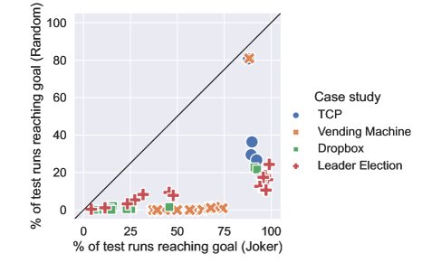
Figure 13: Joker-based versus randomized testing: percentage of tests reaching goal.

Figure 14 shows the experimental results for computation (2). To construct the graph, we computed for each goal, and separately for the sets of Joker test cases and random test cases, the average number of actions for reaching the goal. Hence, for each goal we obtain two average numbers: a number $r$ for the random test cases, and a number $j$ for the Joker test cases. For each goal, we then obtain the ratio $r/j$. If a test case did not reach a goal, the test case is not used to compute the average, so e.g. if $x$ out of the 10.000 test cases reached the goal, the average number of moves is computed from the number of moves of the $x$ test cases.

One bar in Figure 14 represents one case study, with all its goals. The black line depicts the variation between the ratios for the goals. Hence, we see that for all case studies but the Vending Machine, the ratios are close to each other. A possible reason for the high variation of ratios for the Vending Machine case study, is that we can see in Figure 13 that there are especially few random test cases that reach the goals of the Vending Machine case study, such that the average is computed over the number of moves of those few test cases. Moreover, we omitted results for 5 goal states of the Vending Machine case study, as these states were not reached in any of the 10.000 runs of random testing, while there were $>3500$ successful Joker runs for each of those goals. In general, for all the case studies, we see that the ratio is above 1, meaning that the Joker test cases use less moves than the random test cases.

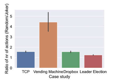
Figure 14: Ratio of average number of moves to the goals, where the average number of the random test cases is divided by the average number of the Joker test cases.

The overall conclusion from the graphs of Figure 13 and Figure 14 is that the Joker test cases clearly outperform the random test cases, both in reaching goal states, and the number of moves needed to reach a goal state. Our experimental results can be reproduced with the artefact [1].

9 Conclusions

We introduced the notion of Joker games, showed that its attractor-based Joker strategies use a minimum number of Jokers, and proved properties on determinacy, minimization of number of moves, randomization, and admissible strategies in the context of Joker games. In experiments we showed the effectiveness of Joker strategies when applied in model-based testing.

In future work, we would like to extend the experimental evaluation of Joker strategies on applications, and investigate more cost-minimal strategies. For example, we would like to also find the cost-minimal strategies that are currently not found via the Joker attractor construction. Furthermore, we are interested in other multi-objective strategies than our Joker distance strategies, i.e. strategies that are cost-minimal and also optimized for some other goal. Specifically, inspired by [14], we would like to investigate how to select and construct the Joker strategies that are the most robust against ‘bad’ opponent actions. Such ‘bad’ actions could e.g. move the game to a state where the game cannot be won anymore, or to a state from where many Jokers need to be spend to reach the goal.

Appendix

Appendix 0.A Proofs

*

Proof. First consider case $q\notin\textit{JAttr}({G},R)$. By Definition 11 we then have that $J\textit{Rank}(q)=\infty$. By Theorem 4 we have $q\notin{\textit{Reach}({G},R)}$. Hence $q$ cannot reach goal $R$ with any play. By Definition 8, we then have that any play has cost $\infty$, so any strategy has cost $\infty$, and then $\textit{Cost}(q)=\infty.$ Hence, $J\textit{Rank}(q)=\textit{Cost}(q)$.

Now consider $q\in\textit{JAttr}({G},R)$, so $q\in{\textit{Reach}({G},R)}$. By Definition 14 we then have a Joker attractor strategy. By Theorem 5, this strategy is cost-minimal. By Theorem 4 it uses $J\textit{Rank}(q)$ Jokers in any play, so its cost is $J\textit{Rank}(q)$. Since $\textit{Cost}(q)$ is defined as the cost of cost-minimal strategies (Definition 8), we have that $J\textit{Rank}(q)=\textit{Cost}(q)$.

*

Proof.

(1) We first prove lemma (W): $\sigma_{1}^{J}$ is a winning strategy in Joker game ${{G}^{\varspadesuit}}$. Let $q^{\prime}$ be a state in a play of $\textit{Outc}(\sigma_{1}^{J})$. Observe the following three cases:

• If $q^{\prime}\in\textit{Attr}({G},R)$, then $\sigma_{1}^{J}$ is a classical attractor strategy from $q$ that is winning [16], so reaches $R$, without using any Joker actions.

• If $q^{\prime}\in\textit{JAttr}^{k}({G},R)\setminus\textit{JAttr}_{\spadesuit}({G},R)$, $q^{\prime}$ is a non-Joker state of the $k$-th Joker attractor set, such that $\sigma_{1}^{J}$ is a classical attractor strategy from $q^{\prime}$ with goal $\textit{JAttr}^{k}_{\varspadesuit}({G},R)$. Hence, $\sigma_{1}^{J}$ will surely reach one of the Joker states $\textit{JAttr}^{k}_{\varspadesuit}({G},R)$, without using any Joker actions.

• If $q^{\prime}\in\textit{JAttr}_{\spadesuit}({G},R)$, then by the definition of a Joker attractor strategy (Definition 14), $\sigma_{1}^{J}$ uses a Joker action derived from the predecessor Pre, such that the Joker action causes the game to reach state $q^{\prime\prime}\in\textit{JAttr}^{k}({G},R)$ from $q^{\prime}\notin\textit{JAttr}^{k}({G},R)$. The use of $\textit{Pre}_{w}$ in the definition of a Joker attractor strategy (Definition 14) exactly corresponds with the use of Pre in the definition of the Joker attractor (Definition 11), so we have $J\textit{Rank}(q^{\prime\prime})+1=J\textit{Rank}(q^{\prime})$, and spend 1 Joker action making this move.

Consequently, $\sigma_{1}^{J}$ is a winning strategy, so (W) holds. Moreover, using 1 Joker action, reduces the rank of the next state by 1. Using the attractor in non-Joker states, costs no Joker actions. Since each of the $J\textit{Rank}(q)$ encountered Joker states we use 1 Joker action, we spend exactly $J\textit{Rank}(q)$ Joker actions in total.

2) By Theorem 5 we have that a Joker attractor strategy is cost-minimal, so any other cost-minimal strategy must have cost $J\textit{Rank}(q)$. That the cost can be less than $J\textit{Rank}(q)$ for some plays follows from Figure 4.

*

Proof.

To prove ${\textit{Reach}({G},R)}\subseteq\textit{WinReg}({{G}^{\varspadesuit}},R)$, we observe that a state $q^{\prime}\in R$ that can be reached from a state $q$ has a play $q_{0}\langle a_{0},x_{0}\rangle q_{1}\dots q_{n}$ with $q_{0}=q$ and $q_{n}=q^{\prime}$. This play allows constructing the winning strategy $\sigma\in\Sigma_{1}^{\varspadesuit}(q)$ in the Joker game, that only plays Joker actions to imitate the play: $\sigma(q_{0}\dots q_{k})=(a_{k},x_{k},q_{k+1})$ for all $0\leq k<n$ in ${{G}^{\varspadesuit}}$.

We conclude $\textit{WinReg}({{G}^{\varspadesuit}},R)\subseteq{\textit{Reach}({G},R)}$ from the three facts that (1) a state with a winning strategy in ${{G}^{\varspadesuit}}$ has a play reaching $R$, and (2) ${{G}^{\varspadesuit}}$ has the same states as ${G}$, and (3) playing a Joker action in ${{G}^{\varspadesuit}}$ corresponds to a regular move in ${G}$.

From lemma (W) from the proof of Theorem 4(1) we can derive that any state in $\textit{JAttr}({G},R)$ has a winning strategy in ${{G}^{\varspadesuit}}$, so $q\in\textit{WinReg}({{G}^{\varspadesuit}},R)$. Consequently we have: $\textit{JAttr}({G},R)\subseteq\textit{WinReg}({{G}^{\varspadesuit}},R)$.

Lastly, to prove that ${\textit{Reach}({G},R)}\subseteq\textit{JAttr}({G},R)$, we observe that $q\in(\textit{Pre})^{k}(\textit{JAttr}({G},R))\iff q\in\textit{JAttr}({G},R)$ for any $k\in\mathbb{N}$ by the definition of $\textit{JAttr}({G},R)$ (Definition 11). For any $q\in{\textit{Reach}({G},R)}$, we must have $q\in(\textit{Pre})^{k}(\textit{JAttr}({G},R))$ for some $k\in\mathbb{N}$, as $q$ can reach $R$ in a finite number of steps, because $Q$ is finite. Consequently, we have $q\in\textit{JAttr}({G},R)$ too.

From above $\subseteq$-relations the stated equalities follow trivially.

*

Proof.

(a) Let $q\in Q$ be a state and let $\sigma\in\Sigma_{1}(q)$ be a Joker attractor strategy according to Definition 14.

First suppose that $q\notin\textit{JAttr}({G},R)$. Then $q\notin{\textit{Reach}({G},R)}$ by Theorem 4, so $q$ has no winning play. Then any strategy – also $\sigma$ – has $\textit{Cost}(\sigma)=\infty$ by Definition 8. Consequently, $\sigma$ is cost-minimal.

Now suppose that $q\in\textit{JAttr}({G},R)$. We prove that $\sigma$ is cost-minimal by induction on $k=J\textit{Rank}(q)$.

If $k=0$, then $\sigma$ is a standard attractor strategy that does not spend any Joker actions, so $\textit{Cost}(\sigma)=0$. A Joker game has no actions with negative costs, so trivially, $\sigma$ is cost-minimal.

For $k>0$, we have the induction hypothesis that any Joker strategy $\sigma^{\prime}\in\Sigma_{1}(q^{\prime})$ with $J\textit{Rank}(q^{\prime})=m$ for $m<k$ is cost-minimal.

If $q\in\textit{JAttr}_{\spadesuit}({G},R)$, then $\sigma$ uses a Joker action $(a,x,q^{\prime\prime})$ with $(q,(a,x,q^{\prime\prime}))\in w\textit{JAttr}({G},R)$. By Definition 13 we have that $q^{\prime\prime}\in\textit{JAttr}^{m}({G},R)$ for $m<k$, so $\sigma$ is cost-minimal when starting in $q^{\prime\prime}$. By the Joker attractor construction we know that there is no possibility to reach $q^{\prime\prime}$ (or any other state in $\textit{JAttr}^{m}({G},R)$) from $q$ for sure (i.e. against any Player 2 and 3), because $q$ is not in the controllable predecessor of $\textit{JAttr}^{m}({G},R)$. So Player 2 or 3 can prevent Player 1 from winning if she uses no Joker action, which would yield a path, and corresponding strategy, with cost $\infty$ . Hence, using one Joker action is the minimum cost for reaching a state in $\textit{JAttr}^{m}({G},R)$. Consequently, $\sigma$ is cost-minimal in this case.

If $q\notin\textit{JAttr}_{\spadesuit}({G},R)$, then $\sigma$ is a standard attractor strategy attracting to a Joker state of $\textit{JAttr}^{k}({G},R)$. These standard attractor actions have cost 0. Upon reaching a Joker state, the same reasoning as above applies: we need to spend one Joker action. Hence, $\sigma$ is also cost-minimal in this case.

(b) See Figure 5.

*

Proof. This follows from Theorem 4:

• In any state $q\in\textit{JAttr}({G},R)$ we have a winning Player 1 strategy.

• From any $q\notin\textit{JAttr}({G},R)$, no state of $R$ can be reached, so Player 2 wins with any strategy.

*

Proof.
See Figure 6.

*

Proof.
(1) See Figure 8.

(2) Global cost-minimal strategies will, if possible, only use actions such that Player 2 and 3 cannot prevent Player 1 from winning, so we only need to consider states where Player 1 is not in full control: the Joker states. (If there are no Joker states, then any Joker-inspired cost-minimal strategy is winning.) We also note that Player 1 strategies that are not cost-minimal will not be able to do better, since at least the cost-minimal number of Joker states need to be passed by a play to a goal. From any Joker state $q$, the game continues to a state $q^{\prime}$, where either three of the following conditions hold:

1. $q^{\prime}\notin{\textit{Reach}({G},R)}$, i.e. Player 1 can never win the game any more.

2. $J\textit{Rank}(q)>J\textit{Rank}(q^{\prime})$, i.e. Player 1 got help from Player 2 and/or 3 to progress towards the goal.

3. $q^{\prime}\in\textit{JAttr}({G},R)$ and $J\textit{Rank}(q)<=J\textit{Rank}(q^{\prime})$, i.e. Player 1 is prevented to make progress.

Note that, for any Player 1 action, there is a Player 2 and a Player 3 action that forces the game to a state of type (1) or (3), because otherwise $q$ would not have been a Joker state. Joker-inspired global cost-minimal strategies will only propose Player 1 actions that also have a Player 2 and a Player 3 action such that the game moves to a state of type (2). Because the Player 2 and 3 strategies are positional, their choice for the type of the next state, is fixed, given a Player 1 action.

Hence, we draw the following conclusion (C): if two Player 1 strategies choose the same action, the next state of the game is the same. If two Player 1 strategies choose a different Player 1 action, then, depending on the game topology (i.e. the moves from state $q$), Player 2 and 3 either need to continue to the same type of state for any Player 1 action, or there are Player 2 and 3 strategies to make one Player 1 strategy continue to a type (2) state and the other to a (1) or (3) state, and vice versa (because $q$ is a Joker state, so Player 1 cannot force the game to a type (2) state for any enabled Player 1 action).

Consequently, we have a subset of Joker states $Q_{1}\subseteq\textit{JAttr}_{\spadesuit}({G},R)$, where Player 2 and 3 can force the game to a type (1) state, where Player 1 cannot win (i.e. cannot ever reach a goal state). Furthermore we have a subset of Joker states $Q_{3}\subseteq\textit{JAttr}_{\spadesuit}({G},R)$, where Player 2 and 3 can only force the game to a type (3) state, but, after a finite number of moves, Player 2 and 3 can force the game to visit a state from $Q_{1}$ for any Player 1 strategy that attempts to reach a goal state (i.e. our global cost-optimal strategies).

For the remaining set of Joker states $Q_{3}^{\prime}=\textit{JAttr}_{\spadesuit}({G},R)\setminus(Q_{1}\cup Q_{3})$, we show that Player 2 and 3 can force the game into a cycle, for any Player 1 strategy where Player 2 and 3 cannot force the game to a state of $Q_{1}\cup Q_{3}$. Concretely, in any state $q\in Q_{3}^{\prime}$, we have the following observation: Player 2 and 3 must be able to force the game to the same or another state $q^{\prime}\in Q_{3}^{\prime}$. Hence, we can think of this as a graph problem, where we have a finite set of nodes $Q_{3}^{\prime}$, and each node needs to have an outgoing directed edge to a node of $Q_{3}^{\prime}$. The analysis of this problem is as follows. When trying to add an edge $e$ for each node $n$, one by one, without making a cycle, one has to connect the edge from $n$ to a node that does not have and outgoing edge yet, because otherwise we create a cycle via $e$. Because the set $Q_{3}^{\prime}$ is finite, the last added edge needs to go to a node that already has an outgoing edge. Consequently this creates a cycle anyway. Hence, also in Joker states $Q_{3}^{\prime}$ Player 2 and 3 have a strategy such that Player 1 does not ever reach a goal state, as the game is kept in a cycle forever.

Consequently, from any Joker state, Player 2 and 3 have a strategy against any Player 1 strategy, such that a goal state is never reached. Also, Player 2 and 3 have a strategy that allows any global cost-minimal Player 1 strategy to reach a goal state. Because the Player 2 and 3 strategies need to be positional, such a pair fixes the choice of Player 2 action and next state, for a given Player 1 action and current state. Hence, only global cost-minimal Player 1 strategies that choose different actions in Joker states, or steer the game to different Joker states via non-Joker states, may have different winning sets of Player 2 and 3 strategies.

This leads to the generalized conclusion C: two global cost-minimal Player 1 strategies either have the same pairs of winning Player 2 and 3 strategies, or for each of the two Player 1 strategies there is a pair of winning Player 2 and 3 strategies the other strategy cannot win from. Hence, each of the two global cost-minimal Player 1 strategies does not dominate the other strategy. Strategies that are not global cost-minimal will not be able to dominate either, as they also will have to pass a Joker state towards a goal state. Consequently, global cost-optimal strategies are admissible.

*

Proof.
(a)

The following observation provides the foundation for below proof: When a Joker state $q$ is added to a set $\textit{dJAttr}^{k}({G},R)$ of the Joker distance attractor (Definition 20) by the distance predecessor dPre (Definition 19), the definition of dPre requires the following when adding a state $q$:

• When $J\textit{Rank}(q)=J\textit{Rank}(q^{\prime})+1$, $q$ must have been added for some Joker move from $q$ to $q^{\prime}$, since this part of the definition (i.e. $\exists a\in\Gamma_{1}(q),\exists x\in\Gamma_{2}(q),\exists q^{\prime}\in\textit{Moves}(q,a,x):q^{\prime}\in Q^{\prime}$) is exactly the predecessor Pre operation of Definition 9.

• When $J\textit{Rank}(q)=J\textit{Rank}(q^{\prime})$, $q$ is added for some controlled move from $q$ to $q^{\prime}$, since this part of the definition (i.e. $\exists a\in\Gamma_{1}(q),\forall x\in\Gamma_{2}(q):\textit{Moves}(q,a,x)\subseteq Q^{\prime}$) is exactly the controlled predecessor of Definition 9. So , the rank of the states via the controlled predecessor remain the same, and no Joker action is used.

Now we do a proof by induction to show that Joker distance strategies are cost-minimal. Let $\sigma\in\Sigma(q^{0})$ be a Joker distance strategy for Joker game ${{G}^{\varspadesuit}}$ with initial state $q^{0}\in\textit{JAttr}({G},R)$. Let $J\textit{Rank}(q^{0})=n$ for some $n\in\mathbb{N}$.

• First suppose $n=0$. Because the Joker attractor added $q^{0}$ via controlled predecessor operations only, this must be the case for the Joker distance predecessor too. Hence, the resulting strategy will enforce a play with states $q^{0},q^{\prime},...,r$, where $r\in R$, all states have rank 0, and 0 Joker actions are used. Then trivially $\sigma$ is cost-minimal.

• Now suppose that $n>0$. From the induction hypothesis we obtain that for any state $q^{\prime}$ with $J\textit{Rank}(q^{\prime})=n-1$, the Joker distance strategy $\sigma$ will use $J\textit{Rank}(q^{\prime})$ Jokers for any play starting from $q^{\prime}$, i.e., against any opponent. There must be a state $q^{\prime}$ with $J\textit{Rank}(q^{\prime})=n-1$ such that there is a play from $q$ to $q^{\prime}$, because $q\in\textit{JAttr}^{n}({G},R)$ and $q^{\prime}\in\textit{JAttr}^{n-1}({G},R)$. In particular, we know from the Joker attractor construction that we have a finite play $\pi$ from $q$ to $q^{\prime}$ with states $q,...,q^{\prime\prime},q_{j},q^{\prime\prime\prime},...,q^{\prime\prime\prime\prime},q^{\prime}$, such that $q^{\prime\prime\prime},...,q^{\prime\prime\prime\prime}$ are obtained via the controlled predecessor, then state $q_{j}$ via the predecessor, i.e. via a Joker move, and states $q,..q.,q^{\prime\prime}$ via the controlled predecessor again. Because the Joker distance predecessor adds states also via the predecessor or controlled predecessor, while ensuring a rank increase of 1 only occurs when applying the predecessor, and otherwise remains equal, $q$ must also have be added to the Joker distance attractor at some iteration, though the intermediate states added can be different than those in $\pi$ (and hence the corresponding strategy differs). The consequence is that the Joker distance attractor will have witnesses for moves from $q$ to $q^{\prime}$ such that only one Joker action is used. By the induction hypothesis we then obtain that the Joker distance strategy uses $n$ Jokers from $q^{0}$.

Since Joker strategies are cost-minimal (Theorem 5), and since have proven that Joker distance strategies use the same number of Joker actions, we obtain that Joker distance strategies are cost-minimal.

(b) We observe that the Joker distance predecessor selects all states that can be added via both the predecessor and the controlled predecessor. The Joker attractor either uses the controlled predecessor or the predecessor to add states. Consequently, the witnessed Joker distance attractor considers all and more winning plays in the Joker game than the witnessed Joker attractor. Moreover, the Joker distance attractor minimizes the distance of the selected moves because of its attractor structure, where its rank is the distance. Therefore a Joker distance strategy uses the same or less moves than a Joker strategy for any play.

*

Proof.

This follows from a result of [7]. They define a set of states $Sure(R)$ that have a sure winning strategy (win against any opponent), i.e. this corresponds to $\textit{Attr}({G},R)$ in our notation. They furthermore define a set of states $Almost(R)$ that have an almost sure winning strategy (win against any opponent with probability 1), i.e. this corresponds to $\textit{pAttr}_{1}({G},R)$ in our notation. The result of [7] is then that $Sure(R)\subseteq Almost(R)$. Hence, the probabilistic attractor consists of the same or more states than the standard attractor. The result is that states that are Joker states according to the Joker attractor may be included in the probabilistic attractor. The probabilistic Joker attractor then finds that the initial state has a lower Joker rank, than with the Joker attractor, such that the randomized winning strategies $\sigma$ in the Joker game use less Jokers than Joker attractor strategies $\sigma^{\prime}$. Figure 12 shows that games exist for which this occurs. In the other cases (since $Sure(R)\subseteq Almost(R)$), the probabilistic attractor and standard attractor yield the same set of states. Hence, we have for randomized Joker strategies $\sigma$ and Joker attractor strategies $\sigma^{\prime}$ that $\textit{Cost}(\sigma)\leq\textit{Cost}(\sigma^{\prime})$.

*

Proof.

(1) We can follow the original proof of Theorem 4(1), and only make the following two changes to use it in the setting of randomized strategies:

• In case $q^{\prime}\in\textit{Attr}({G},R)$, we have that $\sigma_{1}^{J}$ is a probablistic attractor strategy from $q$ that is almost sure winning, i.e. reach R with probability 1, without using any Joker actions.

• In case $q^{\prime}\in\textit{JAttr}^{k}({G},R)\setminus\textit{JAttr}_{\spadesuit}({G},R)$, we similarly have a probablistic attractor strategy now, that almost surely reaches one of the Joker states without using any Joker actions.

(2) follows from Theorem 7.3 as in the original proof of Theorem 4(2).

*

Proof. We follow the proof of Theorem 4 with the following changes:

• In the proof of case ${\textit{Reach}({G},R)}\subseteq\textit{WinReg}({{G}^{\varspadesuit}},R)$ we adapt the strategy $\sigma$ to play the proposed Joker actions with probability 1.

• In the proof of case $\textit{WinReg}({{G}^{\varspadesuit}},R)\subseteq{\textit{Reach}({G},R)}$, we use for fact (1) that there is an almost sure winning strategy, and in fact (3) we use a Joker action that is played with probability 1 .

• The proof of case $p\textit{JAttr}({G},R)\subseteq\textit{WinReg}({{G}^{\varspadesuit}},R)$ uses lemma (W) of Theorem 4(1) as described for this case in Theorem 4. But in lemma (W) we substitute Attr by pAttr, $\textit{JAttr}({G},R)$ by $p\textit{JAttr}({G},R)$, and $J\textit{Rank}$ by $pJ\textit{Rank}$.

• In the proof of case ${\textit{Reach}({G},R)}\subseteq p\textit{JAttr}({G},R)$, we need no changes, as the definition of $p\textit{JAttr}({G},R)$ uses Pre also when $\textit{pAttr}_{1}({G},R)$ is used instead of $\textit{Attr}({G},R)$.

*

Proof. We follow the proof of Theorem 5, but use the probabilistic definitions at all places in this proof. Hence we adapt the proof as follows:

• We define $\sigma\in\Sigma_{1}^{r}(q)$ as a randomized Joker strategy.

• In the first case we suppose that $q\notin p\textit{JAttr}({G},R)$, and use Theorem 7.3 instead of Theorem 4.

• In the second case we take $q\in p\textit{JAttr}({G},R)$ and prove that $\sigma$ is cost-minimal by induction on $k=pJ\textit{Rank}(q)$.

  • In case $k=0$ we use a randomized Joker strategy (Definition 28) instead of a standard attractor strategy, and similarly use no Joker actions, so $\sigma$ is cost-minimal.

  • In case $k>0$ we have the induction hypothesis that any $\sigma^{\prime}\in\Sigma_{1}^{r}(q^{\prime})$ with $pJ\textit{Rank}(q^{\prime})=m$ for $m<k$ is cost-minimal.

    • If $q\in p\textit{JAttr}_{\spadesuit}({G},R)$, then $\sigma$ uses a Joker action $(a,x,q^{\prime\prime})$ with $(q,(a,x,q^{\prime\prime}))\in wp\textit{JAttr}({G},R)$. By Definition 30 we have that $q^{\prime\prime}\in p\textit{JAttr}^{m}({G},R)$, so $\sigma$ is cost-minimal when starting in $q^{\prime\prime}$. By the probabilistic Joker attractor construction we know that there is no possibility to reach $q^{\prime\prime}$ from $q$ with probability 1, because $q$ has been excluded by $\mathit{Safe}_{1}$ at some point. For same reasons as in the proof of Theorem 5 it is minimum cost to spend 1 Joker action, so $\sigma$ is cost-minimal in this case.

    • If $q\notin p\textit{JAttr}_{\spadesuit}({G},R)$ then $\sigma$ is a randomized Joker strategy to a Joker state of $p\textit{JAttr}^{k}({G},R)$, using 0 cost actions only. Upon reaching a Joker state we follow the above reasoning. Hence $\sigma$ is also cost-minimal in this case.

*

Proof. Similar to the proof of Theorem 5 this follows from Theorem 7.3.

*

Proof. Let $\sigma_{1}\in\Sigma_{1}^{r}(q^{0})$ be an almost sure winning randomized strategy.
1) Then there is a winning play in $\textit{Outc}(\sigma_{1})$. As in the proof of Theorem 4, we can use this play for constructing a strategy that plays the Joker actions matching the play.
2) Because we use the probabilistic Joker attractor (Definition 28), in each probabilistic Joker attractor set, we can attract with probability 1 to a Joker state [7]. In a Joker state $q$ we choose Joker action $(a,x,q^{\prime})$ such that $pJ\textit{Rank}(q)>pJ\textit{Rank}(q^{\prime})$ with probability 1. By choosing such a move in a Joker state, the game moves to a state with a smaller Joker rank with probability 1. Decreasing the Joker rank in each Joker state leads to reaching a goal state. Because a next Joker state is reached with probability 1 each time, the overall probability of the resulting strategy is 1 too, so it is almost sure winning.
3) See the proof of 2).

*

Proof. This is exactly what we use in the proof of Theorem 7.4(2).

References

- [1] The artefact of this paper for reproducing the experimental results of Section 8. https://doi.org/10.5281/zenodo.7712109.
- [2] Ezio Bartocci, Roderick Bloem, Benedikt Maderbacher, Niveditha Manjunath, and Dejan Ničković. Adaptive testing for specification coverage in CPS models. IFAC-PapersOnLine, 54(5):229–234, 2021. 7th IFAC Conference on Analysis and Design of Hybrid Systems ADHS 2021.
- [3] Catriel Beeri. On the membership problem for functional and multivalued dependencies in relational databases. ACM Trans. Database Syst., 5(3):241–259, 1980. doi:10.1145/320613.320614.
- [4] D.P. Bertsekas. Dynamic Programming and Optimal Control. Athena Scientific, 1998.
- [5] Dietmar Berwanger. Admissibility in infinite games. In STACS 2007 – Symposium on Theoretical Aspects of Computer Science, Proceedings, LNCS. Springer, 2007.
- [6] Roderick Bloem, Rüdiger Ehlers, and Robert Könighofer. Cooperative reactive synthesis. In Automated Technology for Verification and Analysis - 13th International Symposium, ATVA 2015, Shanghai, China, October 12-15, 2015, Proceedings, volume 9364 of Lecture Notes in Computer Science, pages 394–410. Springer, 2015.
- [7] Benjamin Bordais, Patricia Bouyer, and Stéphane Le Roux. Optimal Strategies in Concurrent Reachability Games. In 30th EACSL Annual Conference on Computer Science Logic (CSL 2022), volume 216 of Leibniz International Proceedings in Informatics (LIPIcs), pages 7:1–7:17, 2022.
- [8] Petra van den Bos and Marielle Stoelinga. Tester versus bug: A generic framework for model-based testing via games. 277:118–132, 2018. URL: https://doi.org/10.48550/arXiv.1809.03098.
- [9] Petra van den Bos and Frits Vaandrager. State identification for labeled transition systems with inputs and outputs. Science of Computer Programming, 209:102678, 2021.
- [10] Romain Brenguier, Lorenzo Clemente, Paul Hunter, Guillermo A. Pérez, Mickael Randour, Jean-François Raskin, Ocan Sankur, and Mathieu Sassolas. Non-zero sum games for reactive synthesis. In Adrian-Horia Dediu, Jan Janoušek, Carlos Martín-Vide, and Bianca Truthe, editors, Language and Automata Theory and Applications, pages 3–23, Cham, 2016. Springer.
- [11] Romain Brenguier, Guillermo A. Pérez, Jean-François Raskin, and Ocan Sankur. Admissibility in quantitative graph games. CoRR, abs/1611.08677, 2016.
- [12] Krishnendu Chatterjee and Thomas A. Henzinger. Assume-guarantee synthesis. In Proceedings of the 13th International Conference on Tools and Algorithms for the Construction and Analysis of Systems, volume 4424 of Lecture Notes in Computer Science, pages 261–275. Springer, 2007.
- [13] ComMA: Introductory ComMA tutorial. https://www.eclipse.org/comma/tutorial/intro.html.
- [14] Eric Dallal, Daniel Neider, and Paulo Tabuada. Synthesis of safety controllers robust to unmodeled intermittent disturbances. In Decision and Control (CDC), 2016 IEEE 55th Conference on, pages 7425–7430. IEEE, 2016.
- [15] Alexandre David, Kim G Larsen, Shuhao Li, and Brian Nielsen. A game-theoretic approach to real-time system testing. In Design, Automation and Test in Europe, 2008. DATE’08, pages 486–491. IEEE, 2008.
- [16] Luca de Alfaro, Thomas A. Henzinger, and Orna Kupferman. Concurrent reachability games. In FOCS ’98: Proceedings of the 39th Annual Symposium on Foundations of Computer Science, page 564. IEEE Computer Society, 1998.
- [17] Luca de Alfaro and Mariëlle Stoelinga. Interfaces: A game-theoretic framework for reasoning about component-based systems. Electron. Notes Theor. Comput. Sci., 97:3–23, 2004.
- [18] Marco Faella. Admissible strategies in infinite games over graphs. In Rastislav Královič and Damian Niwiński, editors, Mathematical Foundations of Computer Science, pages 307–318. Springer, 2009.
- [19] Paul Fiterău-Broştean, Ramon Janssen, and Frits Vaandrager. Combining model learning and model checking to analyze TCP implementations. In S. Chaudhuri and A. Farzan, editors, Computer Aided Verification, pages 454–471, Cham, 2016. Springer.
- [20] Wan Fokkink. Distributed algorithms - an intuitive approach, second edition, 2018.
- [21] Anders Hessel, Kim Guldstrand Larsen, Marius Mikucionis, Brian Nielsen, Paul Pettersson, and Arne Skou. Testing real-time systems using UPPAAL. In Formal Methods and Testing, An Outcome of the FORTEST Network, Revised Selected Papers, pages 77–117, 2008.
- [22] John Hughes, Benjamin Pierce, Thomas Arts, and Ulf Norell. Mysteries of Dropbox: Property-based testing of a distributed synchronization service. In 2016 IEEE International Conference on Software Testing, Verification and Validation (ICST), pages 135–145. IEEE, 2016.
- [23] Ivan Kurtev., Mathijs Schuts., Jozef Hooman., and Dirk-Jan Swagerman. Integrating interface modeling and analysis in an industrial setting. In Proceedings of the 5th International Conference on Model-Driven Engineering and Software Development - MODELSWARD,, pages 345–352. INSTICC, SciTePress, 2017.
- [24] Daniel Neider, Alexander Weinert, and Martin Zimmermann. Synthesizing optimally resilient controllers. Acta Informatica, 57(1-2):195–221, 2020.
- [25] Jan Tretmans and Michel van de Laar. Model-based testing with TorXakis: The mysteries of Dropbox revisited. In V. Strahonja, editor, CECIIS : 30th Central European Conference on Information and Intelligent Systems, October 2-4, 2019, Varazdin, Croatia. Proceedings, pages 247–258. Zagreb: Faculty of Organization and Informatics, University of Zagreb, 2019.
- [26] Petra van den Bos and Mariëlle Stoelinga. With a little help from your friends: Semi-cooperative games via joker moves. In Marieke Huisman and António Ravara, editors, Formal Techniques for Distributed Objects, Components, and Systems - 43rd IFIP WG 6.1 International Conference, FORTE 2023, Held as Part of the 18th International Federated Conference on Distributed Computing Techniques, DisCoTec 2023, Lisbon, Portugal, June 19-23, 2023, Proceedings, volume 13910 of Lecture Notes in Computer Science, pages 155–172. Springer, 2023. doi:10.1007/978-3-031-35355-0\_10.
- [27] Quanyan Zhu, Tansu Alpcan, Emmanouil A. Panaousis, Milind Tambe, and William Casey, editors. Proceedings of the 7th International Conference, Decision and Game Theory for Security, volume 9996 of LNCS. Springer, 2016.
- [28] Wieslaw Zielonka. Infinite games on finitely coloured graphs with applications to automata on infinite trees. Theoretical Computer Science, 200(1):135 – 183, 1998.