Quantum-circuit algorithms for many-body topological invariant
and Majorana zero mode

Abstract

The topological state of matter is a potential resource to realize long-term fault-tolerant quantum computers beyond the near-term noisy intermediate-scale quantum devices. To achieve the realization, we need a deep understanding of topological behaviors in real quantum computers. However, quantum-circuit algorithms to analyze topological properties have still been insufficient. Here we propose three quantum-circuit algorithms, (i) to find the ground state in the selected parity subspace, (ii) to determine the many-body topological invariant, and (iii) to visualize the zero-energy edge mode. To demonstrate these algorithms, we adopt the interacting Kitaev chain as a typical model of many-body topological superconductors in one dimension. The algorithms are applicable to not only one-dimensional topological superconductors but other topological states including higher-dimensional systems.

I Introduction

The recent development of quantum computers makes us expect quantum supremacy or at least quantum advantage in the near future [1, 2, 3, 4]. Particularly, noisy intermediate-scale quantum (NISQ) devices based on the gate-type unitary operations are on the point of entering an unexplored region beyond the limit of numerical calculation that classical computers can approach in a feasible amount of time [3, 5, 6, 7]. In parallel, various quantum-circuit (QC) algorithms consisting of the quantum gates and supported by auxiliary calculations on classical computers have rapidly appeared for general use, e.g., quantum approximate optimization algorithm [8, 9, 10, 11, 12, 13, 14, 15], quantum Fourier transformation [16], quantum singular-value decomposition [17, 18, 19], and quantum machine learning [20, 21, 22, 23, 24, 25, 26, 27, 28, 29].

On the other hand, QC algorithms for condensed-matter research are not sufficient except for recently-proposed essential algorithms for the eigensystem of the model Hamiltonian, called the variational quantum eigensolver (VQE) [30, 31, 32, 33, 34, 35, 36, 37, 38, 39, 40, 41], and for the dynamics (temperature-dependence) using the real (imaginary) time evolution [42, 43, 44, 45, 46, 47, 48]. In fact, for analyzing topological properties, only a few algorithms have been proposed so far [26, 49, 50, 51]. To overcome the limitation of coherence time and to realize a fault-tolerant quantum computer (FTQC), a deep understanding of the topological state of matter in real quantum computers is crucial. Therefore, in this paper, we propose QC algorithms composed of three steps, (i) to find the ground state in selected parity subspace, (ii) to determine the many-body topological invariant, and (iii) to visualize the zero-energy edge mode.

For the demonstration of the algorithms, we adopt the interacting Kitaev chain as a one-dimensional topological superconductor with many-body interaction [52, 53, 54, 55, 56, 57, 58]. The Kitaev chain is a typical model of topological state belonging to the BDI class, i.e., conserving time-reversal, particle-hole, and chiral (sublattice) symmetries [59, 60]. In addition, introducing the many-body interaction induces the topological transition from non-trivial to trivial phases in terms of topological invariant. Besides, the topological superconducting state has a zero-energy edge mode composed of Majorana fermions (MF), called the Majorana zero mode (MZM). Since the MZM is a potential resource of the braiding type of topological quantum computing for the long-term FTQC [61, 62, 3], visualization of its behavior is also important from both fundamental and engineering points of view.

The rest of this paper consists of the following contents. In Sec. II, we define the model Hamiltonian of the interacting Kitaev chain as spinless-fermion representation, and present the Majorana and spin counterparts of it. As the first step of the QC algorithms, we adapt the VQE technique to find the ground state in the selected parity subspace in Sec. III, and show the numerical results of the algorithm. In Sec. IV, we briefly explain the topological invariant in the tight-binding (TB) and many-body (MB) model, i.e., without and with the interaction term, respectively. After the explanation, a QC algorithm to determine the MB topological invariant is proposed with the numerical results of it for various points in the model-parameter space, including topologically trivial and non-trivial states. Additionally, the MZM is numerically visualized by using the ground states in two different parity subspaces in several model-parameter points located in the topological phases. The numerical calculations in this paper have been done on the QC simulator, qulacs [63], in the classical computer. Finally, we summarize the present study and give a discussion about the advantages and disadvantages of our algorithms, with some caveats when we execute the algorithms in real NISQ devices.

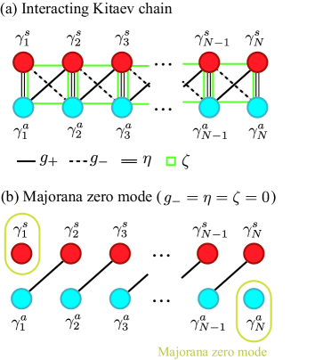
Figure 1: (a) Schematic of the interacting Kitaev chain. Four coupling terms, $g_{+}$, $g_{-}$, $\eta$, and $\zeta$ are denoted by solid lines, dashed lines, and double solid lines, and green squares, respectively. (b) Majorana zero mode (MZM) for $g_{-}=\eta=\zeta=0$. Two MFs $\gamma_{1}^{s}$ and $\gamma_{N}^{a}$ at the edges are decoupled from the system, corresponding to the MZM.

II Model

In this section, we introduce the model Hamiltonian of one-dimensional topological superconductor, the so-called Kitaev chain with the attractive interaction on neighboring bonds [52, 55, 56, 57, 58]. The model Hamiltonian with the open boundary condition (OBC) for the $N$-site system is defined by,

$$\mathcal{H}_{\mathrm{K}}= -t\sum_{j=1}^{N-1}\left(c^{\dagger}_{j}c_{j+1}+\mathrm{H.c.}\right)-\Delta\sum_{j=1}^{N-1}\left(c^{\dagger}_{j}c_{j+1}^{\dagger}+\mathrm{H.c.}\right)$$

$$-V\sum_{j=1}^{N-1}\left(n_{j}-\frac{1}{2}\right)\left(n_{j+1}-\frac{1}{2}\right)-\mu\sum_{j=1}^{N}\left(n_{j}-\frac{1}{2}\right),$$ (1)

where $c_{j}$, $c_{j}^{\dagger}$, and $n_{j}$ denote annihilation, creation, and number operators of spinless fermion at $j$th site, respectively. In addition, the hopping integral, the superconducting pairing potential, and the Coulomb potential between neighboring sites are given by $t$, $\Delta$, and $V$, respectively, with the chemical potential $\mu$. In this paper, we focus on the attractive region for the Coulomb potential $V>0$, to avoid the trivial phase of the repulsive region, where the translational symmetry is spontaneously broken [56, 57, 58]. Without the interaction, we can easily understand the topological invariant and the MZM, based on the one-particle picture (see Section IV for the topological invariant and Section V for the MZM).

The Kitaev chain mathematically corresponds to the $S=1/2$ XYZ spin chain,

$$\mathcal{H}_{\mathrm{S}}=-\sum_{\alpha=x,y,z}J_{\alpha}\sum_{j=1}^{N-1}S_{j}^{\alpha}S_{j+1}^{\alpha}-h_{z}\sum_{j=1}^{N}S_{j}^{z},$$ (2)

via the Jordan–Wigner (JW) transformation,

$$c_{j}=S_{j}^{-}e^{\imath\varphi_{j}},\ c_{j}^{\dagger}=S_{j}^{+}e^{\imath\varphi_{j}},\ n_{j}=S_{j}^{z}+\frac{1}{2}.$$ (3)

The JW phase is defined by $\varphi_{j}=\pi\sum_{i=1}^{j-1}(S_{i}^{z}+\frac{1}{2})$ with the imaginary unit $\imath=\sqrt{-1}$, and $S_{j}^{\alpha}$ ($S_{j}^{\pm}$) represents the $\alpha=x,y,z$ component of $S=1/2$ spin operator (the ladder operator of spin) at $j$th site with the natural unit $\hbar=1$. The anisotropic exchange interaction is denoted by $J_{\alpha}$, and $h_{z}$ represents the magnetic field along $z$ axis. The coupling terms in the Kitaev chain and the XYZ spin chain have the following relations:

$$t=\frac{J_{x}+J_{y}}{4},\ \Delta=\frac{J_{x}-J_{y}}{4},\ V=J_{z},\ \mu=h_{z}.$$ (4)

Since the QC is compatible to the spin representation, we mainly use the spin representation of the Hamiltonian in this paper.

To understand topological properties in the Kitaev chain, the MF representation is important. The MF representation of the Kitaev chain (II) is given by,

$$\mathcal{H}_{\mathrm{M}}=\, -\imath g_{-}\sum_{j=1}^{N-1}\gamma_{j}^{s}\gamma_{j+1}^{a}+\imath g_{+}\sum_{j=1}^{N-1}\gamma_{j}^{a}\gamma_{j+1}^{s}$$

$$+\zeta\sum_{j=1}^{N-1}\gamma_{j}^{s}\gamma_{j}^{a}\gamma_{j+1}^{s}\gamma_{j+1}^{a}-\imath\eta\sum_{j=1}^{N}\gamma_{j}^{s}\gamma_{j}^{a},$$ (5)

with the coupling constants $g_{\pm}=(t\pm\Delta)/2$, $\zeta=V/4$, and $\eta=\mu/2$. The symmetric ($\gamma_{j}^{s}$) and antisymmetric ($\gamma_{j}^{a}$) modes of MF at $j$th site are defined by,

$$\gamma_{j}^{s}=c_{j}^{\dagger}+c_{j},\quad\gamma_{j}^{a}=\imath\left(c_{j}^{\dagger}-c_{j}\right).$$ (6)

Note that the MF operators obey the fermionic anti-commutation relation $\{\gamma_{j}^{\tau},\gamma_{j^{\prime}}^{\tau^{\prime}}\}=2\delta_{j,j^{\prime}}\delta_{\tau,\tau^{\prime}}$ with the Hermiticy $(\gamma_{j}^{\tau})^{\dagger}=\gamma_{j}^{\tau}$ for $\tau(\tau^{\prime})=s,a$.

Figure 1(a) shows the schematic of the MF Hamiltonian (II). A pair of symmetric (red ball) and antisymmetric (blue ball) MFs corresponds to a spinless fermion. When $g_{-}=\eta=\zeta=0$, the $g_{+}$ diagonal coupling only remains, so that two MFs $\gamma_{1}^{s}$ and $\gamma_{N}^{a}$ at the edges are decoupled from the system. The pair of MFs, are regarded as a spinless fermion with zero energy, i.e., the MZM, causing two-fold degeneracy at every energy level. The existence of MZM is also an evidence of topological superconductor.

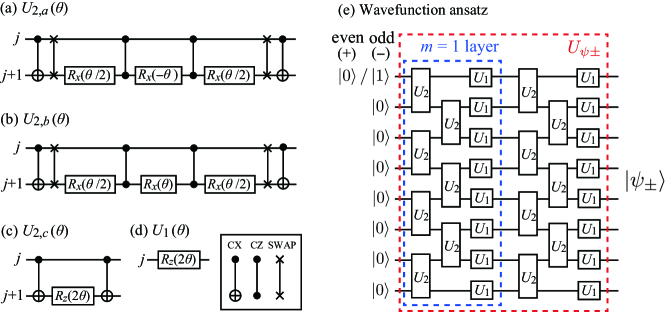
Figure 2: (a-d) QC representation of three unitary operators $U_{2,p}(\theta)$ for $p=a,b,c$ and $U_{1}(\theta)$, where one-qubit rotation around $\alpha=x,y,z$ axis is denoted by $R_{\alpha}(\theta)=\exp[\imath(\theta/2)\sigma^{\alpha}]$ with the Pauli matrix $\sigma^{\alpha}$. (e) Wavefunction ansatz for the parity-conserved VQE method ($N=8$, $M=2$). We adopt a Trotter-like QC constructed by the $U_{2}(\bm{\theta})=U_{2,a}(\theta_{a})U_{2,b}(\theta_{b})U_{2,c}(\theta_{c})$ and $U_{1}(\vartheta)$ gates with $\bm{\theta}=(\theta_{a},\theta_{b},\theta_{c})$. The angles $\bm{\theta}$ and $\vartheta$ are assigned to variational parameters for the VQE optimization. Thus, the total number of variational parameters is $N_{\theta}=(4N-3)M$ with the OBC.

III Ground state

Next, we explain how to obtain the ground states in the QC with conserving the fermion parity. Since the Kitaev chain has pair creation and annihilation terms [the second term in (II)], the total number of fermions $N=\sum_{j}n_{j}$ is not conserved. Instead, the fermion parity $\mathcal{F}=\exp[\imath\pi\sum_{j}n_{j}]=\pm 1$, i.e., whether the number of fermions is even or odd, is a good quantum number. The fermion parity corresponds to the magnetization parity $\mathcal{M}_{z}$ in the XYZ spin chain,

$$\mathcal{F}=\mathcal{M}_{z}=\imath^{N}\exp\left[\imath\pi\sum_{j}S_{j}^{z}\right]=(-\imath)^{N}\prod_{j}(2S_{j}^{z}).$$ (7)

It is worth noting that since the $\alpha=x,y,z$ components of spin operator $S_{j}^{\alpha}$ are introduced in the XYZ spin chain as the same form, there are other conversed quantities $\mathcal{M}_{\alpha}=\imath^{N}\exp[\imath\pi\sum_{j}S_{j}^{\alpha}]$ for $\alpha=x,y$, while the three parities are not independent due to the relation $\mathcal{M}_{x}\mathcal{M}_{y}\mathcal{M}_{z}=(-\imath)^{3N}\prod_{j}(8S_{j}^{x}S_{j}^{y}S_{j}^{z})=(-1)^{N}$ [64]. In this paper, to avoid misunderstanding due to the system-size dependence of the fermion parity, we consider only the system sizes satisfying $N=0$ (mod. $4$).

To implement the ground state into the QC, we use the parity-conserved 2-site unitary operator on $j$th bond defined by

$$U_{2}(\bm{\theta})=U_{2,a}(\theta_{a})U_{2,b}(\theta_{b})U_{2,c}(\theta_{c})$$ (8)

with

$$U_{2,a}(\theta) =\exp\left[2\imath\theta\left(S_{j}^{x}S_{j+1}^{x}+S_{j}^{y}S_{j+1}^{y}\right)\right]$$

$$=\exp\left[\imath\theta\left(S_{j}^{+}S_{j+1}^{-}+\mathrm{H.c.}\right)\right],$$ (9)

$$U_{2,b}(\theta) =\exp\left[2\imath\theta\left(S_{j}^{x}S_{j+1}^{x}-S_{j}^{y}S_{j+1}^{y}\right)\right]$$

$$=\exp\left[\imath\theta\left(S_{j}^{+}S_{j+1}^{+}+\mathrm{H.c.}\right)\right],$$ (10)

$$U_{2,c}(\theta) =\exp\left[4\imath\theta S_{j}^{z}S_{j+1}^{z}\right],$$ (11)

where the vector of angles includes three angles, $\bm{\theta}=(\theta_{a},\theta_{b},\theta_{c})$. Although the unitary operators $U_{2}$ and $U_{1}$ have the site dependence, we omit the site index $j$ in the notation of unitary operators (8) and (12) for simplicity. Note that these operators $U_{2,p}(\theta)$ ($p=a,b,c$) on the $j$th bond, commute with each other, $[U_{2,p}(\theta),U_{2,p^{\prime}}(\theta^{\prime})]=0$, while the unitary operators do not always commute between the neighboring bonds. In addition, to take into account the effect of magnetic field, we introduce the 1-site unitary operator at $j$th site given by

$$U_{1}(\theta)=R_{z}(2\theta)=\exp\left[2\imath\theta S_{j}^{z}\right].$$ (12)

Figure 2 shows the QC representation of these unitary operators. Since these operators preserve the fermion parity $[U_{2,p}(\theta),\mathcal{F}]=[U_{1}(\vartheta),\mathcal{F}]=0$, the fermion parity after the unitary operations equals the parity of the initial state.

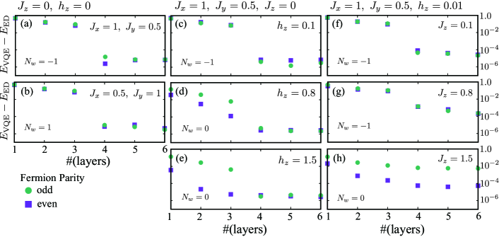
Figure 3: Energy differences between the VQE and the ED method in the 12-site XYZ spin chain. (a,b) Left panels show the XY anisotropy dependence without the magnetic field and the Ising term, $h_{z}=J_{z}=0$. (c-e) The field dependence with fixed $J_{y}/J_{x}=0.5$ and $J_{z}=0$ is shown in center panels. (f-h) Right panels show the Ising term (i.e., the Coulomb interaction in the Kitaev chain) dependence with fixed $J_{y}/J_{x}=0.5$ and $h_{z}=0.01$. To avoid degeneracy with large $J_{z}$ in topologically-trivial state, we add a small magnetic field $h_{z}=0.01$. $N_{w}$ represents the winding number explained in Sec. IV. The VQE energy is obtained as the minimal energy in 10-times VQE optimization trials from random initial angles.

By using the parity-conserved 2-site and 1-site unitary operators, we adopt the following wavefunction ansatz for the VQE method:

$$\ket{\psi_{\pm}(\{\bm{\theta}_{j,m},\vartheta_{j,m}\})}=U_{\psi\pm}\ket{\mathrm{i}_{\pm}},$$ (13)

with

$$U_{\psi\pm}=\prod_{m=1}^{M}\left[\prod_{j}U_{1}(\vartheta_{j,m})\prod_{\mathrm{even}\,j}U_{2}(\bm{\theta}_{j,m})\prod_{\mathrm{odd}\,j}U_{2}(\bm{\theta}_{j,m})\right]$$ (14)

and the initial state for even parity $\ket{\mathrm{i}_{+}}=\ket{0}^{\otimes N}$ or odd parity $\ket{\mathrm{i}_{-}}=\sigma_{1}^{x}\ket{\mathrm{i}_{+}}=\ket{1}\otimes\ket{0}^{\otimes N-1}$. $M$ is the number of layers (see the QC representation shown in Fig. 2), so that the total number of variational parameters (namely, the number of angles in unitary operators $\{\bm{\theta}_{j,m}\}$ and $\{\vartheta_{j,m}\}$) corresponds to $N_{\theta}=(4N-3)M$ with the OBC. For these angles, we perform the VQE calculation, i.e., optimization of the angles to minimize the expectation value of energy for the Hamiltonian (2),

$$E_{\pm}(\left\{\bm{\theta}_{j,m},\vartheta_{j,m}\right\})=\bra{\psi_{\pm}}\mathcal{H}_{\mathrm{S}}\ket{\psi_{\pm}}$$ (15)

with the quantum simulator, qulacs [63], in the classical computer.

As the optimization method, we use the (dual) simulated annealing (SA) and Broyden–Fletcher–Goldfarb–Shanno (BFGS) algorithms served by the python library SciPy [65]. The SA calculation is used to prepare appropriate initial angles $\{\bm{\theta}_{j,m},\vartheta_{j,m}\}$ for the BFGS calculation, avoiding the local minima. Nevertheless, we sometimes failed to obtain the global energy minimum, so that we regard the minimal-energy state in 10-times trials including both the SA and BFGS optimizations starting with random initial angles, as the ground state. For optimization of the BFGS method, we set the acceptable error $\Delta E<10^{-8}$, where $\Delta E$ is the energy difference between current and previous iterations in the main loop of the BFGS method.

Figure 3 shows the energy differences between the VQE and the exact-diagonalization (ED) method for various points in the model-parameter space of the 12-site XYZ spin chain. In Fig. 3, (a,b) left, (c-e) center, and (f-h) right panels show the XY anisotropy, the magnetic field, and the Ising term (namely, the Coulomb interaction in the Kitaev chain) dependencies of the energy difference, respectively, with fixed other parameters. The energy difference is basically smaller with even parity than odd parity. We consider that the reason is because the initial state before unitary operations in the QC (i.e., $\ket{\mathrm{i}_{\pm}}$) is not uniform with odd parity but with even parity. Nevertheless, we can confirm that when the number of layers is large enough, the energy difference becomes small enough, e.g., $E_{\mathrm{VQE}}-E_{\mathrm{ED}}\lesssim 10^{-4}$ for $M\geq 4$ except for the odd-parity state with large $J_{z}$. The ground state with large $J_{z}$ is the so-called Schrödinger’s cat state [58], which is the superposition of macroscopic classical state like $(\ket{\uparrow\uparrow\cdots\uparrow}\pm\ket{\downarrow\downarrow\cdots\downarrow})/\sqrt{2}$. The Schrödinger’s cat state may require many swap operations, resulting in the worse energy difference with large $J_{z}$. However, the verification is out of scope in this paper, because the large $J_{z}$ region is the topologically-trivial phase, so that we leave it to future research.

IV Topological invariant

In this section, we introduce the MB topological invariant after a brief explanation of the TB topological invariant. The MB topological invariant is an extension of topological invariant determined by one-particle picture, that is, the TB model. Hence, we start with non-interacting Kitaev chain ($V=0$) with periodic boundary condition (PBC) as the TB model.

IV.1 Tight-binding (TB) model

The TB model of the Kitaev chain with the PBC is defined by,

$$\mathcal{H}_{\mathrm{K}}^{(\mathrm{TB})}=\mathcal{H}_{\mathrm{K}}|_{V=0}-t\left(c^{\dagger}_{N}c_{1}+\mathrm{H.c.}\right)-\Delta\left(c^{\dagger}_{N}c_{1}^{\dagger}+\mathrm{H.c.}\right).$$ (16)

The Fourier transform $c_{k}=N^{-1/2}\sum_{k}c_{j}e^{\imath jk}$ to the wavenumber $k=2\pi l/N$ ($l=-N/2,-N/2+1,\cdots,N/2-1$ for even $N$) gives the momentum-space Hamiltonian,

$$\mathcal{H}_{\mathrm{K}}^{(\mathrm{TB})} =\sum_{k}\left[2\epsilon_{k}c_{k}^{\dagger}c_{k}+(-\imath\Delta_{k}c_{k}^{\dagger}c_{-k}^{\dagger}+\mathrm{H.c.})\right]$$

$$=\sum_{k}\bm{c}_{k}^{\dagger}\mathbf{H}_{k}\bm{c}_{k}-\mu N/2,$$ (17)

with $\epsilon_{k}=-t\cos k-\mu/2$ and $\Delta_{k}=-\Delta\sin k$. The matrix form is the Nambu representation of the Hamiltonian given by,

$$\mathbf{H}_{k}=\begin{pmatrix}\epsilon_{k}&-\imath\Delta_{k}\\ \imath\Delta_{k}&-\epsilon_{k}\end{pmatrix},\ \bm{c}_{k}=\begin{pmatrix}c_{k}\\ c_{-k}^{\dagger}\end{pmatrix}.$$ (18)

Since the coupling matrix is rewritten by $\mathbf{H}_{k}=\epsilon_{k}\sigma^{z}+\Delta_{k}\sigma^{y}=\bm{v}_{\mathrm{A}}\cdot\bm{\sigma}$ with the so-called Anderson pseudo vector $\bm{v}_{\mathrm{A}}=(0,\Delta_{k},\epsilon_{k})$ and the Pauli matrices $\sigma^{\alpha}$ ($\alpha=x,y,z$), the rotation around $x$ axis $R_{x}(\phi)$ can diagonalize the coupling matrix. By setting the rotation angle to $\phi_{k}=\tan^{-1}(\Delta_{k}/\epsilon_{k})$, we obtain the diagonalized Hamitonian,

$$\mathcal{H}_{\mathrm{K}}^{(\mathrm{TB})}=2\sum_{k}\xi_{k}\beta_{k}^{\dagger}\beta_{k}+E_{\mathrm{gs}},$$ (19)

with the dispersion relation $\xi_{k}=\sqrt{\epsilon_{k}^{2}+\Delta_{k}^{2}}$, where the ground-state energy

$$E_{\mathrm{gs}}^{(\mathrm{TB})}=-\sum_{k}\left(\xi_{k}+\mu/2\right)$$ (20)

and the bogolon operator

$$\beta_{k}=\cos(\phi_{k}/2)c_{k}-\imath\sin(\phi_{k}/2)c_{-k}^{\dagger}.$$ (21)

Since the Hamiltonian is diagonalized by the bogolon operator, the ground state is the vacuum of the bogolon,

$$\ket{\mathrm{gs}}_{\mathrm{TB}}=\prod_{k\geq 0}\left[\cos\left(\frac{\phi_{k}}{2}\right)+\imath\sin\left(\frac{\phi_{k}}{2}\right)c_{k}^{\dagger}c_{-k}^{\dagger}\right]\ket{0}.$$ (22)

The topological invariant of the TB Kitaev chain (19), the so-called winding number, is defined by

$$N_{w}^{(\mathrm{TB})}=\frac{1}{2\pi}\int_{k=-\pi}^{\pi}\mathrm{d}\phi_{k}.$$ (23)

The topological invariant represents the number of times that the Anderson pseudo vector $\bm{v}_{\mathrm{A}}$ circulates counterclockwise around $x$ axis. Thus, the topological phase appears when $|\mu|<2t$ ($t>0$) with finite pairing potential $\Delta\neq 0$. The sign of the pairing potential affects the sign of the winding number; $N_{w}=-1$ ($N_{w}=1$) for $\Delta>0$ ($\Delta<0$) if $t>0$ and $|\mu|<2t$.

IV.2 Many-body (MB) model

In the TB model, since the electron with wavenumber $k$ interacts only with the electron of wavenumber $-k$, we can clearly write down the ground state in the momentum space, and calculate the winding number, as a topological invariant defined by the coefficients of momentum-space ground state. However, if the interaction $V$ is introduced, the one-particle representation of the ground state is difficult to obtain analytically in general , because the interaction hybridizes all electrons with any momentum,

$$V\left(\sum_{j=1}^{N-1}n_{j}n_{j+1}+n_{N}n_{1}\right)=\frac{V}{N}\sum_{q,k,k^{\prime}}c_{k}^{\dagger}c_{k+q}c_{k^{\prime}}^{\dagger}c_{k^{\prime}-q}.$$ (24)

Thus, the ground state is not the direct-product form of the bogolon wavefunctions. Instead of the TB winding number (23), we adopt the MB winding number [67, 68, 69] given by,

$$N_{w}=\frac{1}{4\pi\imath}\int_{-\pi}^{\pi}\mathrm{d}k\,\mathrm{Tr}\left[\sigma^{x}\mathbf{G}_{k}^{-1}\mathrm{\partial}_{k}\mathbf{G}_{k}\right]$$ (25)

where $\mathbf{G}_{k}$ represents the $2\times 2$ matrix of the Green functions of zero frequency,

$$\mathbf{G}_{k}=\begin{pmatrix}g_{c_{k}^{\dagger},c_{k}}&g_{c_{-k},c_{k}}\\ g_{c_{k}^{\dagger},c_{-k}^{\dagger}}&g_{c_{-k},c_{-k}^{\dagger}}\end{pmatrix}$$ (26)

with

$$g_{A,B}=\bra{\mathrm{gs}}A\frac{1}{\mathcal{H}_{\mathrm{K}}-E_{\mathrm{gs}}}B\ket{\mathrm{gs}}-\bra{\mathrm{gs}}B\frac{1}{\mathcal{H}_{\mathrm{K}}-E_{\mathrm{gs}}}A\ket{\mathrm{gs}}.$$ (27)

For instance, by using (19),(20) and (22), we can obtain the matrix $\mathbf{G}_{k}$ in the TB model as

$$\mathbf{G}_{k}^{(\mathrm{TB})}=\frac{1}{\sqrt{\epsilon_{k}^{2}+\Delta_{k}^{2}}}\begin{pmatrix}-\cos\phi_{k}&\imath\sin\phi_{k}\\ -\imath\sin\phi_{k}&\cos\phi_{k}\end{pmatrix}=\frac{-\mathbf{H}_{k}}{\epsilon_{k}^{2}+\Delta_{k}^{2}}.$$ (28)

Hence, we can confirm that the MB winding number (25) for the TB model corresponds to the TB winding number (23),

$$N_{w} =\frac{1}{4\pi\imath}\int_{-\pi}^{\pi}\mathrm{d}k\,\mathrm{Tr}\left[\sigma^{x}\left\{\mathbf{G}_{k}^{(\mathrm{TB})}\right\}^{-1}\mathrm{\partial}_{k}\mathbf{G}_{k}^{(\mathrm{TB})}\right]$$

$$=\frac{1}{4\pi\imath}\int_{-\pi}^{\pi}\mathrm{d}k\,(2\imath\mathrm{\partial}_{k}\phi_{k})=N_{w}^{(\mathrm{TB})}.$$ (29)

In the Green-function matrix for the TB model (28), we can see the relations between the matrix elements: $g_{c_{k}^{\dagger},c_{k}}=-g_{c_{-k},c_{-k}^{\dagger}}\in\mathbb{R}$ and $g_{c_{-k},c_{k}}=-g_{c_{k}^{\dagger},c_{-k}^{\dagger}}\in\imath\mathbb{R}$. This relations are reserved even with the MB interaction (24), because the time-reversal symmetry ($\mathcal{T}:c_{k}\to c_{-k},\ \imath\to-\imath$) protecting the relations, is kept. Based on the relations, we can simplify the MB winding number as follows,

$$N_{w}=\frac{1}{2\pi\imath}\int_{k=-\pi}^{\pi}\mathrm{d}\log Z_{k}$$ (30)

with the MB counterpart of the Anderson pseudo vector in the complex plane,

$$Z_{k}=-\frac{\imath}{2}g_{c_{k}^{\dagger}+c_{-k},c_{k}-c_{-k}^{\dagger}}=\frac{1}{2}g_{\gamma_{k}^{s},\gamma_{-k}^{a}},$$ (31)

where the Fourier transform of MFs is defined by $\gamma_{k}^{\tau}=N^{-1/2}\sum_{k}\gamma_{j}^{\tau}e^{-\imath jk}$ ($\tau=s,a$).

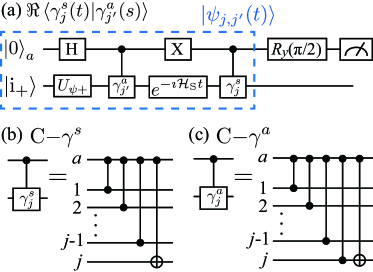
Figure 4: (a) QC algorithm of $\Re\braket{\gamma_{j}^{s}(t)}{\gamma_{j^{\prime}}^{a}(t)}$. $\ket{\mathrm{i}_{+}}$ denotes the initial state for even parity, corresponding to $\ket{0}^{\otimes N}$. The unitary gate of time evolution $e^{-\imath\mathcal{H}_{\mathrm{S}}t}$ is given by the Trotter decomposition whose circuit form is the same as $U_{\psi\pm}$, while the angles $\{\bm{\theta},\vartheta\}$ are set to constant by the model parameters $J_{\alpha}$, $h_{z}$, and infinitesimal time step $\Delta t$. (b,c) Control-$\gamma$ gates, consisting of CZ and CX gates.

IV.3 Quantum-circuit (QC) algorithm

In the finite-size systems, the MB winding number (30) are discretized as follows,

$$N_{w}=\frac{1}{2\pi}\sum_{k}\Im\log\left[Z_{k+\Delta k}Z_{k}^{\ast}\right],$$ (32)

with $\Delta k=2\pi/N$. Additionally, to determine the MB Anderson pseudo vector in the QC, we need to calculate the Green functions of MFs (31) in the real space,

$$Z_{k}=\frac{1}{2}g_{\gamma_{k}^{s},\gamma_{-k}^{a}}=\frac{1}{2N}\sum_{j,j^{\prime}}e^{-\imath(j-j^{\prime})k}g_{\gamma_{j}^{s},\gamma_{j^{\prime}}^{a}}.$$ (33)

To obtain the real-space Green function of MFs, we rewrite it by using the time-evolution form:

$$g_{\gamma_{j}^{s},\gamma_{j^{\prime}}^{a}} =2\Im\bra{\mathrm{gs}}\gamma_{j}^{s}\frac{1}{\mathcal{H}_{\mathrm{K}}-E_{\mathrm{gs}}}\gamma_{j^{\prime}}^{a}\ket{\mathrm{gs}}$$

$$=-\lim_{\delta\to+0}\lim_{T\to\infty}2\int_{0}^{T}\mathrm{d}t\,e^{-\delta t}\Re\braket{\gamma_{j}^{s}(t)}{\gamma_{j^{\prime}}^{a}(t)},$$ (34)

with two time-evolved MF-excited states,

$$\ket{\gamma_{j}^{s}(t)}=\gamma_{j}^{s}e^{-\imath\mathcal{H}_{\mathrm{K}}t}\ket{\mathrm{gs}},\ \ket{\gamma_{j}^{a}(t)}=e^{-\imath\mathcal{H}_{\mathrm{K}}t}\gamma_{j}^{a}\ket{\mathrm{gs}}.$$ (35)

Here, although we introduce the infinitesimal damping factor $\delta\to+0$ and the infinite cutoff time $T\to\infty$, these are set to be finite values in the numerical calculation. We should set the cutoff time $T$, satisfying $T\delta\gg 1$, with the small enough damping factor $\delta\ll 1$. The effects of finite values are important to obtain the winding number by using the Green-function matrix, whereas the effects are not clarified so far. Thus, the damping-factor dependence of $Z_{k}$ in the numerical calculations is discussed below.

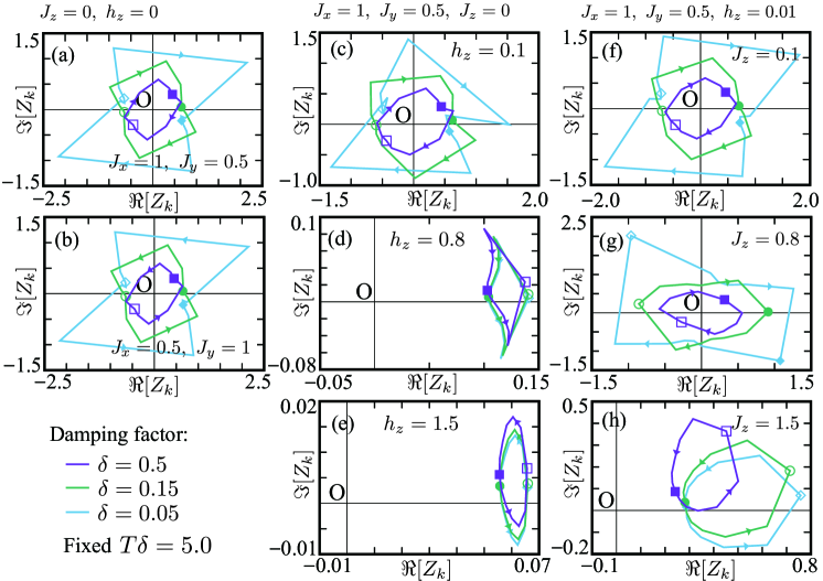
Figure 5: The MB Anderson pseudo vector $(\Re[Z_{k}],\Im[Z_{k}])$ obtained by the QC algorithm in Fig. 4 for the 12-site XYZ spin chain. Each panel shows $Z_{k}$ for the model-parameter point corresponding to Fig. 3. Namely, (a,b) left, (c-e) center, and (f-h) right panels show the XY anisotropy, the magnetic field, and the Ising term (i.e., the Coulomb interaction in the Kitaev chain) dependencies, respectively, with fixed other parameters. Purple, green, and cyan solid lines represent the damping factors $\delta=0.5$, $0.15$, and $0.05$, respectively, with fixed the cutoff time $T\delta=5$ and the Trotter time step $\Delta t=0.01$. Close (open) symbols denote $Z_{k=0}$ ($Z_{k=\pi}$), and arrows indicate the ascending order of $k$.

Besides, the real part of the transition amplitude corresponds to the expectation value of the $x$ component of Pauli matrix of an ancila qubit $\sigma_{a}^{x}$ as follows,

$$\Re\braket{\gamma_{j}^{s}(t)}{\gamma_{j^{\prime}}^{a}(t)}=\bra{\psi_{j,j^{\prime}}(t)}\sigma_{a}^{x}\ket{\psi_{j,j^{\prime}}(t)}$$ (36)

with

$$\ket{\psi_{j,j^{\prime}}(t)} =\frac{1}{\sqrt{2}}\left(\ket{1}_{a}\ket{\gamma_{j}^{s}(t)}+\ket{0}_{a}\ket{\gamma_{j^{\prime}}^{a}(t)}\right).$$ (37)

Therefore, we can calculate the expectation value in the QC given in Fig. 4(a). Note that a similar technique is proposed by Endo et al., to calculate the Green functions of fermions [70]. To implement the ground state, we use the even-parity initial state $\ket{\mathrm{i}_{+}}=\ket{0}^{\otimes N}$ and the wavefunction ansatz $U_{\psi+}$ in Fig. 2(e) with the optimized angles $\{\bm{\theta}_{j,m},\vartheta_{j,m}\}$ obtained by the VQE calculation. The MF operator $\gamma_{j}^{\tau}$ ($\tau=s,a$) can be introduced by a control unitary gate [see Fig. 4(b,c)]. The time evolution $e^{-\imath\mathcal{H}_{\mathrm{S}}t}$ in the QC algorithm for topological invariant [Fig. 4(a)] is given by the Trotter decomposition whose circuit form is the same as $U_{\psi\pm}$, while the angles $\{\bm{\theta},\vartheta\}$ are set to constant by the model parameters $J_{\alpha}$, $h_{z}$, and infinitesimal time step $\Delta t$,

$$\theta_{a}=\frac{J_{x}+J_{y}}{4}\Delta t,\ \theta_{b}=\frac{J_{x}-J_{y}}{4}\Delta t,\ \theta_{c}=\frac{J_{z}}{4}\Delta t,\ \vartheta=\frac{h_{z}}{2}\Delta t.$$ (38)

Figure 5 shows the MB Anderson pseudo vector $(\Re[Z_{k}],\Im[Z_{k}])$ obtained by the QC algorithm in Fig. 4, for various points in the model-parameter space of the 12-site XYZ spin chain, where the parameter points correspond to Fig. 3. The MB winding number is defined by the number of times that the MB Anderson pseudo vector $(\Re[Z_{k}],\Im[Z_{k}])$ circulates counterclockwise around the origin as well as the Anderson pseudo vector in the TB model. Colors of solid lines show different damping factors, $\delta=0.5$, $0.15$, and $0.05$, with fixed $T\delta=5$. Although the size and angle of $Z_{k}$ changes with changing the damping factor, the shape is roughly kept, and thus the winding number is conserved even if the damping factor is not so small. In addition, we have confirmed that the winding numbers are equal between the QC algorithm and the ED calculation. Consequently, our QC algorithm for the topological invariant can basically be applied to the current NISQ devices with the serious limitation of coherent time, although the error mitigation techniques are necessarily required.

V Majorana zero mode

In this section, we explain how to visualize the MZM. The MZM is a zero-energy excitation of MFs, localized at edges of chain [see Fig. 1]. We can understand the MZM if starting with the Majorana representation of the TB model, rewritten by

$$\mathcal{H}_{\mathrm{M}}|_{\zeta=0}=-\imath\bm{\gamma}_{s}^{T}\mathbf{H}_{\mathrm{M}}\bm{\gamma}_{a}$$ (39)

with the tridiagonal coefficient matrix

$$\mathbf{H}_{\mathrm{M}}=\begin{pmatrix}\eta&g_{-}&&&\\ g_{+}&\eta&g_{-}&&\\ &g_{+}&\eta&\ddots&\\ &&\ddots&\ddots&g_{-}\\ &&&g_{+}&\eta\end{pmatrix}$$ (40)

and the vector of MFs,

$$\bm{\gamma}_{\tau}=(\gamma_{1}^{\tau},\gamma_{2}^{\tau},\cdots,\gamma_{N}^{\tau})\hskip 10.00002pt(\tau=s,a).$$ (41)

Diagonalization of the matrix is obtained by the singular-value decomposition, resulting in $\mathbf{H}_{\mathrm{M}}=\mathbf{U}_{\mathrm{M}}\mathbf{\Lambda}_{\mathrm{M}}\mathbf{V}_{\mathrm{M}}^{\dagger}$, with the unitary matrices $\mathbf{U}_{\mathrm{M}}$ and $\mathbf{V}_{\mathrm{M}}$, and the diagonal matrix $\mathbf{\Lambda}_{\mathrm{M}}=\mathrm{diag}\{\lambda_{1},\lambda_{2},\cdots,\lambda_{N}\}$ with the ascending order singular values $\lambda_{l}<\lambda_{l+1}$. Then, the TB Majorana Hamiltonian (39) reads,

$$\mathcal{H}_{\mathrm{M}}|_{\zeta=0}=-\imath\sum_{l}\lambda_{l}\tilde{\gamma}_{l}^{s}\tilde{\gamma}_{l}^{a}$$ (42)

with the superposition of MFs,

$$\tilde{\gamma}_{l}^{s}=\sum_{j}(\mathbf{U}_{\mathrm{M}}^{\dagger})_{lj}\gamma_{j}^{s},\ \tilde{\gamma}_{l}^{a}=\sum_{j}(\mathbf{V}_{\mathrm{M}}^{\dagger})_{lj}\gamma_{j}^{a}.$$ (43)

Since the superposed MFs also have the anti-commutation relation $\{\tilde{\gamma}_{l}^{\tau},\tilde{\gamma}_{l^{\prime}}^{\tau^{\prime}}\}=2\delta_{l,l^{\prime}}\delta_{\tau,\tau^{\prime}}$ with the Hermiticy $(\gamma_{l}^{\tau})^{\dagger}=\gamma_{l}^{\tau}$ for $\tau(\tau^{\prime})=s,a$, we can put one fermion on two MFs, $\tilde{\gamma}_{l}^{s}=\tilde{c}_{l}^{\dagger}+\tilde{c}_{l}$ and $\tilde{\gamma}_{l}^{a}=\imath\left(\tilde{c}_{l}^{\dagger}-\tilde{c}_{l}\right)$. With these fermions, the TB Hamiltonian (42) is rewritten by,

$$\mathcal{H}_{\mathrm{M}}|_{\zeta=0}=-2\sum_{l}\lambda_{l}\left(\tilde{c}_{l}^{\dagger}\tilde{c}_{l}-\frac{1}{2}\right).$$ (44)

Therefore, the singular values are considered as the eigen-energies. If there is a zero singular value $\lambda_{1}=0$, the pair of MFs, $\tilde{\gamma}_{1}^{s}$ and $\tilde{\gamma}_{1}^{a}$, becomes the MZM.

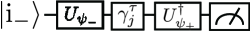
Figure 6: QC algorithm for the real-space distribution of the MZM, $|\bra{\mathrm{gs}_{+}}\gamma_{j}^{\tau}\ket{\mathrm{gs}_{-}}|$ for $\tau=s,a$. The probability to observe $\ket{0}^{\otimes N}$ corresponds to the transfer amplitude $|\bra{\mathrm{gs}_{+}}\gamma_{j}^{\tau}\ket{\mathrm{gs}_{-}}|$.

The on-site MFs $\gamma_{j}^{\tau}$ consist of creation and annihilation operators of fermion, so that single operation of the superposed MFs changes the fermion parity $\mathcal{F}$. Hence, the expectation value of the MFs for any parity-conserved eigenstates is always zero. Instead, to visualize the MZM, we need to see the transfer amplitude without finite energy excitation between different parity subspaces, e.g., the real-space distribution for symmetric mode reads

$$|\bra{\mathrm{gs}_{+}}\gamma_{j}^{s}\ket{\mathrm{gs}_{-}}|=\left|\sum_{l}(\mathbf{U}_{\mathrm{M}})_{jl}\bra{\mathrm{gs}_{+}}\tilde{\gamma}_{l}^{s}\ket{\mathrm{gs}_{-}}\right|=|(\mathbf{U}_{\mathrm{M}})_{j1}|,$$ (45)

because the transfer amplitude is zero except for $l=1$, namely, $|\bra{\mathrm{gs}_{+}}\tilde{\gamma}_{l}^{s}\ket{\mathrm{gs}_{-}}|=\delta_{l,1}$, if the first singular value is only zero, $\lambda_{1}=0$. Therefore, we can visualize the real-space distribution of the MZM by calculating the transfer amplitude, $|\bra{\mathrm{gs}_{+}}\gamma_{j}^{\tau}\ket{\mathrm{gs}_{-}}|$ for $\tau=s,a$ in the QC.

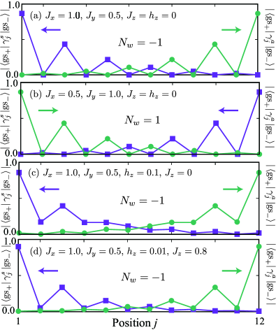
Figure 7: Visualization of the MZM in the 12-site XYZ spin chain by using the QC algorithm shown in Fig. 6 for various model-parameter points. The model parameters (a-d) correspond to (a), (b), (c), and (g) in Fig. 3 and Fig. 5.

Figure 7 shows the transfer amplitudes $|\bra{\mathrm{gs}_{+}}\gamma_{j}^{\tau}\ket{\mathrm{gs}_{-}}|$ in the topological state. The weight of MZM are localized at an edge and rapidly decreases with entering the bulk. Furthermore, we can see that the symmetric and antisymmetric modes switch the position if the winding number changes [compare (a) and (b) in Fig. 7]. The numerical cost of this QC algorithm for the MZM is much lower than that for topological invariant, so that it is easier to confirm the topological state with the MZM visualization. However, in this case, we should be careful with the energy difference between the ground states in even and odd parity subspaces, because there is usually an energy gap due to the finite-size effect.

VI Summary and Discussion

For realizing the long-term FTQC, topological states of matter are important, while the QC algorithms to determine topological invariant are still not sufficient. In this paper, we propose the QC algorithm for topological invariant by using time evolution. Since this algorithm requires the ground state with keeping the fermion parity, we also show the VQE method conserving the parity. In addition, we propose how to visualize the MZM in the QC, and demonstrate it on the QC simulator, qulacs [63], in the classical computer.

As the result of parity-conserved VQE calculations, we find that the ground states with odd parity are comparably difficult to be obtained. The non-uniform initial state before unitary operations in the QC may affect the convergence in the shallow QC. In the QC algorithm of topological invariant, we clarify that introducing the damping factor and the cutoff time only gives a slight change in the size and angle of the Anderson pseudo vector, but keeps the topological invariant. This feature guarantees the stability of our algorithms even with an inevitable noise in NISQ devices, while the shallow QC due to the short coherent time might make the topological character somewhat unstable. Then, to execute our algorithms in NISQ devices, combining with error mitigation techniques and long time evolution algorithms will be crucial. Alternatively, for the visualization of the MZM, our algorithm only requires the shallow QC, and thus, its demonstration is possible even in current NISQ devices.