$GW$ density matrix to estimate self-consistent $GW$ total energy in solids

Abstract

The $GW$ approximation is a well-established method for calculating ionization potentials and electron affinities in solids and molecules. For numerous years, obtaining self-consistent $GW$ total energies in solids has been a challenging objective that is not accomplished yet. However, it was shown recently that the linearized $GW$ density matrix permits a reliable prediction of the self-consistent $GW$ total energy for molecules [F. Bruneval et. al. J. Chem. Theory Comput. 17, 2126 (2021)] for which self-consistent $GW$ energies are available. Here we implement, test, and benchmark the linearized $GW$ density matrix for several solids. We focus on the total energy, lattice constant, and bulk modulus obtained from the $GW$ density matrix and compare our findings to more traditional results obtained within the random phase approximation (RPA). We conclude on the improved stability of the total energy obtained from the linearized $GW$ density matrix with respect to the mean-field starting point. We bring compelling clues that the RPA and the $GW$ density matrix total energies are certainly close to the self-consistent $GW$ total energy in solids if we use hybrid functionals with enriched exchange as a starting point.

I Introduction

While a few self-consistent $GW$ calculations (sc$GW$) for the band gaps of real solids are available [1, 2, 3], sc$GW$ total energies are still not available today, certainly because of their high computational cost. However, there exist hints that sc$GW$ could be accurate: first, the results on the homogeneous electron gas are extremely good [4, 5, 6]; second, the random-phase approximation (RPA) which derives from the same family has been shown to yield total energies capable of describing the tenuous van der Waals interactions [7, 8, 9, 10, 11, 12, 13]. Unfortunately, sc$GW$ calculations are very involved in real solids. That is why it would be highly desirable to obtain sc$GW$ quality energies without actually performing the cumbersome self-consistency.

Pursuing the quest for a non-self-consistent approximation to sc$GW$, a series of studies have been published in the early 2000s [14, 15, 16, 17, 18, 19]. More recently, some of us proposed an alternative non-self-consistent total energy expression based on the $GW$ density matrix, labeled $\gamma^{GW}$ [20, 21]. Benchmarks on small molecules for which sc$GW$ are possible [22, 23] confirmed the remarkable properties of the $\gamma^{GW}$ total energies: although it is evaluated non-self-consistently using a generalized Kohn-Sham (gKS) input, the resulting total energy remains quite insensitive to the gKS choice and approximates very well the reference sc$GW$ total energies.

In this context, this study focuses on the evaluation of total energies in solids. We port to the solid systems the $\gamma^{GW}$ total energy with the sensible prospect that it will remain a good approximation to the sc$GW$ total energy. In doing so, we obtain the correlated density matrix $\gamma^{GW}$ as a physically meaningful intermediate object with unique properties due to correlation.

When considering solid systems several technical questions have to be addressed. Firstly, the closed formulas obtained for finite systems [24, 20] have to be adapted for numerical efficiency. Secondly, the pseudopotentials [25] that are customary in the plane-wave basis codes are typically designed to be used in conjunction with standard semi-local approximations to density-functional theory. Therefore, it is necessary to investigate which type of pseudopotential is suitable for obtaining consistently $GW$-type total energies.

With this, we will study the performance of the $\gamma^{GW}$ total energy for solids. We will compare it to the popular RPA total energy which may be derived as the $GW$ approximation of the Klein functional [26, 27, 14]. As all these calculations are performed as a one-shot procedure, memory about the mean-field starting point is present. We will particularly investigate this issue by varying the content of exact exchange $\alpha$ in the hybrid functional PBEh($\alpha$), zero being the standard PBE [28] and 0.25 yielding regular PBE0 [29]. It is therefore always necessary to specify the exact procedure used to obtain a one-shot energy. We do so here using the @ notation (e.g. RPA@PBE stands for the RPA total energy evaluated with self-consistent PBE inputs).

The article is organized as follows: In Sec. II, we recapitulate the theoretical foundation for the $GW$ density matrix and derive the working equations; In Sec. III, we detail the technical aspects of the implementation in a plane-wave code and assess the pseudopotential choice; Sec. IV shows some of the unique properties of the $GW$ density matrix, exemplified with bulk silicon; In Sec. V, we benchmark the total energies obtained with the different approximations with a test set of 7 standard covalent semiconductors and one layered material. Finally, Sec. VI concludes our work.

II Theory and working formulas

II.1 Green’s function-derived density matrix

In the many-body perturbation theory, the central quantity, namely the one-particle Green’s function $G(\mathbf{r},\mathbf{r}^{\prime},\omega)$, contains a great deal of information. In particular, by virtue of the Galistkii-Midgal formula [30], it is sufficient to calculate the total energy of an electronic system.

Also it straightforwardly yields the density matrix $\gamma(\mathbf{r},\mathbf{r}^{\prime})$

$$\gamma(\mathbf{r},\mathbf{r}^{\prime})=-\frac{\mathrm{i}}{2\pi}\int_{-\infty}^{+\infty}d\omega e^{i\eta\omega}G(\mathbf{r},\mathbf{r}^{\prime},\omega),$$ (1)

where $\eta$ is a vanishing positive real number that enforces the sensitivity to the occupied manifold of the time-ordered Green’s function $G$. Hence, the electronic density can be obtained as the diagonal: $\rho(\mathbf{r})=\gamma(\mathbf{r},\mathbf{r})$.

Therefore, the Green’s function methods, such as the $GW$ approximation, can give access to an approximate density matrix.

II.2 Linearized Dyson equation

In the many-body perturbation theory, the overall strategy is to connect the exact Green’s function $G$ to a known Green’s function $G_{0}$. The connection between the two is ensured by the complicated self-energy $\Sigma_{xc}$ that is in charge of all the correlation effects.

The expression of $G_{0}$ that is derived from a mean-field approach (Kohn-Sham, Hartree-Fock, etc.), is simple:

$$G_{0}(\mathbf{r},\mathbf{r}^{\prime},\omega)=2\sum_{\mathbf{k}i}\frac{\varphi_{\mathbf{k}i}(\mathbf{r})\varphi_{\mathbf{k}i}^{*}(\mathbf{r}^{\prime})}{\omega-\epsilon_{\mathbf{k}i}\pm\mathrm{i}\eta},$$ (2)

where $\varphi_{\mathbf{k}i}(\mathbf{r})$ and $\epsilon_{\mathbf{k}i}$ are the mean-field wavefunctions and eigenvalue for state $i$ at k-point $\mathbf{k}$ and the small positive $\eta$ ensures the correct location of the poles for a time-ordered function (above the real axis for occupied states $\epsilon_{\mathbf{k}i}<\mu$ and below the real axis for empty states $\epsilon_{\mathbf{k}i}>\mu$, $\mu$ being the Fermi level). Spin-restricted calculations are assumed here and the factor 2 accounts for it.

Then the connection from $G_{0}$ to $G$ is made with the so-called Dyson equation:

$$G=G_{0}+G_{0}(\Sigma_{xc}-V_{xc})G,$$ (3)

where $V_{xc}$ is the exchange-correlation operator (possibly including non-local exchange) the space and frequency indices have been omitted for conciseness.

The self-energy $\Sigma_{xc}$ is itself a functional of the exact $G$. When approximating $\Sigma_{xc}$ and $G$, only a self-consistent solution ensures the conservation of the electron count [31]. In particular, for the $GW$ approximation of $\Sigma_{xc}$ that is most often evaluated with a one-shot procedure, the violation of electron conservation is well documented [32, 18, 33, 21].

In a previous study of ours [21], it was demonstrated analytically and verified numerically that linearizing the Dyson equation completely cures the problem of electron count conservation in the $GW$ approximation. The linearized Dyson equation (LDE) reads

$$G=G_{0}+G_{0}(\Sigma_{xc}-V_{xc})G_{0},$$ (4)

where the last $G$ in Eq. (3) had been simply replaced by $G_{0}$. The LDE is customary in the context of the Sham-Schüter equation [34].

This electron-conserving equation is then applied with the $GW$ approximation to $\Sigma_{xc}$.

II.3 $GW$ self-energy based density matrix

The $GW$ approximation [35] is simply sketched here, since it has been the subject of numerous detailed reviews [36, 37, 38].

The screened Coulomb interaction $W$ is defined with the Dyson-like equation:

$$W=v+v\chi_{0}W,$$ (5)

where $\chi_{0}=-2\mathrm{i}GG$ is the non-interacting polarizability and $v$ is the usual bare Coulomb interaction.

The $GW$ self-energy then reads

$$\Sigma_{xc}=\mathrm{i}GW.$$ (6)

It is convenient to decompose the self-energy into pure exchange and correlation. The exchange part $\Sigma_{x}$ is static, whereas the correlation part carries the frequency dependence $\Sigma_{c}(\omega)$. These quantities are routinely obtained with a one-shot procedure in standard periodic codes [39, 40]

Some general properties of the density matrix are detailed in App. A. For instance, it is demonstrated that the density matrix can be fully characterized with a single k-point index within the first Brillouin zone, even though it is a function of two spatial indices.

Now let us focus on the $GW$ density matrix. It is handy to project into the mean-field orbitals $|\mathbf{k}i\rangle$, which form a valid orthogonal basis:

$$\gamma_{\mathbf{k}ij} = \langle\mathbf{k}i|\gamma|\mathbf{k}j\rangle$$ (7)

$$= \int d\mathbf{r}d\mathbf{r}^{\prime}\varphi_{\mathbf{k}i}^{*}(\mathbf{r})\gamma(\mathbf{r},\mathbf{r}^{\prime})\varphi_{\mathbf{k}j}(\mathbf{r}^{\prime}).$$

The first term on the right-hand side of Eq. (4) is $G_{0}$. Let us insert it in Eq. (1) and project on the orbital basis to obtain the spin-summed density matrix elements

$$\gamma^{\mathrm{gKS}}_{\mathbf{k}ij}=2\delta_{ij}\theta(\mu-\epsilon_{\mathbf{k}i}).$$ (8)

This expression has been obtained by closing the contour in the upper part of the complex plane so that only the poles located above the real axis have survived.

A similar approach technique can be used for the static terms in the right-hand part of Eq. (4), $G_{0}(\Sigma_{x}-V_{xc})G_{0}$:

$$\Delta\gamma^{\mathrm{HF}}_{\mathbf{k}ij}=2\theta(\mu-\epsilon_{\mathbf{k}i})\theta(\epsilon_{\mathbf{k}j}-\mu)\frac{\langle\mathbf{k}i|\Sigma_{x}-V_{xc}|\mathbf{k}j\rangle}{\epsilon_{\mathbf{k}i}-\epsilon_{\mathbf{k}j}}.$$ (9)

We denote it with a “HF” superscript because this contribution to the (spin-summed) linearized density matrix is obtained from a pure exchange self-energy; thus, it vanishes when the HF approximation is employed to obtain the mean-field orbitals (i.e. $\Delta\gamma^{\mathrm{HF}}=0$ for $\gamma^{\mathrm{gKS}}=\gamma^{\mathrm{HF}}$).

For the last term in Eq. (4), $G_{0}\Sigma_{c}G_{0}$, the self-energy $\Sigma_{c}$ has a frequency dependence and therefore the calculations cannot be performed analytically in contrast with the two previous terms, it is convenient to perform the integration along the imaginary axis, so as to keep some distance with the poles of $G_{0}$ and of $\Sigma_{c}$. Closing the contour, we transform the real-axis integration of Eq. (1) into

$$\Delta\gamma^{GW}_{\mathbf{k}ij}=\frac{1}{\pi}\int_{-\infty}^{+\infty}d\omega\frac{\langle\mathbf{k}i|\Sigma_{c}(\mu+\mathrm{i}\omega)|\mathbf{k}j\rangle}{(\mu+\mathrm{i}\omega-\epsilon_{\mathbf{k}i})(\mu+\mathrm{i}\omega-\epsilon_{\mathbf{k}j})}.$$ (10)

The complete spin-summed linearized $GW$ density matrix finally reads

$$\gamma^{GW}=\gamma^{\mathrm{gKS}}+\Delta\gamma^{\mathrm{HF}}+\Delta\gamma^{GW}.$$ (11)

Lastly, the corresponding electronic density is $\rho^{GW}(\mathbf{r})=\gamma^{GW}(\mathbf{r},\mathbf{r})$.

II.4 Total energies from $GW$ density matrix

In previous studies [20, 21], we introduced a new total energy functional:

$$E_{\mathrm{total}}^{\gamma^{GW}}=T[\gamma^{GW}]+V_{ne}[\rho^{GW}]+E_{H}[\rho^{GW}]\\ +E_{x}[\gamma^{GW}]+E_{c}[G_{0}]+V_{nn},$$ (12)

where $T$, the kinetic energy, $V_{ne}$, the electron-nucleus interaction, $E_{H}$, the Hartree energy, $E_{x}$ the exchange energy are evaluated with $\gamma^{GW}$ density matrix. Klimes et. al. [41] also used the $GW$ (or RPA) density matrix to improve sub-parts of the energy. Just the correlation energy $E_{c}$ cannot be calculated with $\gamma^{GW}$ and is pragmatically obtained from the Galitskii-Migdal equation [21]:

$$E_{c}[G_{0}]=\frac{1}{4\pi}\int_{-\infty}^{+\infty}d\omega\mathrm{Tr}\{v\chi_{0}(i\omega)-v\chi(i\omega)\},$$ (13)

where $\chi=\chi_{0}+\chi_{0}v\chi$ is the RPA polarizability.

This one-shot energy expression has the desirable property that all the input quantities conserve the number of electrons. Of course, being a one-shot total energy, it keeps a dependence with respect to the starting point. This will be studied in detail in Sec. V.

II.5 RPA total energy

For completeness, we report here without derivation the RPA expression for the total energy as we will extensively compare $E_{\mathrm{total}}^{\mathrm{RPA}}$ and $E_{\mathrm{total}}^{\gamma^{GW}}$ in the following.

The RPA correlation is defined as [42]

$$\Phi_{c}[G_{0}]=\frac{1}{4\pi}\int_{-\infty}^{+\infty}d\omega\,\mathrm{Tr}\left\{v\chi_{0}(i\omega)+\mathrm{ln}\left[1-v\chi_{0}(i\omega)\right]\right\}.$$ (14)

By construction, $\Phi_{c}[G_{0}]$ contains the correlation part of the kinetic energy. The total one-shot energy expression reads

$$E_{\mathrm{total}}^{\mathrm{RPA}}=T[\gamma^{\mathrm{gKS}}]+V_{ne}[\rho^{\mathrm{gKS}}]+E_{H}[\rho^{\mathrm{gKS}}]\\ +E_{x}[\gamma^{\mathrm{gKS}}]+\Phi_{c}[G_{0}]+V_{nn}.$$ (15)

The one-shot RPA total energy is known to have a noticeable starting point dependence [15, 43, 44, 21]. We will quantify this in Sec. V in comparison with $E_{\mathrm{total}}^{\gamma^{GW}}$.

III Implementation and computational details

The linearized $GW$ density matrix in periodic systems has not been studied before to the best of our knowledge. It should be noted though that the linearized $GW$ density matrix appears as an intermediate quantity in the RPA forces derived by Ramberger et al. [45].

In this section, we provide a detailed description of our implementation of $\gamma^{GW}$ in the ABINIT code [40]. We also highlight the key technical aspects that are crucial for producing accurate results.

III.1 Implementation in a periodic plane-wave approach

ABINIT is a standard plane-wave-based DFT code. The core electrons are frozen and hidden in a pseudopotential. While the Kohn-Sham part of ABINIT is able to use the more accurate and smoother projector augmented-wave atomic datasets [46, 47, 48], the extension to $GW$ is very delicate [49, 50]. As of today, the $GW$ part of ABINIT is fully validated only for regular norm-conserving pseudopotentials [51, 52].

The existing implementation in ABINIT provides us with $\langle\mathbf{k}i|\Sigma_{c}(\mu+\mathrm{i}\omega)|\mathbf{k}j\rangle$ for any value of $\omega$. From this starting point, we have then implemented a Gauss-Legendre quadrature to perform the integral in Eq. (10). The symmetry relation

$$\langle\mathbf{k}i|\Sigma_{c}(\mu-\mathrm{i}\omega)|\mathbf{k}j\rangle=\langle\mathbf{k}j|\Sigma_{c}(\mu+\mathrm{i}\omega)|\mathbf{k}i\rangle^{*}$$ (16)

is employed to limit the integration from 0 to $+\infty$. A grid with typically 50 to 120 grid points is sufficient to ensure a very accurate convergence: we monitor the electron count deviation, which is always kept below $10^{-3}$. In the future, grid design could be optimized to minimize the computational burden [33, 53].

The static term from Eq. (9) has been implemented as well, for any type of exchange-correlation potential $V_{xc}$, including those based on hybrid functionals. Note that for a Hartree-Fock mean-field starting point, the static term $\Sigma_{x}-V_{xc}$ vanishes. Furthermore, it is clear from Eq. (9) that the linearized density matrix is limited to systems with a finite band gap, or else diverging denominators would occur.

The matrix representation of $\gamma^{GW}$ is obtained on the gKS states $|\mathbf{k}i\rangle$ for $i\leq N_{b}$. We then diagonalize it to obtain the natural orbitals in the gKS basis:

$$\sum_{j=1}^{N_{b}}\gamma_{\mathbf{k}ij}U_{\mathbf{k}j\lambda}=n_{\mathbf{k}\lambda}U_{\mathbf{k}i\lambda},$$ (17)

where $n_{\mathbf{k}\lambda}$, the eigenvalues, are the so-called natural occupations and where $U_{\mathbf{k}j\lambda}$, the eigenvector coefficients, form the natural orbitals.

In other words, the natural orbitals $\phi_{\mathbf{k}\lambda}(\mathbf{r})=\langle\mathbf{r}|\mathbf{k}\lambda\rangle$ can be obtained from the unitary matrix $U_{\mathbf{k}i\lambda}$:

$$\phi_{\mathbf{k}\lambda}(\mathbf{r})=\sum_{i=1}^{N_{b}}U_{\mathbf{k}i\lambda}\varphi_{\mathbf{k}i}(\mathbf{r}).$$ (18)

Then all the one-body operators expectation values are readily obtained. For instance, the kinetic energy $T$ is calculated as

$$T =\frac{1}{N_{k}}\sum_{\mathbf{k}\lambda}n_{\mathbf{k}\lambda}\langle\mathbf{k}\lambda|\hat{T}|\mathbf{k}\lambda\rangle$$ (19)

$$=\frac{1}{N_{k}}\sum_{\mathbf{k}\lambda}n_{\mathbf{k}\lambda}\sum_{ij}U_{\mathbf{k}i\lambda}^{*}U_{\mathbf{k}j\lambda}\langle\mathbf{k}i|\hat{T}|\mathbf{k}j\rangle.$$ (20)

Finally, we would like to emphasize that the formal proof of the conservation of electron count [21] requires that the state range in the internal sum of $G_{0}$ in Eq. (2) is the same as the one used in the basis expansion in Eq. (7). This restriction is enforced in all our calculations.

Table 1 summarizes the numerical parameters used for the 8 crystals considered in this study. All the calculations for face-centered cubic crystals reported in this work use four shifted k-point grids, as commonly used in ABINIT. The grid discretization is $4\times 4\times 4$, which yields 256 k-points in the full Brillouin zone and 10 in the irreducible wedge. The calculation on hexagonal boron nitride (h-BN) uses a $\Gamma$-centered $12\times 12\times 6$ k-point grid for exact exchange and a $4\times 4\times 2$ grid for the rest. We evaluate the computational effort to scale as $O(N^{4})$, similar to a conventional $GW$ calculation. However, the prefactor is much larger, due to the fine frequency grids for both $W$ and $\Sigma$.

Table 1: Energy cutoff for the wavefunctions ($E_{cut}^{\varphi}$, in Hartree), energy cutoff for the plane-waves expansion of the screened Coulomb interaction $W$ ($E_{cut}^{W}$, in Hartree), number of bands ($N_{b}$) in $G_{0}$ and in Eqs. (9,10), number of pure imaginary frequencies ($N_{\omega_{W}}$) used for $W(\mathrm{i}\omega)$, and number of frequency points ($N_{\omega_{\Sigma}}$), used for the quadrature along the imaginary axis in Eq. (10).

	Si	C	SiC	zb-BN	AlP	AlAs	Ge	h-BN
$E_{cut}^{\varphi}$	12	25	50	40	35	35	30	55
$E_{cut}^{W}$	8	15	15	15	15	10	10	25
$N_{b}$	150	175	175	175	175	175	175	1400
$N_{\omega_{W}}$	120	120	120	120	120	120	120	40
$N_{\omega_{\Sigma}}$	60	60	60	60	60	60	60	—

III.2 Adequate norm-conserving pseudopotentials

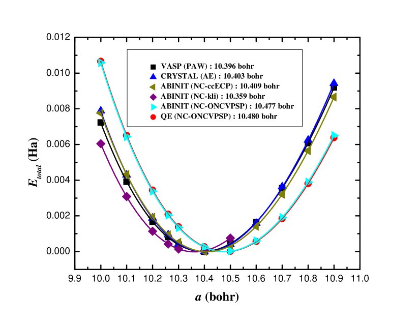
Figure 1: HF total energies as a function of lattice constant with different codes and pseudopotentials for bulk silicon. The equilibrium lattice constant for each calculation is given in the legend.

As mentioned in the previous paragraph, our implementation uses norm-conserving pseudopotentials. In the preliminary stages of our study, we concluded that while the details of the pseudopotential are not critical when studying band structures, they become of the utmost importance when investigating structural properties.

Norm-conserving pseudopotentials are designed to reproduce the electronic and energetic properties of a given mean-field approximation. For instance, using a PBE pseudopotential for a hybrid functional is not advised in principle. As no “$GW$-suitable” pseudopotentials exist, we have enforced the minimal requirement that the selected pseudopotential be able to reproduce HF structural properties.

In Fig. 1, we show a wide comparison among codes and techniques for bulk silicon at the HF level of theory. Silicon is chosen as a typical example. The results for two other crystals are reported in the supporting information with identical conclusions. The all-electron (AE) of CRYSTAL[54] with the accurate basis set designed by Heyd and coworkers [55] and the projector augmented-wave (PAW) results of VASP [39] agree very well. We consider them as the reference, since by construction, the Gaussian basis set used in CRYSTAL describes all the electrons at once and since in the PAW framework, though frozen-core, the core-valence interactions are completely recalculated for each approximation.

Then we turn to the regular PBE pseudopotential obtained from the pseudodojo suite [56]. This pseudopotential is highly tested and should be rather transferable as it relies on Hamann’s ONCVPSP scheme [52] that introduce several projectors per angular momentum. However, based on Fig. 1, the HF energy-volume curve departs significantly from the reference. This error is intrinsic to the pseudopotential because using it in Quantum-Espresso [57] gives the exact same result. In our opinion, the inability of the ONCVPSP pseudopotentials to reproduce HF energy-volume curves is not due to the Hamann’s scheme itself, but rather due to the practical choice of large cutoff radii selected in the pseudodojo initiative. Generating our own dedicated ONCVPSP pseudopotentials would be possible of course, however, would require a significant effort. Fortunately, alternatives already exist.

In a previous work [13], one of us mitigated this problem by using pseudopotentials generated for KLI[58] which devises a local potential that simulates the non-local exact-exchange operator. This improves over the ONCVPSP pseudopotentials but is not quantitative enough.

Recently, in the quantum Monte Carlo community, there has been an effort to support the design of “correlation consistent” effective core potentials (ccECP) [59]. These norm-conserving pseudopotentials are meant to be used in combination with correlated methods beyond the usual mean-field ones. Figure 1 shows that this type of pseudopotential produces results in close agreement with AE and PAW for HF: the lattice constants match within 0.1 %.

We conclude that the ccECP pseudopotentials are our preferred norm-conserving pseudopotentials to obtain quantitative results: i) they have been designed specifically for explicit-correlation methods and $GW$ belongs to this family; ii) they are best to reproduce HF lattice constants. The main drawback of these pseudopotentials is the high cutoff energy that is necessary to converge the total energies in plane waves. In the following, all the reported results employ ccECP pseudopotentials.

IV $GW$-density matrix in crystalline solids

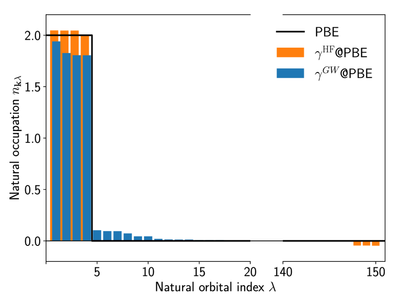
Figure 2: Spin-summed natural occupations obtained from PBE, $\gamma^{\mathrm{HF}}$@PBE, and $\gamma^{GW}$@PBE density-matrices in bulk silicon for k-point (1/8, 0, 0) in reciprocal lattice vectors. The natural occupations are ordered by descending values, from 1 to 150, which is $N_{b}$, the dimension of the matrix. The x-axis has been cut to show the first and the last values.

As summarized in Appendix A, the spin-summed natural occupations $n_{\mathbf{k}\lambda}$ should continuously span the range from 0 to 2 at variance with regular Fermi-Dirac ground-state occupations $f_{\mathbf{k}i}$ that are only 0 or 2.

These natural occupations for realistic crystalline solids can be compared to the momentum distribution function $n_{\mathbf{k}}$ for the homogeneous electron gas in Refs. [36, 60]. But for the homogeneous electron gas, the momentum $\mathbf{k}$ is enough to uniquely characterize the quantum state. For solids, we need an additional quantum number $\lambda$ (similar to a band index).

In Fig. 2, we represent the natural occupations $n_{\mathbf{k}\lambda}$ for a fixed k-point (1/8, 0, 0). This particular k-point was selected as an example: the other k-points produce very similar results. The PBE occupations $f_{\mathbf{k}i}$ are shown as a reference. Then the natural occupations for $\gamma^{\mathrm{HF}}$@PBE, the static part of the density matrix, are plotted. While their sum precisely equalizes the number of electrons $N_{e}$, the values can exceed 2 and be below 0. These occupation values violate the constraints of the exact density matrix. However, after adding the dynamic correlation, the $\gamma^{GW}$@PBE has all its spin-summed natural occupations between 0 and 2. Four natural orbitals have an occupation close to 1.8-1.9 and then many more (15 or so) have a non-vanishing occupation. A PBE mean-field starting point was chosen to magnify the effect. Starting from HF would yield perfectly sane natural occupations for $\gamma^{\mathrm{HF}}$ The overall shape of the occupation is similar to the homogeneous electron gas result [36, 60].

However one notices that $N(\mathbf{k})=\sum_{\lambda}n_{\mathbf{k}\lambda}$ for a given $\mathbf{k}$ slightly deviates from the number of electrons $N_{e}$. This intriguing observation does not violate an exact constraint. We only proved mathematically [21] that the sum of the natural occupation over the whole Brillouin zone

$$\sum_{\mathbf{k}}\sum_{\lambda}n_{\mathbf{k}\lambda}=N_{e}$$ (21)

is valid. Appendix B demonstrates that this variation with $\mathbf{k}$ is possible.

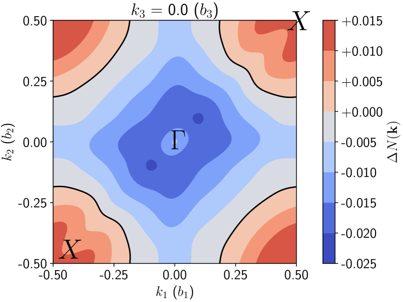
Figure 3: Electron count deviation $\Delta N(\mathbf{k})$ as a function of the wavevector $\mathbf{k}$ in the first Brillouin zone for bulk silicon. $\mathbf{k}=k_{1}\mathbf{b}_{1}+k_{2}\mathbf{b}_{2}+k_{3}\mathbf{b}_{3}$ is reported in reduced coordinates ($\mathbf{b}_{i}$ are the reciprocal lattice vectors). The plane $k_{3}=0$ is represented. The isoline $\Delta N(\mathbf{k})=0$ is drawn with a bold black line. Special points $\Gamma$ and $X$ are marked.

As this observation can be considered surprising when compared to the usual mean-field occupations $f_{\mathbf{k}i}$, it is insightful to monitor the sum $N(\mathbf{k})$ across the Brillouin zone. In Fig. 3, we report the deviation $\Delta N(\mathbf{k})=N(\mathbf{k})-N_{e}$ in a cut plane in the Brillouin zone. The $\Delta N(\mathbf{k})$ function is interpolated from a refined $\Gamma$-centered $6\times 6\times 6$ with 4 shifts k-point grid (864 points in the full Brillouin zone). We use the Shankland-Koelling-Wood interpolation technique [61] as implemented in abipy [40]. The numerical integration of $\Delta N(\mathbf{k})$ over the whole Brillouin yields $4\times 10^{-4}$, which is very close to the expected zero.

From Fig. 3, we observe an electron transfer from the $\Gamma$ point region to the Brillouin zone edge. The weight transfer is not large (at most $\sim 0.01-0.02$), but still sizable. The electron count $N(\mathbf{k})$ is an observable and could be possibly measured in angle-resolved photo-emission spectroscopy [62]. Note that this electron count transfer is a pure electronic correlation effect. Any static approximation of the self-energy $\Sigma$ would nullify it.

V Structural properties of crystalline solids within $GW$ density matrix and RPA

V.1 Covalent-bonded crystals

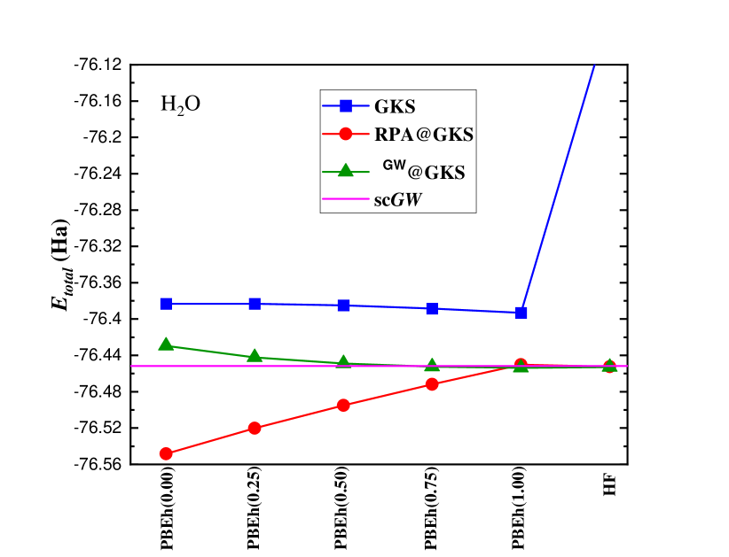
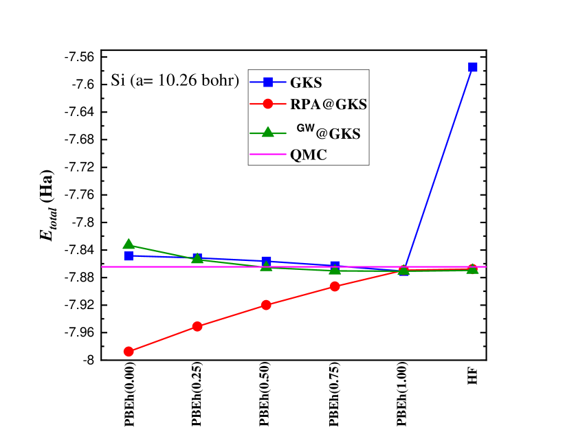
Figure 4: Total energies for the water molecule in the gas phase (left-hand panel) and crystalline silicon (right-hand panel) as a function of the gKS starting point. The water results were extracted from a previous study [21]. The silicon Quantum Monte Carlo (QMC) value comes from Ref. 63.

In this section, we analyze the calculation of structural parameters for crystalline solids using the total energy expressions introduced in Eqs. (12) and (15). Our main question is which expression works “best” in the context of one-shot calculations, i.e. which expression best approximates a hypothetical reference sc$GW$ that is not currently available for crystalline systems. In molecules, where reference sc$GW$ were produced [21], the accuracy of the $\gamma^{GW}$ total energy was demonstrated.

A way to measure the robustness of a one-shot total energy expression is to explore its sensitivity to the starting point. Here we use the PBEh($\alpha$) hybrid functional family:

$$V_{xc}=\alpha\Sigma_{x}+(1-\alpha)v_{x}^{\mathrm{PBE}}+v_{c}^{\mathrm{PBE}},$$ (22)

where the parameter $\alpha$ controls the amount of exact-exchange $\Sigma_{x}$.

Calculations were carried out for seven covalent crystals (Si, C, SiC, zb-BN, AlP, AlAs, and Ge). In the main text, we will mostly report silicon results. However, the complete set of results is made available as Supplemental Material [64].

In Fig. 4, we compare the total energy behavior for 2 different systems: water, a small molecular system, and crystalline silicon. The results for the water molecule were extracted from Ref. 21 that was using a different implementation based on Gaussian basis [65]. The figure reports the total energies for PBEh($\alpha$), for $E_{\mathrm{total}}^{\gamma^{GW}}$, for $E_{\mathrm{total}}^{\mathrm{RPA}}$, and when available for sc$GW$. The overall similarity between the two panels is striking: RPA is rather sensitive to the starting gKS, whereas $\gamma^{GW}$ is much less so. RPA increases with $\alpha$, whereas $\gamma^{GW}$ decreases. RPA and $\gamma^{GW}$ rejoin for large values of $\alpha$.

For water, where the sc$GW$ reference exists, the RPA and $\gamma^{GW}$ total energies give the best approximation of the full sc$GW$ total energy when they are equal. Owing to the similarity between the two panels of Fig. 4, we can reasonably anticipate that in bulk silicon, the sc$GW$ total energy will be best approximated by $\gamma^{GW}$ and by RPA with PBEh(0.75), PBEh(1.00) or HF, however with no formal proof.

If supplied with the sc$GW$ Green’s function, all total energy formulas should match [14, 15, 19]. The above results tend to make us think that the non-interacting Green’s function $G_{0}$ for PBEh(0.75), PBEh(1.00), or HF are close to the sc$GW$ Green’s function $G$ for both the molecular and the solid-state systems.

The striking difference between the molecule and the solid in Fig. 4 is the agreement or the disagreement with respect to the gKS total energies. While for the molecule, the RPA and the $\gamma^{GW}$ were undershooting much the total energy with respect to PBEh($\alpha$) (too negative correlation energies), the match is very good for crystalline silicon. The accurate quantum Monte Carlo approach reports -7.8644 Ha for silicon [63], whereas $\gamma^{GW}$ and RPA respectively give -7.8708 and -7.8692 Ha with the same ccECP pseudopotentials. This excellent agreement of the absolute total energies reminds us about the amazingly accurate sc$GW$ energies in the homogeneous electron gas [4, 5, 6] that precisely match the quantum Monte Carlo values [66].

We conclude with some reasonable confidence that the sc$GW$ total energy in bulk silicon is certainly close to the gKS, close to $E_{\mathrm{total}}^{\gamma^{GW}}$, and close to RPA@PBEh(1.00). We also stress that RPA@PBE, which is the most commonly accepted implementation of RPA functional, underestimates noticeably the total energy. Our confidence in these results is further strengthened when considering the results for the other 6 crystalline systems reported in the Supplemental Material [64]. They all support the same conclusion.

However if sc$GW$ is very accurate for solids and less accurate for finite systems, the atomization energies that measure the energy gain when forming a bulk crystal as compared to the isolated atoms are likely to have a low accuracy in sc$GW$. This should be explored in the future.

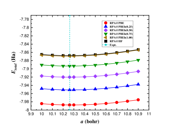
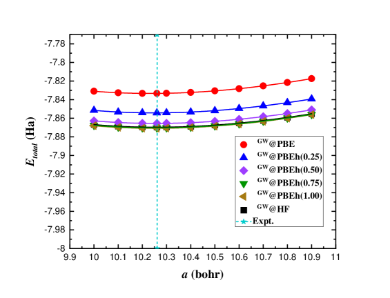
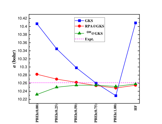
Figure 5: Energy-lattice constant curves for crystalline silicon for RPA functional (left-hand panel), $\gamma^{GW}$ energy functional (central panel). Equilibrium lattices are summarized in the right-hand panel. The experimental lattice constant is given as a reference.

Let us now focus on the complete energy versus lattice constant curves and check the sensitivity to the starting point not only for the total energy but also for the equilibrium lattice constant $a$ and for the bulk modulus $B$.

Figure 5 reports on the same scale the RPA and the $\gamma^{GW}$ total energies for different gKS starting points and in the right-hand panel the equilibrium lattice constant as a function of the gKS starting point. We can see again that the RPA total energy in the left-hand panel of Fig. 5 is much more sensitive to the starting point compared to $\gamma^{GW}$ total energy in the central panel. However, when focusing on the equilibrium lattice constant itself, the sensitivity to the starting point is much weaker: at most 0.03 bohr.

All panels in Fig. 5 support again the same conclusion: the RPA and $\gamma^{GW}$ total energies agree best when using PBEh($\alpha$) with large $\alpha$ or even when using HF. The statements drawn for silicon perfectly hold for the other 6 crystalline systems presented in the Supplemental Material [64].

Table 2: Lattice constants $a$ (bohr), bulk moduli $B$ (GPa), mean absolute error (MAE), and mean absolute percentage error (MAPE) of 7 covalent crystals obtained with several total energy methods.

		Si	C	SiC	zb-BN	AlP	AlAs	Ge	MAE	MAPE
PBEh(0.00)	$a$	10.407	6.774	8.310	6.861	10.471	10.847	10.947	0.101	1.00
	$B$	88.44	441.76	216.68	380.18	82.72	69.98	62.24	21.961	10.5
RPA@PBEh(0.00)	$a$	10.282	6.815	8.257	6.867	10.308	10.725	10.769	0.011	0.12
	$B$	97.08	477.44	235.25	401.35	96.78	83.57	86.10	12.123	8.7
$\gamma^{GW}$@PBEh(0.00)	$a$	10.232	6.713	8.180	6.800	10.287	10.668	10.708	0.011	0.12
	$B$	104.58	420.75	262.57	417.06	101.56	87.73	85.70	11.451	8.3
PBEh(0.75)	$a$	10.260	6.675	8.170	6.728	10.322	10.680	10.682	0.036	0.49
	$B$	111.93	502.28	270.10	461.11	102.44	88.02	87.30	31.026	15.7
RPA@PBEh(0.75)	$a$	10.254	6.759	8.210	6.831	10.301	10.683	10.738	0.012	0.13
	$B$	103.37	438.89	252.60	408.86	99.96	85.94	81.01	10.407	7.8
$\gamma^{GW}$@PBEh(0.75)	$a$	10.255	6.748	8.207	6.825	10.301	10.681	10.732	0.010	0.11
	$B$	103.91	436.08	254.39	410.23	100.22	86.59	82.07	11.619	8.4
Expt.	$a$	10.261	6.741	8.213	6.833	10.301	10.675	10.692	—	—
	$B$	99	443	225	369-400	86	77	76	—	—

Finally, we summarize the lattice constants and bulk moduli of the 7 covalent crystals that we have studied in Table 2. We focus on two gKS starting points PBEh(0.00) (i.e. standard PBE) and PBEh(0.75). While for PBE starting point the RPA@PBE and $\gamma^{GW}$@PBE lattice constants differ by about 0.06 bohr, the RPA@PBEh(0.75) and $\gamma^{GW}$@PBEh(0.75) lattice constants always agree within 0.01 bohr. The same type of conclusion holds for the bulk modulus $B$. This is another proof that PBEh(0.75) is a good starting point to evaluate the different $GW$-based total energy expressions. Most probably, the properties $a$ and $B$ evaluated with RPA@PBEh(0.75) or $\gamma^{GW}$@PBEh(0.75) are reliable estimates to the sc$GW$ result.

In the end, we also compare to experiment. Table 2 shows that all the $GW$-based energy expressions yield structural properties in excellent agreement with respect to the experiment: a 0.1 % deviation for lattice constants and 8 % for bulk moduli. The different expressions and starting points have a minor influence on this. This conclusion is valid for the covalent crystals. However, it is worth considering whether this conclusion still holds for weak van der Waals interactions, which are one of the attractive features of RPA.

V.2 van der Waals bonded layered material

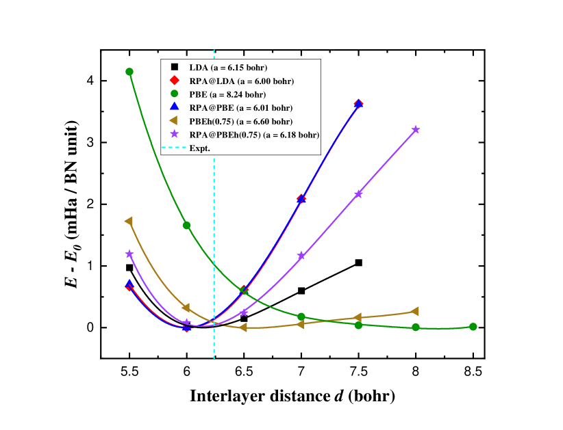
Figure 6: Energy as a function of the spacing between the layers for hexagonal BN with different gKS approximations and different starting points for RPA.

In order to test if the weak van der Waals interactions would correctly be described by sc$GW$, we analyzed a layered material, namely the hexagonal BN (h-BN). RPA@LDA or RPA@PBE were proven to be able to describe properly the spacing between the layers [67, 13].

The task of evaluating the $\gamma^{GW}$ for h-BN is beyond our current computational capabilities. Indeed, for the weak van der Waals interactions, the energy scales are so low that extremely converged calculations are required. Fortunately, based on the previous discussion, we assume that the sc$GW$ total energy is also well approximated by RPA@PBEh(0.75).

In Fig. 6, we report the energy versus spacing between the layers. LDA is known to give the correct spacing thanks to a lucky compensation of errors [67], whereas PBE that improves the exchange over LDA does not benefit from this and yields a much too large spacing. Our RPA@LDA reproduces within 0.25 bohr the earlier estimates from Refs. 67, 13. This agreement is quite good considering the computational power difference and considering the fact that we use newly developed pseudopotentials.

Next, let us comment that the RPA@PBEh(0.75) result (see Fig. 6) shows our best approximate to the sc$GW$. The obtained lattice spacing is very good agreement with respect to the experiment (6.18 bohr against 6.25 bohr).

This example shows that tuning the starting point in RPA does not destroy the quantitative agreement with respect to the experiment. This interesting conclusion calls for further studies in the future.

VI Conclusion

The linearized $GW$ density matrix $\gamma^{GW}$ has been introduced in realistic solid-state systems. We have carefully tested the norm-conserving pseudopotential approximation and have concluded that QMC pseudopotentials, such as ccECP [59], are compulsory in this context for accurately determining RPA and $\gamma^{GW}$ lattice constants. On a benchmark of 7 covalent crystals (Si, C, SiC, zb-BN, AlP, AlAs, and Ge), we have proven numerically that $\gamma^{GW}$ actually fulfils the exact constraints: its natural occupation numbers range from 0 to 2 (when spin is summed) and they sum up to the correct number of electrons. In addition, the correlated nature of $\gamma^{GW}$ allows the electron occupancy to reorganize across the Brillouin zone, in strong contrast with all the mean-field approaches, where the electron count remains constant in the Brillouin zone for crystals with a band gap.

The one-shot total energy expression $E_{\mathrm{total}}^{\gamma^{GW}}$ has been found to be superior to the usual RPA total energy expression in terms of sensitivity to the gKS starting point.

We provide strong evidence to support the assumption that $\gamma^{GW}$-based total energy is a reliable substitute for sc$GW$, which remains unachievable at present. As a cheaper alternative, RPA can also be used, but we advocate applying it on top of gKS functionals with a large content of the exact exchange, at least 75 %, such as PBEh(0.75) or HF to best approximate sc$GW$. Our last statement disagrees with the current wisdom that recommends RPA@PBE based on comparison to experiment.

Our implementation is available in the public version the open source code ABINIT [68].

Appendix A The unit cell density matrix in the natural orbital representation.

The density matrix $\gamma(\mathbf{r},\mathbf{r}^{\prime})$ is diagonal in $\mathbf{k}$

Imposing the Born-van Karman periodic conditions, we can write the double-Fourier expansion of $\gamma(\mathbf{r},\mathbf{r}^{\prime})$ in reciprocal space as

$$\gamma({\bf r},{\bf r}^{\prime})=\frac{1}{N_{k}\Omega}\sum_{\mathbf{k}\mathbf{k}^{\prime}\mathbf{G}\mathbf{G}^{\prime}}e^{\mathrm{i}(\mathbf{k}+\mathbf{G})\cdot\mathbf{r}}\gamma_{\mathbf{k}\mathbf{k}^{\prime}}(\mathbf{G},\mathbf{G}^{\prime})e^{-\mathrm{i}(\mathbf{k}^{\prime}+\mathbf{G}^{\prime})\cdot\mathbf{r}^{\prime}},$$ (23)

where $N_{k}$ is the number of k-points and $\Omega$ is the volume of the unit cell and $\mathbf{G}$ and $\mathbf{G}^{\prime}$ are reciprocal lattice vectors.

By virtue of the translation invariance in the unit cell, the shift of the two space indices with ${\bf R}=n_{1}{\bf a}_{1}+n_{2}{\bf a}_{2}+n_{3}{\bf a}_{3}$ (with $n_{1},n_{2},n_{3}\in\mathbb{Z}$ and ${\bf a}_{1},{\bf a}_{2},{\bf a}_{3}$ being the primitive lattice vectors) does not change the density matrix [69]:

$$\gamma({\bf r},{\bf r}^{\prime})=\gamma({\bf r}+{\bf R},{\bf r}^{\prime}+{\bf R}).$$ (24)

When inserting the double Fourier transform, this implies

$$e^{\mathrm{i}(\mathbf{k}-\mathbf{k}^{\prime})\cdot\mathbf{R}}=1.$$ (25)

This condition is fulfilled if and only if $(\mathbf{k}-\mathbf{k}^{\prime})$ belongs to the reciprocal lattice. And as $\mathbf{k}$ and $\mathbf{k}^{\prime}$ both belong to the first Brillouin zone, the only possible reciprocal lattice vector the difference can match is $\mathbf{0}$.

As a consequence, one can insert the Kronecker sign $\delta_{\mathbf{k}\mathbf{k}^{\prime}}$ in Eq. (23):

$$\gamma({\bf r},{\bf r}^{\prime})=\frac{1}{N_{k}\Omega}\sum_{\mathbf{k}\mathbf{G}\mathbf{G}^{\prime}}e^{\mathrm{i}(\mathbf{k}+\mathbf{G})\cdot\mathbf{r}}\gamma_{\mathbf{k}}(\mathbf{G},\mathbf{G}^{\prime})e^{-\mathrm{i}(\mathbf{k}+\mathbf{G}^{\prime})\cdot\mathbf{r}^{\prime}}$$ (26)

and obtain the desired expression that shows that $\gamma$ is block-diagonal with respect to $\mathbf{k}$.

Natural orbitals and occupations

Now for each discrete value of $\mathbf{k}$, one can diagonalize $\gamma_{\mathbf{k}}$:

$$\sum_{\mathbf{G}^{\prime}}\gamma_{\mathbf{k}}(\mathbf{G},\mathbf{G}^{\prime})\tilde{u}_{\mathbf{k}\lambda}(\mathbf{G}^{\prime})=n_{\mathbf{k}\lambda}\tilde{u}_{\mathbf{k}\lambda}(\mathbf{G}),$$ (27)

where $\tilde{u}_{\mathbf{k}\lambda}(\mathbf{G})$ are the eigenvectors and $n_{\mathbf{k}\lambda}$ the eigenvalues, indexed with $\lambda$.

By construction:

$$\gamma(\mathbf{r},\mathbf{r}^{\prime})=\gamma(\mathbf{r}^{\prime},\mathbf{r})^{*}$$ (28)

implies

$$\gamma_{\mathbf{k}}(\mathbf{G},\mathbf{G}^{\prime})=\gamma_{\mathbf{k}}(\mathbf{G}^{\prime},\mathbf{G})^{*}$$ (29)

$\gamma_{\mathbf{k}}(\mathbf{G},\mathbf{G}^{\prime})$ is an Hermitian matrix and thus the $n_{\mathbf{k}\lambda}$ are real-valued and the $\tilde{u}_{\mathbf{k}\lambda}$ form a unitary matrix

Using this decomposition,

$$\gamma_{\mathbf{k}}(\mathbf{G},\mathbf{G}^{\prime})=\sum_{\lambda}n_{\mathbf{k}\lambda}\tilde{u}_{\mathbf{k}\lambda}(\mathbf{G})\tilde{u}_{\mathbf{k}\lambda}^{*}(\mathbf{G}^{\prime}),$$ (30)

Inserting this in Eq. (26), we obtain

$$\gamma(\mathbf{r},\mathbf{r}^{\prime})=\frac{1}{N_{k}\Omega}\sum_{\mathbf{k}\lambda}\sum_{\mathbf{G}}e^{\mathrm{i}(\mathbf{k}+\mathbf{G})\cdot\mathbf{r}}\tilde{u}_{\mathbf{k}\lambda}(\mathbf{G})\\ \times n_{\mathbf{k}\lambda}\sum_{\mathbf{G}^{\prime}}\tilde{u}_{\mathbf{k}\lambda}^{*}(\mathbf{G}^{\prime})e^{-\mathrm{i}(\mathbf{k}+\mathbf{G}^{\prime})\cdot\mathbf{r}^{\prime}}$$ (31)

Let us introduce the natural orbital in real-space $\phi_{\mathbf{k}\lambda}(\mathbf{r})$ that have a Bloch’s wave form [70]:

$$\phi_{\mathbf{k}\lambda}(\mathbf{r}) =\frac{1}{\sqrt{N_{k}\Omega}}\sum_{\mathbf{G}}e^{\mathrm{i}(\mathbf{k}+\mathbf{G})\cdot\mathbf{r}}\tilde{u}_{\mathbf{k}\lambda}(\mathbf{G})$$ (32)

$$=\frac{1}{\sqrt{N_{k}\Omega}}e^{\mathrm{i}\mathbf{k}\cdot\mathbf{r}}\tilde{u}_{\mathbf{k}\lambda}(\mathbf{r})$$ (33)

The final expression in real space reads

$$\gamma(\mathbf{r},\mathbf{r}^{\prime})=\sum_{\mathbf{k}\lambda}n_{\mathbf{k}\lambda}\phi_{\mathbf{k}\lambda}(\mathbf{r})\phi_{\mathbf{k}\lambda}^{*}(\mathbf{r}^{\prime}).$$ (34)

that looks extremely similar to the mean-field (gKS) expression

$$\gamma^{\mathrm{gKS}}(\mathbf{r},\mathbf{r}^{\prime})=\sum_{\mathbf{k}i}f_{\mathbf{k}i}\varphi_{\mathbf{k}i}(\mathbf{r})\varphi_{\mathbf{k}i}^{*}(\mathbf{r}^{\prime}),$$ (35)

where $f_{\mathbf{k}i}$ are the Fermi-Dirac occupations and $\varphi_{\mathbf{k}i}(\mathbf{r})$ the mean-field wavefunctions.

However, there are subtle differences that are much more meaningful:

• In gKS DFT, $\varphi_{\mathbf{k}i}(\mathbf{r})$ sum up to the exact electronic density, whereas the natural orbital sum up to the exact density and density matrix.

• For the ground-state, the spin-summed $f_{\mathbf{k}i}$ are constrained to be 0 or 2, whereas the spin-summed $n_{\mathbf{k}\lambda}$ continuously span the range from 0 to 2 (not proven here).

• Since $\int d\mathbf{r}\gamma(\mathbf{r},\mathbf{r})$ is normalized to the number of electrons $N_{e}$, both $f_{\mathbf{k}i}$ and $n_{\mathbf{k}\lambda}$ sum up to $N_{e}$. However, for insulators, while $\sum_{i}f_{\mathbf{k}i}=N_{e}$, for each $\mathbf{k}$ individually, no equivalent exists for the natural occupations $n_{\mathbf{k}\lambda}$. as we show in the appendix B.

Appendix B Non-integer $N(\mathbf{k})$ values for individual $\mathbf{k}$

The non-integer values reported for the electron count, $N({\bf k})$, are a consequence of the electron correlation effects. In this appendix, we gain some insights into this result.

B.1 The many-electron wavefunction in crystals

The basis of Bloch waves is complete; therefore, the real-space $N$-electron wavefunction can be written as a linear combination of Slater determinants $\left[(N!)^{-1/2}|\varphi_{\mathbf{k}_{\mu}i}(\mathbf{r}_{1})\ldots\varphi_{\mathbf{k}_{\nu}j}(\mathbf{r}_{N})|\right]$ built using Bloch waves,

$$\varphi_{\mathbf{k}i}(\mathbf{r})=\frac{1}{\sqrt{N_{k}\Omega}}\sum_{G}e^{\mathrm{i}\mathbf{k}\cdot\mathbf{r}}u_{\mathbf{k}i}(\mathbf{r}),$$ (36)

which are usually the ones obtained from a mean-field method (like the ones obtained from a gKS DFT calculation). However, other basis sets can be used to build the Slater determinants, such as the Bloch waves corresponding to the natural orbitals. In this representation, the real-space (spin-less) $N$-electron wavefunction can be written as a configuration interaction (CI) expansion

$$\Psi(\mathbf{r}_{1},\mathbf{r}_{2},...,\mathbf{r}_{N})=\frac{1}{\sqrt{N!}(\sqrt{N_{k}\Omega})^{N}}\sum_{\mathbf{k}_{\mu}\ldots\mathbf{k}_{\nu}}\sum_{i\in\Omega_{\mathbf{k}_{\mu}}}\ldots\sum_{j\in\Omega_{\mathbf{k}_{\nu}}}C_{\mathbf{k}_{\mu}i\ldots\mathbf{k}_{\nu}j}e^{\mathrm{i}\left(\mathbf{k}_{\mu}\cdot\mathbf{r}_{1}+\ldots+\mathbf{k}_{\nu}\cdot\mathbf{r}_{N}\right)}u_{\mathbf{k}_{\mu}i}(\mathbf{r}_{1})\dots u_{\mathbf{k}_{\nu}j}(\mathbf{r}_{N}),$$ (37)

where the sum $\sum_{\mathbf{k}_{\mu}\ldots\mathbf{k}_{\nu}}$ runs over all k-points in the first Brillouin zone, and the $C_{\mathbf{k}_{\mu}i\ldots\mathbf{k}_{\nu}j}$ are the expansion coefficients (that are adequately adjusted to ensure that $\Psi$ preserves the correct symmetries). Let us highlight that in Eq. (37), the Hartree product of Bloch’s waves contains waves that belong to different k-points (i.e. $\Psi$ is the many-body wavefunction of the supercell).

The Born-van Karman periodic conditions imposed to the many-electron wavefunction [71] state that $\Psi(\mathbf{r}_{1},\mathbf{r}_{2},...,\mathbf{r}_{N})=\Psi(\mathbf{r}_{1}+{\bf T},\mathbf{r}_{2}+{\bf T},...,\mathbf{r}_{N}+{\bf T})$ for ${\bf T}=n_{1}N_{1}{\bf a}_{1}+n_{2}N_{2}{\bf a}_{2}+n_{3}N_{3}{\bf a}_{3}$ (with $N_{k}=N_{1}N_{2}N_{3}$). As a consequence, $e^{\mathrm{i}\left(\mathbf{k}_{\mu}+\ldots+\mathbf{k}_{\nu}\right)\cdot{\bf T}}=e^{\mathrm{i}{\bf K}\cdot{\bf T}}=1$ and

$${\bf K} =\mathbf{k}_{\mu}+\ldots+\mathbf{k}_{\nu}$$ (38)

$$=\frac{\chi_{1}}{N_{1}}{\bf b}_{1}+\frac{\chi_{2}}{N_{2}}{\bf b}_{2}+\frac{\chi_{3}}{N_{3}}{\bf b}_{3},$$ (39)

where $\chi_{n}\in\mathbb{Z}$. The many-electron wavefunctions are eigenfunctions of the many-body translation operator $\widehat{T}_{\bf R}$, i.e.

$$\widehat{T}_{\bf R}\Psi_{\bf K}(\mathbf{r}_{1},\mathbf{r}_{2},...,\mathbf{r}_{N}) =\Psi_{\bf K}(\mathbf{r}_{1}+{\bf R},\mathbf{r}_{2}+{\bf R},...,\mathbf{r}_{N}+{\bf R})$$ (40)

$$=e^{\mathrm{i}{\bf K}\cdot{\bf R}}\Psi_{\bf K}(\mathbf{r}_{1},\mathbf{r}_{2},...,\mathbf{r}_{N}),$$ (41)

with $e^{\mathrm{i}{\bf K}\cdot{\bf R}}$ eigenvalues. Since the many-body Hamiltonian $\widehat{H}$ (within the Born-Oppenheimer approximation) commutes with the $\widehat{T}_{\bf R}$ operator [71], the solutions to the many-body Hamiltonian can be taken associated with a given ${\bf K}$ value (i.e. $\widehat{H}\Psi_{\bf K}=E\Psi_{\bf K}$). Actually, the many-electron wavefunctions associated with ${\bf K}+\mathbf{G}$ (with $\mathbf{G}=\chi_{1}{\bf b}_{1}+\chi_{2}{\bf b}_{2}+\chi_{3}{\bf b}_{3}$ being a reciprocal lattice vector) also lead to the same eigenvalue $e^{\mathrm{i}{\bf K}\cdot{\bf R}}$ upon application of the $\widehat{T}_{\bf R}$ operator and may contribute to the CI expansion.

B.2 The density matrix and the second-order reduced density matrix in crystals

Let us define the density matrix elements (from the many-body wavefunction $\Psi$) as

$$\gamma_{\mathbf{k}ij}=\langle\Psi|\widehat{b}^{\dagger}_{\mathbf{k}i}\widehat{b}_{\mathbf{k}j}|\Psi\rangle$$ (42)

and the second-order reduced density matrix (2-RDM) matrix elements as

$$\Gamma_{\mathbf{k}_{\mu}i,\mathbf{k}_{\nu}l}^{\mathbf{k}_{\tau}j,\mathbf{k}_{\vartheta}m}=\frac{1}{2}\langle\Psi|\widehat{b}^{\dagger}_{\mathbf{k}_{\mu}i}\widehat{b}^{\dagger}_{\mathbf{k}_{\nu}l}\widehat{b}_{\mathbf{k}_{\vartheta}m}\widehat{b}_{\mathbf{k}_{\tau}j}|\Psi\rangle$$ (43)

whose $\mathbf{k}_{n}$ values fulfill the condition

$$\mathbf{k}_{\mu}+\mathbf{k}_{\nu}-\mathbf{k}_{\tau}-\mathbf{k}_{\vartheta}+{\bf G}=0,$$ (44)

which ensures the correct translational symmetry of the 2-RDM, i.e.

$$\Gamma({\bf r}_{1},{\bf r}_{2},{\bf r}_{1}^{\prime},{\bf r}_{2}^{\prime})=\Gamma({\bf r}_{1}+{\bf R},{\bf r}_{2}+{\bf R},{\bf r}_{1}^{\prime}+{\bf R},{\bf r}_{2}^{\prime}+{\bf R}),$$ (45)

where $\Gamma({\bf r}_{1},{\bf r}_{2},{\bf r}_{1}^{\prime},{\bf r}_{2}^{\prime})$ is the 2-RDM in space representation (see for example Refs. [72, 73] for more details). The 2-RDM contains more information about the system than the density matrix. Indeed, the matrix elements of the density matrix can be obtained from the partial trace of the 2-RDM:

$$\gamma_{\mathbf{k}ij}=\frac{2}{N-1}\sum_{\mathbf{k}^{\prime}}\sum_{l\in\Omega_{\mathbf{k}^{\prime}}}\Gamma_{\mathbf{k}i,\mathbf{k}^{\prime}l}^{{\mathbf{k}j,\mathbf{k}^{\prime}l}},$$ (46)

where $\Omega_{\mathbf{k}^{\prime}_{\nu}}$ is the subspace formed by all the one-electron wavefunctions sharing the same ${\mathbf{k}^{\prime}_{\nu}}$ value. For completeness, let us mention that the matrix formed using the $\gamma_{\mathbf{k}ij}$ elements is Hermitian and upon diagonalization produces the occupation numbers $n_{\mathbf{k}\lambda}$ discussed in the appendix A.

B.3 The APSG ansatz for crystals

Here we prove in the specific case of an anti-symmetrized product of strongly-orthogonal geminals (APSG) ansatz [74] for the many-electron wavefunction that electron count transfer can occur across k-points due to electronic correlation effects. If it is true for this subclass of wavefunctions, then the statement also holds for the exact wavefunction.

The APSG ansatz for the many-electron wavefunction with spin, where an even number of electrons present in the system is assumed (as we employed throughout this work) reads

$$\Psi^{\textrm{APSG}}_{\bf K}(\mathbf{x}_{1},\mathbf{x}_{2},...,\mathbf{x}_{N})=\widehat{A}\prod^{N/2}_{P=1}\psi_{P}(\mathbf{x}_{2P-1},\mathbf{x}_{2P}),$$ (47)

where $\mathbf{x}=(\mathbf{r},\sigma)$ is spatial and spin coordinate with $\sigma=\alpha,\beta$ referring to the spin index, $\widehat{A}$ stands for the antisymmetrizer responsible for inter-geminal permutations of electron coordinates and the geminal wavefunctions $\psi_{P}(\mathbf{x}_{2P-1},\mathbf{x}_{2P})$ are wavefunctions containing one $\alpha$ and one $\beta$ electron. Because of this, the geminal wavefunction is a two-electron wavefunction; the sum of the occupation numbers for each spin channel must be

$$\sum_{\left[\mathbf{k},i\in\Omega_{\mathbf{k}}\right]\in P}n_{\mathbf{k}i}=1$$ (48)

with $\left[\mathbf{k},i\in\Omega_{\mathbf{k}}\right]\in P$ indicating that the $i$-th Bloch’s wave belonging to the $\mathbf{k}$-th k-point (i.e. the Bloch’s wave natural orbital $\phi_{\mathbf{k}i}$) is one of the Bloch’s waves used in the construction of the $P$-th geminal. The $P$-th geminal wavefunction written in terms of the natural orbital Bloch’s waves reads as

$$\psi_{P}(\mathbf{x}_{2P-1},\mathbf{x}_{2P})=2^{-1/2}\sum_{\left[\mathbf{k},i\in\Omega_{\mathbf{k}}\right]\in P}c_{\mathbf{k}i}\left[\phi_{\mathbf{k}i}({\bf r}_{2P-1})\alpha_{2P-1}\phi^{*}_{\mathbf{k}i}({\bf r}_{2P})\beta_{2P}-\phi_{\mathbf{k}i}({\bf r}_{2P})\alpha_{2P}\phi^{*}_{\mathbf{k}i}({\bf r}_{2P-1})\beta_{2P-1}\right],$$ (49)

where the time-reversal symmetry is being employed to relate the degenerated Bloch’s waves containing electrons with opposite spin [75, 76] forming a Kramers’ pairs (i.e. $\phi_{\mathbf{k}i}$ and $\phi^{*}_{\mathbf{k}i}$ form a Kramers’ pair). Let us remark that the presence of complex-conjugated Bloch’s waves (natural orbitals) is related to states filled by $\beta$ spin electrons; this choice is completely arbitrary. Also, the time-reversal symmetry imposed on the many-electron wavefunction leads to $\Psi_{{\bf K}={\bf 0}}$ for spin-compensated systems.

Since the $\{\psi_{P}\}$ geminal wavefunctions are built with the strong orthonormality requirement, i.e. the condition that $\forall_{P\neq Q}\;\int d\mathbf{x}_{2}\psi_{P}(\mathbf{x}_{1},\mathbf{x}_{2})\psi_{Q}(\mathbf{x}_{1}^{\prime},\mathbf{x}_{2})=\delta_{PQ}$, then the Bloch’s waves natural orbitals are present in only one geminal wavefunction. When all the $\psi_{P}$ are built containing only one Kramers’ pair as

$$\psi_{P}(\mathbf{x}_{2P-1},\mathbf{x}_{2P}) =2^{-1/2}\left[\phi_{\mathbf{k}i}({\bf r}_{2P-1})\alpha_{2P-1}\phi^{*}_{\mathbf{k}i}({\bf r}_{2P})\beta_{2P}-\phi_{\mathbf{k}i}({\bf r}_{2P})\alpha_{2P}\phi^{*}_{\mathbf{k}i}({\bf r}_{2P-1})\beta_{2P-1}\right],$$ (50)

the many-body wavefunction ($\Psi_{\bf K}$) defined in Eq. (47) corresponds to a single Slater determinant; thus, the Hartree-Fock approximation is recovered, where the natural orbital basis and the so-called canonical orbitals (the mean-field ones) coincide.

The structure of the APSG wavefunction allows us to express the total energy in terms of the natural orbitals, the occupation numbers, and some undetermined phases. Then, the total APSG energy takes the following form

$$E^{\textrm{APSG}}\left[\{f_{\mathbf{k}_{\mu}i}\},\{n_{\mathbf{k}_{\mu}i}\},\{\phi_{\mathbf{k}_{\mu}i}\}\right] =2\sum_{\mathbf{k}_{\mu}}\sum_{i\in\Omega_{\mathbf{k}_{\mu}}}n_{\mathbf{k}_{\mu}i}\langle\mathbf{k}_{\mu}i|\widehat{h}|\mathbf{k}_{\mu}i\rangle$$

$$+\sum^{N/2}_{P}\sum\limits_{\begin{subarray}{c}\left[\mathbf{k}_{\mu},i\in\Omega_{\mathbf{k}_{\mu}}\right]\\ \left[\mathbf{k}_{\nu},j\in\Omega_{\mathbf{k}_{\nu}}\right]\end{subarray}\in P}\zeta_{\mathbf{k}_{\mu}i}\zeta_{\mathbf{k}_{\nu}j}\sqrt{n_{\mathbf{k}_{\mu}i}n_{\mathbf{k}_{\nu}j}}\langle{\mathbf{k}_{\mu}i}{\mathbf{k}_{\nu}j}|{\mathbf{k}_{\nu}j}{\mathbf{k}_{\mu}i}\rangle$$ (51)

$$+\sum^{N/2}_{P\neq Q}\sum\limits_{\begin{subarray}{c}\left[\mathbf{k}_{\mu},i\in\Omega_{\mathbf{k}_{\mu}}\right]\in P\\ \left[\mathbf{k}_{\nu},j\in\Omega_{\mathbf{k}_{\nu}}\right]\in Q\end{subarray}}n_{\mathbf{k}_{\mu}i}n_{\mathbf{k}_{\nu}j}(2\langle{\mathbf{k}_{\mu}i\mathbf{k}_{\nu}j}|{\mathbf{k}_{\mu}i\mathbf{k}_{\nu}j}\rangle-\langle{\mathbf{k}_{\mu}i\mathbf{k}_{\nu}j}|{\mathbf{k}_{\nu}j}{\mathbf{k}_{\mu}i}\rangle),$$

where we have employed the known condition for APSG wavefunctions that allows us to express the CI coefficients in terms of occupation numbers ($c^{2}_{\mathbf{k}i}=n_{\mathbf{k}i}$ or $c_{\mathbf{k}i}=\zeta_{\mathbf{k}i}\sqrt{n_{\mathbf{k}i}}$), the phases $\zeta_{\mathbf{k}_{\mu}i}^{2}=1$, $\widehat{h}$ refers to all one-body operators of the electronic Hamiltonian (i.e. the kinetic energy and the interaction with the external potential), $\langle{\mathbf{k}_{\mu}i\mathbf{k}_{\nu}j}|{\mathbf{k}_{\tau}k\mathbf{k}_{\vartheta}l}\rangle$ are the usual two-electron integrals. Notice that the energy minimization procedure implies optimization of the occupation numbers, natural orbitals, and phases. Since this wavefunction can be entirely written in terms of the natural orbitals and occupation numbers, it has been widely used in the context of reduced density matrix functional theory to propose energy functionals [77, 78, 79, 80, 81, 82, 83, 84, 85].

The energy contribution in the second line of Eq. (B.3) is coming from the geminal wavefunctions and describes intra-geminal interactions (i.e. the ones among the two electrons belonging to the geminal wavefunction). On the other hand, energy contribution in the third line of Eq. (B.3) describes inter-geminal interactions, which are taken at the mean-field level (i.e. as Hartree–Fock interactions). Also, let us highlight that imposing the correct translation symmetry to $\Psi^{\textrm{APSG}}_{\bf K}$ automatically enforces the correct symmetry in the 2-RDM elements. Making the 2-RDM elements fulfill the condition presented in Eq. (44).

Since the natural orbitals belonging to different $\Omega_{\mathbf{k}}$ subspaces (e.g. $\mathbf{k}$ and $\mathbf{k}^{\prime}$) can be employed in the construction of the geminal wavefunctions (see Eq. (49)) the constraint given by Eq. (44) takes the following form for the geminals wavefunction

$$\mathbf{k}^{\prime}-\mathbf{k}^{\prime}-\mathbf{k}+\mathbf{k}={\bf 0}=\mathbf{G},$$ (52)

which ensures the correct translation symmetry in $\Psi^{\textrm{APSG}}_{\bf K}$, the 2-RDM matrix elements, and the density matrix. Notice that the complex conjugation associated with the time-reversal symmetry of the Kramers’ pairs was employed.

The occupation numbers of the natural orbitals that belong to the geminal are optimized under the constraint given in Eq. (48) during the energy minimization procedure (recalling that the CI coefficients can be written as $c_{\mathbf{k}i}=\zeta_{\mathbf{k}i}\sqrt{n_{\mathbf{k}i}}$ for the $\Psi^{\textrm{APSG}}_{\bf K}$ ansatz). Hence, the coupling of natural orbitals belonging to different k-points is allowed; thus, a reorganization of electrons among k-points can take place during the energy minimization procedure. Moreover, it is known [86] that the occupation numbers are not likely to become zero; then, the reorganization of electrons among k-points is not forbidden.

In summary, the $\Psi^{\textrm{APSG}}_{\bf K}$ ansatz is a valid approximation to the many-electron wavefunction that permits us to illustrate the reasons leading to the reorganization of electrons among k-points. Obviously, a more general valid CI expansion ansatz (or the exact full-CI expansion) could also lead to a reorganization of the electrons among k-points since the $\Psi^{\textrm{APSG}}_{\bf K}$ ansatz is a particular case of the exact $\Psi_{\bf K}$, where the electron pairs do not interact. Then, let us conclude that the reorganization of electrons among k-points that lead to non-integer $N_{e}$ values for each $\mathbf{k}$ value is purely a consequence of the electronic correlation effects. In this work, the electronic correlation effects are captured with the $\gamma^{GW}$ approximation, which produces the reorganization of electrons among k-points. And, this leads to the non-integer $N_{e}$ values obtained for each k-point that were used to compute the $\Delta N({\mathbf{k}})$ values presented in Fig. 3.

In the next section, we present an example based on the Si crystal where the reorganization of electrons among k-points is allowed using a $\Psi^{\textrm{APSG}}_{\bf K}$ ansatz.

B.4 Example of an allowed electronic density reorganization among the k-points in the Si crystal

For a working example, let us take the Si crystal computed excluding all the core states (i.e. using a pseudo-potential and retaining only 8 electrons per unit cell). At the Hartree–Fock (or gKS DFT) level, eight states forming four Kramers’ pairs are occupied for each k-point value. From the band structure, it is easy to recognize that the highest (in terms of energy) occupied state with an $\alpha$ electron localized at the $\Gamma$ point ($\mathbf{k}=(0,0,0)=\mathbf{k}_{\Gamma}$). On the other hand, the lowest (in terms of energy) unoccupied state for the electrons with $\alpha$ spin belongs to the $X$ point ($\mathbf{k}=(0.5,0.5,0)=\mathbf{k}_{X}$). Let us label these states as $\varphi_{\mathbf{k}_{\Gamma}4}$ and $\varphi_{\mathbf{k}_{X}5}$, respectively. The energy difference between the $\varphi_{\mathbf{k}4}$ and $\varphi_{\mathbf{k}5}$ states is small (the experimental value is approximately 1 eV), which leads to the small indirect band gap obtained for this system.

Following, let us organize in ascending order in terms of energy all the mean-field Bloch’s waves for the whole system (i.e. of the supercell). And, as it is usually done in the search for the optimal $\Psi^{\textrm{APSG}}_{{\bf K}={\bf 0}}$, let us write the initial guess for the APSG ansatz in terms of the mean-field Bloch’s waves. But, let us search for a particular $\Psi^{\textrm{APSG}}_{\bf K}$ ansatz where all the geminal wavefunctions contain only one Kramers’ pair (i.e. are treated at the Hartree–Fock level) except for the last geminal (the $P=N/2$ in (49)) that is built coupling the Bloch’s waves $\varphi_{\mathbf{k}_{\Gamma}4}$ and $\varphi_{\mathbf{k}_{X}5}$, i.e.

$$\psi_{N/2}(\mathbf{x}_{N-1},\mathbf{x}_{N}) =2^{-1/2}\left[c_{\mathbf{k}_{\Gamma}4}(\varphi_{\mathbf{k}_{\Gamma}4}(\mathbf{r}_{N-1})\alpha_{N-1}\varphi^{*}_{\mathbf{k}_{\Gamma}4}(\mathbf{r}_{N})\beta_{N}+\varphi_{\mathbf{k}_{\Gamma}4}(\mathbf{r}_{N})\alpha_{N}\varphi^{*}_{\mathbf{k}_{\Gamma}4}(\mathbf{r}_{N-1})\beta_{N-1})\right.$$ (53)

$$+\left.c_{\mathbf{k}_{X}5}(\varphi_{\mathbf{k}_{X}5}(\mathbf{r}_{N-1})\alpha_{N-1}\varphi^{*}_{\mathbf{k}_{X}5}(\mathbf{r}_{N})\beta_{N}+\varphi_{\mathbf{k}_{X}5}(\mathbf{r}_{N})\alpha_{N}\varphi^{*}_{\mathbf{k}_{X}5}(\mathbf{r}_{N-1})\beta_{N-1})\right],$$

with $c_{\mathbf{k}_{\Gamma}4}=\zeta_{\mathbf{k}_{\Gamma}4}\sqrt{n_{\mathbf{k}_{\Gamma}4}}$ and $c_{\mathbf{k}_{X}5}=\zeta_{\mathbf{k}_{X}5}\sqrt{n_{\mathbf{k}_{X}5}}$ being variational parameters subject to the condition $n_{\mathbf{k}_{\Gamma}4}+n_{\mathbf{k}_{X}5}=1$ (to fulfill the requirement presented in Eq. (48)). This type of geminal approach, where only two states (four considering spin) are present in the geminal wavefunction is known as a perfect-pairing approach. Next, let us assume that the mean-field Bloch’s waves $\varphi_{\mathbf{k}_{\Gamma}4}$ and $\varphi_{\mathbf{k}_{X}5}$ coincide with the optimal natural orbitals in order to skip the orbital optimization procedure.

Next, let us focus on the energy contribution arising from the ${N/2}$ geminal to the second term in the r.h.s. of the APSG energy (see Eq. (B.3))

$$n_{\mathbf{k}_{\Gamma}4}\langle{\mathbf{k}_{\Gamma}4}{\mathbf{k}_{\Gamma}4}|{\mathbf{k}_{\Gamma}4}{\mathbf{k}_{\Gamma}4}\rangle+n_{\mathbf{k}_{X}5}\langle{\mathbf{k}_{X}5}{\mathbf{k}_{X}5}|{\mathbf{k}_{X}5}{\mathbf{k}_{X}5}\rangle+2\zeta_{\mathbf{k}_{\Gamma}4}\zeta_{\mathbf{k}_{X}5}\sqrt{n_{\mathbf{k}_{\Gamma}4}n_{\mathbf{k}_{X}5}}\langle{\mathbf{k}_{\Gamma}4}{\mathbf{k}_{X}5}|{\mathbf{k}_{X}5}{\mathbf{k}_{\Gamma}4}\rangle.$$ (54)

Setting the usual approximation for (fixing) the phases (i.e. $\zeta_{\mathbf{k}_{\Gamma}4}\zeta_{\mathbf{k}_{X}5}=-1$ [77, 78, 81, 80]) for the interaction among the states above and below the Fermi level and letting all two-electron integrals to be equal (which can occur in the extreme case when degenerated states are involved). The occupation numbers that would minimize the energy contribution are $n_{\mathbf{k}_{\Gamma}4}=n_{\mathbf{k}_{X}5}=1/2$. Illustrating that a reorganization of electrons occurs among the $\Gamma$ and $X$ k-points. In the Si crystal, the mean-field Bloch’s waves are not completely degenerate in terms of energy and do not correspond to the optimal natural orbitals; then, the actual optimal occupation numbers differ from $1/2$. But, they also differ from the initial values at the mean-field level, where $n_{\mathbf{k}_{\Gamma}4}=1$ and $n_{\mathbf{k}_{X}5}=0$. Moreover, beyond the perfect pairing approach, the coupling of states to form a geminal wavefunction can include states belonging to other k-points. Since the geminal wavefunctions are built with states for the $\alpha$ and the $\beta$ electron; the state for the $\alpha$ electrons is associated with a $\mathbf{k}^{\prime\prime}$ k-point while the state for the $\beta$ is related to a $-\mathbf{k}^{\prime\prime}$ k-point. The Hartree product in Eq. (49) conserves the ${\bf K}=\mathbf{k}^{\prime\prime}-\mathbf{k}^{\prime\prime}={\bf 0}$ value, which could lead to further reorganization of electrons among different k-points beyond the perfect pairing approach. Thus, for example, the coupling of states belonging to $\Gamma$, $X$, and $\Delta$, etc. is allowed in the Si crystal. Actually, the coupling of all k-point values in the first Brillouin zone is valid to build geminal wavefunctions.

Finally, let us remark that this example is based on a valid approximation to the many-electron wavefunction (i.e. a $\Psi^{\textrm{APSG}}_{\bf K}$ ansatz), where we illustrate that the reorganization of electrons among k-points is purely a consequence of the electronic correlation effects.

References

- Ku and Eguiluz [2002] W. Ku and A. G. Eguiluz, Band-gap problem in semiconductors revisited: Effects of core states and many-body self-consistency, Phys. Rev. Lett. 89, 126401 (2002).
- Cao et al. [2017] H. Cao, Z. Yu, P. Lu, and L.-W. Wang, Fully converged plane-wave-based self-consistent calculations of periodic solids, Phys. Rev. B 95, 035139 (2017).
- Grumet et al. [2018] M. Grumet, P. Liu, M. Kaltak, J. Klimeš, and G. Kresse, Beyond the quasiparticle approximation: Fully self-consistent calculations, Phys. Rev. B 98, 155143 (2018).
- Holm [1999] B. Holm, Total energies from calculations, Phys. Rev. Lett. 83, 788 (1999).
- García-González and Godby [2001] P. García-González and R. W. Godby, Self-consistent calculation of total energies of the electron gas using many-body perturbation theory, Phys. Rev. B 63, 075112 (2001).
- Kutepov et al. [2009] A. Kutepov, S. Y. Savrasov, and G. Kotliar, Ground-state properties of simple elements from gw calculations, Phys. Rev. B 80, 041103 (2009).
- Dobson and Wang [1999] J. F. Dobson and J. Wang, Successful test of a seamless van der waals density functional, Phys. Rev. Lett. 82, 2123 (1999).
- García-González and Godby [2002] P. García-González and R. W. Godby, Many-body calculations of ground-state properties: Quasi-2d electron systems and van der waals forces, Phys. Rev. Lett. 88, 056406 (2002).
- Harl and Kresse [2008] J. Harl and G. Kresse, Cohesive energy curves for noble gas solids calculated by adiabatic connection fluctuation-dissipation theory, Phys. Rev. B 77, 045136 (2008).
- Lu et al. [2009] D. Lu, Y. Li, D. Rocca, and G. Galli, Ab initio calculation of van der waals bonded molecular crystals, Phys. Rev. Lett. 102, 206411 (2009).
- Schimka et al. [2010] L. Schimka, J. Harl, A. Stroppa, A. Grueneis, M. Marsman, F. Mittendorfer, and G. Kresse, Accurate surface and adsorption energies from many-body perturbation theory, Nat. Mater. 9, 741 (2010).
- Lebègue et al. [2010] S. Lebègue, J. Harl, T. Gould, J. G. Ángyán, G. Kresse, and J. F. Dobson, Cohesive properties and asymptotics of the dispersion interaction in graphite by the random phase approximation, Phys. Rev. Lett. 105, 196401 (2010).
- Bruneval [2012] F. Bruneval, Range-separated approach to the RPA correlation applied to the van der waals bond and to diffusion of defects, Phys. Rev. Lett. 108, 256403 (2012).
- Almbladh et al. [1999] C.-O. Almbladh, U. V. Barth, and R. V. Leeuwen, Variational total energies from - and - derivable theories, International Journal of Modern Physics B 13, 535 (1999).
- Dahlen and von Barth [2004] N. E. Dahlen and U. von Barth, Variational second-order møller-plesset theory based on the luttinger-ward functional, The Journal of Chemical Physics 120, 6826 (2004), https://doi.org/10.1063/1.1650307 .
- Dahlen and Barth [2004] N. E. Dahlen and U. v. Barth, Variational energy functionals tested on atoms, Phys. Rev. B 69, 195102 (2004).
- Dahlen et al. [2006] N. E. Dahlen, R. van Leeuwen, and U. von Barth, Variational energy functionals of the green function and of the density tested on molecules, Phys. Rev. A 73, 012511 (2006).
- Stan et al. [2006] A. Stan, N. E. Dahlen, and R. van Leeuwen, Fully self-consistent calculations for atoms and molecules, Europhys. Lett. 76, 298 (2006).
- Hellgren et al. [2015] M. Hellgren, F. Caruso, D. R. Rohr, X. Ren, A. Rubio, M. Scheffler, and P. Rinke, Static correlation and electron localization in molecular dimers from the self-consistent rpa and approximation, Phys. Rev. B 91, 165110 (2015).
- Bruneval [2019a] F. Bruneval, Assessment of the linearized gw density matrix for molecules, J. Chem. Theory Comput. 15, 4069 (2019a).
- Bruneval et al. [2021] F. Bruneval, M. Rodriguez-Mayorga, P. Rinke, and M. Dvorak, Improved one-shot total energies from the linearized gw density matrix, Journal of Chemical Theory and Computation 17, 2126 (2021), pMID: 33705127, https://doi.org/10.1021/acs.jctc.0c01264 .
- Caruso et al. [2012] F. Caruso, P. Rinke, X. Ren, M. Scheffler, and A. Rubio, Unified description of ground and excited states of finite systems: The self-consistent approach, Phys. Rev. B 86, 081102 (2012).
- Caruso et al. [2013] F. Caruso, D. R. Rohr, M. Hellgren, X. Ren, P. Rinke, A. Rubio, and M. Scheffler, Bond breaking and bond formation: How electron correlation is captured in many-body perturbation theory and density-functional theory, Phys. Rev. Lett. 110, 146403 (2013).
- Bruneval [2019b] F. Bruneval, Improved density matrices for accurate molecular ionization potentials, Phys. Rev. B 99, 041118 (2019b).
- Martin [2004] R. M. Martin, Electronic Structure: Basic Theory and Practical Methods (Vol 1) (Cambridge University Press, 2004).
- Pines and Nozières [1966] D. Pines and P. Nozières, Theory of Quantum Liquids (Benjamin, New York, 1966).
- Klein [1961] A. Klein, Perturbation theory for an infinite medium of fermions. ii, Phys. Rev. 121, 950 (1961).
- Perdew et al. [1996] J. P. Perdew, K. Burke, and M. Ernzerhof, Generalized gradient approximation made simple, Phys. Rev. Lett. 77, 3865 (1996).
- Adamo and Barone [1999] C. Adamo and V. Barone, Toward reliable density functional methods without adjustable parameters: The pbe0 model, J. Chem. Phys. 110, 6158 (1999).
- Galitskii and Migdal [1958] V. M. Galitskii and A. B. Migdal, Application of quantum field theory methods to the many body problem, Sov. Phys. JETP 139, 96 (1958).
- Baym and Kadanoff [1961] G. Baym and L. P. Kadanoff, Conservation laws and correlation functions, Phys. Rev. 124, 287 (1961).
- Schindlmayr et al. [2001] A. Schindlmayr, P. García-González, and R. W. Godby, Diagrammatic self-energy approximations and the total particle number, Phys. Rev. B 64, 235106 (2001).
- Caruso [2013] F. Caruso, Self-consistent GW approach for the unified description of ground and excited states of finite systems, Ph.D. thesis, Freie Universitä Berlin (2013).
- Sham and Schlüter [1983] L. J. Sham and M. Schlüter, Density-functional theory of the energy gap, Phys. Rev. Lett. 51, 1888 (1983).
- Hedin [1965] L. Hedin, New method for calculating the one-particle green’s function with application to the electron-gas problem, Phys. Rev. 139, A796 (1965).
- Hedin and Lundqvist [1970] L. Hedin and S. Lundqvist, Effects of electron-electron and electron-phonon interactions on the one-electron states of solids, in , Solid State Physics, Vol. 23, edited by D. T. Frederick Seitz and H. Ehrenreich (Academic Press, 1970) pp. 1 – 181.
- Aulbur et al. [1999] W. G. Aulbur, L. Jönsson, and J. W. Wilkins, Quasiparticle calculations in solids, Solid State Phys. 54, 1 (1999).
- Reining [2018] L. Reining, The gw approximation: content, successes and limitations, Wiley Interdisciplinary Reviews: Computational Molecular Science 8, e1344 (2018), https://onlinelibrary.wiley.com/doi/pdf/10.1002/wcms.1344 .
- Kresse and Furthmüller [1996] G. Kresse and J. Furthmüller, Efficient iterative schemes for ab initio total-energy calculations using a plane-wave basis set, Phys. Rev. B 54, 11169 (1996).
- Gonze et al. [2020] X. Gonze, B. Amadon, G. Antonius, F. Arnardi, L. Baguet, J.-M. Beuken, J. Bieder, F. Bottin, J. Bouchet, E. Bousquet, N. Brouwer, F. Bruneval, G. Brunin, T. Cavignac, J.-B. Charraud, W. Chen, M. Côté, S. Cottenier, J. Denier, G. Geneste, P. Ghosez, M. Giantomassi, Y. Gillet, O. Gingras, D. R. Hamann, G. Hautier, X. He, N. Helbig, N. Holzwarth, Y. Jia, F. Jollet, W. Lafargue-Dit-Hauret, K. Lejaeghere, M. A. Marques, A. Martin, C. Martins, H. P. Miranda, F. Naccarato, K. Persson, G. Petretto, V. Planes, Y. Pouillon, S. Prokhorenko, F. Ricci, G.-M. Rignanese, A. H. Romero, M. M. Schmitt, M. Torrent, M. J. van Setten, B. Van Troeye, M. J. Verstraete, G. Zérah, and J. W. Zwanziger, The abinit project: Impact, environment and recent developments, Comput. Phys. Commun. 248, 107042 (2020).
- Klimeš et al. [2015] J. Klimeš, M. Kaltak, E. Maggio, and G. Kresse, Singles correlation energy contributions in solids, The Journal of Chemical Physics 143, 10.1063/1.4929346 (2015), 102816, https://pubs.aip.org/aip/jcp/article-pdf/doi/10.1063/1.4929346/15502360/102816_1_online.pdf .
- Fuchs and Gonze [2002] M. Fuchs and X. Gonze, Accurate density functionals: Approaches using the adiabatic-connection fluctuation-dissipation theorem, Phys. Rev. B 65, 235109 (2002).
- Nguyen and Galli [2010] H.-V. Nguyen and G. Galli, A first-principles study of weakly bound molecules using exact exchange and the random phase approximation, J. Chem. Phys. 132, 044109 (2010), https://doi.org/10.1063/1.3299247 .
- Ángyán et al. [2011] J. G. Ángyán, R.-F. Liu, J. Toulouse, and G. Jansen, Correlation energy expressions from the adiabatic-connection fluctuation–dissipation theorem approach, J. Chem. Theory Comput. 7, 3116 (2011), pMID: 26598155, https://doi.org/10.1021/ct200501r .
- Ramberger et al. [2017] B. Ramberger, T. Schäfer, and G. Kresse, Analytic interatomic forces in the random phase approximation, Phys. Rev. Lett. 118, 106403 (2017).
- Blöchl [1994] P. E. Blöchl, Projector augmented-wave method, Phys. Rev. B 50, 17953 (1994).
- Kresse and Joubert [1999] G. Kresse and D. Joubert, From ultrasoft pseudopotentials to the projector augmented-wave method, Phys. Rev. B 59, 1758 (1999).
- Torrent et al. [2008] M. Torrent, F. Jollet, F. Bottin, G. Zérah, and X. Gonze, Implementation of the projector augmented-wave method in the {ABINIT} code: Application to the study of iron under pressure, Comput. Mater. Science 42, 337 (2008).
- Arnaud and Alouani [2000] B. Arnaud and M. Alouani, All-electron projector-augmented-wave approximation: Application to the electronic properties of semiconductors, Phys. Rev. B 62, 4464 (2000).
- Klimeš et al. [2014] J. Klimeš, M. Kaltak, and G. Kresse, Predictive calculations using plane waves and pseudopotentials, Phys. Rev. B 90, 075125 (2014).
- Kleinman and Bylander [1982] L. Kleinman and D. M. Bylander, Efficacious form for model pseudopotentials, Phys. Rev. Lett. 48, 1425 (1982).
- Hamann [2013] D. R. Hamann, Optimized norm-conserving vanderbilt pseudopotentials, Phys. Rev. B 88, 085117 (2013).
- Kaltak and Kresse [2020] M. Kaltak and G. Kresse, Minimax isometry method: A compressive sensing approach for matsubara summation in many-body perturbation theory, Phys. Rev. B 101, 205145 (2020).
- Dovesi et al. [2020] R. Dovesi, F. Pascale, B. Civalleri, K. Doll, N. M. Harrison, I. Bush, P. D’Arco, Y. Noël, M. Rérat, P. Carbonnière, M. Causà, S. Salustro, V. Lacivita, B. Kirtman, A. M. Ferrari, F. S. Gentile, J. Baima, M. Ferrero, R. Demichelis, and M. De La Pierre, The crystal code, 1976–2020 and beyond, a long story, J. Chem. Phys. 152, 204111 (2020), https://doi.org/10.1063/5.0004892 .
- Heyd et al. [2005] J. Heyd, J. E. Peralta, G. E. Scuseria, and R. L. Martin, Energy band gaps and lattice parameters evaluated with the heyd-scuseria-ernzerhof screened hybrid functional, J. Chem. Phys. 123, 174101 (2005), https://doi.org/10.1063/1.2085170 .
- van Setten et al. [2018] M. van Setten, M. Giantomassi, E. Bousquet, M. Verstraete, D. Hamann, X. Gonze, and G.-M. Rignanese, The pseudodojo: Training and grading a 85 element optimized norm-conserving pseudopotential table, Comput. Phys. Commun. 226, 39 (2018).
- Giannozzi et al. [2009] P. Giannozzi, S. Baroni, N. Bonini, M. Calandra, R. Car, C. Cavazzoni, D. Ceresoli, G. L. Chiarotti, M. Cococcioni, I. Dabo, A. D. Corso, S. de Gironcoli, S. Fabris, G. Fratesi, R. Gebauer, U. Gerstmann, C. Gougoussis, A. Kokalj, M. Lazzeri, L. Martin-Samos, N. Marzari, F. Mauri, R. Mazzarello, S. Paolini, A. Pasquarello, L. Paulatto, C. Sbraccia, S. Scandolo, G. Sclauzero, A. P. Seitsonen, A. Smogunov, P. Umari, and R. M. Wentzcovitch, Quantum espresso: a modular and open-source software project for quantum simulations of materials, J. Phys. Condens. Matter 21, 395502 (2009).
- Krieger et al. [1990] J. B. Krieger, Y. Li, and G. J. Iafrate, Exact relations in the optimized effective potential method employing an arbitrary , Phys. Lett. A 146, 256 (1990).
- Bennett et al. [2017] M. C. Bennett, C. A. Melton, A. Annaberdiyev, G. Wang, L. Shulenburger, and L. Mitas, A new generation of effective core potentials for correlated calculations, J. Chem. Phys. 147, 224106 (2017), https://doi.org/10.1063/1.4995643 .
- Olevano et al. [2012] V. Olevano, A. Titov, M. Ladisa, K. Hämäläinen, S. Huotari, and M. Holzmann, Momentum distribution and compton profile by the ab initio gw approximation, Phys. Rev. B 86, 195123 (2012).
- Koelling [1986] D. D. Koelling, The band description of materials with localizing orbitals, Int. J. Quantum Chem. 30, 377 (1986).
- Damascelli et al. [2003] A. Damascelli, Z. Hussain, and Z.-X. Shen, Angle-resolved photoemission studies of the cuprate superconductors, Rev. Mod. Phys. 75, 473 (2003).
- Annaberdiyev et al. [2021] A. Annaberdiyev, G. Wang, C. A. Melton, M. C. Bennett, and L. Mitas, Cohesion and excitations of diamond-structure silicon by quantum monte carlo: Benchmarks and control of systematic biases, Phys. Rev. B 103, 205206 (2021).
- [64] See supplemental material at [URL will be inserted by publisher] for the complete results for the seven covalently-bound solids studied here.
- Bruneval et al. [2016] F. Bruneval, T. Rangel, S. M. Hamed, M. Shao, C. Yang, and J. B. Neaton, Molgw 1: Many-body perturbation theory software for atoms, molecules, and clusters, Comput. Phys. Commun. 208, 149 (2016).
- Ceperley and Alder [1980] D. M. Ceperley and B. J. Alder, Ground state of the electron gas by a stochastic method, Phys. Rev. Lett. 45, 566 (1980).
- Marini et al. [2006] A. Marini, P. García-González, and A. Rubio, First-principles description of correlation effects in layered materials, Phys. Rev. Lett. 96, 136404 (2006).
- [68] http://www.abinit.org.
- Sharma et al. [2008] S. Sharma, J. K. Dewhurst, N. N. Lathiotakis, and E. K. Gross, Reduced density matrix functional for many-electron systems, Physical Review B 78, 201103 (2008).
- Bloch [1929] F. Bloch, Über die quantenmechanik der elektronen in kristallgittern, Zeitschrift für physik 52, 555 (1929).
- Stoyanova [2006] A. Stoyanova, Delocalized and correlated wave functions for excited states in extended systems, Ph.D. thesis, University of Groningen (2006).
- McClain et al. [2017] J. McClain, Q. Sun, G. K.-L. Chan, and T. C. Berkelbach, Gaussian-based coupled-cluster theory for the ground-state and band structure of solids, Journal of chemical theory and computation 13, 1209 (2017).
- Schäfer et al. [2017] T. Schäfer, B. Ramberger, and G. Kresse, Quartic scaling mp2 for solids: A highly parallelized algorithm in the plane wave basis, The Journal of Chemical Physics 146, 104101 (2017).
- Surján [1999] P. R. Surján, An introduction to the theory of geminals, Correlation and localization , 63 (1999).
- Kramers [1930] H. A. Kramers, Théorie générale de la rotation paramagnétique dans les cristaux, Proc. Acad. Amst 33 (1930).
- Aucar et al. [1995] G. Aucar, H. A. Jensen, and J. Oddershede, Operator representations in kramers bases, Chemical physics letters 232, 47 (1995).
- Löwdin and Shull [1956] P.-O. Löwdin and H. Shull, Natural orbitals in the quantum theory of two-electron systems, Physical Review 101, 1730 (1956).
- Löwdin [1955] P.-O. Löwdin, Quantum theory of many-particle systems. ii. study of the ordinary hartree-fock approximation, Physical Review 97, 1490 (1955).
- Pernal [2013] K. Pernal, The equivalence of the piris natural orbital functional 5 (pnof5) and the antisymmetrized product of strongly orthogonal geminal theory, Computational and Theoretical Chemistry 1003, 127 (2013).
- Piris et al. [2013] M. Piris, J. Matxain, and X. Lopez, The intrapair electron correlation in natural orbital functional theory, The Journal of Chemical Physics 139, 234109 (2013).
- Piris [2013] M. Piris, A natural orbital functional based on an explicit approach of the two-electron cumulant, International Journal of Quantum Chemistry 113, 620 (2013).
- Piris [2017] M. Piris, Global method for electron correlation, Physical review letters 119, 063002 (2017).
- Mitxelena et al. [2018] I. Mitxelena, M. Rodriguez-Mayorga, and M. Piris, Phase dilemma in natural orbital functional theory from the n-representability perspective, The European Physical Journal B 91, 1 (2018).
- Piris [2021] M. Piris, Global natural orbital functional: Towards the complete description of the electron correlation, Physical Review Letters 127, 233001 (2021).
- Rodríguez-Mayorga et al. [2022] M. Rodríguez-Mayorga, K. Giesbertz, and L. Visscher, Relativistic reduced density matrix functional theory., SciPost Chemistry 1, 004 (2022).
- Giesbertz and van Leeuwen [2013] K. Giesbertz and R. van Leeuwen, Natural occupation numbers: When do they vanish?, The Journal of Chemical Physics 139, 104109 (2013).