The chiral limit of a fermion-scalar $(1/2)^{+}$ system in covariant gauges

Abstract

The homogeneous Bethe-Salpeter equation (BSE) of a (1/2)⁺ bound system, that has both fermionic and bosonic degrees of freedom, that we call a mock nucleon, is studied in Minkowski space, in order to analyse the chiral limit in covariant gauges. After adopting an interaction kernel built with a one-particle exchange, the $\chi$-BSE is numerically solved by means of the Nakanishi integral representation and light-front projection. Noteworthy, the chiral limit induces a scale-invariance of the model and consequently generates a wealth of striking features: i) it reduces the number of non trivial Nakanishi weight functions to only one; ii) the form of the surviving weight function has a factorized dependence on the two relevant variables, compact and non-compact one; iii) the coupling constant becomes an explicit function of the real exponent governing the power-law fall-off of the non trivial Nakanishi weight function. The thorough investigation at large transverse-momentum of light-front Bethe-Salpeter amplitudes, obtained with massive constituents, provides a confirmation of the expected universal power-law fall-off, with exponents predicted by our non-perturbative framework. Finally, one can shed light on the exponents that govern the approach to the upper extremum of the longitudinal-momentum fraction distribution function of the mock nucleon, when the coupling constant varies.

I Introduction

Quantum chromodynamics (QCD) in Euclidean lattice has achieved a massive success in describing hadronic properties, but nonetheless accurately investigating dynamical quantities, e.g. by a direct calculations of the parton distributions (see, e.g., Refs. [1, 2, 3] and references therein) or the gluon role in the emergent hadronic masses (see, e.g. Ref. [4] and references therein), is still a challenge. Therefore, developing phenomenological but rigorous tools in Minkowski space for investigating hadronic dynamical properties could help to offer complementary insights, drawn directly from the physical space, and help to accumulate a critical mass of information on the non-perturbative regime of the strong dynamics. Plainly, such insights could be relevant for the analysis of the unprecedented amount of accurate data on the hadron structure that will be gathered at the future Electron Ion Colliders [5, 6].

A phenomenological way to treat the nucleon is to consider a constituent quark point of view, i.e. the dressing of the light degrees of freedom (dof) through an effective mass generated by the gluon non-perturbative interaction, so that the chiral symmetry is substantially broken. For instance, following Refs. [7, 8], one can see how a quark-diquark description of the nucleon emerges by introducing a simple two-step process applied to the relativistic three-body bound-state equation (Faddeev-Bethe-Salpeter equations), namely by neglecting the three-body forces and approximating the quark–quark scattering matrix as a sum over separable diquark correlations. In particular, the interaction kernel of the coupled equations, that determine the Faddeev components of the Bethe-Salpeter (BS) amplitude, highlights the quark-exchange mechanism, without an explicit presence of gluons. Therefore, the emergent picture of the nucleon as a quark-diquark should be viewed as a useful tool to deepen the understanding of the effective dynamics driving the relative motion in each Faddeev amplitude, with a given spectator quark. Indeed, the diquark correlation has an important role in the hadron structure, particularly in view of the recent discoveries of multi-quark states (see e.g., Ref. [9] for a review). It is also relevant to mention that lattice QCD (LQCD) simulations showed that diquark correlations emerge from the QCD dynamics [10, 11, 12, 13, 14, 15, 16].

Recently a $(1/2)^{+}$ bound-state system, composed by a pair of massive fermion and scalar boson interacting through a vector-boson exchange, namely a mock nucleon, was investigated [17] by using the homogeneous Bethe-Salpeter equation (BSE) in Minkowski space and the Nakanishi integral representation (NIR) of the BS amplitude (see Refs. [18, 19]). In this dynamical model, the fields represent a quark and a structureless scalar-diquark, interacting through an effective massive one-gluon-exchange, that implements the non-perturbative dressing of the gauge-field quanta as it has been obtained by LQCD calculations in the Landau gauge [20]. Interestingly, the model has a dimensionless coupling constant and, therefore, one expects that it would be scale invariant in the chiral limit. This remarkable feature has far-reaching consequences for the BS amplitude, which will be explored in our work by also considering the dependence on the covariant gauges. In particular, through the solutions of the BSE we aim to gain insight into the stability of the fermion-boson system, that imposes a gauge-dependent upper-bound for the coupling constant, in the spirit of the Miransky scaling [21, 22, 23], that enlights the role of the conformal symmetry in the description of the non-perturbative regime of the gauge theories. Also in other systems, like fermion-fermion or fermion-antifermion bound states, the transition from stable solutions of the BSE to unstable ones as the coupling constant approaches a critical value, occurs both in Euclidean [24] and in Minkowski spaces [25, 26, 27]. It should be pointed out that such a sharp transition, triggered by the loss of scale invariance can be found in several areas (see, e.g., Refs. [22, 28, 29, 30]). The instability in the solution of the BSE is analogous to the Landau fall to the center [31] and represents the breaking of the continuous scale symmetry to a discrete one. This phenomenon is present in the Thomas collapse of the non-relativistic three-boson system in the limit of zero-range interactions [32] and in the Efimov effect [33, 34], unified as the Thomas-Efimov effect (see e.g. [35]).

Our aim is to explore the solutions, in the chiral limit, of the fermion-scalar ladder BSE, obtained by using the NIR of the BS amplitude and the so-called LF projection, that amounts to integrate over the minus component of the LF-momentum $k^{-}=k^{0}-k^{3}$ (see the application of this technique to systems with only fermionic dof in Refs. [36, 37]). The analysis in the chiral limit of the system of integral equations for the Nakanishi weight functions (NWFs), formally derived from the initial homogeneous BSE once the NIR is adopted, allows one to highlight nontrivial outcomes, like: i) the existence of a critical value of the coupling constant; ii) the explicit relation between coupling constant and the power governing the universal power-like fall-off of the transverse-momentum distribution; iii) the prediction of the exponent controlling the longitudinal-momentum fraction distribution, at the largest end-point; iv) the comparison with calculations of transverse-momentum distribution for massive constituents in the ultra-violet (UV) region, namely where the constituent masses can be disregarded. It has to be emphasized that also the dependence of the coupling constant upon covariant gauges has been quantitatively investigated.

It should be recalled that the main advantage of disposing of such a dynamical model, albeit a simple one, is that a study can be carried out in a formally exact framework. In this way, the assumptions are clearly stated and the properties of the solutions, as well as of the associated distributions, can be traced back to the features of the physics content of the interacting kernel and the symmetries of the dynamical equations governing the model.

This work is organized as follows. In Sect. II, it is presented the fermion-scalar homogeneous BSE model in covariant gauges and the NIR of the scalar amplitudes that allows to expand the BS amplitude on the relevant operators for $1/2^{+}$ system. In Sect. III, the uncoupled integral equations for the Nakanishi weights functions are obtained by exploring the scale invariance of the homogeneous BSE in the chiral limit. In Sect. IV, the results obtained from the numerical solutions are provided and the results discussed. In Sect. V, our conclusions are drawn.

II BSE and the Nakanishi integral representation

The bound system under consideration is governed by the following interacting Lagrangian [17]

$${\mathcal{L}}= \lambda_{F}\,\bar{\psi}\,/\!\!\!{V}\,\psi-i\lambda_{S}\,\phi^{*}\overleftrightarrow{\partial}_{\mu}\phi\,V^{\mu},$$ (1)

where $V^{\mu}$ is the interacting vector-boson field, $\phi$ and $\psi$ are the scalar and fermionic fields, respectively, and the coupling constants are dimensionless. In [17], this system was studied in the Feynman gauge. Here we extend the analysis for an arbitrary covariant gauge, in the chiral limit. The homogeneous BSE for a fermion-boson system, forming a $(1/2)^{+}$ bound state, with ladder vector interaction is

$$\Phi(k,p)=G_{0}(k_{s})~{}S(k_{f})\int\frac{d^{4}k^{\prime}}{(2\pi)^{4}}\,iK(k,k^{\prime},p)~{}\Phi(k^{\prime},p)\,,$$ (2)

where $\Phi(k,p)$ is the BS amplitude, $G_{0}(k_{s})$ is the scalar propagator, $S(k_{f})$ is the fermionic propagator

$$G_{0}(k_{s})=\frac{i}{k_{s}^{2}-m_{s}^{2}+i\epsilon}~{},\quad S(k_{f})=i\frac{/\!\!\!k_{f}+m_{f}}{k_{f}^{2}-m_{f}^{2}+i\epsilon}\,,$$ (3)

with the scalar and fermion momenta given by $k_{s}=p/2-k$ and $k_{f}=p/2+k$, respectively. In addition, $iK(k,k^{\prime},p)$ is the interaction kernel, that reads in a particular covariant gauge $\zeta$

$$iK(k,k^{\prime},p)=-i\,\lambda_{S}\,\lambda_{F}~{}\gamma^{\mu}~{}\frac{(p-k-k^{\prime})^{\nu}}{(k-k^{\prime})^{2}-\mu^{2}+i\epsilon}$$

$$\times\left[g_{\mu\nu}-(1-\zeta)~{}\frac{(k^{\prime}-k)_{\mu}\,(k^{\prime}-k)_{\nu}}{(k-k^{\prime})^{2}-\zeta\,\mu^{2}+i\epsilon}\right]\,,$$ (4)

where $\mu$ is the vector-boson mass.

The BS amplitude for a $(1/2)^{+}$ system can be decomposed in the following Dirac basis [17]

$$\Phi(k,p)=[O_{1}(k)\phi_{1}(k,p)+O_{2}(k)\phi_{2}(k,p)]U(p,s)\,,$$ (5)

where $\phi_{i}(k,p)$ are scalar functions, $U(p,s)$ is the spinor of the bound state with squared mass $M^{2}=p^{2}$, normalized as $\bar{U}U=1$, satisfying $\left(/\!\!\!p-M\right)U(p,s)=0$, with $O_{1}(k)=\hat{1}$ and $O_{2}(k)=/\!\!\!k/M$ being operators. The mass of the system $M$ is related to the binding energy $B$ as $M=2\bar{m}-B$, where $\bar{m}=(m_{f}+m_{s})/2$.

An important tool to solve the BSE in Minkowski space is the NIR. It provides the analytical structure in terms of the external momenta. With this in mind, we express each component of the BS amplitude as follows [18, 19]

$$\phi_{i}(k,p)=\int_{-1}^{+1}dz^{\prime}\int_{0}^{\infty}d\gamma^{\prime}\frac{g_{i}(\gamma^{\prime},z^{\prime})}{\left[k^{2}+p\cdot k\,z^{\prime}-\kappa^{2}-\gamma^{\prime}+i\epsilon\right]^{3}}\,,$$ (6)

where $g_{i}(\gamma^{\prime},z^{\prime})$ are the NWFs and $\kappa^{2}=\bar{m}^{2}-M^{2}/4$. Then, one can analytically perform both relevant four-dimensional integrations as well as the critical LF projection [38, 39].

Remarkably, by combining the NIR and a LF projection, it is possible to formally obtain a system of coupled integral equation for the NWFs from the BSE, as given for the massive case in Ref. [17].

III Chiral limit and scale invariance

In order to carry out the chiral limit, one simply puts both the constituent masses, $m_{s}$ and $m_{f}$, the vector-boson mass, $\mu$, and the bound-system mass $M$ equal to $0$. In this limit, the system is decoupled and one remains with the following integral equations:

$$\int_{0}^{\infty} d\gamma^{\prime}\frac{g_{1}(\gamma^{\prime},z)}{[\gamma+\gamma^{\prime}]^{2}}=-\frac{\alpha}{2\,\pi}\int_{-1}^{+1}dz^{\prime}\int_{0}^{\infty}d\gamma^{\prime}\,g_{1}(\gamma^{\prime},z^{\prime})$$

$$\times\left(\mathcal{P}_{1}^{(1)}(\gamma,z,\gamma^{\prime},z^{\prime})+(1-\zeta)\,\mathcal{P}_{1}^{(2)}(\gamma,z,\gamma^{\prime},z^{\prime})\right)\,,$$ (7)

$$\int_{0}^{\infty} d\gamma^{\prime}\frac{g_{2}(\gamma^{\prime},z)}{[\gamma+\gamma^{\prime}]^{2}}=-\frac{\alpha}{2\,\pi}\int_{-1}^{+1}dz^{\prime}\int_{0}^{\infty}d\gamma^{\prime}\,g_{2}(\gamma^{\prime},z^{\prime})$$

$$\times\left(\mathcal{P}_{2}^{(1)}(\gamma,z,\gamma^{\prime},z^{\prime})+(1-\zeta)\mathcal{P}_{2}^{(2)}(\gamma,z,\gamma^{\prime},z^{\prime})\right)\,,$$ (8)

where $z=-2k^{+}/M$, with $k^{+}=k^{0}+k^{3}$ the longitudinal-momentum, and $\alpha=(\lambda_{S}\,\lambda_{F})/(8\,\pi)$. In particular, the longitudinal-momentum fraction for the fermion is $\xi=(1-z)/2$ and for the boson is $1-\xi=(1+z)/2$. The functions defining the kernel $\mathcal{P}_{i}^{(a)}$ are given in Appendix A.

The coupling constants, $\lambda_{S}$ and $\lambda_{F}$, for the fermion-boson system are dimensionless, as well as $\alpha$. Theories with this property become scale invariant in the chiral limit. In fact, one can explicitly verify the scale invariance of Eqs. (7) and (8) by applying the scale transformation $\gamma\to\Lambda\,\gamma$, with $\Lambda$ any constant, and recalling that $\gamma^{\prime}$ is an integration variable, and one can use $\gamma^{\prime}\to\Lambda\,\gamma^{\prime}$. Therefore one expects that the solutions of Eqs. (7) and (8) are homogeneous functions in $\gamma$ with a power-law behavior [40, 41, 42]. This property naturally leads to the following factorization Ansatz:

$$g_{i}(\gamma,z)=\gamma^{r}f_{i,r}\,(z)\,.$$ (9)

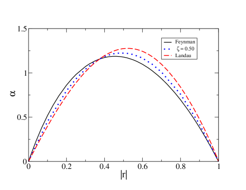
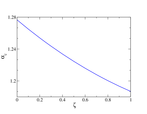
Figure 1: (Color online). Left panel: coupling constant of the fermion-boson system in the chiral limit, Eq. (13), vs. the power $r$ (see Eq. (9)). Solid line: Feynman gauge ($\zeta=1$). Dotted line: $\zeta=0.5$ gauge. Dashed line: Landau gauge ($\zeta=0$). Right panel: the critical value $\alpha_{c}$ of the coupling constant in Eq. (13) for different gauges in the range $0\leq\zeta\leq 1$.

After substituting our Ansatz (9) in Eq. (7), one can show that the condition for a finite integral is $0<r<1$. This solution is not physically acceptable because the LF projection of the scalar function $\phi_{1}$ in the impact-parameter space would have a divergence at the origin (see, e.g., Refs. [43, 44] for a discussion of the BS amplitude in the impact-parameter space for both two-scalar bound system and pion, respectively). On the other hand, for Eq. (8), one realizes that the power $r$ has to fulfill the constraint $-1<r<0$ for getting a well-defined integration on $\gamma^{\prime}$ and avoiding the singularity of the kernel at the end-points (cf. Eq. (10) below).

Therefore, from now on, one can retain only Eq. (8). By performing the integration on $\gamma$ of both sides of Eq. (8), one obtains an integral equation for $f_{2,r}(z)$, and looks for real eigenvalues $\lambda_{2}=2\pi/\alpha$. Namely, one remains with the following integral equation:

$$f_{r}(z)=\frac{\alpha}{2\,\pi}\int_{-1}^{+1}dz^{\prime}\left[{G}(z,z^{\prime})+(1-\zeta){H}(z,z^{\prime})\right]f_{r}(z^{\prime})\,,$$ (10)

where the subscript 2 in $f_{r}(z)$ has been dropped out for simplicity and the two contributions to the kernel are given by

$${G}(z,z^{\prime})=\frac{1}{2\,|r|(1-|r|)}\left[\left(\frac{1+z}{1+z^{\prime}}\right)^{|r|}\,\theta(z^{\prime}-z)+\left(1+\frac{4\,|r|}{(1-z^{\prime})}\right)\left(\frac{1-z}{1-z^{\prime}}\right)^{|r|}\,\,\theta(z-z^{\prime})\right]\,,$$ (11)

and

$$H(z,z^{\prime})=\frac{1}{2\,\,|r|\,(1-|r|)~{}(2-|r|)}\,\Bigg{\{}\left(\frac{1+z}{1+z^{\prime}}\right)^{|r|}~{}\theta(z^{\prime}-z)~{}\Biggl{[}\frac{-|r|^{3}+7\,|r|^{2}-11\,|r|+3}{(3-|r|)}+\frac{|r|\,(1-|r|)}{(1+z^{\prime})}\Biggr{]}$$

$$+\left(\frac{1-z}{1-z^{\prime}}\right)^{|r|}~{}\theta(z-z^{\prime})\Bigg{[}\frac{-|r|^{3}+7\,|r|^{2}-11\,|r|+3}{(3-|r|)}-\frac{|r|(1-2\,|r|)}{(1-z^{\prime})}\Bigg{]}\Bigg{\}}\,.$$ (12)

One can explicitly check that the combination of the factor $(1\pm z)$ with the corresponding theta-function yields a vanishing kernel at the end-points ($z=\pm 1$), implying $f_{r}(\pm 1)=0$. For a finite $r$, the kernel is not symmetric under the transformation $z\leftrightarrow-z$ (this feature entails real and complex conjugated eigenvalues) and therefore we expect that the solutions are non symmetric, i.e. $f_{r}(z)\neq f_{r}(-z)$. Due to this property, it is interesting to observe that in the chiral limit the momentum fraction distributions of the boson and the fermion are distinct, as illustrated in what follows.

By integrating on $z$ both sides of Eq. (10), after inserting the change of variables $y_{\pm}=(1\pm z)/(1\pm z^{\prime})$, one can obtain the following expression of the coupling constant $\alpha$ (see details in Appendix B)

$$\alpha(r,\zeta)=2\pi\,\Biggl{[}{1+2|r|\over|r|(1-r^{2})}+(1-\zeta)\frac{-3\,|r|^{3}+17\,r^{2}-22\,|r|+6}{2\,\,|r|\,(1-r^{2})~{}(2-|r|)(3-|r|)}\Biggr{]}^{-1}.$$ (13)

The coupling constant $\alpha(r,\zeta)$ as a function of the power $r$, for different gauges, is presented in the left panel of Fig. 1. At fixed gauge, $\alpha(r,\zeta)$ grows for increasing $|r|$ up to a maximum value, that we call critical coupling constant, $\alpha_{c}$. The corresponding critical value of $|r|$ is reached around $|r_{c}|\sim 0.5\pm 0.1$ (the uncertainties is given by the variation of $\zeta\in[0,1]$ ). For $\alpha>\alpha_{c}$ the power $r$ becomes complex and Eq. (10) presents a pair of log-periodic solutions, (see, e.g., Ref. [31]), which demands one extra scale to determine the solution uniquely: a phenomenon known as Miransky scaling [21, 22, 23] in the context of quantum field-theory. The critical value $\alpha_{c}$ depends on the covariant gauge, as shown in the right panel of Fig. 1, where the gauge choice has been restricted to the interval $[0,1]$. The value of $\alpha_{c}$ smoothly decreases with respect to $\zeta$ from the Landau to the Feynman gauge, changing by only $\sim 8\%$. The second term in Eq. (13) leads to a decreasing $\alpha_{c}$ for $\zeta\to 1$. The analysis of a more general case with $\zeta\not\in[0,1]$, as well as non covariant gauges, is left for a future work.

It is worth noticing that from the left panel of Fig. 1 one is able not only to separate the region where the solutions Eq. (10) are stable, but also where they are unphysical. This can be understood by recalling that for an increasing value of $\alpha$ the binding grows, and hence the system becomes more compact, i.e. the average size of the system shrinks. The latter feature translates (see Eqs. (14) and (15) below, for a hint) in a tail of the momentum distribution higher, from a heuristic application of the uncertainty principle. This eventually means a smaller value of the power $r$ in Eq. (9). For the branch where $r<r_{c}$, one notices from the left panel of Fig. 1 that the derivative $d\alpha/dr$ is positive, and therefore this region has to be excluded in the analysis of physical systems.

IV Numerical solutions

The solutions of the integral equation for $f_{r}(z)$ have been obtained by expanding $f_{r}(z)$ onto a spline basis. In this way one discretizes the eigenvalue problem, where the coupling constant $\alpha$ is the inverse of the eigenvalue. We solve Eq. (10) looking for the largest real eigenvalue within a set of $r$ values, in different covariant gauges.

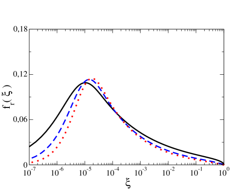
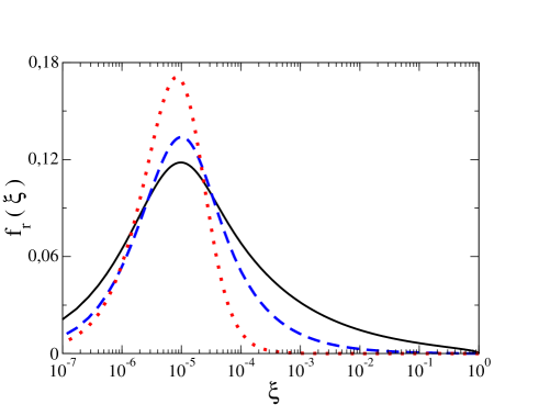
Figure 2: (Color online). $f_{r}(\xi)$ as a function of the momentum fraction $\xi$, for a set of the pair $(|r|,\,\alpha)$ with an arbitrary normalization. Left panel: solutions of Eq. (10) in the Feynman gauge. Solid line: $(|r_{c}|=0.455,\alpha_{c}=1.187)$. Dashed line: $(0.75,0.8248)$. Dotted line: $(0.9999,10^{-4})$. Right panel: the same as in the left panel, but for the Landau gauge. Solid line: $(|r_{c}|=0.522,\alpha_{c}=1.276)$. Dashed line: $(0.75,0.9811)$. Dotted line: $(0.9999,10^{-4})$. Note that $\xi=(1-z)/2$

To analyse the eigenfunctions $f_{r}(z)$ of Eq. (10), it is convenient to use a new variable, $\xi=(1-z)/2$, that corresponds to the fermion longitudinal-momentum fraction. The function $f_{r}(\xi)$ for different values of $|r|$ and $\alpha$ is shown in Fig. 2. In the left panel, the calculation was performed in Feynman gauge, while, in the right panel, it was considered the Landau gauge. For both gauges, $f_{r}(\xi)$ obtained with the pair $(|r_{c}|,\alpha_{c})$ is represented by a solid line. From Fig. 2, one can notice that the general form of $f_{r}(\xi)$ is very similar in different gauges, and it is vanishing at the end-points, as anticipated in the discussion of $f_{r}$ at $z=\pm 1$. In all cases, there is a peak at $\xi\sim 10^{-5}$, which means that the boson average longitudinal-momentum fraction, $\langle 1-\xi\rangle$, is remarkably large. Moreover, the results for the Feynman gauge, $\zeta=1$, are more close each other, while in the Landau gauge, $\zeta=0$, where only the transverse dofs of the vector-boson are present, the differences are more pronounced. The sharpest peak can be obtained in the Landau gauge in correspondence to $r=-1$, i.e. when the NWF fall-off is more fast.

Let us summarize the salient features of $f_{r}(\xi)$: (i) the sharp peak for $\xi$ close to 0 leads to a scalar diquark carrying almost all the mock nucleon longitudinal-momentum fraction; (ii) the Landau-gauge distributions have peaks more sharp than the ones in the Feynman gauge; (iii) in the two gauges, the distributions corresponding to $\alpha_{c}$ are quite similar, given the small dependence of the critical coupling on $\zeta$. Interestingly, the property (i) entails that the massless fermion carries a spin opposite to the mock nucleon one, since for $\xi=0$ the fermion is moving toward negative $z$-axis and the massless fermion helicity is positive (see also details in Ref. [17]). Then, the total spin of the composite state is obtained by adding one unit of orbital angular momentum, which is necessarily of relativistic origin, as expected in the chiral limit.

In the Feynman gauge, where the kernel contribution given in Eq. (11) is acting, the height of the peak close to $\xi=0$ is triggered by the maximum of the kernel contribution that appears for $z\sim z^{\prime}$ (heuristically, one can deduce this feature from the values of the ratios $(1\pm z)/(1\pm z^{\prime})\leq 1$ in combination with the corresponding theta-functions) and by the factor $4\,|r|\,(1-z^{\prime})^{-1}$, which enhances the contribution for $z^{\prime}\to 1$ (recall that $\xi=(1-z)/2$). Analogously, the feature (ii) in the Landau gauge, i.e. the narrowest peak close to $\xi\to 0$ for $|r|>0.5$, can be explained by analysing the kernel contribution given in Eq. (12). The term $-|r|\,(1-2\,|r|)\,(1-z^{\prime})^{-1}$ for $z>z^{\prime}$ in Eq. (12) is additive to the term $1+4|r|(1-z^{\prime})^{-1}$ in Eq. (11) when $|r|>0.5$, enhancing the kernel for $z^{\prime}\to 1$, and consequently resulting in a sharper peak of $f_{r}(\xi)$ in comparison to the Feynman gauge. In this case, one has almost a Dirac delta for $|r|\to 1$ and one can assume a fermion at rest.

IV.1 Transverse degree of freedom

We have quantitatively investigated the relation between what we have learned in the chiral-limit analysis of the BSE and the numerical solutions of the ladder BSE for massive constituents and exchanged vector-boson, Eq. (2), for large transverse momentum, (UV region). In this limit, all the masses can be disregarded with respect to $|\vec{k}_{\perp}|^{2}$ and the scale invariance becomes a very good symmetry. To proceed, let us define the components of the LF-projected BS amplitude [17]

$$\psi_{i}(\gamma,z)=i\,M\int_{-\infty}^{+\infty}dk^{-}\phi_{i}(k,p)$$

$$=\int_{0}^{+\infty}d\gamma^{\prime}\frac{g_{i}(\gamma^{\prime},z)}{\left[\gamma^{\prime}+\gamma+(1-z^{2})\,\kappa^{2}+z^{2}\,\bar{m}^{2}\right]^{2}}\,,$$ (14)

with $\gamma=|\vec{k}_{\perp}|^{2}$. From Eq. (14), with the Ansatz given in Eq. (9), it is possible to conclude that the UV behaviour of the LF-projected BS amplitude is given by (recall that $r\in(-1,0)$)

$$\psi_{2}(\gamma,z)\underset{\gamma\to\infty}{\sim}\gamma^{r-1}\,f_{r}(z)\,.$$ (15)

The strategy to extract relevant information is to solve Eq. (2), for a given set of parameters, and analyze if the solution behaves as predicted by Eq. (15) for large momentum. In the Feynman gauge, the critical value of $\alpha_{c}$ is $1.187$ with the exponent $r_{c}=-0.455$ (see Fig. 1). Therefore, in this gauge, it is expected that the LF-projected BS amplitude corresponding to a coupling constant $\simeq\alpha_{c}$ decreases with $\gamma$, for any $z$, as follows

$$\psi_{2}(\gamma,z)\propto\gamma^{-1.455}\,.$$ (16)

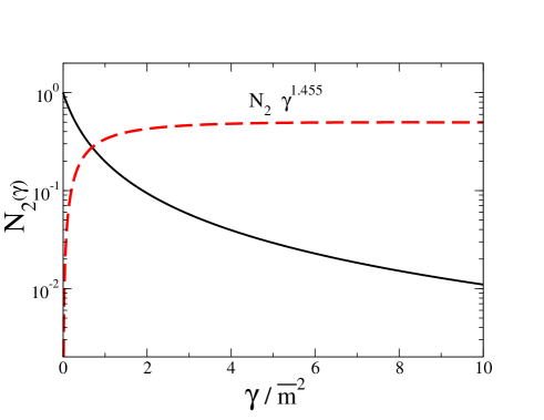
Figure 3: (Color online). The normalized LF amplitude $N_{2}(\gamma)=\psi_{2}(\gamma,\xi_{0}=0.5)/\psi_{2}(0,\xi_{0}=0.5)$ as a function of the transverse momentum square $\gamma=|\vec{k}_{\perp}|^{2}$ in the Feynman gauge, for an equal-mass system, massless vector exchange and binding energy ratio $B/\bar{m}=0.5$. Solid line: $N_{2}(\gamma)$. Dashed line: $N_{2}(\gamma)\times\gamma^{1.455}$, with the power $r_{c}=-0.455$ corresponding to the critical value $\alpha_{c}=1.187$ (cf. Fig. 1, left panel).

In Fig. 3, it is presented the normalized LF-projected BS amplitude

$$N_{2}(\gamma)={\psi_{2}(\gamma,\xi_{0}=0.5)\over\psi_{2}(0,\xi_{0}=0.5)}~{},$$

obtained in Ref. [17], by numerically solving the Minkowski BSE, Eq. (2) for massive constituents, in the Feynman gauge for a massless vector exchange, and equal-mass constituents, $m_{f}=m_{s}$. The binding energy was chosen $B/\bar{m}=0.5$, getting $\alpha=1.189$, that is very close to its critical value. In Fig. 3, the dashed line is the product $N_{2}(\gamma)~{}\gamma^{1-r}$, with $r=-0.455$, and shows a clear asymptotic constant behavior.

In Fig. 4, we present two more comparisons in the Feynman gauge, that correspond to a mock nucleon, with $m_{S}/m_{F}=2$ and $M/\bar{m}=2-B/\bar{m}=1.9$. The massive ladder-BSE is numerically solved in Minkowski space with two different vector-boson masses: $\mu/\bar{m}=0.15$ and $\mu/\bar{m}=0.50$ (see Ref. [17] for details), obtaining $\alpha=0.648$ and $\alpha=0.898$, respectively. For the first value of $\alpha$, one gets $r=-0.817$ from the physical branch of $\alpha(r,\zeta)$ in the left panel of Fig. 1, while for the second value one has $r=-0.718$. In the left panel, the calculation of $N_{2}(\gamma)$, corresponding to $\alpha=0.648$ is shown together with the product $N_{2}(\gamma)~{}\gamma^{1-r}$ and in the right panel there is the comparison with the case $\alpha=0.898$.

Notably, the constant behavior of the dashed lines in Fig. 3 and 4 starts from values of $\gamma/\bar{m}^{2}$ order-of-magnitude different, $\gamma/\bar{m}^{2}>6$ and $\gamma/\bar{m}^{2}>600$, respectively. This is triggered by the difference between the coupling constant and its critical value, as one can realizes from Fig. 3, where $\alpha=\alpha_{c}$ and the scale invariance is established greatly earlier. Moreover, the striking constant behavior of the dashed lines shown in Figs. 3 and 4 illustrates the predictive power of the chiral-limit analysis performed in this work, and suggests the possibility to extract quantitative signatures of the role of the one-particle exchange from the transverse-momentum distributions of hadrons.

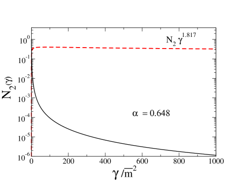
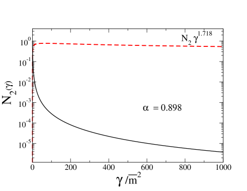
Figure 4: (Color online). The same as in Fig. 3, but with $m_{s}/m_{f}=2$ and binding energy ratio $B/\bar{m}=0.1$ (i.e. $M/\bar{m}=1.9$). Left panel: $\mu/\bar{m}=0.15$ and $\alpha=0.648$. Solid line: $N_{2}(\gamma)$. Dashed line: $N_{2}(\gamma)\times\gamma^{1.817}$. Right panel: $\mu/\bar{m}=0.5$ and $\alpha=0.898$. Solid line: $N_{2}(\gamma)$. Dashed line: $N_{2}(\gamma)\times\gamma^{1.718}$.

IV.2 Longitudinal degree of freedom

The analysis of the function $f_{r}(z)$ close to the end-point $z=-1$, i.e. a longitudinal-momentum fraction $\xi=1$, is interesting for the insight one can gain on the valence parton distribution function, that should dominate the behavior close to $\xi=1$. Restricting to the Feynman gauge, for the sake of simplicity, one has the following approximation of the integral equation in (10) (cf. the kernel in Eq. (11)) for $z\to-1$

$$f_{r}(z)\simeq{\alpha\over 2\pi}~{}{1\over 2|r|(1-|r|)}\Biggl{\{}\epsilon^{|r|}\int_{-1+\epsilon}^{1}dz^{\prime}~{}\Biggl{[}{1\over 1+z^{\prime}}\Biggr{]}^{|r|}f_{r}(z^{\prime})+2^{|r|}\int_{-1}^{-1+\epsilon}dz^{\prime}~{}\Biggl{[}{1\over 1-z^{\prime}}\Biggr{]}^{|r|}\left(1+{4|r|\over(1-z^{\prime})}\right)\Biggr{]}~{}f_{r}(z^{\prime})\Biggr{\}}~{},$$ (17)

that leads to

$$f_{r}(z)\to\epsilon^{|r|}\quad{\rm for}\quad z\to-1+\epsilon~{}~{}.$$ (18)

Notice that the second integral goes to zero more quickly that the first one, since $1>|r|$ and the interval of integration shrinks with the first power of $\epsilon$.

From the above result one deduces that the valence parton distribution function goes to the end-point $\xi=1$ proportionally to $(1-\xi)^{2|r|}$, i.e. $(1-\xi)^{1.634}$ and $(1-\xi)^{1.436}$ for the two cases shown in Fig. 4. It should be recalled that we are considering the chiral limit and a point-like scalar, and that in the limit $\alpha\to 0$ the exponent becomes 2. In general, our $1/2^{+}$ fermion-scalar bound system, in spite of the simple structure adopted, is able to exhibit a large-$\xi$ behavior not too far from the exponent $3$ suggested by the counting rule (see, e.g., Refs. [45, 46, 47, 48] for arguing an acceptable exponent as suggested by the analysis of the proton experimental data).

V Summary

By using the Nakanishi integral representation of the Bethe-Salpeter amplitude, we have solved the homogeneous BSE in the chiral limit for a $1/2^{+}$ bound system, composed by a fermion and a scalar, in Minkowski space. The interaction kernel is given by the one-particle exchange, with the actual dependence upon the different covariant gauges. In the chiral limit, one gets the decoupling of the two-channel integral system that determines the two Nakanishi weight functions, needed for the full reconstruction of the BS amplitude. Moreover, by exploiting the scale invariance that establishes in the chiral limit one gets the factorization of the Nakanishi weight functions in an homogeneous function in $\gamma$ and a function that depends upon the compact variable $z$. Remarkably, the developed formal analysis allows to determine the exact relation between the coupling constant, that drives the binding of the system, and the power that governs the power-like fall-off of the transverse-momentum amplitude, as well as the end-point behavior of the longitudinal momentum fraction amplitude.

Solutions have been presented for Feynman, Landau and covariant gauges in between, where the coupling constant has to be below a critical value in order to allow stable solutions, a problem already known for integral equations having symmetry under scale transformation. Above such critical coupling, the system breaks the continuous scale-invariant regime to a discrete-scale one and the equations allow log-periodic solutions that demand the introduction of a boundary condition. This phenomena is associated with Efimov effect in non-relativistic few-body physics and to the Miransky scaling in the continuum framework of the quantum field-theory (see e.g. [21, 28]). A striking qualitative feature in all analyzed covariant gauges, is that the scalar prefers to carry the nucleon momentum in the spin-antialigned fermion spin opposite to the system one) configuration. Therefore it is necessary to add the fermion-scalar orbital angular momentum to build the mock-nucleon spin, making clear the relativistic origin of such a configuration, already observed in Ref. [17].

Finally, some relevant cases corresponding to both a massless vector-boson exchange and a massive one have been discussed, by comparing in the UV region the solutions of the massive ladder-BSE and the chiral-limit prediction. The very good agreement suggests the interesting role of the hadron transverse-momentum distributions in the search of quantitative signatures of the one-particle exchange, that could be investigated also analyzing the end-point behavior of the valence parton distribution function (as it is well-known from the counting-rule predictions). Plainly, a generalization of the present analysis to the Faddeev-Bethe-Salpeter equations is highly desirable, also including the light-front approach (see, e.g., a first attempt in Ref. [49, 50]), that is necessary for addressing the phenomenology of the hadron momentum distributions.

Appendix A Kernel functions

In this Appendix we present the expressions for the kernel of the integral equations (7) and (8).

$$\mathcal{P}_{1}^{(1)}({\bf V})=-\int_{0}^{1}\,dv\frac{\theta(z^{\prime}-z)\,(1+z)^{-1}\,\left(2-v\right)}{\left[\gamma\,(1-v)\,\left(\frac{1+z^{\prime}}{1+z}\right)+\gamma^{\prime}\right]^{2}}\,.$$

$$\mathcal{P}^{(2)}_{1}({\bf V})=-\frac{1}{2}\int_{0}^{1}dv\Biggl{\{}\frac{(1-v)\,(1+z)^{-1}\,\theta(z^{\prime}-z)}{\left[\gamma\,(1-v)\,\left(\frac{1+z^{\prime}}{1+z}\right)+\gamma^{\prime}\right]^{3}}~{}\left[\frac{(3-5v+2v^{2})(1+z^{\prime})\,\gamma}{(1+z)}+3(1-2v)\,\gamma^{\prime}\right]\,\Biggr{\}}\,.$$ (20)

$$\mathcal{P}_{2}^{(1)}({\bf V})=-\int_{0}^{1}dv\Biggl{\{}\frac{\theta(z^{\prime}-z)}{\gamma\left[]\gamma\,(1-v)\,\left(\frac{1+z^{\prime}}{1+z}\right)+\gamma^{\prime}\right]^{2}}~{}\left[\gamma\,\frac{v(1-v)(1+z^{\prime})}{2(1+z)}+\gamma^{\prime}\,v\right]+\frac{\theta(z-z^{\prime})}{\gamma\left[]\gamma\,(1-v)\,\left(\frac{1-z^{\prime}}{1-z}\right)+\gamma^{\prime}\right]^{2}}$$

$$\times\left[\gamma\,\frac{(1-v)(4+v(1-z^{\prime}))}{2(1-z)}+\gamma^{\prime}\,v\right]\Biggr{\}}\,.$$ (21)

$$\mathcal{P}^{(2)}_{2}({\bf V})=-\frac{1}{2}\int_{0}^{1}(1-v)\,dv\Biggl{\{}\frac{\theta(z^{\prime}-z)}{\gamma\left[\gamma\,(1-v)\,\left(\frac{1+z^{\prime}}{1+z}\right)+\gamma^{\prime}\right]^{3}}~{}\left[\gamma^{2}\,\frac{(1-v)(1+z^{\prime})(1+v^{2}(1+z^{\prime})-v(3+2\,z^{\prime}))}{(1+z)^{2}}\right.$$

$$\left.+\gamma\,\gamma^{\prime}\,\frac{(1-v(2+z^{\prime}))}{(1+z)}+3\,\gamma^{\prime 2}\,v\right]+\frac{v\,\theta(z-z^{\prime})}{\gamma\,\left[\gamma\,(1-v)\,\left(\frac{1-z^{\prime}}{1-z}\right)+\gamma^{\prime}\right]^{3}}\left[-\gamma\,\gamma^{\prime}\,\frac{(4-z^{\prime})}{(1-z)}+3\,\gamma^{\prime 2}\right.$$

$$\left.-\gamma^{2}\,\frac{(1-v)(1-z^{\prime})(1-v-z^{\prime}(2-v))}{(1-z)^{2}}\right]\,\Biggr{\}}\,$$ (22)

with ${\bf V}\equiv\{\gamma,z,\gamma^{\prime},z^{\prime}\}$.

Appendix B Coupling constant $\alpha$ and power $r$

This Appendix illustrates the formal steps to obtain the relation between the coupling constant $\alpha$ and the power $r$. The basic step is the integration on the variable $z$ of both sides in Eq. (10). In particular, to perform the integration on the two kernel contribution in Eqs. (11) and (12), respectively, the following result is useful

$$\int_{-1}^{+1}dz\,\left({1\pm z\over 1\pm z^{\prime}}\right)^{|r|}\,\theta(\pm z^{\prime}\mp z)=\left(1\pm z^{\prime}\right)\,\int_{0}^{2/(1\pm z^{\prime})}dy_{\pm}\,y_{\pm}^{|r|}\,\theta(1-y_{\pm})=\,\left(1\pm z^{\prime}\right)\int_{0}^{1}dy_{\pm}\,y_{\pm}^{|r|}={1\pm z^{\prime}\over 1+|r|}~{}~{},$$ (23)

with $y_{\pm}=(1\pm z)/(1\pm z^{\prime})$. Then, one gets

$$\int_{-1}^{+1}G(z,z^{\prime})\,dz={1\over 2|r|(1-|r|)}\left[{1+z^{\prime}\over 1+|r|}+\left(1+{4|r|\over 1-z^{\prime}}\right){1-z^{\prime}\over 1+|r|}\right]={1+2|r|\over|r|(1-r^{2})}~{},$$ (24)

and

$$\int_{-1}^{+1}H(z,z^{\prime})\,dz=\frac{1}{2|r|(1-r^{2})~{}(2-|r|)}~{}\Bigg{[}2\frac{-|r|^{3}+7\,|r|^{2}-11\,|r|+3}{(3-|r|)}+r^{2}\Bigg{]}=\frac{-3\,|r|^{3}+17\,|r|^{2}-22\,|r|+6}{2|r|(1-r^{2})~{}(2-|r|)(3-|r|)}\,.$$ (25)

Collecting the above result, from Eq. (10) one gets

$$C_{0}=\int_{-1}^{+1}dz~{}f_{r}(z)=\frac{\alpha}{2\,\pi}\int_{-1}^{+1}dz^{\prime}\int_{-1}^{+1}dz~{}\Bigl{[}{G}(z,z^{\prime})+(1-\zeta){H}(z,z^{\prime})\Bigr{]}\,f_{r}(z^{\prime})$$

$$=\frac{\alpha}{2\,\pi}\Biggl{[}{1+2|r|\over|r|(1-r^{2})}+(1-\zeta)\frac{-3\,|r|^{3}+17\,|r|^{2}-22\,|r|+6}{2\,\,|r|\,(1-r^{2})~{}(2-|r|)(3-|r|)}\Biggr{]}\,\int_{-1}^{+1}dz^{\prime}f_{r}(z^{\prime})\,,$$ (26)

and therefore

$$\alpha=2\pi\,\Biggl{[}{1+2|r|\over|r|(1-r^{2})}+(1-\zeta)\frac{-3\,|r|^{3}+17\,r^{2}-22\,|r|+6}{2\,\,|r|\,(1-r^{2})~{}(2-|r|)(3-|r|)}\Biggr{]}^{-1}.$$ (27)

References

- [1] M. Constantinou, A. Courtoy, M. A. Ebert, M. Engelhardt, T. Giani, T. Hobbs, T. J. Hou, A. Kusina, K. Kutak and J. Liang, et al. “Parton distributions and lattice-QCD calculations: Toward 3D structure,” Prog. Part. Nucl. Phys. 121, 103908 (2021) doi:10.1016/j.ppnp.2021.103908 [arXiv:2006.08636 [hep-ph]].
- [2] C. Egerer et al. [HadStruc], “Transversity parton distribution function of the nucleon using the pseudodistribution approach,” Phys. Rev. D 105, no.3, 034507 (2022) doi:10.1103/PhysRevD.105.034507 [arXiv:2111.01808 [hep-lat]].
- [3] X. Ji, “Large-Momentum Effective Theory vs. Short-Distance Operator Expansion: Contrast and Complementarity,” [arXiv:2209.09332 [hep-lat]].
- [4] C. D. Roberts, D. G. Richards, T. Horn and L. Chang, “Insights into the emergence of mass from studies of pion and kaon structure,” Prog. Part. Nucl. Phys. 120, 103883 (2021) doi:10.1016/j.ppnp.2021.103883 [arXiv:2102.01765 [hep-ph]].
- [5] R. Abdul Khalek, A. Accardi, J. Adam, D. Adamiak, W. Akers, M. Albaladejo, A. Al-bataineh, M. G. Alexeev, F. Ameli and P. Antonioli, et al. “Science Requirements and Detector Concepts for the Electron-Ion Collider: EIC Yellow Report,” Nucl. Phys. A 1026, 122447 (2022) doi:10.1016/j.nuclphysa.2022.122447 [arXiv:2103.05419 [physics.ins-det]].
- [6] D. P. Anderle, V. Bertone, X. Cao, L. Chang, N. Chang, G. Chen, X. Chen, Z. Chen, Z. Cui and L. Dai, et al. “Electron-ion collider in China,” Front. Phys. (Beijing) 16, no.6, 64701 (2021) doi:10.1007/s11467-021-1062-0 [arXiv:2102.09222 [nucl-ex]].
- [7] R. Alkofer and L. von Smekal, “The Infrared behavior of QCD Green’s functions: Confinement dynamical symmetry breaking, and hadrons as relativistic bound states,” Phys. Rept. 353, 281 (2001) doi:10.1016/S0370-1573(01)00010-2 [arXiv:hep-ph/0007355 [hep-ph]].
- [8] G. Eichmann, H. Sanchis-Alepuz, R. Williams, R. Alkofer and C. S. Fischer, “Baryons as relativistic three-quark bound states,” Prog. Part. Nucl. Phys. 91, 1-100 (2016) doi:10.1016/j.ppnp.2016.07.001 [arXiv:1606.09602 [hep-ph]].
- [9] M. Y. Barabanov, M. A. Bedolla, W. K. Brooks, G. D. Cates, C. Chen, Y. Chen, E. Cisbani, M. Ding, G. Eichmann and R. Ent, et al. “Diquark correlations in hadron physics: Origin, impact and evidence,” Prog. Part. Nucl. Phys. 116, 103835 (2021) doi:10.1016/j.ppnp.2020.103835 [arXiv:2008.07630 [hep-ph]].
- [10] C. Alexandrou, P. de Forcrand and B. Lucini, “Evidence for diquarks in lattice QCD,” Phys. Rev. Lett. 97, 222002 (2006) doi:10.1103/PhysRevLett.97.222002 [arXiv:hep-lat/0609004 [hep-lat]].
- [11] T. DeGrand, Z. Liu and S. Schaefer, “Diquark effects in light baryon correlators from lattice QCD,” Phys. Rev. D 77, 034505 (2008) doi:10.1103/PhysRevD.77.034505 [arXiv:0712.0254 [hep-ph]].
- [12] R. Babich, N. Garron, C. Hoelbling, J. Howard, L. Lellouch and C. Rebbi, “Diquark correlations in baryons on the lattice with overlap quarks,” Phys. Rev. D 76, 074021 (2007) doi:10.1103/PhysRevD.76.074021 [arXiv:hep-lat/0701023 [hep-lat]].
- [13] Y. Bi, H. Cai, Y. Chen, M. Gong, Z. Liu, H. X. Qiao and Y. B. Yang, “Diquark mass differences from unquenched lattice QCD,” Chin. Phys. C 40, no.7, 073106 (2016) doi:10.1088/1674-1137/40/7/073106 [arXiv:1510.07354 [hep-ph]].
- [14] A. Francis, P. de Forcrand, R. Lewis and K. Maltman, “Diquark properties from full QCD lattice simulations,” JHEP 05, 062 (2022) doi:10.1007/JHEP05(2022)062 [arXiv:2106.09080 [hep-lat]].
- [15] K. Watanabe and N. Ishii, “Building Diquark Model from Lattice QCD,” Few Body Syst. 62, no.3, 45 (2021) doi:10.1007/s00601-021-01627-y [arXiv:2105.07969 [hep-lat]].
- [16] K. Watanabe, “Quark-diquark potential and diquark mass from lattice QCD,” Phys. Rev. D 105, no.7, 074510 (2022) doi:10.1103/PhysRevD.105.074510 [arXiv:2111.15167 [hep-lat]].
- [17] J. H. Alvarenga Nogueira, D. Colasante, V. Gherardi, T. Frederico, E. Pace and G. Salmè, “Solving the Bethe-Salpeter Equation in Minkowski Space for a Fermion-Scalar system,” Phys. Rev. D 100, no.1, 016021 (2019) doi:10.1103/PhysRevD.100.016021 [arXiv:1907.03079 [hep-ph]].
- [18] N. Nakanishi, “Partial-Wave Bethe-Salpeter Equation,” Phys. Rev. 130, 1230-1235 (1963) doi:10.1103/PhysRev.130.1230.
- [19] N. Nakanishi, “Graph Theory and Feynman Integrals,” (Gordon and Breach, New York, 1971).
- [20] D. Dudal, O. Oliveira and P. J. Silva, “Källén-Lehmann spectroscopy for (un)physical degrees of freedom,” Phys. Rev. D 89, no.1, 014010 (2014) doi:10.1103/PhysRevD.89.014010 [arXiv:1310.4069 [hep-lat]].
- [21] V. A. Miransky, “Dynamics of Spontaneous Chiral Symmetry Breaking and Continuum Limit in Quantum Electrodynamics,” Nuovo Cim. A 90, 149-170 (1985) doi:10.1007/BF02724229
- [22] V. A. Miransky and K. Yamawaki, “Conformal phase transition in gauge theories,” Phys. Rev. D 55, 5051-5066 (1997) [erratum: Phys. Rev. D 56, 3768 (1997)] doi:10.1103/PhysRevD.56.3768 [arXiv:hep-th/9611142 [hep-th]].
- [23] V. A. Miransky, “Conformal phase transition, beta function, and infrared dynamics in QCD,” [arXiv:hep-ph/0003137 [hep-ph]].
- [24] S. M. Dorkin, M. Beyer, S. S. Semikh and L. P. Kaptari, “Two-Fermion Bound States within the Bethe-Salpeter Approach,” Few Body Syst. 42, 1-32 (2008) doi:10.1007/s00601-008-0196-8 [arXiv:0708.2146 [nucl-th]].
- [25] M. Mangin-Brinet, J. Carbonell and V. A. Karmanov, “Stability of bound states in the light front Yukawa model,” Phys. Rev. D 64, 027701 (2001) doi:10.1103/PhysRevD.64.027701 [arXiv:hep-th/0102068 [hep-th]].
- [26] M. Mangin-Brinet, J. Carbonell and V. A. Karmanov, “Relativistic bound states in Yukawa model,” Phys. Rev. D 64, 125005 (2001) doi:10.1103/PhysRevD.64.125005 [arXiv:hep-th/0107235 [hep-th]].
- [27] J. Carbonell and V. A. Karmanov, Eur. Phys. J. A 46, 387-397 (2010) doi:10.1140/epja/i2010-11055-4 [arXiv:1010.4640 [hep-ph]].
- [28] D. B. Kaplan, J. W. Lee, D. T. Son and M. A. Stephanov, “Conformality Lost,” Phys. Rev. D 80, 125005 (2009) doi:10.1103/PhysRevD.80.125005 [arXiv:0905.4752 [hep-th]].
- [29] T. Enss, R. Haussmann and W. Zwerger, “Viscosity and scale invariance in the unitary Fermi gas,” Annals Phys. 326, 770-796 (2011) doi:10.1016/j.aop.2010.10.002 [arXiv:1008.0007 [cond-mat.quant-gas]].
- [30] Y. Nakayama, “Scale invariance vs conformal invariance,” Phys. Rept. 569, 1-93 (2015) doi:10.1016/j.physrep.2014.12.003 [arXiv:1302.0884 [hep-th]].
- [31] L. Landau, Lifshitz, “Non-relativistic theory quantum me- chanics,” translated from the russian by jb sykes and js bell (1958).
- [32] L. H. Thomas, “The Interaction Between a Neutron and a Proton and the Structure of H**3,” Phys. Rev. 47, 903-909 (1935) doi:10.1103/PhysRev.47.903
- [33] V. Efimov, “Energy levels arising from resonant two-body forces in a three-body system,” Phys. Lett. B 33, 8, 563-564 (1970) 10.1016/0370-2693(70)90349-7.
- [34] V. Efimov, “Qualitative treatment of three-nucleon properties,” Nuc. Phys. A 362, 1, 45-70 (1981) 10.1016/0375-9474(81)90669-2.
- [35] T. Frederico, A. Delfino, L. Tomio and M. T. Yamashita, “Universal aspects of light halo nuclei,” Prog. Part. Nucl. Phys. 67, 939-994 (2012) doi:10.1016/j.ppnp.2012.06.001.
- [36] W. de Paula, T. Frederico, G. Salmè and M. Viviani, “Advances in solving the two-fermion homogeneous Bethe-Salpeter equation in Minkowski space,” Phys. Rev. D 94, no.7, 071901 (2016) doi:10.1103/PhysRevD.94.071901 [arXiv:1609.00868 [hep-th]].
- [37] W. de Paula, T. Frederico, G. Salmè, M. Viviani and R. Pimentel, “Fermionic bound states in Minkowski-space: Light-cone singularities and structure,” Eur. Phys. J. C 77, no.11, 764 (2017) doi:10.1140/epjc/s10052-017-5351-2 [arXiv:1707.06946 [hep-ph]].
- [38] W. de Paula, E. Ydrefors, J. H. Nogueira Alvarenga, T. Frederico and G. Salmè, “Parton distribution function in a pion with Minkowskian dynamics,” Phys. Rev. D 105, no.7, L071505 (2022) doi:10.1103/PhysRevD.105.L071505 [arXiv:2203.07106 [hep-ph]].
- [39] E. Ydrefors, W. de Paula, J. H. A. Nogueira, T. Frederico and G. Salmé, “Pion electromagnetic form factor with Minkowskian dynamics,” Phys. Lett. B 820, 136494 (2021) doi:10.1016/j.physletb.2021.136494 [arXiv:2106.10018 [hep-ph]].
- [40] F. E. Clos, “On the Scale Invariance of certain Complex Systems,” Doctoral Thesis, Universitat Autonoma de Barcelona, (2015).
- [41] W. De Paula, A. Delfino, T. Frederico and L. Tomio, “Limit cycles in the spectra of mass imbalanced many-boson system,” J. Phys. B 53, no.20, 205301 (2020) doi:10.1088/1361-6455/aba9e2 [arXiv:1903.10321 [quant-ph]].
- [42] F. E. Clos, “Fractals in the Physical Sciences,” Nonlinear science: theory and applications (Manchester University Press, 1990).
- [43] C. Gutierrez, V. Gigante, T. Frederico, G. Salmè, M. Viviani and L. Tomio, “Bethe–Salpeter bound-state structure in Minkowski space,” Phys. Lett. B 759, 131-137 (2016) doi:10.1016/j.physletb.2016.05.066 [arXiv:1605.08837 [hep-ph]].
- [44] W. de Paula, E. Ydrefors, J. H. Alvarenga Nogueira, T. Frederico and G. Salmè, “Observing the Minkowskian dynamics of the pion on the null-plane,” Phys. Rev. D 103, no.1, 014002 (2021) doi:10.1103/PhysRevD.103.014002 [arXiv:2012.04973 [hep-ph]].
- [45] R. D. Ball, E. R. Nocera and J. Rojo, “The asymptotic behaviour of parton distributions at small and large ,” Eur. Phys. J. C 76, no.7, 383 (2016) doi:10.1140/epjc/s10052-016-4240-4 [arXiv:1604.00024 [hep-ph]].
- [46] A. Accardi, L. T. Brady, W. Melnitchouk, J. F. Owens and N. Sato, “Constraints on large- parton distributions from new weak boson production and deep-inelastic scattering data,” Phys. Rev. D 93, no.11, 114017 (2016) doi:10.1103/PhysRevD.93.114017 [arXiv:1602.03154 [hep-ph]].
- [47] M. Bonvini and F. Giuli, “A new simple PDF parametrization: improved description of the HERA data,” Eur. Phys. J. Plus 134, no.10, 531 (2019) doi:10.1140/epjp/i2019-12872-x [arXiv:1902.11125 [hep-ph]].
- [48] T. J. Hou, J. Gao, T. J. Hobbs, K. Xie, S. Dulat, M. Guzzi, J. Huston, P. Nadolsky, J. Pumplin and C. Schmidt, et al. “New CTEQ global analysis of quantum chromodynamics with high-precision data from the LHC,” Phys. Rev. D 103, no.1, 014013 (2021) doi:10.1103/PhysRevD.103.014013 [arXiv:1912.10053 [hep-ph]].
- [49] E. Ydrefors and T. Frederico, “Proton image and momentum distributions from light-front dynamics,” Phys. Rev. D 104, no.11, 114012 (2021) doi:10.1103/PhysRevD.104.114012 [arXiv:2108.02146 [hep-ph]].
- [50] E. Ydrefors and T. Frederico, “Proton quark distributions from a light-front Faddeev-Bethe-Salpeter approach,” Phys. Lett. B 838, 137732 (2023) doi:10.1016/j.physletb.2023.137732 [arXiv:2211.10959 [hep-ph]].