Splitting physics-informed neural networks for inferring the dynamics of integer- and fractional-order neuron models

Abstract

We introduce a new approach for solving forward systems of differential equations using a combination of splitting methods and physics-informed neural networks (PINNs). The proposed method, splitting PINN, effectively addresses the challenge of applying PINNs to forward dynamical systems and demonstrates improved accuracy through its application to neuron models. Specifically, we apply operator splitting to decompose the original neuron model into sub-problems that are then solved using PINNs. Moreover, we develop an $L^{1}$ scheme for discretizing fractional derivatives in fractional neuron models, leading to improved accuracy and efficiency. The results of this study highlight the potential of splitting PINNs in solving both integer- and fractional-order neuron models, as well as other similar systems in computational science and engineering.

92B20, 34C28, 37M05, 34A08

1 Introduction

The human brain is a complex system that involves the interactions of billions of neurons. Mathematical models can be used to simulate the neuronal activity in the brain as a system of differential equations, allowing researchers to better understand how the brain works. Studies related to spiking neurons are performed numerically or biophysically. In numerical studies, the main goal is to solve neural equations and investigate how the dynamic behavior changes for different inputs. Biophysical approaches focus on interpreting the dynamic behavior of spiking neurons according to available experimental observations [2, 58].

Another interesting aspect of spiking neuron models is that they can be formulated as fractional-order equations, which take into account long-term memory. The order of the derivative in these equations can affect the neuron’s response [54, 59, 63], making this an important area of research. Recent works in both integer- and fractional-order neuron models are discussed in Section 3.3.

In this work we introduce a new approach for solving neuron models that combines operator splitting methods with physics-informed neural networks (PINNs). Operator splitting methods have been successfully applied in various fields of physics and engineering [18, 15, 52, 11, 51, 6, 34, 23], while PINNs provide a powerful tool for approximating the solution of differential equations. A general introduction to the splitting method can be found in [43, 25].

PINNs were first introduced by Raissi et al. [50]. In this method, the solution of a differential equation is approximated using a neural network, and the parameters of the network are determined by solving a minimization problem that includes residual functions at collocation points, as well as initial and boundary conditions.

PINNs have been applied successfully to a broad range of ordinary and partial differential equations, including fractional equations [48], integro-differential equations, stochastic partial differential equations [68], and inverse problems [44]. There have also been several extensions to the original PINN, such as Fractional PINN (FPINN) [48], physics-constrained neural networks (PCNN) [36, 69], variable hp-VPINN [30], conservative PINN (CPINN) [29], Bayesian PINN [66], parallel PINN [55], Self-Adaptive PINN [42], and Physics informed Adversarial training (PIAT) [53]. Innovations in activation functions, gradient optimization techniques, neural network structures, and loss function structures have driven recent advances in the field. Despite these advances, improvements are still possible, especially concerning unresolved theoretical and practical issues.

Our study makes two important contributions to the field of neural modeling. First, we propose a new method, called the splitting PINN, that employs the operator splitting technique to decompose the original spiking neuron model into sub-problems, which are then solved using PINNs. We demonstrate the effectiveness and accuracy of this method by applying it to integer- and fractional-order neuron models with oscillatory responses, for which vanilla PINN and FPINN formulations fail to predict the solutions. Second, we introduce a novel $L^{1}$-scheme for discretizing fractional derivatives in fractional neuron models, which leads to improved accuracy and efficiency in solving these complex models. Our results show that the combination of the splitting PINN method and the $L^{1}$-scheme accurately solves fractional neuron models and provides valuable insights into the underlying mechanisms of neural activity.

This paper is organized as follows: Section 2 provides an overview of the proposed method for a given system of differential equations. Section 3 introduces various neuron models and their properties, including the Leaky Integrate-and-Fire (LIF), Izhikevich, Hodgkin-Huxley (HH), and the fractional order Hodgkin-Huxley (FO-HH) models. The efficiency and accuracy of splitting PINNs and FPINNs are demonstrated in Section 4 by applying our algorithm to different neuron models. Finally, we present a discussion of the main results in Section 5. The results and conclusion of this paper will provide valuable insights into the potential of this new approach for solving neuron models and other similar systems in computational science and engineering.

2 Problem setup and solution methodology

Let us consider the general form of a nonlinear system of differential equations as follows,

$$\frac{dx_{i}}{dt}=f_{i}(t,x),\qquad i=1,\cdots,n,\qquad t\in[0,T].$$ (1)

Before introducing the splitting PINN for solving the given systems of differential equations, we briefly review what splitting methods are, in general.

2.1 Splitting method

For solving the given system (1), let us rewrite it as follows,

$$\frac{dx}{dt}=f(t,x(t)),\qquad x(0)=x_{0}\qquad x\in\mathbb{R}^{n},$$

then by using splitting method, $x$ is decomposed into $(x^{*},x^{**})$, where $x^{*},x^{**}\in\mathbb{R}^{d}\ (d<n)$. So, we have

$$\frac{dx^{*}}{dt}=f(t,x^{*}(t)),\qquad x^{*}(0)=x^{*}_{0},$$ (2)

$$\frac{dx^{**}}{dt}=f(t,x^{**}(t)),\qquad x^{**}(0)=x^{**}_{0},$$ (3)

and $x^{*}_{0}$ and $x^{**}_{0}$ are the given vectors of initial conditions. After solving the above sub-systems by the given practical algorithms, we denote the solutions of (2) and (3) as

$$\phi_{\Delta t}^{(*)}x^{*}_{0}\qquad\mathrm{and}\qquad\phi_{\Delta t}^{(**)}x^{**}_{0},$$

where $\phi_{\Delta t}^{(*)}$ and $\phi_{\Delta t}^{(**)}$ are $x^{*}$-flow and $x^{**}$-flow, respectively, and ${\Delta t}$ is the step size. Then, by combining the solutions of sub-systems, the approximation operator in $x$-flow can be written as follows

$$\phi_{\Delta t}^{(*)}\circ\phi_{\Delta t}^{(**)}\qquad\mbox{or}\qquad\phi_{{\Delta t}/2}^{(**)}\circ\phi_{\Delta t}^{(*)}\circ\phi_{{\Delta t}/2}^{(**)}$$ (4)

and $\phi_{\Delta t}^{(*)}$ and $\phi_{\Delta t}^{(**)}$ are interchangable. The first splitting is the Lie-splitting method [62], which is first-order, and the second is the Strang splitting method [56], which is a second-order method.

On interval $[0,T]$, we first split the original system into sub-systems (sub-problems) for each sub-interval $[t^{j},t^{j+1}]\ (j=0,1,\cdots,J-1,\ t^{J}=T)$. Then the solution of the original system at time $t^{j+1}$ can be approximated as follows

$$x(t^{j+1})=\phi_{\Delta t}^{(*)}\circ\phi_{\Delta t}^{(**)}x(t^{j})$$

where $x(t^{j})$ is the accurate solution at $t=t^{j}$.

2.2 Physics informed neural network

Consider an initial value problem as follows,

$$\begin{split}\frac{dx}{dt}&=f(t,x(t)),\qquad x\in\Omega\subseteq\mathbb{R}^{n},\ t\in[0,T],\\ x(0)&=x_{0},\end{split}$$ (5)

where $f$ is a nonlinear differential operator, and $x$ is the unknown solution with known initial condition.

By using the PINN framework, the solution of the above equation is approximated by a fully connected neural network $\mathcal{N}^{L}$ with $L$ layers and $N$ neurons, where the output of $l$-th hidden layer is defined as follows

$$\mathcal{N}^{l}(t)=W^{l}\sigma(\mathcal{N}^{l-1}(t))+b^{l},\qquad 2\leq l\leq L,$$ (6)

$t\in\mathbb{R}$ is the input vector, $\sigma(\cdot)$ is the activation function, $\sigma(\mathcal{N}^{l-1}(t))\in\mathbb{R}^{N}$ $\{W^{l}\in\mathbb{R}^{N\times N},b^{l}\in\mathbb{R}^{N}\}$ are the network parameters, $\mathcal{N}^{1}(t)=W^{1}t+b^{1}$ and $\mathcal{N}^{L}(t)$ is the output of the last layer which is used to approximate the solution. The unknown parameters can be learned by solving a minimization problem that consists of the residual error terms as follows

$$\min_{w,b}\qquad\frac{1}{N_{r}}\sum_{i=1}^{N_{r}}|\frac{dx}{dt}(t^{i})-f(t^{i},x(t^{i}))|^{2}+|x(0)-x_{0}|^{2},$$ (7)

where $N_{r}$ is the number of collocation points. The parameters are randomly initialized and optimized, and then the approximate solution is obtained.

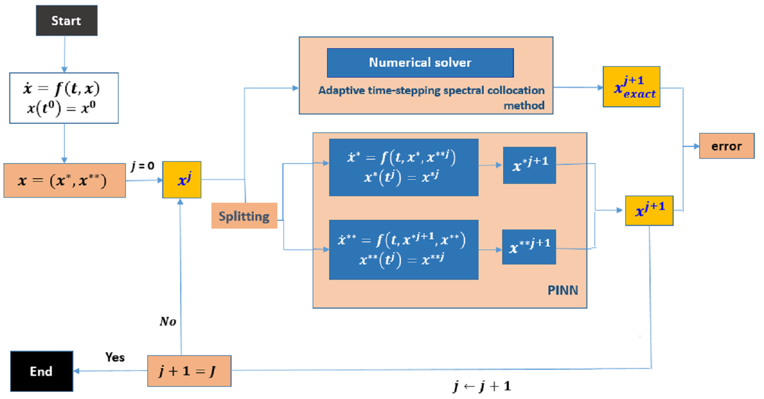
Figure 1: Overview of the Splitting PINN : We first split the original system into sub-systems (sub-problems) for each sub-interval $[t^{j},t^{j+1}]$. For each sub-interval, $x(t^{j})$ is known, the sub-systems are solved using PINN and then the solutions are combined to obtain the approximate solution $x(t^{j+1})$. To evaluate the error, we obtain the reference solution, $x_{exact}(t^{j+1})$, by using a high-order numerical solver (for more details, see Appendix B). The algorithm proceeds until arriving at a given accuracy for each sub-interval.

The framework uses automatic differentiation to calculate the derivatives of the solution, which eliminates the need for manual calculation or numerical discretization [5]. This capability is available in popular deep-learning frameworks such as TensorFlow and PyTorch.

3 Neuron models

Until now, various neuron models have been presented for the biological simulations of different parts of the brain. Among them, we can mention the leaky integrate-and-fire (LIF) model, the Izhikevich model, the Hodgkin-Huxley (HH) model, and FitzHugh-Nagumo (FHN) model, which model the membrane behavior [2]. These models can be classified into integer-and fractional-order models. Integer-order models can capture complex phenomena in the neuron system. However, they represent only one type of firing characteristic for constant parameters of the model. On the other hand, fractional-order models can sexhibit different dynamic behavior of neurons for constant parameters [58]. This makes fractional-order models more versatile and capable of capturing a wider range of neuron behavior.

3.1 Neuron models: integer order

3.1.1 IF and LIF models

The neuron model of integrate-and-fire (IF model) is one of the best models due to the simplicity of calculations and closeness to human biological conditions. This model is a simplified version of the HH model, which is described by an equation and an assumption. Unlike the HH model, the IF model does not automatically generate an action potential. This model can be determined by

$$C_{m}\frac{dV}{dt}=I(t),$$ (8)

with the following spike condition: if $V=V_{th}$, a spike at $t_{spike}$ is generated and the membrane potential $V(t)$ is set to $V_{rest}$ for a refractory period $\tau_{ref}$ [20, 21]. $C_{m}$ is the membrane capacitance, $V_{th}$ is the voltage threshold and $V_{rest}$ is the resting membrane potential.

A generalized type of IF model is the leaky integrate-and-fire (LIF) model, which adds a leak to the membrane potential. This model is defined by the following equation,

$$\tau\frac{dV}{dt}=-(V-V_{rest})+RI(t),$$ (9)

where $\tau=RC_{m}$ is the membrane time constant and $R$ is the membrane resistance. Because of the important properties of this model, like its computational simplicity [27], accuracy in terms of the spiking behavior and spike times of neurons, and simulating speed [10, 39], this model has become one of the most popular and advantageous neuron models in neuromorphic computing [1, 7, 45, 39]. Also, the characteristic of membrane potential decay over time can be seen in the LIF model.

More complex types of IF models include exponential integrate-and-fire, quadratic integrate-and-fire, and adaptive exponential integrate-and-fire [8].

3.1.2 Izhikevich model

Another neuron model for simulating the membrane behavior is the Izhikevich model. Two important features of this model are computational efficiency and biological plausibility. It reduces the more complex Hodgkin-Huxley model to a 2D system of ordinary differential equations of the form

$$\begin{split}&\frac{dv}{dt}=0.04v^{2}+5v+140-u+I(t),\\ &\frac{du}{dt}=a(bv-u),\end{split}$$ (10)

with the auxiliary condition

$$\mbox{if}\ v\geq v_{th},\ \mbox{then}\left\{\begin{array}[]{l}v\leftarrow c\\ u\leftarrow u+d\end{array}\right\}$$ (11)

with $u$ and $v$ being dimensionless variables. The variable $v$ is the membrane potential of the neuron, and $u$ is the membrane recovery variable, which accounts for the activation of the $K^{+}$ ion current and the inactivation of the $Na^{+}$ ion current and provides negative feedback to the membrane potential. The dimensionless parameters $a$, $b$, $c$, and $d$ regulate the behavior of the neuron.

The auxiliary condition (11) triggers a reset of the neuron when the membrane potential surpasses the threshold, simulating a spike. This model is capable of reproducing the spiking and bursting behavior of neurons in real-time, making it a widely used model in simulations of large-scale neural networks.

3.1.3 Hodgkin-Huxley model

From a biophysical perspective, the nerve cell’s action potential is generated by the flow of ions through the cell membrane’s ion channels. Hodgkin and Huxley described the dynamics of these membrane currents through a set of coupled differential equations based on their experiments on the giant squid axon [24].

The mechanism of the action potential can be understood with reference to Figure 2. A capacitor, resistor, and transistor were used to simulate the equivalent circuit. Changes in the action potential were observed by applying the current $I(t)$ and adjusting the capacitance and leakage resistance of the sodium and potassium channels.

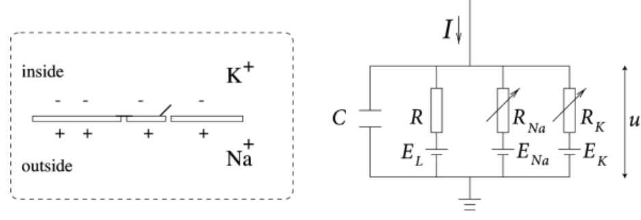
Figure 2: Schematic diagram for the Hodgkin-Huxley model [24]. Left: ion channels on the membrane of the neuron. Right: simulated circuit with $I$ denoting the input current.

The circuit of the Hodgkin-Huxley (HH) model consists of four parallel branches: integrative branch, leaky branch, $K^{+}$ channel, and $Na^{+}$ channel. A system of four coupled differential equations was used to describe the membrane potential of a giant squid axon as follows

$$\begin{split}\frac{dV_{m}}{dt}=&F_{1}(t,V_{m},n,m,h),\qquad\frac{dn}{dt}=F_{2}(t,V_{m},n,m,h),\\ \frac{dm}{dt}=&F_{3}(t,V_{m},n,m,h),\qquad\frac{dh}{dt}=F_{4}(t,V_{m},n,m,h),\end{split}$$ (12)

where

$$\begin{split}&F_{1}=\frac{1}{C_{m}}(-g_{L}(V_{m}-E_{L})-g_{K}n^{4}(V_{m}-E_{K})-g_{Na}m^{3}h(V_{m}-E_{Na})+I(t)),\\ &F_{2}=\alpha_{n}(V_{m}(t))(1-n(t))-\beta_{n}(V_{m}(t))n,\\ &F_{3}=\alpha_{m}(V_{m}(t))(1-m(t))-\beta_{m}(V_{m}(t))m,\\ &F_{4}=\alpha_{h}(V_{m}(t))(1-h(t))-\beta_{h}(V_{m}(t))h,\end{split}$$ (13)

and $g_{Na}$, $g_{K}$ and $g_{L}$ are the maximum conductances of the $Na^{+}$, $K^{+}$ and leak currents. The variables $\alpha_{x}$ and $\beta_{x}$ of the current channel conductances are dependent functions of $V_{m}(t)$ as follows:

$$\begin{split}&\alpha_{n}(V_{m})=\frac{0.1-0.01(V_{m}-V_{0})}{e^{1-0.1(V_{m}-V_{0})}-1},\qquad\beta_{n}(V_{m})=0.125e^{-(V_{m}-V_{0})/80},\\ &\alpha_{m}(V_{m})=\frac{2.5-0.1(V_{m}-V_{0})}{e^{2.5-0.1(V_{m}-V_{0})}-1},\qquad\beta_{m}(V_{m})=4.0e^{-(V_{m}-V_{0})/80},\\ &\alpha_{h}(V_{m})=0.07e^{-(V_{m}-V_{0})/20},\qquad\ \ \ \ \beta_{h}(V_{m})=\frac{1}{1+e^{3-0.1(V_{m}-V_{0})}}.\end{split}$$ (14)

3.2 Neuron models: fractional order

In recent years, fractional differential equations have been developed to improve the modeling of many biological phenomena, including mechanical properties of viscoelastic tissue [40], the tissue-electrode interface [41], pharmacokinetics of drug delivery and absorption [13, 14, 49], and anomalous calcium sub-diffusion in micro-domains [57].

The main characteristic of using fractional derivatives is their non-locality. This means that the next state of the system depends on the current state and all historical states before it. This advantage makes the study of fractional order systems an active area of research.

3.2.1 Fractional derivative definitions

In this Section, we present the definitions of fractional derivatives. There are different methods for defining fractional derivatives, among which we can mention the Grünwald–Letnikov derivative, Riemann–Liouville derivative, and Caputo derivative [33]. The models in this paper are defined using the Caputo fractional derivative.

Definition 1.

The Caputo fractional derivative of the function $f(t)$ with order $\alpha>0$ is defined as

$$\ _{C}D^{\alpha}_{a,t}f(t)=\frac{1}{\Gamma(n-\alpha)}\int_{a}^{t}(t-s)^{n-\alpha-1}f^{(n)}(s)ds,$$ (15)

where $n-1<\alpha<n$ and $n$ in a non-negative integer.

If $a=0$, then we can use $\frac{d^{\alpha}}{dt^{\alpha}}f(t)=\ _{C}D^{\alpha}_{0,t}f(t)$.

3.2.2 $L^{1}$ scheme to approximate the fractional derivatives

An efficient method for approximating the Caputo derivative of order $\alpha\ (0<\alpha<1)$ is the $L^{1}$ scheme, which was introduced by Oldham and Spanier [47]. Using this method, the Caputo derivative can be approximated by using the following formula

$$\frac{d^{\alpha}}{dt^{\alpha}}f(t^{j})\approx\delta_{t}^{\alpha}f^{j}=\sum_{k=0}^{j-1}b_{k}^{\alpha}\left[f(t^{j-k})-f(t^{j-1-k})\right],$$ (16)

where for the uniform time mesh $t^{j}=j\Delta t,j\geq 0$, $\Delta t$ is the step size. Then, $b_{k}^{\alpha}$ is given by $b_{k}^{\alpha}=\frac{(\Delta t)^{-\alpha}}{\Gamma(2-\alpha)}[(k+1)^{1-\alpha}-k^{1-\alpha}].$

In [35], for a smooth $f$, the error estimate of the above $L^{1}$ scheme is

$$|\delta_{t}^{\alpha}f(t^{j})-\frac{d^{\alpha}}{dt^{\alpha}}f(t^{j})|\leq C\Delta t^{2-\alpha},$$ (17)

where $C=C(\alpha,f)$. This approximation has been used in many papers discussing fractional-order spiking neurons. The interested readers are referred to [4, 60, 46, 2]. Here, we will develop this method to discretize the fractional derivative, and then FPINN is used.

3.2.3 Fractional Hodgkin-Huxley model

In fractional-order neural models, the neuron’s dynamics depends on the order of the derivative, which can create different types of memory-dependent dynamics. The fractional order Hodgkin-Huxley (FO-HH) model is one of the neuron models that has attracted much attention.

The HH model has two basic problems; the first is that the Dielectric losses in the membrane are neglected. The second problem is that membrane capacity is considered ideal. To overcome the above problems, a fractional model is proposed. The idea of fractional capacity is taken from Curie’s empirical law [65], which can be written as follows

$$I_{c}(t)=C_{m}\frac{d^{q_{1}}V_{m}(t)}{dt^{q_{1}}},$$ (18)

where $V_{m}(t)$ is the excitation voltage, $I_{c}(t)$ is the current in the capacitor, $q_{1}$ is the order of differentiation, and $C_{m}$ is the fractional capacitance [64]. The fractional order model provides a more accurate description based on long-term memory behavior. Motivated by the above discussion, we propose the following FO-HH model

$$\begin{split}\frac{d^{q_{1}}V_{m}}{dt^{q_{1}}}=&F_{1}(t,V_{m},n,m,h),\qquad\frac{d^{q_{2}}n}{dt^{q_{2}}}=F_{2}(t,V_{m},n,m,h),\\ \frac{d^{q_{3}}m}{dt^{q_{3}}}=&F_{3}(t,V_{m},n,m,h),\qquad\frac{d^{q_{4}}h}{dt^{q_{4}}}=F_{4}(t,V_{m},n,m,h),\end{split}$$ (19)

where $q=(q_{1},q_{2},q_{3},q_{4})$ is the order of differentiation, and the other parameters are as in (12).

By defining the fractional model, we apply the dielectric loss in the membrane, and as a result, we will see the change in the refractory period with the same value of the given current in an integer order case. The refractory period is the time when the membrane is hyperpolarized and, hence, requires a stronger stimulus to produce a smaller action potential.

The modified HH model can be very effective in biomedical applications such as heart health analysis. For example, in an ECG waveform, the PR interval represents a refractory period. PR interval estimation is very important for cardiac diagnosis [22, 12].

3.3 Prior works in neuron models

In [37], the authors compared the spiking rate patterns of five single neuron models, including LIF, Izhikevich, and Hodgkin-Huxley (HH) models, under different sustained current inputs. Numerical stability and accuracy were also considered. The multi-step methods for neuronal modeling, including the HH model, were proposed in [32]. In [31], the modified Khater (mK) method and B-spline scheme were proposed to find numerical solutions of the FitzHugh-Nagumo (FHN) equation, with a focus on finding different types of soliton wave solutions, studying their stability properties, and using them to obtain numerical solutions of the model.

In [19], the Hybrid Functions (HF) method was proposed as a solution for the HH model. The HF method was compared comprehensively with other algorithms, evaluating computational speed, absolute error, and integral time squared error. The finite difference scheme was used in [67] to solve the stochastic FHN model, including stability analysis and the calculation of explicit optimal a priori estimates for the existence of solutions. In [3], numerical solutions for the FHN and Izhikevich neuron models were obtained using a non-standard finite difference scheme and GL discretization technique. The models were compared, and their behavior was analyzed in different fractional orders.

Fractional order modeling in neural systems is a relatively new area of research. The non-local definitions of fractional calculus used in these models provide a more realistic representation of neural systems and offer a deeper understanding of their behavior. In a study reported in [2], four numerical methods were applied to two fractional-order spiking neuron models, the FO-LIF and FO-HH models. The authors used a finite memory window version of the $L^{1}$ approximation for comparison with well-known techniques such as the GL-based method, product integration approximation, and the Z-transform approach. In the four methods, the uniform mesh is used, and low-accurate solutions are obtained due to the singularity of the solution of fractional equations. In this paper, they have analyzed the spiking patterns, inter-spike interval adaptation, and steady-state spiking frequency for each numerical method under varying memory lengths. In a related study reported in [58], the authors have used a $L^{1}$ scheme (linear interpolation based on uniform mesh) to discretize the Caputo fractional derivative. The first-order extrapolation is used to derive the linearized scheme, where the global error is $O(\Delta t^{\alpha})$, and the error far from the origin is $O(\Delta t)$. In this paper, they have investigated the effects of non-Markovian power-law voltage-dependent conductances on the generation of action potentials and spiking patterns in a Hodgkin-Huxley model. They used fractional derivatives to implement the slow-adapting power-law dynamics of the potassium and sodium conductance gating variables. The results showed that, with different input currents and derivative orders, a wide range of spiking patterns can be generated, such as square wave bursting, mixed mode oscillations, and pseudo-plateau potentials. These findings suggest that power-law conductances increase the number of spiking patterns a neuron can produce.

In [9], the dynamics and numerical simulations of a fractional-order coupled FHN neuronal model were discussed, and the stability properties of its equilibrium states were analyzed based on theoretical results. In [61], a non-standard finite difference scheme was used to solve the fractional Izhikevich neuron model, and a general formula for the synchronization of different Izhikevich neurons was proposed.

4 Results

In this Section, we use splitting PINN to solve the neuron models presented in Section 3, using the network architecture and hyperparameters specified in Table 1. The optimization algorithm used is Adam with a learning rate of $0.0001$ and a scheduler. IN addition techniques such as adaptive activation function and feature expansion proposed in [28, 38] were also used to improve the computational efficiency of the proposed method.
The relative $L^{2}$ norm of errors of the inferred solutions are also computed as follows,

$$\mathrm{relative~{}L^{2}~{}error}=\frac{\sqrt{\sum_{j=1}^{J}(V_{exact}(t^{j})-V_{app}(t^{j}))^{2}}}{\sqrt{\sum_{j=1}^{J}(V_{exact}(t^{j}))^{2}}}.$$

Further details about the training procedure and hyperparameters can be found in the relevant Section.

Data Validation: In all of the examples, the reference solutions are obtained by using the adaptive time-stepping spectral collocation method, which is presented in Appendix B.

Table 1: PINN architectures and hyperparameters used for training. The first and second subcolumns under “Depth”, “Width”, and “Activation” correspond to the first and second sub-problems, respectively.

Problems	Dep.	Wid.	Act.	Opt.	Iter.
LIF model	$5$	$40$	$\tanh$	Adam	$50000$
LIF model with	$7$	$60$	$\tanh$	Adam	$10000$
threshold voltage
Izhikevich model	$6,6$	$40,40$	$\tanh,\tanh$	Adam,Adamax	$20000$
HH model	$6,10$	$20,20$	$\tanh,\sin$	Adam,Adamax	$20000$
(step current function)
HH model	$6,10$	$20,20$	$\tanh,\sin$	Adam	$20000$
(constant current)
FO-HH model	$10,6$	$100,100$	$\tanh,\sin$	Adam	$70000$
$(q_{i}=0.8)$
FO-HH model	$10,6$	$100,100$	$\tanh,\sin$	Adam	$50000$
$(q_{i}=0.6)$
FO-HH model	$10,6$	$100,100$	$\tanh,\sin$	Adam	$20000$
$(q_{i}=0.4)$

4.1 LIF model

PINN implementation: The approximate solutions of the LIF model can be obtained by using PINNs. For solving this model, we discretize the time domain $[0,T]$ into subdomains $[t^{j},t^{j+1}]$ where $j=0,1,\cdots,J-1$ and $t^{J}=T$ and then PINNs are used to solve the model in each sub-interval. More detailed visual evaluations and the numerical results of this model are provided in Appendix A.

4.2 Izhikevich model

Splitting PINN implementation: Consider $(u^{j},v^{j})$ to be the numerical solution at $t=t^{j}=j\Delta t$ with step size, $\Delta t$, then by using the splitting method, the following sub-problems on each sub-interval $[t^{j},t^{j+1}]\ (j=0,1,\cdots,J-1,t^{J}=T$) are obtained

$$\frac{du}{dt}=a(bv^{j}-u),\qquad u(t^{j})=u^{j},$$ (20)

and

$$\frac{dv}{dt}=0.04v^{2}+5v+140-u^{j+1}+I(t),\qquad v(t^{j})=v^{j}.$$ (21)

This model is solved in the time interval $[0,100\ ms]$, with $2000$ sub-intervals and $20$ points per sub-interval. For solving sub-problems by using PINN, the fully connected neural networks are assumed to approximate the solutions, with the given architecture described in Table 1, $v_{th}=30mV$,

$$I(t)=\begin{cases*}0&for $0<t<2$,\\ 15&for $t\geq 2$,\end{cases*}$$

and the choice of parameters given in [26], which can be described as follows:

• a $\sim 0.02\ \frac{1}{ms}$ : Time scale of the recovery variable $u$. Smaller values result in slower recovery.

• b $\sim\ 0.2\ [dimensionless]$ : Sensitivity of the recovery variable $u$ to the sub-threshold fluctuations of the membrane potential $v$. Greater values couple $v$ and $u$ more strongly resulting in possible sub-threshold oscillations and low-threshold spiking dynamics. The case $b<a\ (b>a)$ corresponds to saddle-node (Andronov–Hopf) bifurcation of the resting state.

• c $\sim-50\ mV$ : The after-spike reset value of the membrane potential $v$ caused by the fast high-threshold $K^{+}$ conductances.

• d $\sim 2\ mV$ : After-spike reset of the recovery variable $u$ caused by slow high-threshold $Na^{+}$ and $K^{+}$ conductances.

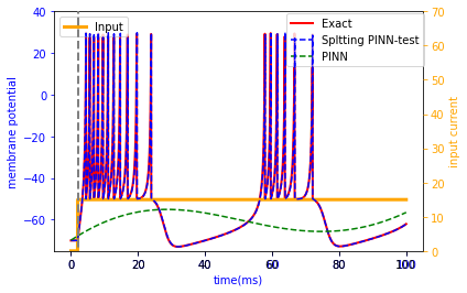
(a)

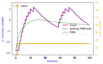
(b)

Figure 3: Izhikevich model: Left: membrane potential versus time. Right: recovery variable versus time.

Table 2: mean relative $L^{2}$ norm of errors for the Izhikevich model.

	training error	testing error
membrane potential	$0.115719\pm 0.008516$	$0.120458\pm 0.008221$
$u$	$0.041201\pm 0.005980$	$0.043186\pm 0.005070$

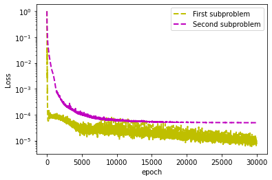
Figure 4: Loss function of the Izhikevich model.

4.3 Hodgkin-Huxley model

Splitting PINN implementation:
For solving the HH model by applying Splitting PINN on interval $[0,T]$, we have used the choice of parameters given in Table 3.

Table 3: Parameter values and their descriptions of the HH neuron model [58].

Parameter	Value	Description
$g_{Na}$	$120\ mS/cm^{2}$	Maximum Na+ current conductance
$g_{K}$	$36\ mS/cm^{2}$	Maximum K+ current conductance
$g_{L}$	$0.3\ mS/cm^{2}$	Maximum leak current conductance
$E_{Na}$	$50\ mV$	Na+ current reversal potential
$E_{K}$	$-77\ mV$	K+ current reversal potential
$E_{L}$	$-54\ mV$	Leak current reversal potential
$C_{m}$	$1\ \mu F\cdot s^{q_{1}-1}/cm^{2}$	Membrane Capacitance
$V_{0}$	$-65$	Initial membrane potential
$m_{0}$	$0.0529$	Initial Na+ current activation
$n_{0}$	$0.3177$	Initial Na+ current inactivation
$h_{0}$	$0.5960$	Initial K+ current activation

Consider $(V^{j},n^{j},m^{j},h^{j})$ to be the solution at $t^{j}=j\Delta t$ with step size $\Delta t$. Then, the following sub-systems on each sub-interval $[t^{j},t^{j+1}]$ are obtained using the Lie splitting method. The first part is,

$$\begin{split}&\frac{dn}{dt}=F_{2}(t,V_{m}^{j},n,m,h),\qquad n(t^{j})=n^{j},\qquad t\in(t^{j},t^{j+1}],\\ &\frac{dm}{dt}=F_{3}(t,V_{m}^{j},n,m,h),\qquad m(t^{j})=m^{j},\qquad t\in(t^{j},t^{j+1}],\\ &\frac{dh}{dt}=F_{4}(t,V_{m}^{j},n,m,h),\qquad h(t^{j})=h^{j}\qquad t\in(t^{j},t^{j+1}].\end{split}$$ (22)

where $V_{m}^{j}$ is the known solution at time $t=t^{j}$. The second part is given by

$$\begin{split}&\frac{dV_{m}}{dt}=F_{1}(t,V_{m},n^{j+1},m^{j+1},h^{j+1}),\qquad V_{m}(t^{j})=V_{m}^{j},\qquad t\in(t^{j},t^{j+1}],\end{split}$$ (23)

and $(n^{j+1},m^{j+1},h^{j+1})$ is the solution obtained from the first part. The splitting approximation of the solution at $t=t^{j+1}$ is $(V_{m}^{j+1},n^{j+1},m^{j+1},h^{j+1})$, and the solution for the whole domain is obtained by repeating this process.

Different kinds of input currents, including step current function and constant current, are considered for solving the HH model.

Step current function: For solving the HH model with the given step current in Figure 5(a) at the time interval $[0,20ms]$, we have used $800$ sub-intervals in the splitting procedure with $40$ training points for solving each sub-problem. The hyperparameters and architecture of PINNs for solving the sub-problems can be found in Table 1.

Constant current: This system is solved at time interval $[0,100ms]$, with $3000$ sub-intervals and $30$ points at each sub-interval. With the given hyperparameters and architectures in Table 1, PINN is used for solving each part, and the solutions are combined to obtain the approximate solutions.

The relative $L^{2}$ norm of errors of approximate solutions are shown in Table 5.

Table 4: mean relative $L^{2}$ norm of errors for HH model with current step function.

	training error	testing error
membrane potential	$0.001155\pm 0.000111$	$0.000886\pm 0.000149$
$n$	$0.002720\pm 5.3\times 10^{-5}$	$0.002712\pm 5.3\times 10^{-5}$
$m$	$0.014316\pm 0.000447$	$0.014071\pm 0.000451$
$h$	$0.002685\pm 7.3\times 10^{-5}$	$0.002680\pm 7.2\times 10^{-5}$,

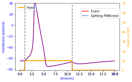
(a)

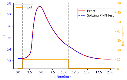
(b)

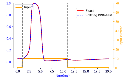
(c)

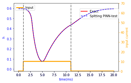
(d)

Figure 5: HH model: comparison of splitting PINN results with the reference solution. (a) membrane potential; (b) activation variable of potassium channel; (c) activation variable of the sodium channel; (d) deactivation variable of the sodium channel. The inset plot shows the step function input current.

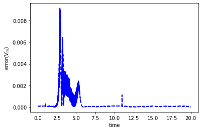
(a)

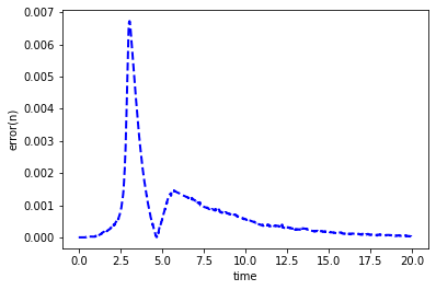
(b)

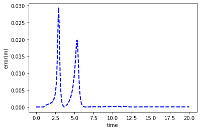
(c)

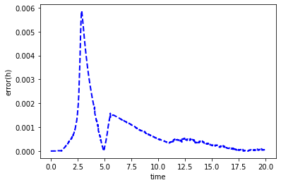
(d)

Figure 6: HH model: absolute error of the normalized solutions using splitting PINN with a current step function. (a) membrane potential; (b) activation variable of potassium channel; (c) activation variable of the sodium channel; (d) deactivation variable of the sodium channel.

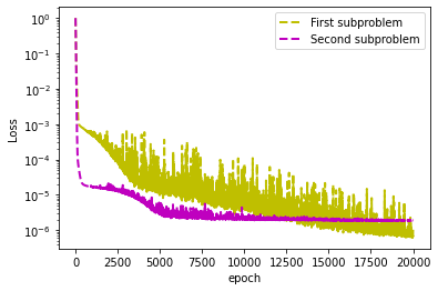
Figure 7: Loss function of the HH model with a current step function.

Table 5: mean relative $L^{2}$ norm of errors for HH model for constant current.

	training error	testing error
membrane potential	$0.009925\pm 0.001957$	$0.009434\pm 0.001877$
$n$	$0.005240\pm 0.000666$	$0.005229\pm 0.000661$
$m$	$0.030731\pm 0.003931$	$0.030364\pm 0.003939$
$h$	$0.007077\pm 0.000899$	$0.007066\pm 0.000898$

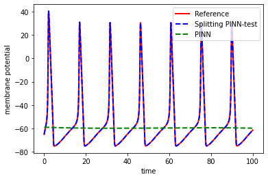
(a)

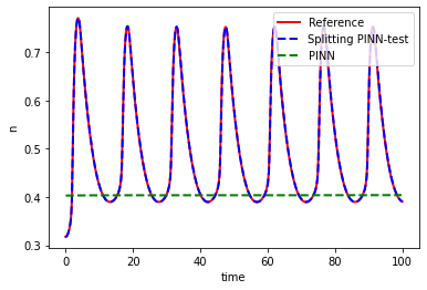
(b)

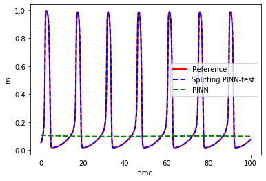
(c)

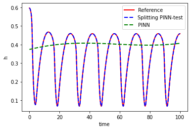
(d)

Figure 8: HH model: comparison of splitting PINN results with the reference solution for constant current input ($I=10\ nA/cm^{2}$). (a) membrane potential; (b) activation variable of potassium channel; (c) activation variable of the sodium channel; (d) deactivation variable of the sodium channel. Note that PINN fails to predict the solution.

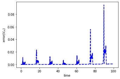
(a)

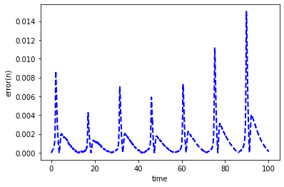
(b)

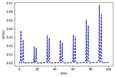
(c)

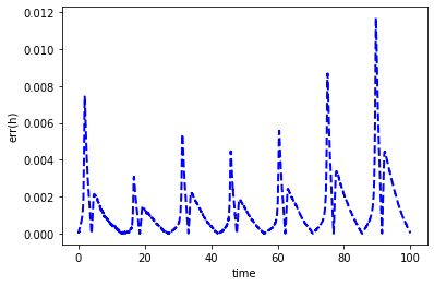
(d)

Figure 9: HH model: absolute error of the normalized solutions using splitting PINN with a constant current ($I=10\ nA/cm^{2}$). (a) membrane potential; (b) activation variable of potassium channel; (c) activation variable of the sodium channel; (d) deactivation variable of the sodium channel.

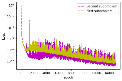
Figure 10: Loss function of the HH model for constant current.

4.4 Fractional Hodgkin-Huxley model

Splitting FPINN implementation:

This problem is solved using the splitting fractional physics-informed neural network (FPINN) approach [48]. In this approach, the memory of the fractional derivative at each sub-interval encompasses the entire domain. So for each sub-interval $[t^{j},t^{j+1}]$ $(0\leq j\leq N_{1}-1)$, by using the developed $L^{1}$ - scheme, we have the following sub-problems:

$$\delta_{t}^{q_{1}}V_{m}^{N_{2}j+l+1}=F_{1}(t^{N_{2}j+l+1},V_{m}^{N_{2}j+l+1},n,m,h),$$ (24)

where

$$\delta_{t}^{q_{1}}V_{m}^{N_{2}j+l+1}=\sum_{k=0}^{N_{2}j+l}b_{k}^{q_{1}}\left[V_{m}(t^{N_{2}j+l+1-k})-V_{m}(t^{N_{2}j+l-k})\right],$$ (25)

and $n$, $m$ and $h$ are the known solutions at $t=t^{N_{2}j+l}$. The second subproblem is

$$\begin{split}\delta_{t}^{q_{2}}n^{N_{2}j+l+1}&=F_{2}(t^{N_{2}j+l+1},V_{m},n^{N_{2}j+l+1},m,h),\\ \delta_{t}^{q_{3}}m^{N_{2}j+l+1}&=F_{3}(t^{N_{2}j+l+1},V_{m},n,m^{N_{2}j+l+1},h),\\ \delta_{t}^{q_{4}}h^{N_{2}j+l+1}&=F_{4}(t^{N_{2}j+l+1},V_{m},n,m,h^{N_{2}j+l+1}).\end{split}$$ (26)

where $V_{m}$ is the solution of the first sub-problem at $t=t^{N_{2}j+l+1}$, $l=0,1,\cdots,N_{2}-1$, and $N_{2}$ is the number of residual points for each sub-interval.

Then, the solutions of sub-systems are combined to obtain the solution of the original system.

This model is solved with the proposed method for $q_{i}=0.8,0.6,0.4$ at time interval $[0,100ms]$, with $2000$ sub-intervals and $40$ residual points in each sub-interval. Each part is solved via FPINN, with the given hyperparameters and network architectures in Table 1.

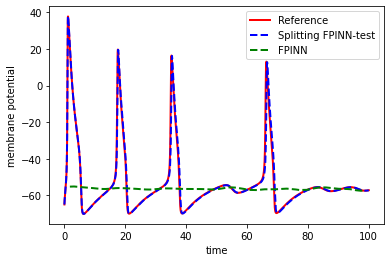
(a)

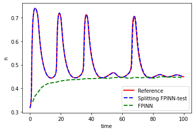
(b)

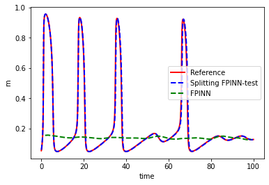
(c)

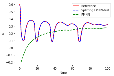
(d)

Figure 11: FO-HH model: comparison of splitting FPINN results with the reference solution for constant current input ($I=20\ nA/cm^{2}$) and fractional order $q_{1}=q_{2}=q_{3}=q_{4}=0.8$. (a) membrane potential; (b) activation variable of potassium channel; (c) activation variable of the sodium channel; (d) deactivation variable of the sodium channel. Note that FPINN fails to predict the solution.

Figure 12: Loss function of the FO-HH model for fractional order $q_{1}=q_{2}=q_{3}=q_{4}=0.8$.

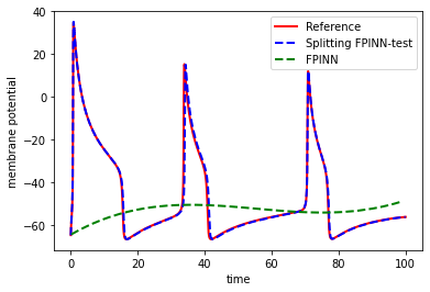
(a)

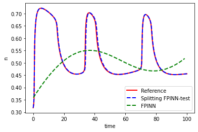
(b)

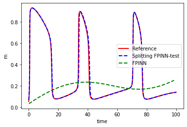
(c)

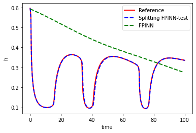
(d)

Figure 13: FO-HH model: comparison of splitting FPINN results with the reference solution for constant current input ($I=20\ nA/cm^{2}$) and fractional order $q_{1}=q_{2}=q_{3}=q_{4}=0.6$. (a) membrane potential; (b) activation variable of potassium channel; (c) activation variable of the sodium channel; (d) deactivation variable of the sodium channel. Note that FPINN fails to predict the solution.

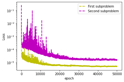
Figure 14: Loss function of the FO-HH model for fractional order $q_{1}=q_{2}=q_{3}=q_{4}=0.6$.

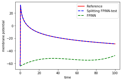
(a)

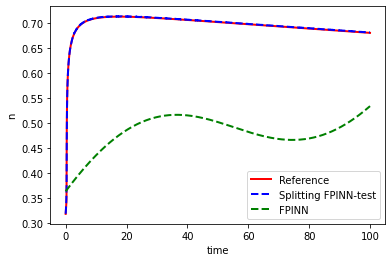
(b)

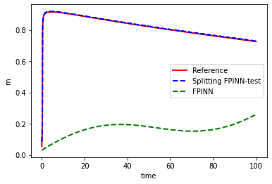
(c)

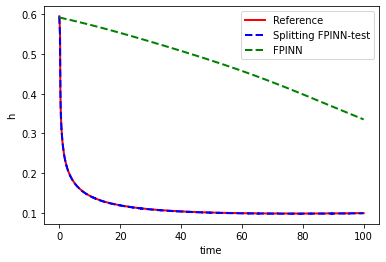
(d)

Figure 15: FO-HH model: comparison of splitting FPINN results with the reference solution for constant current input ($I=20\ nA/cm^{2}$) and fractional order $q_{1}=q_{2}=q_{3}=q_{4}=0.4$. (a) membrane potential; (b) activation variable of potassium channel; (c) activation variable of the sodium channel; (d) deactivation variable of the sodium channel. Note that FPINN fails to predict the solution.

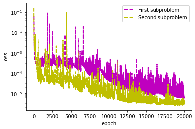
Figure 16: Loss function of the FO-HH model for fractional order $q_{1}=q_{2}=q_{3}=q_{4}=0.4$.

Table 6: mean relative $L^{2}$ norm of errors for FO-HH model for different orders of fractional derivatives. The first and second sub-rows correspond to the training and testing errors, respectively.

	$q_{i}=0.8$	$q_{i}=0.6$	$q_{i}=0.4$
membrane	$0.084252\pm 0.011138$	$0.098086\pm 0.027659$	$0.043236\pm 0.001514$
potential	$0.084460\pm 0.012576$	$0.096949\pm 0.028145$	$0.043241\pm 0.003771$
$n$	$0.024353\pm 0.005469$	$0.023854\pm 0.008417$	$0.001909\pm 8.8\times 10^{-5}$
	$0.024360\pm 0.005527$	$0.023776\pm 0.008435$	$0.001933\pm 0.000177$
$m$	$0.129660\pm 0.035021$	$0.093863\pm 0.031778$	$0.006009\pm 9.4\times 10^{-5}$
	$0.129083\pm 0.035903$	$0.093619\pm 0.032427$	$0.006063\pm 0.000214$
$h$	$0.036292\pm 0.009040$	$0.040947\pm 0.013980$	$0.007536\pm 0.000374$
	$0.036336\pm 0.009121$	$0.040921\pm 0.013963$	$0.007592\pm 0.000649$

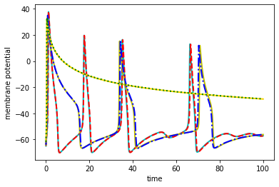
(a)

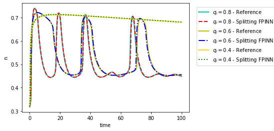
(b)

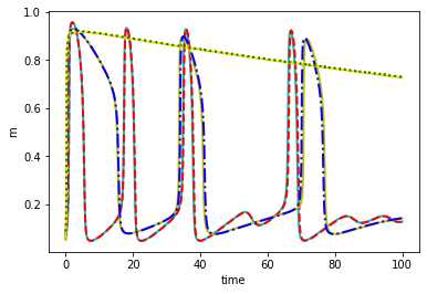
(c)

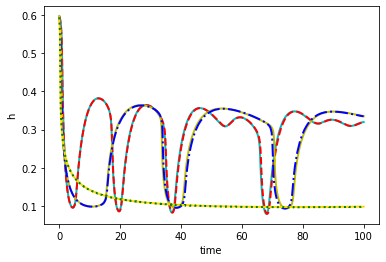
(d)

Figure 17: Plots of the membrane potential and the corresponding activation and deactivation variables of the FO-HH model with constant current $I=20\ nA/cm^{2}$ for different orders of fractional derivatives, obtained using the splitting FPINN.

5 Disccusion

We have presented a deep learning approach for solving nonlinear systems of differential equations. The performance and accuracy of splitting Physics-Informed Neural Networks (PINNs) are studied in the context of solving neuron models. In Section 4.2, the proposed method was used to solve the Izhikevich model. We showed the reference and learned solutions in Figure 3 for equi-distant training and random test datasets. It can be seen that the nonlinear solutions learned by the nonlinear splitting PINN match well with the reference solutions. The relative $L^{2}$ norm of errors for the solutions are presented in Table 2, which shows the method’s capability for this model. The convergence of the loss functions is shown in Figure 4. It can be seen that this function rapidly tends to values lower than $10^{-5}$ and $10^{-4}$ for the first and second sub-problems.

After solving the Izhikevich model, we focus on using the Splitting PINN method for the Hodgkin-Huxley model. In this model, applying input current and changes in voltage resulting from the opening and closing of ion channels lead to the generation of spikes. The amount of input current needed to generate a spike is at least $2.7nA/cm^{2}$, and with increasing input current, the number of spikes increases. In Section 4.3, the voltage is obtained for two states of input current: step function current and constant input current. In the first case, when the current is applied over a given time interval, the voltage increases and produces an action potential (positive peak). After the spike, the potassium channel opens, and the sodium channel closes, causing the voltage to decrease and the neuron to enter a refractory period where the potential is below the resting potential of $V_{rest}=-65mV$. The voltage then slowly returns to $-65mV$. The splitting PINN method was used to calculate approximate solutions and compare them with reference solutions. The results are shown in Figure 5, and the absolute errors are given in Figure 6, which demonstrate the accuracy of the method. The relative $L^{2}$ norm of errors for the current step function is presented in Table 4. The convergence of the loss functions is also shown in Figure 7 and tends to smaller values of $10^{-6}$ and $10^{-5}$ for the first and second sub-problems, respectively.

In the case of a constant input current, the approximate and reference solutions are shown in Figure 8. The proposed method’s effectiveness is demonstrated by comparing the approximate results with the reference and numerical solutions obtained using PINN. The absolute errors of the solutions are shown in Figure 9, and the plots of the loss functions are displayed in Figure 10, which converge to values of $10^{-6}$ for sub-problems. The relative $L^{2}$ norm of errors of the solutions is presented in Table 5. These results demonstrate the capability and accuracy of the proposed algorithm in solving this model.

The fractional-order Hodgkin-Huxley model was also studied in Section 4.4. The system was modeled using Caputo’s fractional derivative and simulated using the proposed method. The effect of memory, associated with fractional order, on firing activity was also examined. To address this, the $L^{1}$ scheme was improved for solving the fractional-order model by proposing using full-domain memory, rather than sub-domain memory, to calculate the fractional derivative. The numerical results obtained using the improved method for $q_{i}=0.8,0.6,0.4$ are shown in Figures 11, 13 and 15, where the approximate results are compared with the reference solutions. The plots of the loss functions are also shown in Figures 12, 14, and 16, demonstrating the efficiency and convergence of the current method. The relative $L^{2}$ norm of errors of the solutions is presented in Table 6, and as shown in the Section, the results are accurate and have converged to the reference solutions.

The voltage responses for the different orders of fractional derivatives under constant input current $I=20$ are also displayed in Figure 17. The Figure demonstrates that various spike patterns can be produced. As $q_{i}$ approaches 1, the firing frequency decreases and results in an increase in the number of spikes in the same time period. Furthermore, the first spike occurs at a later time. Following the cessation of the injected current, the memory-dependent spiking activity can also be observed by applying a step function current. Additionally, the regularity of solutions is observed to depend on the order of fractional derivatives in Figure 17. As $q_{i}$ decreases, the regularity increases. Table 6 shows that, unregular solutions are more sensitive to parameter initialization, leading to a greater standard deviation. To address this issue, the network architecture can be improved.

The results in this section demonstrate high accuracy, and the solutions have converged to the reference values.

6 Conclusion

In this study, we introduced a novel method for solving neuron models represented as systems of differential equations. The Splitting PINN algorithm was demonstrated to be effective and accurate through comparisons with reference solutions and the mean $L^{2}$ relative norm of errors. In addition, the results of the fractional-order Hodgkin-Huxley model highlighted the effect of memory on firing activity and voltage responses, showing that as $q_{i}$ approaches 1, the firing frequency decreases while the number of spikes in the same time period increases.

This research provides valuable insights into the behavior of neuron membranes and the various spike patterns that can be generated. The performance of the proposed method demonstrates its superiority over the vanilla PINN algorithm in solving complex neuron models represented as systems of differential equations. This study contributes to the development of tools for investigating the behavior of neurons and the underlying mechanisms of neural activity.

In conclusion, the proposed Splitting PINN algorithm is a promising method for solving systems of differential equations and provides valuable insights into the behavior of neurons and their underlying mechanisms.

Appendix A PINN implementation for LIF model

In this Section, PINN has been used to solve the LIF model with the given parameters in Table 7. For different input currents in time interval $[0,0.5s]$, the network is trained with $1000$ residual points. Initially, assuming that there is no input current, then if the current $I(t)=0.1A$ is injected into the neuron, the membrane potential tends to $R\cdot I(t)$, which can be seen in Figure 18.

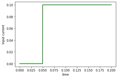
(a) $I(t)$

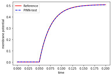
(b) $V(t)$

Figure 18: LIF model: Left: Input current versus time. Right: membrane potential versus time (comparison of PINN results with the reference solutions).

Table 7: Parameter values and their descriptions of LIF model [16, 17].

Parameter	Value	Description
$C_{m}$	$5\times 10^{-3}F$	Membrane Capacity
$R$	$5.1\ \Omega$	Membrane Resistance
$\tau$	$RC_{m}\ s$	Membrane time constant
$V_{rest}$	$0\ V$	Resting membrane potential
$V_{th}$	$1\ V$	Threshold membrane potential

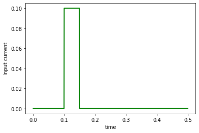
(a) $I_{1}(t)$

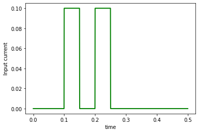
(b) $I_{2}(t)$

(c) $I_{3}(t)$

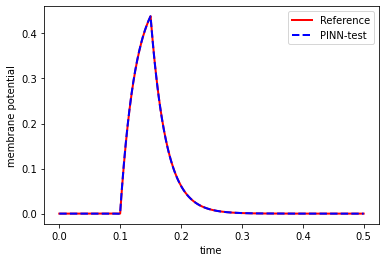
(d) $V_{1}(t)$

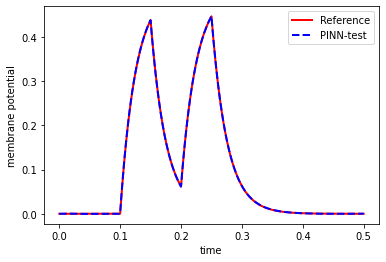
(e) $V_{2}(t)$

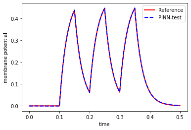
(f) $V_{3}(t)$

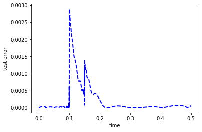
(g) absolute error of $V_{1}(t)$

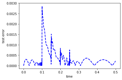
(h) absolute error of $V_{2}(t)$

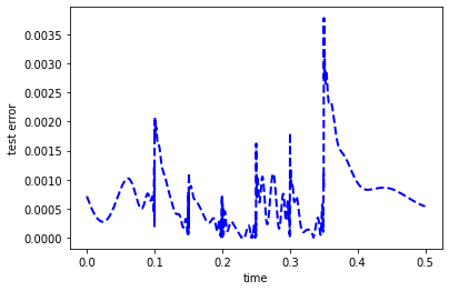
(i) absolute error of $V_{3}(t)$

Figure 19: LIF model; (a)-(c): input step function currents, (d)-(f): comparison of the PINN results with the reference solutions, and (g)-(i): the error results of PINN.

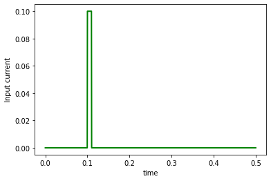
(a) $I_{1}(t)$

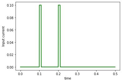
(b) $I_{2}(t)$

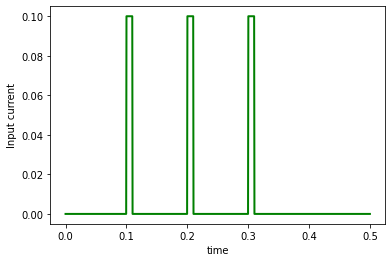
(c) $I_{3}(t)$

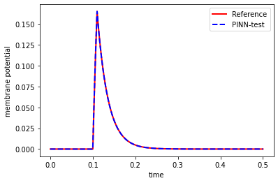
(d) $V_{1}(t)$

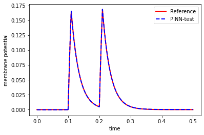
(e) $V_{2}(t)$

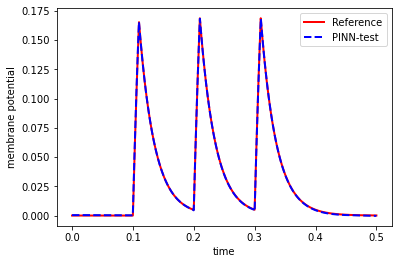
(f) $V_{3}(t)$

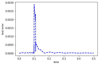
(g) absolute error of $V_{1}(t)$

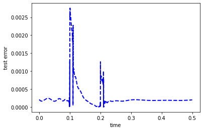
(h) absolute error of $V_{2}(t)$

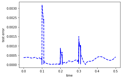
(i) absolute error of $V_{3}(t)$

Figure 20: LIF model; (a)-(c): input spikes, (d)-(f): comparison of the PINN results with the reference solutions, and (g)-(i): the error results of PINN.

The membrane potentials for different forms of step current function have been displayed in Figures 19–21. By applying an input current in a time step, the membrane potential increases, and then after cutting off the input current, the potential decreases with the time constant $\tau$.

If the width of the injected current increases, the membrane potential increases at a slower rate. As the input current pulse amplitude decreases, the membrane potential jumps directly up in a short time. The membrane potential decreases over time in the absence of an input current.

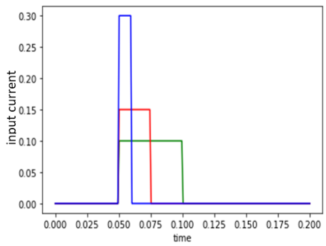
(a) different input currents

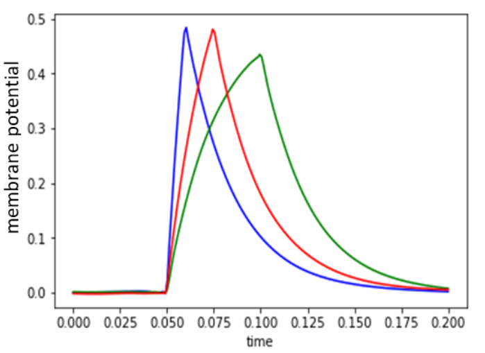
(b) membrane potentials

Figure 21: LIF model: (a) Input currents with different lengths and heights, (b) corresponding membrane potentials by using PINN

So far, we have seen the neuron’s behavior against different input currents (spikes). We need to apply a voltage threshold condition to the model to see the process of generating output spikes by a neuron. According to this condition, if the membrane potential exceeds this threshold, the neuron produces a spike, and after firing the spike, the membrane potential returns to its initial state (resting state).

If the injected current increases, the membrane potential approaches the threshold faster, and the firing rate increases. Similar behavior in firing frequency can be produced by lowering the threshold. These experiments hold for the constant current application, but neurons may be more likely to receive spikes in other cases.

The approximate solutions of this model, when the threshold voltage is applied, have been shown in Figure 22. In this case, for solving the problem in $[0,0.2s]$, we have used $1000$ sub-intervals and $20$ points in each sub-interval. Furthermore, for solving the problem in each sub-interval, PINN has been used with the given architecture in Table 1.

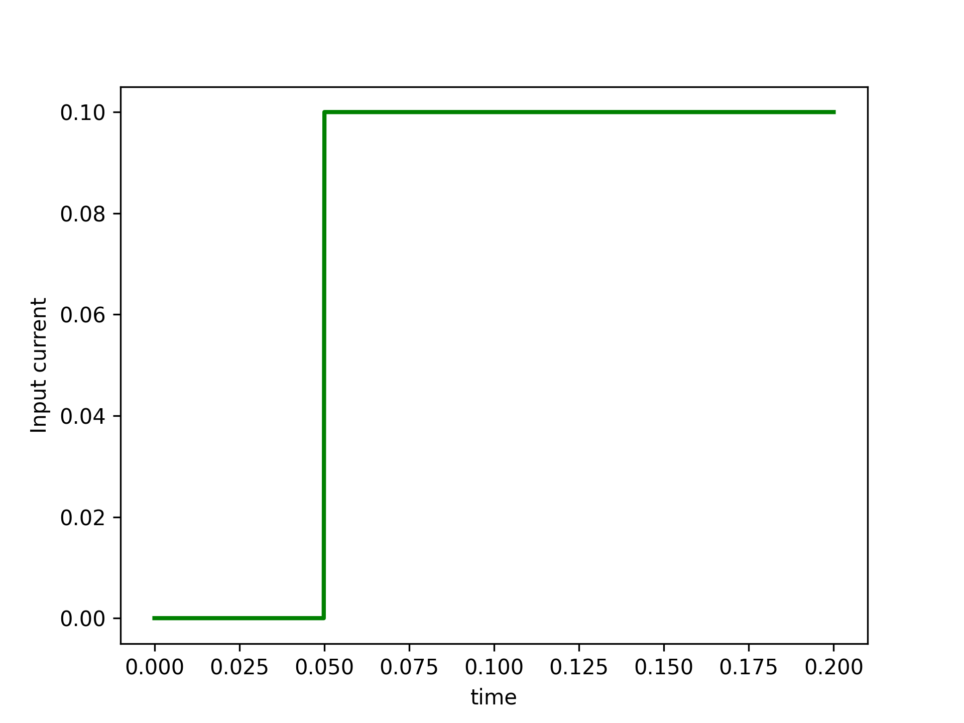
(a) input current $I_{1}(t)$

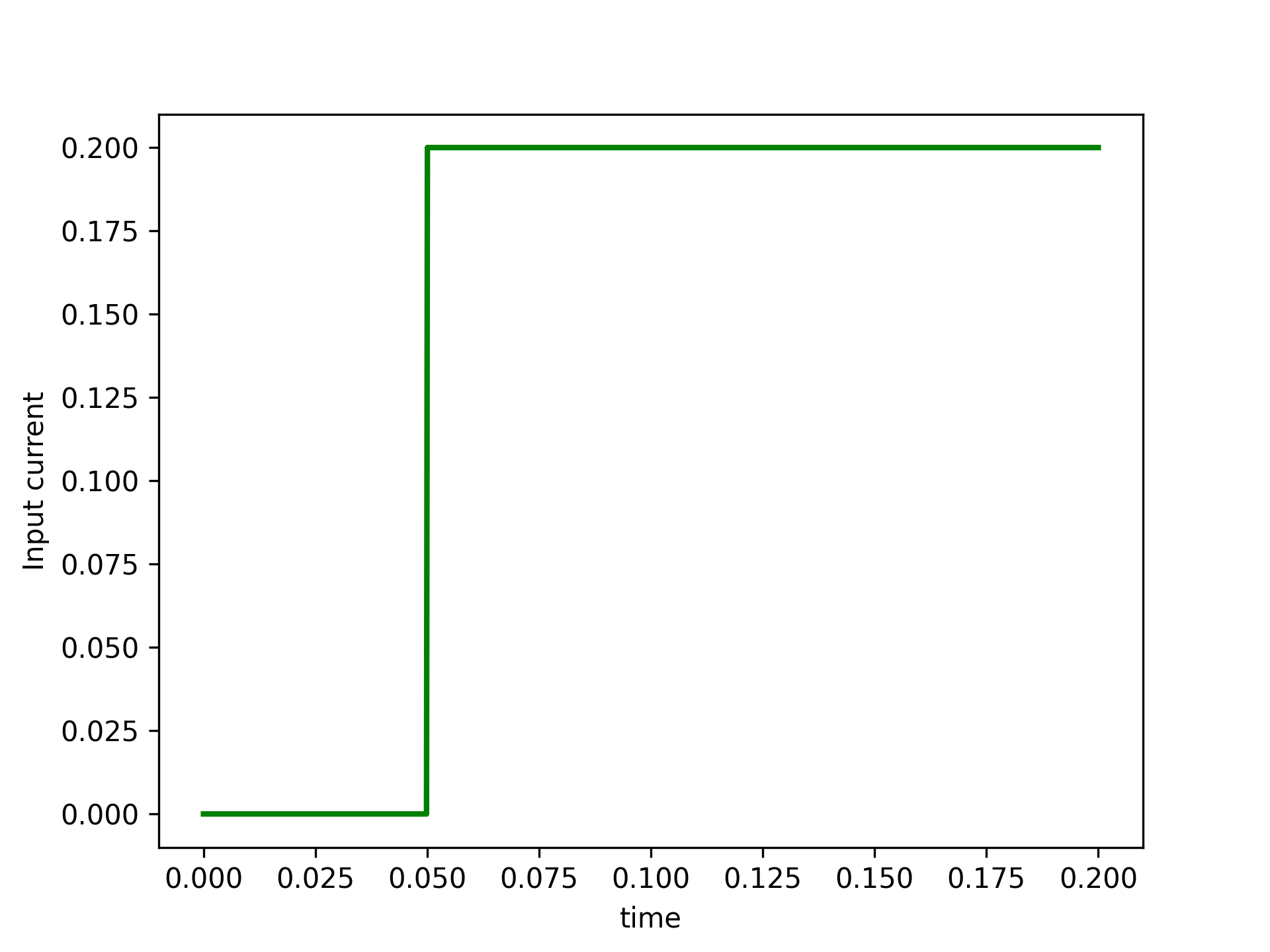
(b) input current $I_{2}(t)$

(c) input current $I_{3}(t)$

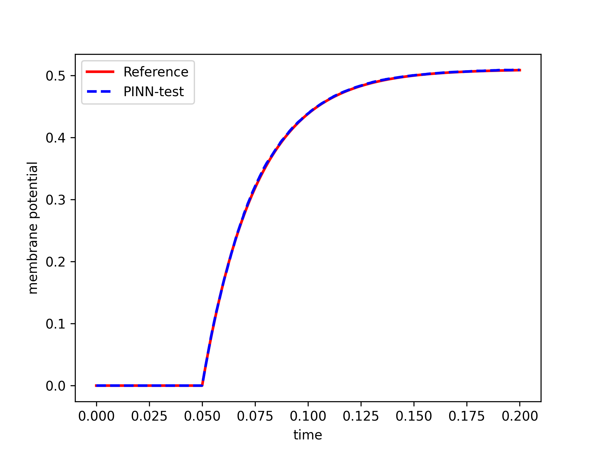
(d) voltage response $V_{1}$

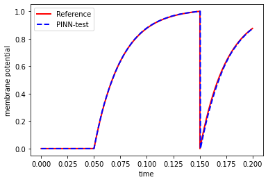
(e) voltage response $V_{2}$

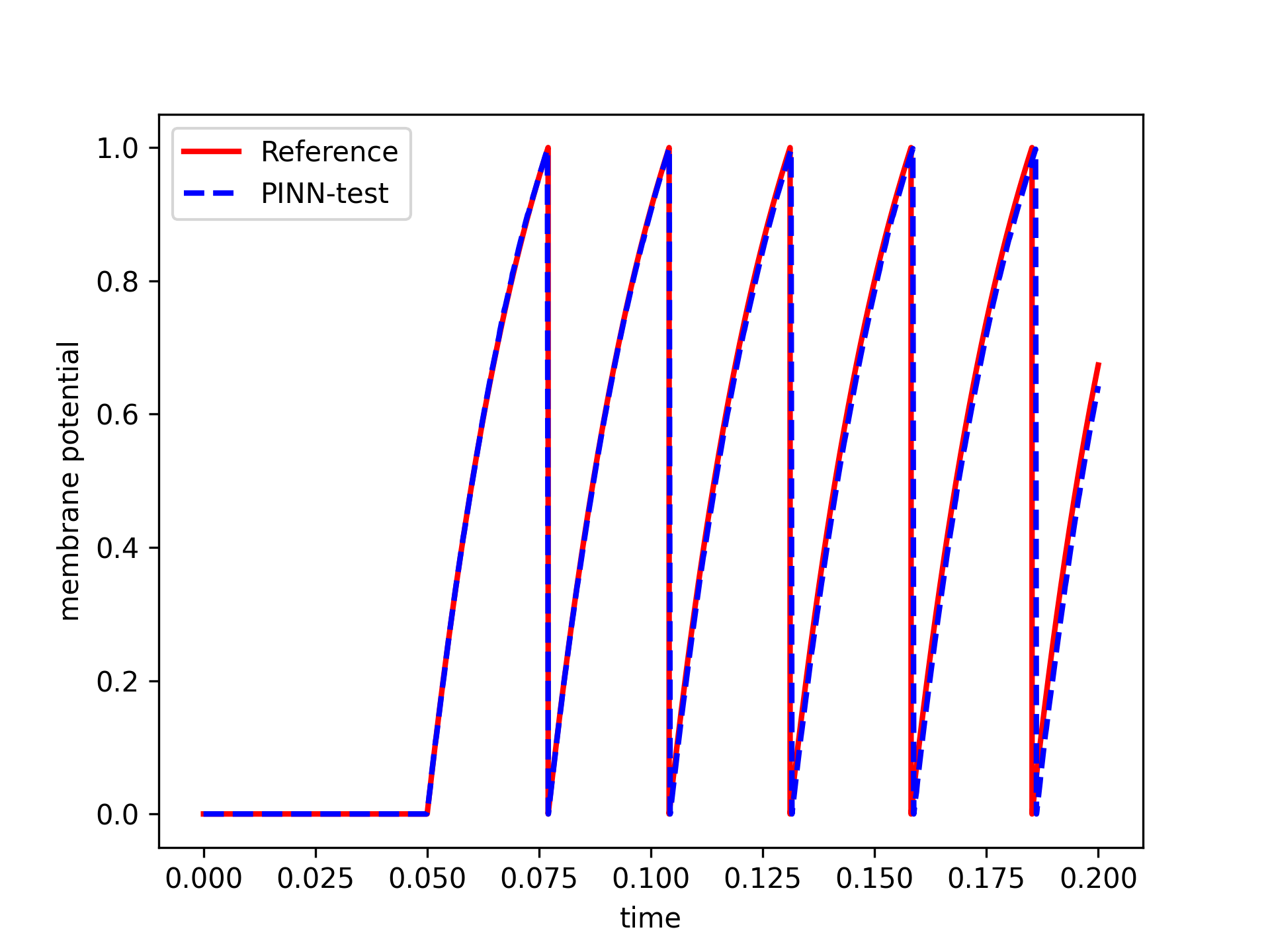
(f) voltage response $V_{3}$

(g) no output

(h) output of neuron

(i) output of neuron

Figure 22: LIF model; (a)-(c): input currents, (d)-(f): comparison of the PINN results with the reference solutions, and (g)-(i): output spikes.

Appendix B Reference solutions

We present a highly efficient and accurate spectral collocation method for obtaining the reference solutions of the fractional differential equations studied in the paper. Consider the following system of FODEs

$${}_{C}D_{0,t}^{\alpha_{k}}U_{k}(t)=f_{k}(t,U),\quad 0<t\leq T,\quad k=1,2...,d,d\in\mathbb{N},$$ (27)

subject to the initial condition $U_{k}(0)=\phi_{k},f_{k}(t,U),U=(U_{1},U_{2},...,U_{d})$.

We apply the fast time-stepping spectral collocation method to solve (27). Divide the interval into subintervals $[t^{k-1},t^{k}]$ such that $[0,T]=[t^{0},t^{1}]\cup[t^{1},t^{2}]\cup\cdot\cup[t^{N-1},t^{N}]$ and $t^{N}=T$, $N$ is a positive number. Let $p$ be a positive number and $\{x_{j}\}_{j=0}^{p}$ be the Legendre–Gauss–Lobatto (LGL) quadrature points on the standard interval $[-1,1]$. Then, the LGL quadrature points $\{t^{k}_{j}\}_{j=0}^{p}$ in the interval $[t^{k-1},t^{k}]$ can be written as

$$t_{j}^{k}=\frac{1}{2}\left[(t^{k}-t^{k-1})x_{j}+t^{k-1}+t^{k}\right].$$

Denote $\Pi^{p}$ the interpolation operator as

$$\Pi^{p}u(t)|_{t\in[t^{k-1},t^{k}]}=\sum_{j=0}^{p}u(t^{k}_{j})\ell^{k}_{j}(t),\qquad\ell^{k}_{j}(t)=\prod_{q=0,q\neq j}^{p}\frac{t-t^{k}_{q}}{t^{k}_{j}-t^{k}_{q}}.$$

Next, we show the fast calculation of ${}_{C}D_{0,t}^{\alpha}u(t)$, the algorithm is illustrated by the following Step 1)–Step 4).

• Step 1) Find a sum-of-exponentials to approximate the kernel function $k_{-\alpha}(t)$ as

  $$k_{-\alpha}(t)=\frac{t^{-\alpha-1}}{\Gamma(-\alpha)}=\sum_{j=1}^{Q}w_{j}e^{-\lambda_{j}t}+O(\varepsilon t^{-\alpha-1}),\quad t\in[t_{1},T],$$ (28)

  where $\varepsilon$ is the relative error, $Q>1$ is a positive integer, and

  $$\lambda_{j}=e^{y_{j}},\quad w_{j}=-\frac{\sin(\alpha\pi)}{\pi}\Delta ye^{(1+\alpha)y_{j}}.$$

  Here, $y_{j}=y_{\min}+j\Delta y$, $\Delta y=(y_{\max}-y_{\min})/(Q-1)$, and

  $$y_{\min}=(1+\alpha)^{-1}\ln(\varepsilon_{0})-\ln(T),\quad\varepsilon_{0}=10^{-16},$$

  $$y_{\max}=\log\left(\frac{-\ln(\varepsilon_{0})+(1+\alpha)\ln(t_{1})}{0.5t_{1}}\right),\quad\varepsilon_{0}=10^{-16}.$$

• Step 2) For $t>t^{n-1}$, divide

  $${}_{C}D_{0,t}^{\alpha}u(t)=P.V.\int_{0}^{t}k_{-\alpha}(t-s)(u(s)-u(0))\ dx[s]$$

  into two parts as

  $${}_{C}D_{0,t}^{\alpha}u(t)=\underbrace{P.V.\int_{t^{n-1}}^{t}k_{-\alpha}(t-s)u(s)\ dx[s]-\frac{t^{-\alpha}u(0)}{\Gamma(1-\alpha)}}_{L^{\alpha}u}+\underbrace{\int_{0}^{t^{n-1}}k_{-\alpha}(t-s)u(s)\ dx[s]}_{H^{\alpha}u},$$

  where $P.V.$ stands for the principal value with

  $$P.V.\int_{a}^{t}k_{-\alpha}(t-s)u(s)\ dx[s]=\frac{1}{\Gamma(1-\alpha)}\frac{\ dx[]}{\ dx[t]}\int_{a}^{t}(t-s)^{-\alpha}u(s)\ dx[s].$$

  For $j=1,2,...,N$, the local part $Lu(t_{j}^{n})$ is calculated by

  $$L^{\alpha}u(t_{j}^{n})\approx L^{\alpha}u_{j}^{n}=P.V.\int_{t^{n-1}}^{t_{j}^{n}}k_{-\alpha}(t_{j}^{n}-s)(\Pi^{p}u)(s)\ dx[s]-\frac{u(0)}{\Gamma(1-\alpha)}(t_{j}^{n})^{-\alpha}.$$

• Step 3) By (28), the history part $H^{\alpha}u(t_{j}^{n}),j=1,2,...,p$, is approximated by

  $$H^{\alpha}u(t_{j}^{n})\approx \int_{0}^{t^{n-1}}k_{-\alpha}(t_{j}^{n}-s)\Pi^{p}u(s)\ dx[s]$$ (29)

  $$\approx \sum_{k=1}^{Q}w_{k}\int_{0}^{t^{n-1}}e^{-\lambda_{k}(t_{j}^{n}-s)}\Pi^{p}u(s)\ dx[s]$$

  $$= \sum_{k=1}^{Q}w_{k}e^{-\lambda_{k}(t_{j}^{n}-t^{n-1})}\underbrace{\int_{0}^{t^{n-1}}e^{-\lambda_{k}(t^{n-1}-s)}\Pi^{p}u(s)\ dx[s]}_{Y_{k}(t^{n-1})}$$

  $$= \sum_{k=1}^{Q}w_{k}e^{-\lambda_{k}(t_{j}^{n}-t^{n-1})}Y_{k}(t^{n-1})={}_{F}H^{\alpha}u_{j}^{n},$$

  where $Y_{k}(t)$ satisfies the following linear ODE

  $$Y_{k}^{\prime}(t)=-\lambda_{k}Y_{k}(t)+\Pi^{p}u(t),\qquad Y_{k}(0)=0,$$

  which can be exactly solved by the following recurrence formula

  $$Y_{k}(t^{n-1})=e^{-\lambda_{k}(t^{n-1}-t^{n-2})}Y_{j}(t^{n-2})+\int_{t^{n-2}}^{t^{n-1}}e^{-\lambda_{k}(t^{n-1}-t)}\Pi^{p}u(t)\ dx[t],\quad Y_{j}(0)=0.$$

• Step 4) Output ${}_{F}\delta_{t}^{\alpha}u^{n}_{j}=L^{\alpha}u^{n}_{j}+{}_{F}H^{\alpha}u^{n}_{j}$, $j=1,2,...,p$.

We are now in a position to develop the fast time-stepping collocation method for solving (27).

The fast time-stepping collocation method for (27) is: Given $U_{\ell,j}^{k},k\leq n-1,0\leq j\leq p,n\geq 1$, find $U^{n}_{\ell,j}$, such that

$${}_{F}\delta_{t}^{\alpha}U^{n}_{j}=f(t^{n}_{j},U^{n}_{\ell,j}),\qquad 1\leq j\leq p,\quad 1\leq\ell\leq d.$$ (30)

The above equation can be rewritten as

$$P.V.\int_{t^{n-1}}^{t_{j}^{n}}k_{-\alpha_{\ell}}(t_{j}^{n}-s)(\Pi^{p}U_{\ell})(s)\ dx[s]-f_{\ell}(t^{n},U^{n}_{\ell,j})$$ (31)

$$= -{}_{F}H^{\alpha_{\ell}}U^{n}_{\ell,j}+\frac{(t_{j}^{n})^{-\alpha_{\ell}}}{\Gamma(1-\alpha_{\ell})}\phi_{\ell},\quad 1\leq j\leq N,1\leq\ell\leq d.$$

The unknowns $u_{j}^{n}(1\leq j\leq N)$ in the above nonlinear system can be derived by the Newton iteration method.

We can rewrite the FOHH model (22)–(23) can be solved by (31).

Some computational issues are addressed below.

• Generally speaking, the solution of the FODE, e.g., (27), has a singularity at the origin ($t=0$ for (27)), we need to refine the mesh near the origin such that high accurate numerical solutions are obtained. For the numerical method (31), for $t\in[0,\Delta T]$, the mesh $t^{n}$ can be defined by $t^{n}=\Delta T(n/M_{1})^{r}$, $r\geq 1$. For $t\in[\Delta T,T]$, the uniform mesh is used which can be given by $t^{n}=t^{M_{1}}+(n-M_{1})\Delta t$, $\Delta t=(T-\Delta T)/M_{2}$, $M_{2}=\lfloor(T-\Delta T)/(t^{M_{1}}-t^{M_{1}-1})\rfloor$.

• For the fractional LIF model with the current $I$ being piecewise constant, the solution also has a singularity at the points of the discontinuity of $I(t)$. We can use the strategy of (i) to refine the mesh near the discontinuity points when we use the method (31) to solve the fractional LIF.

References

- [1] S. A. Aamir, Y. Stradmann, P. Müller, C. Pehle, A. Hartel, A. Grübl, J. Schemmel, and K. Meier, An accelerated LIF neuronal network array for a large-scale mixed-signal neuromorphic architecture, IEEE Transactions on Circuits and Systems I: Regular Papers 65 (2018), no. 12, 4299–4312.
- [2] A. M. AbdelAty, M. E. Fouda, and A. M. Eltawil, On numerical approximations of fractional-order spiking neuron models, Communications in Nonlinear Science and Numerical Simulation 105 (2022), 106078.
- [3] M. Armanyos and A. G. Radwan, Fractional-order Fitzhugh-Nagumo and Izhikevich neuron models, 2016 13th International Conference on Electrical Engineering/Electronics, Computer, Telecommunications and Information Technology (ECTI-CON), 2016, pp. 1–5.
- [4] G. Ascione and E. Pirozzi, On fractional stochastic modeling of neuronal activity including memory effects, Computer Aided Systems Theory – EUROCAST 2017 (Cham) (R. Moreno-Díaz, F. Pichler, and A. Quesada-Arencibia, eds.), Springer International Publishing, 2018, 3–11.
- [5] A. Baydin, B. A. Pearlmutter, A. A. Radul, and J. M. Siskind, Automatic differentiation in machine learning: A survey, Journal of Machine Learning Research 18 (2017), no. 1, 5595–5637.
- [6] C. Beck, S. Becker, P. Cheridito, A. Jentzen, and A. Neufeld, Deep splitting method for parabolic PDEs, SIAM Journal on Scientific Computing 43 (2021), no. 5, A3135–A3154.
- [7] B. Benjamin, P. Gao, E. McQuinn, S. Choudhary, A. Chandrasekaran, J. M. Bussat, R. Alvarez-Icaza, J. Arthur, P. Merolla, and K. Boahen, Neurogrid: A mixed-analog-digital multichip system for large-scale neural simulations, Proceedings of the IEEE 102 (2014), 1–18.
- [8] A. Borst and F. E. Theunissen, Information theory and neural coding, Nature neuroscience 2 (1999), no. 11, 947—957.
- [9] O. Brandibur and E. Kaslik, Stability analysis for a fractional-order coupled Fitzhugh-Nagumo-type neuronal model, Fractal and Fractional 6 (2022), no. 5, 257.
- [10] R. Brette, M. Lilith, T. Carnevale, M. Hines, D. Beeman, J. Bower, M. Diesmann, A. Morrison, P. Goodman, F. Harris, M. Zirpe, T. Natschläger, D. Pecevski, B. Ermentrout, M. Djurfeldt, A. Lansner, O. Rochel, T. Viéville, E. Muller, and A. Destexhe, Simulation of networks of spiking neurons: A review of tools and strategies, Journal of computational neuroscience 23 (2008), 349–398.
- [11] C. Chen, Z. Wang, and Y. Yang, A new operator splitting method for american options under fractional Black-Scholes models, Computers and Mathematics with Applications 77 (2019), no. 8, 2130–2144.
- [12] J. M. Chignon, J. P. Lepine, and J. Ades, Panic disorder in cardiac outpatients, American Journal of Psychiatry 150 (1993), no. 5, 780–785.
- [13] A. Dokoumetzidis and P. Macheras, Fractional kinetics in drug absorption and disposition processes, Journal of pharmacokinetics and pharmacodynamics 36 (2009), no. 2, 165—178.
- [14] A. Dokoumetzidis, R. Magin, and P. Macheras, Fractional kinetics in multi-compartmental systems, Journal of pharmacokinetics and pharmacodynamics 37 (2010), 507–24.
- [15] . Einkemmer and A. Ostermann, Overcoming order reduction in diffusion-reaction splitting. part 1: Dirichlet boundary conditions, SIAM Journal on Scientific Computing 37 (2015), no. 3, A1577–A1592.
- [16] J. K. Eshraghian, snntorch. online: https://github.com/jeshraghian/snntorch, 2021.
- [17] J. K. Eshraghian, M. Ward, E. Neftci, X. Wang, G. Lenz, G. Dwivedi, M. Bennamoun, D. S. Jeong, and W. D. Lu, Training spiking neural networks using lessons from deep learning, arXiv preprint: 2109.12894, 2021.
- [18] E. Faou, A. Ostermann, and K. Schratz, Analysis of exponential splitting methods for inhomogeneous parabolic equations, IMA Journal of Numerical Analysis 35 (2014), no. 1, 161–178.
- [19] A. Ganguly, M. Saha, A. Ghosh, U. Maity, J. P. Kucera, and S. Raha, The method of hybrid functions for the numerical solution of the Hodgkin-Huxley model, IFAC-PapersOnLine 55 (2022), no. 1, 623–630, 7th International Conference on Advances in Control and Optimization of Dynamical Systems ACODS 2022.
- [20] W. Gerstner and W. M. Kistler, Spiking neuron models: Single neurons, populations, plasticity, Cambridge University Press, 2002.
- [21] W. Gerstner, W. M. Kistler, R. Naud, and L. Paninski, Neuronal dynamics: From single neurons to networks and models of cognition, Cambridge University Press, 2014.
- [22] A. H. Glassman and J. T. Bigger Jr, Cardiovascular Effects of Therapeutic Doses of Tricyclic Antidepressants: A Review, Archives of General Psychiatry 38 (1981), no. 7, 815–820.
- [23] E. Haghighat, D. Amini, and R. Juanes, Physics-informed neural network simulation of multiphase poroelasticity using stress-split sequential training, Computer Methods in Applied Mechanics and Engineering 397 (2022), 115–141.
- [24] A. L. Hodgkin and A. F. Huxley, A quantitative description of membrane current and its application to conduction and excitation in nerve, The Journal of Physiology 117 (1952), no. 4, 500–544.
- [25] H. Holden, K. H. Karlsen, and K. A. Lie, Splitting methods for partial differential equations with rough solutions: Analysis and matlab programs, vol. 11, European Mathematical Society, 2010.
- [26] E. M. Izhikevich, Simple model of spiking neurons, IEEE Transactions on Neural Networks 14 (2003), no. 6, 1569–1572.
- [27] E. M. Izhikevich, Which model to use for cortical spiking neurons?, Neural Networks, IEEE Transactions on 15 (2004), 1063 – 1070.
- [28] A. D. Jagtap, K. Kawaguchi, and G. Karniadakis, Adaptive activation functions accelerate convergence in deep and physics-informed neural networks, Journal of Computational Physics 404 (2020), 109136.
- [29] A. D. Jagtap, E. Kharazmi, and G. Karniadakis, Conservative physics-informed neural networks on discrete domains for conservation laws: Applications to forward and inverse problems, Computer Methods in Applied Mechanics and Engineering 365 (2020), 113028.
- [30] E. Kharazmi, Z. Zhang, and G. Karniadakis, hp-VPINNs: Variational physics-informed neural networks with domain decomposition, Computer Methods in Applied Mechanics and Engineering 374 (2021), 113547.
- [31] M. M. A. Khater, R. A. M. Attia, A. H. Abdel‐Aty, S. A. Khalek, Y. Al‐Hadeethi, and D. Lu, On the computational and numerical solutions of the transmission of nerve impulses of an excitable system (the neuron system), Journal of Intelligent and Fuzzy Systems 38 (2020), 2603–2610.
- [32] C. Koch and I. Segev, Methods in neuronal modeling: From ions to networks, second ed., MIT Press, Cambridge, MA, USA, 1998.
- [33] C. Li and F. Zeng, Finite difference methods for fractional differential equations, International Journal of Bifurcation and Chaos 22 (2012), no. 04, 1230014.
- [34] D. Li, C. Quan, and J. Xu, Stability and convergence of Strang splitting. part i: Scalar Allen-Cahn equation, Journal of Computational Physics 458 (2022), 111087.
- [35] Y. Lin and C. Xu, Finite difference/spectral approximations for the time-fractional diffusion equation, Journal of Computational Physics 225 (2007), no. 2, 1533–1552.
- [36] D. Liu and Y. Wang, A dual-dimer method for training physics-constrained neural networks with minimax architecture, Neural Networks 136 (2021), 112–125.
- [37] L Long and G. Fang, A review of biologically plausible neuron models for spiking neural networks, AIAA Infotech at Aerospace 2010, AIAA Infotech at Aerospace 2010, American Institute of Aeronautics and Astronautics Inc., 2010.
- [38] L. Lu, X. Meng, S. Cai, Z. Mao, S. Goswami, Z. Zhang, and G. Karniadakis, A comprehensive and fair comparison of two neural operators (with practical extensions) based on fair data, Computer Methods in Applied Mechanics and Engineering 393 (2022), 114778.
- [39] W. Maass, Networks of spiking neurons: The third generation of neural network models, Neural Networks 10 (1997), no. 9, 1659–1671.
- [40] R. L. Magin, Fractional calculus models of complex dynamics in biological tissues, Computers and Mathematics with Applications 59 (2010), no. 5, 1586–1593.
- [41] R. L. Magin and M. Ovadia, Modeling the cardiac tissue electrode interface using fractional calculus, Journal of Vibration and Control 14 (2008), no. 9-10, 1431–1442.
- [42] L. D. McClenny and U. M. Braga-Neto, Self-adaptive physics-informed neural networks using a soft attention mechanism, arXiv preprint: 2009.04544, 2020.
- [43] R. I. McLachlan, G. Quispel, , and W. Reinout, Splitting methods, Acta Numerica 11 (2002), 341–434.
- [44] Xuhui Meng and George Em Karniadakis, A composite neural network that learns from multi-fidelity data: Application to function approximation and inverse pde problems, Journal of Computational Physics 401 (2020), 109020.
- [45] P. A. Merolla, J. V. Arthur, R. Alvarez-Icaza, A. S. Cassidy, J. Sawada, F. Akopyan, B. L. Jackson, N. Imam, C. Guo, Y. Nakamura, B. Brezzo, I. Vo, S. K. Esser, R. Appuswamy, B. Taba, A. Amir, M. D. Flickner, W. P. Risk, R. Manohar, and D. S. Modha, Artificial brains. a million spiking-neuron integrated circuit with a scalable communication network and interface, Science (New York, N.Y.) 345 (2014), no. 6197, 668—673.
- [46] A. Mondal, S. K. Sharma, R. K. Upadhyay, and A. Mondal, Firing activities of a fractional-order Fitzhugh-Rinzel bursting neuron model and its coupled dynamics, Scientific Reports 9 (2019), 15721.
- [47] K. B. Oldham and J. Spanier (eds.), The fractional calculus: Theory and applications of differentiation and integration to arbitrary order, Mathematics in Science and Engineering, vol. 111, Elsevier, 1974.
- [48] G. Pang, L. Lu, and G. Karniadakis, FPINNs: Fractional physics-informed neural networks, SIAM Journal on Scientific Computing 41 (2019), no. 4, A2603–A2626.
- [49] I. Petráš and R. L. Magin, Simulation of drug uptake in a two compartmental fractional model for a biological system., Communications in nonlinear science & numerical simulation 16 12 (2011), 4588–4595.
- [50] M. Raissi, P. Perdikaris, and G. Karniadakis, Multistep neural networks for data-driven discovery of nonlinear dynamical systems, arXiv preprint: 1801.01236, 2018.
- [51] S. Shekarpaz and H. Azari, An inverse problem of identifying two unknown parameters in parabolic differential equations, Iranian Journal of Science and Technology, Transactions A: Science 42 (2018), 2045–2052.
- [52] S. Shekarpaz and H. Azari, Splitting method for an inverse source problem in parabolic differential equations: Error analysis and applications, Numerical Methods for Partial Differential Equations 36 (2020), no. 3, 654–679.
- [53] S. Shekarpaz, M. Azizmalayeri, and M. H. Rohban, Piat: Physics informed adversarial training for solving partial differential equations, arXiv preprint: 2207.06647, 2022.
- [54] H. H. Sherief, A. M. A. El-Sayed, S. H. Behiry, and W. E. Raslan, Using fractional derivatives to generalize the hodgkin–huxley model, Fractional Dynamics and Control (D. Baleanu, J. A. T. Machado, and A. C. J. Luo, eds.), Springer New York, New York, NY, 2012, pp. 275–282.
- [55] K. Shukla, A. D. Jagtap, and G. Karniadakis, Parallel physics-informed neural networks via domain decomposition, arXiv preprint: 2104.10013, 2021.
- [56] G. Strang, On the construction and comparison of difference schemes, SIAM Journal on Numerical Analysis 5 (1968), 506–517.
- [57] W. Tan, C. Fu, C. Fu, W. Xie, and H. Cheng, An anomalous subdiffusion model for calcium spark in cardiac myocytes, Applied Physics Letters 91 (2007), no. 18, 183901.
- [58] W. Teka, D. Stockton, and F. Santamaria, Power-law dynamics of membrane conductances increase spiking diversity in a Hodgkin-Huxley model, PLOS Computational Biology 12 (2016), no. 3, 1–23.
- [59] W. W. Teka, R. K. Upadhyay, and A. Mondal, Fractional-order leaky integrate-and-fire model with long-term memory and power law dynamics, Neural Networks 93 (2017), 110–125.
- [60] W. W. Teka, R. K. Upadhyay, and A. Mondal, Spiking and bursting patterns of fractional-order Izhikevich model, Communications in Nonlinear Science and Numerical Simulation 56 (2018), 161–176.
- [61] M. F. Tolba, A. H. Elsafty, M. Armanyos, L. A. Said, A. H. Madian, and A. G. Radwan, Synchronization and FPGA realization of fractional-order Izhikevich neuron model, Microelectronics Journal 89 (2019), 56–69.
- [62] H. F. Trotter, On the product of semi-groups of operators, Proceedings of the American Mathematical Society 10 (1959), no. 4, 545–551.
- [63] S. H. Weinberg, Membrane capacitive memory alters spiking in neurons described by the fractional-order Hodgkin-Huxley model, PLOS ONE 10 (2015), no. 5, 1–27.
- [64] S. H. Weinberg, Membrane capacitive memory alters spiking in neurons described by the fractional-order Hodgkin-Huxley model, PLOS ONE 10 (2015), no. 5, 1–27.
- [65] S. Westerlund and L. Ekstam, Capacitor theory, IEEE Transactions on Dielectrics and Electrical Insulation 1 (1994), no. 5, 826–839.
- [66] L. Yang, X. Meng, and G. Karniadakis, B-PINNs: Bayesian physics-informed neural networks for forward and inverse pde problems with noisy data, Journal of Computational Physics 425 (2021), 109913.
- [67] M. W. Yasin, M. S. Iqbal, N. Ahmed, A. Akgül, A. Raza, M. Rafiq, and M. B. Riaz, Numerical scheme and stability analysis of stochastic Fitzhugh-Nagumo model, Results in Physics 32 (2022), 105023.
- [68] D. Zhang, L. Guo, and G. Karniadakis, Learning in modal space: Solving time-dependent stochastic pdes using physics-informed neural networks, SIAM Journal on Scientific Computing 42 (2020), no. 2, A639–A665.
- [69] Y. Zhu, N. Zabaras, P. S. Koutsourelakis, and P. Perdikaris, Physics-constrained deep learning for high-dimensional surrogate modeling and uncertainty quantification without labeled data, Journal of Computational Physics 394 (2019), 56–81.