Thermal and optical conductivity in the Holstein model at half filling and at finite temperature in the Luttinger-liquid and charge-density-wave regime

Abstract

Electron-phonon interactions play a key role in many branches of solid-state physics. Here, our focus is on the transport properties of one-dimensional systems, and we apply efficient real-time matrix-product state methods to compute the optical and thermal conductivities of Holstein chains at finite temperatures and filling. We validate our approach by comparison with analytical results applicable to single polarons valid in the small polaron limit. Our work provides a systematic study of contributions to the thermal conductivity at finite frequencies and elucidates differences in the spectrum compared to the optical conductivity, covering both the Luttinger-liquid and charge-density-wave regimes. Finally, we demonstrate that our approach is capable of extracting the DC conductivities as well. Beyond this first application, several future extensions seem feasible, such as, the inclusion of dispersive phonons, different types of local electron-phonon coupling, and a systematic study of drag effects in this electron-phonon coupled system.

Introduction. Computing the transport properties of strongly correlated quantum many-body systems with rigorous approaches remains a key challenge in condensed matter theory. This applies even to one-dimensional (1D) systems, as soon as multiple local degrees of freedom are involved, even though powerful analytical and numerical methods are often applicable bertini_21 ; Bulchandani2021 . For instance, phonons are ubiquitous in a solid-state environment and provide an obvious relaxation channel for charge carriers. In practically all materials, the thermal current has a contribution from phonons, possibly accompanied by electronic Mahan or spin-excitation transport Hess2019 .

Methodological developments could be utilized in several experimentally relevant contexts. One example concerns quasi-1D materials that undergo a Peierls transition (see e.g., Refs. perfetti_02 ; li_22 , or interfaces and heterostructures of materials involving small-polaron physics, such as manganites Schramm_2008 ; saucke_12 ). Second, for 1D quantum magnets, a fully quantum treatment of phonons and their role in transport problems would be desirable, complementing a body of analytical work Shimshoni2003 ; Chernyshev2005 ; Boulat2007 ; Gangadharaiah2010 ; Bartsch2013 ; Chernyshev2015 ; Chernyshev2016 . Third, the thermal transport of correlated materials suggested for next-generation solar cells kressdorf_20 poses another interesting challenge.

Common theoretical approaches to capture transport in electron-phonon coupled systems include Boltzmann theory (see, e.g., Refs. Chernyshev2015 ; Gangadharaiah2010 ; amarel_20 ; amarel_21 ), dynamical mean-field theory in higher dimensions fratini_01 ; fratini_03 ; fratini_06 , and in some cases also quantum Monte Carlo (QMC) simulations Louis2003 ; mishcenko_03 ; mishcenko_08 ; mischenko_15 ; weber_Freericks_2021 . Applying matrix-product-states schollwock2011density (MPS) methods has the advantage that both inhomogeneous and frustrated systems can be treated and dynamical information can be obtained from a single time evolution. The main challenges consist in first, an efficient treatment of the phonon degrees of freedom and second, for time-dependent approaches, in reaching sufficiently long times. We here report the successful application of an MPS algorithm using local basis optimization (LBO) zhang98 ; Guo2012 ; brockt_dorfner_15 ; stolpp2020 ; jansen20 ; jansen22 of the phonon state space combined with finite-temperature techniques verstrate2004 ; barthel2009 ; barthel2012 ; barthel2013 ; karrasch2012 ; karrasch2013 ; kennes2016 ; barthel_16 and state-of-the-art time-evolution schemes paeckel_2019 to obtain the optical and thermal conductivity of the paradigmatic Holstein chain at a finite electronic filling, with a focus on finite-frequency properties.

We stress that there is significant information in the finite-frequency data, for both charge and thermal transport. For example, optical conductivity data obtained from absorption spectra has been used to verify the presence of small polarons in manganites Quijad_98 ; hartinger_06 ; mildner_15 . Optical spectroscopy was also used to study the formation of a charge density wave (CDW) gap when the temperature is lowered, see, e.g., Ref. li_22 . Furthermore, the development of methods such as the 3$\omega$ method cahill_87 and time-domain and frequency-domain thermoreflectance paddock_86 ; schmidt_09 enhanced the demand for accurate theoretical descriptions of the physical processes that contribute to the thermal conductivity.

The Holstein model captures local electron-phonon interactions Holstein1959 with optical phonons. While seemingly simple, the complexity induced by this interaction has made it an interesting model for studying both polaron and CDW formation Holstein1959_2 ; hirsch_83 ; bursill_98 ; creffield_05 ; franchini_21 . For example, the Holstein polaron and the finite-filling optical conductivities have been actively investigated in, e.g., Refs. capone_97 ; zhang99 ; fratini_01 ; schubert_05 ; fratini_06 ; Loos2007 ; wellein98 ; goodvin11 ; weber_16 ; bonca_21 ; fratini_21 ; jansen22 , and the polaronic contribution to energy transport in the Holstein model was investigated via a Green’s function approach in the static limit in Ref. rezania_12 . In Ref. weber_assaad_18 , Weber et al. used a QMC method to study the compressibility, specific heat, and spectral functions for a variety of parameters in the one-dimensional Holstein chain.

In this Letter, we compute the real part of the optical and thermal conductivity of the Holstein model at half-filling and at finite temperatures in both the Luttinger-liquid (LL) and CDW regime. We elucidate the difference between the two regimes and study the frequency dependence starting from the well-controlled limit of small polarons. We demonstrate that our approach also allows for extracting the DC optical conductivity.

Model. The spinless Holstein model Holstein1959 describes spinless fermions propagating with a hopping amplitude $t_{0}$, interacting with local harmonic oscillators with a frequency $\omega_{0}$. The electron-phonon coupling strength is given by $\gamma$. The Hamiltonian for an $L$ site system with open boundary conditions and $\hbar=1$ reads

$$\hat{H}=-t_{0}\sum\limits_{j=1}^{L-1}\left(\hat{c}_{j}^{{\dagger}}\hat{c}_{j+1}^{\phantom{{\dagger}}}+\textrm{H.c.}\right)+\sum\limits_{j=1}^{L}\bigl{(}\omega_{0}\hat{n}_{j}^{b}+\gamma(\hat{n}_{j}-\frac{1}{2})\hat{X}_{j}\bigr{)}\,,$$ (1)

with $\hat{c}^{{\dagger}}_{j}$ $(\hat{b}^{{\dagger}}_{j})$ being the electron (bosonic) creation operator, and $\hat{c}_{j}$ $(\hat{b}_{j})$ the corresponding annihilation operator. Further, $\hat{X_{j}}=\hat{b}_{j}^{{\dagger}}+\hat{b}_{j}^{\phantom{{\dagger}}}$ and $\hat{n}_{j}=\hat{c}^{{\dagger}}_{j}\hat{c}_{j}$, $\hat{n}_{j}^{b}=\hat{b}^{{\dagger}}_{j}\hat{b}_{j}$. We truncate the local phonon Hilbert space by allowing for at maximum $M$ phonons per site and optimize the local state space using LBO (see the Supplementary Material supp-mat ). We choose representative parameter sets in the CDW and in the LL regime of the model: $\gamma/t_{0}=\sqrt{1.6}$, $\omega_{0}/t_{0}=0.4$, and $M=40$ (CDW regime) and $\gamma/t_{0}=1$, $\omega_{0}/t_{0}=1$, and $M=20$ (LL regime). We choose the chemical potential such that the system is particle-hole symmetric.

Our main objective is to calculate the charge and energy-transport coefficients, each related to a conserved charge $\hat{Q}=\sum_{i=1}^{L}\hat{q}_{i}$ with $[\hat{H},\hat{Q}]=0$. To obtain the frequency-dependency of the conductivities, we evaluate Kubo formulas kubo57 ; Luttinger_64 ; pottier_2010 ; bertini_21 . To that end, we calculate the time-dependent current-current correlation functions:

$$C^{Q}(t)=\expectationvalue*{\hat{J}^{Q}(t)\hat{J}^{Q}(0)}_{T}\,,$$ (2)

where the subindex $T$ indicates a thermal expectation value in the canonical ensemble at temperature $T$. Furthermore, we use the label $Q=E(C)$ for the energy(charge) current. The charge current for the Holstein model is

$$\hat{J}^{C}=it_{0}\sum\limits_{i=1}^{L-1}(\hat{c}_{j}^{{\dagger}}\hat{c}_{j+1}^{\phantom{{\dagger}}}-\hat{c}_{j+1}^{{\dagger}}\hat{c}_{j}^{\phantom{{\dagger}}})\,,$$ (3)

and the energy current becomes schoenle_21

$$\begin{split}\hat{J}^{E}=\hat{J}^{E}_{e}+\hat{J}^{E}_{e-ph}\,,\end{split}$$ (4)

with the two contributions

$$\hat{J}^{E}_{e} = it_{0}^{2}\sum\limits_{j=2}^{L-1}(\hat{c}^{\dagger}_{j-1}\hat{c}_{j+1}-\hat{c}^{\dagger}_{j+1}c_{j-1})\,,$$ (5)

$$\hat{J}^{E}_{e-ph} = -it_{0}\gamma\sum\limits_{j=2}^{L}(\hat{c}^{\dagger}_{j-1}\hat{c}_{j}-\hat{c}^{\dagger}_{j}\hat{c}_{j-1})(\hat{b}_{j}+\hat{b}^{\dagger}_{j})\,.$$ (6)

The Fourier-transformed correlation function is

$$\tilde{C}^{Q}(\omega)=\int_{-\infty}^{\infty}e^{i\omega t}f(t)C^{Q}(t)dt\,,$$ (7)

with Gaussian broadening $f(t)=e^{-\absolutevalue{t}^{2}\eta}$. Lastly, we obtain the transport coefficient $\mathcal{L}_{Q}(\omega)=\mathcal{L}_{Q}^{\prime}(\omega)+i\mathcal{L}_{Q}^{\prime\prime}(\omega)$, whose real part is given by

$$\mathcal{L}_{Q}^{\prime}(\omega)=\frac{1-e^{-\omega/T}}{2\omega T^{\alpha}}\tilde{C}^{Q}(\omega)\,,$$ (8)

where $\alpha=0$ $(1)$ for the optical (thermal) conductivity, $\mathcal{L}_{C}^{\prime}(\omega)\equiv\sigma^{\prime}(\omega)$ $[\mathcal{L}_{E}^{\prime}(\omega)\equiv\kappa^{\prime}(\omega)]$. Due to our choice of chemical potential, the thermoelectric coupling between energy and charge current vanishes, and hence the thermal current can be replaced by the energy current. Our calculation is canonical in the sector that would dominate at chemical potential $\mu=0$.

From our time-dependent approach, the DC conductivities can only be extracted if the current autocorrelations decay sufficiently fast and within the accessible time range $t\leq t_{\textrm{tot}}$ (see also huang_13 ; steinigeweg_15 for examples for spin models). In those cases (see below), we obtain the zero-frequency component $\tilde{C}^{Q}(\omega=0)$ from Eq. (7). Aiming at finite temperatures, we can expand $e^{-\omega/T}\approx 1-\frac{\omega}{T}+\mathcal{O}\bigl{(}(\omega/T)^{2}\bigr{)}$. Inserting this into Eq. (8) gives

$$\begin{split}\mathcal{L}^{\prime}_{Q,\textrm{DC}}\approx\frac{1}{2T^{\alpha+1}}\tilde{C}^{Q}(0)\,.\end{split}$$ (9)

In our procedure, a residual dependence of $\tilde{C}^{Q}(0)$ on the artificial broadening $\eta$ in Eq. (7) cannot be avoided, and both $\eta$ and $t_{\textrm{tot}}$ affect the accuracy of the results (see supp-mat for a discussion of the convergence). In our work, we use open boundary conditions and study non-integrable systems at finite temperatures. There, a finite-size Drude weight may contribute at finite small frequencies rigol_08 .

Technically, the parameter $\epsilon_{\textrm{bond},\hat{J}^{Q}}$ determines the bond dimension of the MPS after the application of matrix-product operators to the initial state. This step occurs before the real-time evolution which is carried out using the single-site time-dependent variational principle algorithm haegeman_11 ; haegeman_16 . In the data presented here, we use $\epsilon_{\textrm{bond},\hat{J}^{Q}}=10^{-9}$ and $t_{\textrm{tot}}t_{0}=19$. All calculations are done with the ITensor Software Library itensor .

Results: LL regime. We work with $L=22$ unless stated otherwise, and the Fourier transformations are done with $\eta=0.1/(4\pi)$. In Fig. 1(a), we show the optical conductivity for the model at different temperatures. There, one sees a dominant peak at low frequencies, which still has a significant $L$ and $\eta$ dependence indicative of Drude-weight contributions and/or slowly decaying current correlations (not illustrated here). Other features seen in the data are inherited from the single-polaron spectra fratini_06 ; jansen22 ; bonca_21 . Most prominently, the single-phonon emission peak starts at $\omega\approx\omega_{0}$ (gray dashed vertical line). Furthermore, at large $\omega/t_{0}$, we observe a temperature-independent decay.

Figure 1(b) shows the thermal conductivity for the same parameters as Fig. 1(a). Here, a different picture emerges. At low temperatures, the spectra exhibit a maximum at high frequencies, $\omega/t_{0}\approx 5$, which then rapidly decreases. Since the optical conductivity has practically decayed to zero at these values of $\omega$, the behavior of $\kappa^{\prime}(\omega)$ results from non-vanishing energy-current matrix elements at these energies not present for the charge current. As these frequencies are larger than both the free-fermion bandwidth $4t_{0}$ and the phonon frequency, the spectral contribution can be attributed to multi-phonon processes. As temperature increases, we observe enhanced spectral weight at lower frequencies, corresponding to a thermal activation of transitions. The thermal conductivity also features a peak beginning at $\omega\approx\omega_{0}$, similar to the one-phonon emission peak in the optical conductivity.

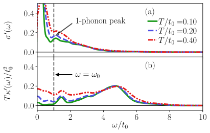
Figure 1: (a) Real part of the optical conductivity for the LL parameters at different temperatures. The arrow illustrates the one-phonon emission peak. (b) Real part of the thermal conductivity for the same parameters. The vertical line shows $\omega=\omega_{0}$.

To better understand the origin of the different parts of the thermal conductivity spectra, we compute the spectra associated with $\hat{J}^{E}_{e-ph}$ from Eq. (6). A comparison of the results using the full current $\hat{J}^{E}$ (solid lines) and $\hat{J}^{E}_{e-ph}$ (dashed lines) is illustrated for two different temperatures in Figs. 2(a) and  2(b). In both cases, the curves almost overlap at high frequencies, implying that the high-frequency structures result from the term in $\hat{J}^{E}$ proportional to $\gamma$, that is, $\hat{J}^{E}_{e-ph}$. We attribute this to the high-energy processes induced by the coupling to the phonons, whereas the optical conductivity is limited by the number of phonons present (at low $T/\omega_{0}$, the spectra are dominated by phonon-emission processes). We also see that the resonance starting at $\omega/t_{0}=1$ can be completely attributed to the $\hat{J}^{E}_{e-ph}$ term. The black dashed line in Fig. 2 is calculated with $L=20$, and apart from very low frequencies, the spectra are almost indistinguishable.

At small $\omega/t_{0}$, the spectra associated with $\hat{J}^{E}$ and $\hat{J}^{E}_{e-ph}$ start to deviate from each other, which signals that $\hat{J}^{E}_{e}$ starts to play a more important role. This also becomes more prominent at higher temperatures, and we attribute a significant portion of the DC thermal conductivity to $\hat{J}^{E}_{e}$ supp-mat .

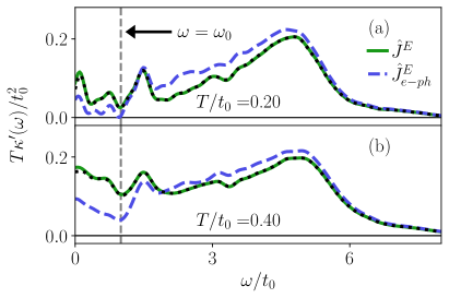
Figure 2: (a) Real part of the thermal conductivity for the LL regime at $T/t_{0}=0.2$. (b) Same as (a) but at $T/t_{0}=0.4$. The solid lines are calculated using $\hat{J}^{E}$ from Eq. (4) and the dashed lines using $\hat{J}^{E}_{e-ph}$ from Eq. (6). The black dotted line shows calculations using $\hat{J}^{E}$ but with $L=20$. The vertical line shows $\omega=\omega_{0}$.

Results: CDW regime. We use $L=10$ unless stated otherwise, and the Fourier transformation is done with $\eta=0.4/(4\pi)$. The corresponding optical conductivities are depicted in Fig. 3(a). For the polaron, it is well established (see, Refs. Reik_67 ; emin_93 ; schubert_05 ; fratini_06 ; jansen22 ), that the optical conductivity spectra are close to an asymmetric Gaussian centered around $2E_{P}=2\gamma^{2}/\omega_{0}$. For the Holstein dimer ($L=2$), this can be interpreted as a transition from the lower to the excited Born-Oppenheimer (BO) surface Born_27 ; Born_54 (BO surfaces are shown in supp-mat ) at a fixed phonon configuration, however, the qualitative picture remains valid for larger systems as well, see, e.g., Refs. jansen22 ; schubert_05 ; fratini_06 . Furthermore, a thermally activated transition for the polaron occurs at $\omega\approx 2t_{0}$ schubert_05 , which can be explained using the BO surfaces as a transition at $\expectationvalue*{\hat{X}_{1}-\hat{X}_{2}}\approx 0$.

In Fig. 3(a), we see that for the selected parameters, the polaron properties carry over to half filling. The center of the spectrum is close to $2E_{P}$ (dotted gray lines) and the thermally activated resonance is clearly visible (dashed line). Note that this peak is also seen for classical phonons, studied in Ref. weber_16 , and has been suggested to be related to finite-temperature disorder physics of noninteracting electrons. Furthermore, it was also discussed in the context of the displaced Drude peak in Ref. fratini_21 .

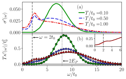
Figure 3: (a) Real part of the optical conductivity for the CDW regime at different temperatures. (b) Real part of the thermal conductivity for the same parameters. The symbols in (b) show the thermal conductivity calculated using $\hat{J}^{E}_{e-ph}$ from Eq. (6). We only plot every 15th point of the $\hat{J}^{E}_{e-ph}$ data for clarity. The dashed vertical line illustrates $\omega=2t_{0}$ and the dotted vertical line $\omega=2E_{P}$. The inset in (b) shows the data for $T/t_{0}=1.0$ as a red solid line for $\hat{J}^{E}$ and a black dotted line for $\hat{J}^{E}_{e-ph}$.

The thermal conductivity calculated with $\hat{J}^{E}_{e-ph}$ and $\hat{J}^{E}$ is shown in Fig. 3(b). The spectra look very similar to those of the optical conductivity, suggesting that they are dominated by small-polaron physics. For the Holstein dimer, $\hat{J}^{E}=\hat{J}^{E}_{e-ph}$, and in the semi-classical approach underlying the BO picture where the phonon states are eigenstates of $\hat{X}_{i}$, one would just expect a rescaled optical conductivity. Our data indicate that the picture is qualitatively correct, but with some notable differences. For example, the center of the spectra is shifted to $\omega>2E_{P}$, and the thermally activated resonance appears as a shoulder peak at $T/t_{0}=1.0$ [inset in Fig. 3(b)]. The data presented in this figure establish that the spectrum mainly results from $\hat{J}^{E}_{e-ph}$ (symbols) for all frequencies visible on the used scale. Thus, the main features can be traced to Holstein-dimer physics.

We next demonstrate that our data can be used to extract DC quantities. In the main text, we focus on $\sigma^{\prime}_{\textrm{DC}}$, while results for $\kappa^{\prime}_{\textrm{DC}}$ are presented in supp-mat . We first demonstrate that for the selected parameters, the time-dependent correlation function quickly decays to zero [see Fig. 4(a)]. Some oscillations can be seen at later times, but they decrease with system size, and $\eta$ is chosen such that the conductivity should be independent thereof [the black dashed line in the inset in Fig. 4(a) shows the correlation function weighted with $e^{-\eta(tt_{0})^{2}}$]. $\sigma^{\prime}_{\textrm{DC}}$ is then obtained as the zeroth component of the Fourier transformed charge current-current correlation function, see Eq. (9).

In systems with small polarons, $\sigma^{\prime}_{\textrm{DC}}$ increases due to thermally activated hopping. As demonstrated in Fig. 4(b), this picture remains valid at half filling. For small polarons, an analytical expression for the resistivity can be derived Bogomolov_69 ; emin_69 ; austin_01

$$\rho_{P}=\rho_{0}Te^{(0.5E_{P}-t_{0})/T}\,.$$ (10)

In Fig. 4(b), we show $\sigma^{\prime}_{\textrm{DC}}$ as a function of temperature. By fitting the inverse of Eq. (10) with $\rho_{0}$ as the fitting parameter to our data, we obtain a very good agreement, and further confirm the importance of small-polaron transport in the system, even at half filling. At large temperatures, the residual finite-size effects are consistent with the remaining $L$-dependence in the autocorrelators [see the inset of Fig. 4(a)]. Note that the error bars in Fig. 4(b) result from comparing data with $\eta=0.2/(4\pi)$ and $\eta=0.6/(4\pi)$ and taking the maximum difference to the $\eta=0.4/(4\pi)$ data at each point. By comparison to state-of-the-art numerical results for one-dimensional spin systems huang_13 ; steinigeweg_15 , we conclude that our method reaches comparably low temperatures yet for much larger local Hilbert spaces.

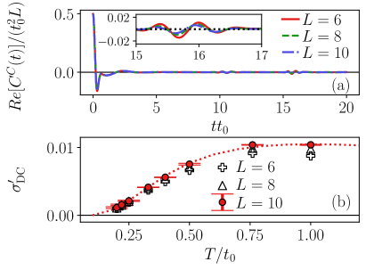
Figure 4: (a) Time-dependent charge current-current correlation functions for the CDW parameters at $T/t_{0}=1.0$ and different system sizes $L$. The inset shows the oscillations at times $15\leq tt_{0}\leq 17$ on a smaller scale. The black dotted line in the inset shows the data weighted with $e^{-\eta(tt_{0})^{2}}$ with $\eta=0.4/(4\pi)$. (b) DC optical conductivity calculated for the same parameters via Eq. (9). The error bars are calculated by varying $\eta$ (see the main text for details). The dotted line is a fit of $\rho_{P}^{-1}$ from Eq. (10) to the data.

Conclusions. In this letter, we studied the thermal and optical conductivity for the Holstein model at finite temperature and half-filling in the Luttinger-liquid and in the CDW regime. Using state-of-the-art MPS time-evolution techniques and using LBO to efficiently deal with the phonons, we computed the energy and charge current-current correlation functions. From those functions, we extracted the finite-frequency transport coefficients. Despite the enhanced complexity of considering finite filling and the complicated energy-current operator, we succeeded in obtaining results at low-temperatures and investigated the role of different terms of the energy-current operator in the two parameter regimes. In particular, our data reveal the importance of small polarons as energy carriers for parameters with a CDW ground state at these temperatures. We further provided an example where the DC conductivity can be reliably obtained in the CDW regime and we identified features in the spectra due to multiphonon processes.

While the spectra of the optical and the thermal conductivity share some similarities, in particular, in the small-polaron regime, there are also noteworthy differences. In the LL regime, the thermal conductivity acquires a high-frequency feature, not seen for $\sigma^{\prime}(\omega)$, that we attribute to multi-phonon processes. In the CDW regime, the thermal conductivity spectrum has a much larger amplitude, the center of the spectra is shifted to higher frequencies, and the thermally activated resonance can only be distinguished at higher $T/\omega_{0}$. Still, the resemblance to the optical conductivity can be understood by looking at the energy-current operator in the dimer limit. Moreover, we unvelied the contribution of small-polaron physics to the optical conductivity (both at finite and zero frequency) and, in particular, to the thermal conductivity in the CDW regime.

One can directly identify several interesting extensions of our work. First, one would want to systematically study the DC conductivity starting from the limit $\gamma=0$, accounting also for a dispersion of the phonons and non-nonlinearity in the phonon sector. Second, the method can be applied to other models as well szabo_21 . For instance, transport of a Heisenberg chain coupled to phonons has not been explored with MPS methods (see Louis2003 ; Louis2006 for related numerical studies). This might provide new insights into experiments on Heisenberg-chain-like systems Sologubenko_07 ; Hess2019 . A different direction would be to extend the analysis to non-equilibrium quantities, see, e.g., Refs. sentef13 ; kemper_17 ; paeckel_fauseweh_19 ; rincon_21 ; ejima_22 , which might require additional sophisticated matrix-product-based schemes jeckelmann98 ; schroeder_16 ; bischoff_17 ; yang_20 ; koehler20 ; Xu_21 ; mardazad_21 ; moroder_22 .

The data shown in this manuscript are available as ancillary files. The files and a link to the code used can be found on the arXiv.

Acknowledgments. We acknowledge useful discussions with J. Bonc̆a, E. Jeckelmann, and J. Lötfering, and we thank M. Weber for comments on a previous version of the manuscript. This work is funded by the Deutsche Forschungsgemeinschaft (DFG, German Research Foundation) – 217133147, 436382789, 493420525 via SFB 1073 (project B09) and large-equipment grants (GOEGrid cluster). D.J. also acknowledges the support from the Government of Spain (European Union NextGenerationEU PRTR-C17.I1, Severo Ochoa CEX2019-000910-S and TRANQI), Fundació Cellex, Fundació Mir-Puig, and Generalitat de Catalunya (CERCA program).

Supplementary material

Born-Oppenheimer surfaces. For the charge-density-wave (CDW) parameters, some of our results can be understood based on the Born-Oppenheimer Hamiltonian and the Born-Huang formalism Born_27 ; Born_54 . For the Holstein model in the dimer limit, see Ref. jansen22 for the convention we use, the Born-Oppenheimer Hamiltonian becomes

$$\hat{H}^{\rm{BO}}=-t_{0}\bigl{(}\hat{c}_{1}^{{\dagger}}\hat{c}_{2}^{\phantom{{\dagger}}}+\textrm{H.c.}\bigr{)}+\gamma\bigl{[}\bar{q}(\hat{n}_{1}-\hat{n}_{2})\bigr{]}+\frac{1}{2}\bar{q}^{2}\omega_{0}\,,$$ (S.1)

which has the eigenenergies

$$E^{\rm{BO}}_{\pm}=\frac{1}{2}\Bigl{(}\bar{q}^{2}\omega_{0}\pm 2\sqrt{(\gamma\bar{q})^{2}+t_{0}^{2}}\Bigr{)}\,.$$ (S.2)

$E^{\rm{BO}}_{\pm}$ as a function of $\bar{q}$ are plotted in Fig. S1. For our parameters, $\Delta^{\rm{BO}}\approx 2E_{P}$ [up to order $\mathcal{O}(10^{-4})$]. The activation energy $E_{A}/t_{0}=1.125>0.5E_{P}/t_{0}-1=1$ gives the exponent in the DC resistivity and we find that using $E_{A}/t_{0}=0.5E_{P}/t_{0}-1$ gives a better fit of our DC conductivity data to $\rho_{P}$ from Eq. (10) of the main text (relative error for the fitting parameter is $0.01$ instead of $0.03$). At $\bar{q}=0$ $\Bigl{(}\expectationvalue*{\hat{X}_{1}-\hat{X}_{2}}=0\Bigr{)}$, we also see the thermally activated transition with an energy difference $\omega/t_{0}=2$.

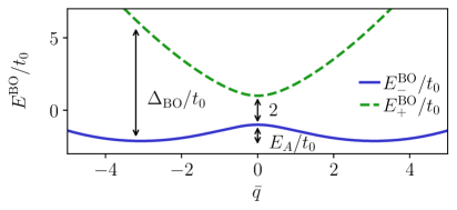
Figure S1: Born-Oppenheimer surface for the CDW parameters. $E_{A}$ is the difference between the minimum and maximum energy of the $E^{\textrm{BO}}_{-}$.

Convergence of the algorithm. In this work, we calculate the time-dependent correlation functions at finite temperatures using matrix-product states (MPSs) with purification verstrate2004 ; schollwock2011density . For the imaginary time-evolution, we use the two-site time-dependent variational principle (TDVP) algorithm haegeman_11 ; haegeman_16 with local basis optimization (LBO) zhang98 .

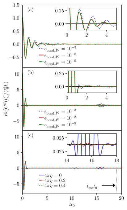
Figure S2: (a) Energy current-current correlation function for the LL parameters, $T/t_{0}=0.4$, and different $\epsilon_{\textrm{bond},\hat{J}^{Q}}$ [see Eq. (S.5)]. (b) Same as (a) but for CDW parameters, $T/t_{0}=0.5$, and $L=10$. (c) Same as (b) but using $\epsilon_{\textrm{bond},\hat{J}^{Q}}=10^{-9}$ and weighting the data with $e^{-\eta(tt_{0})^{2}}$ using different $\eta$. The insets show the corresponding data on a smaller scale. The dotted vertical line in (c) illustrates $t_{\textrm{tot}}t_{0}=19.0$.

When we carry out the singular-value decompositions, we truncate based on the singular values $s_{\eta}$ such that

$$\sum\limits_{\textrm{discarded}\,\eta}s^{2}_{\eta}/(\sum\limits_{\textrm{all}\,\eta}s^{2}_{\eta})<\epsilon_{\textrm{bond}}\,.$$ (S.3)

When we compute the optimal basis in LBO, we truncate the eigenvalues of the reduced density matrix, $w_{\eta}$, such that

$$\sum\limits_{\textrm{discarded}\,\eta}w_{\eta}/(\sum\limits_{\textrm{all}\,\eta}w_{\eta})<\epsilon_{\textrm{LBO}}\,.$$ (S.4)

For all the data shown in this work, we use $\epsilon_{\textrm{LBO}}=\epsilon_{\textrm{bond}}=10^{-9}$ and an imaginary time step $d\tau t_{0}=0.1$. To further verify that the data are converged with respect to varying those parameters, we calculate $\expectationvalue*{[\hat{A}^{Q},\hat{J}^{Q}]}_{T}$ [related to the conductivities via the $f$-sum rule in Eq. (S.7)] for $Q=C$ and $Q=E$, $\expectationvalue*{\hat{H}}$, and $\expectationvalue*{\hat{H}^{2}}$ (the latter two are needed to compute the specific heat of the system). For the Luttinger-liquid (LL) parameters, we found a maximum relative difference for the observable $\expectationvalue*{[\hat{A}^{E},\hat{J}^{E}]}_{T}$ of $0.017$ when using $d\tau t_{0}=0.01$ instead of $d\tau t_{0}=0.1$ for the temperatures used in this work (the maximum difference is for $T/t_{0}=0.1$ and decreasing when $T/t_{0}$ is increased). For the CDW parameters, the maximum relative difference is found for the same observable, and is $0.0062$ for the same change in $d\tau t_{0}$ at $T/t_{0}=1/3$.

During the real-time evolution, we use single-site TDVP haegeman_11 ; haegeman_16 and evolve the component of the state in the physical Hilbert space forwards in time and the component in the ancillary Hilbert space backward in time karrasch2012 ; karrasch2013 ; kennes2016 (note that improvements to single-site TDVP have been suggested, e.g., Refs. yang_20 ; Xu_21 ). Since the algorithm does not increase the bond dimension of the state, we make sure that the dimension is sufficiently large by adapting the truncation parameter of the matrix-product state after applying the current operators $\hat{J}^{Q}$ as matrix-product operators (MPOs). The truncation is based on the singular values such that

$$\sum\limits_{\textrm{discarded}\,\eta}s^{2}_{\eta}/(\sum\limits_{\textrm{all}\,\eta}s^{2}_{\eta})<\epsilon_{\textrm{bond},\hat{J}^{Q}}\,.$$ (S.5)

In Fig. S2, we illustrate how the data converges by varying $\epsilon_{\textrm{bond},\hat{J}^{Q}}$ (Fig. S2(a) for the LL parameters and Fig. S2(b) for the CDW parameters). When $\epsilon_{\textrm{bond},\hat{J}^{Q}}$ is chosen too small, deviations in the correlation functions can be seen. Figure S2(c) shows a correlation function in the CDW regime using different $\eta$. The initial decay is approximately independent thereof, but the later oscillations are significantly damped. We note that in general, convergence of both the correlation functions and the transport coefficients themselves must be monitored carefully.

Since the current operators only act on the physical Hilbert space, we demonstrate how all bonds are impacted by acting on the state with the MPO. We sketch our implementation of the MPS purification ansatz in Fig. S3. We use one separate tensor with both fermionic and bosonic degrees of freedom for each site (physical or ancillary). We then maximally entangle the phononic modes before we apply fermionic creation operators following Ref. barthel_16 to do the calculations in the canonical ensemble.

Figure S3: Matrix-product state consisting of physical (black) and ancillary (red) sites connected to local harmonic oscillators for $L=3$. In our implementation, each site corresponds to a separate tensor. In the purification ansatz, the physical and one ancillary site are maximally entangled at infinite temperature, as illustrated by the thick lines. The other bonds have dimension $d_{\textrm{bond}}=1$. Note that in practice, we work in the canonical ensemble, which does increase the bond dimensions in the system, see Ref. barthel_16 . The numbers indicate the labeling of the bonds shown in Fig. S4.

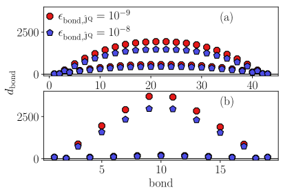
Figure S4: (a) Bond dimensions of the matrix-product state after applying the energy-current operator for the LL parameters with $L=22$ and $T/t_{0}=0.4$, and different $\epsilon_{\textrm{bond},\hat{J}^{Q}}$. (b) Same as (a) but for the CDW parameters with $L=10$ and $T/t_{0}=1.0$. Note that a sketch of the MPS ansatz can be seen in Fig. S3.

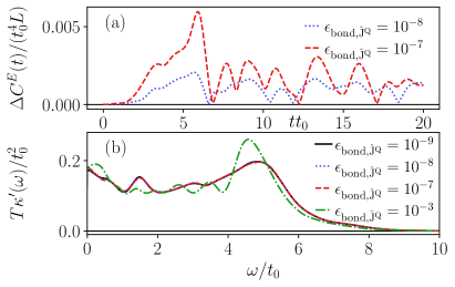
Figure S5: (a) Absolute value of the difference between the energy-energy correlation function calculated with $\epsilon_{\textrm{bond},\hat{J}^{Q}}=10^{-8}$ and $\epsilon_{\textrm{bond},\hat{J}^{Q}}=10^{-9}$ (blue dotted line) and with $\epsilon_{\textrm{bond},\hat{J}^{Q}}=10^{-7}$ and $\epsilon_{\textrm{bond},\hat{J}^{Q}}=10^{-9}$ (red dashed) line (see Eq. (S.6)). (b) Real part of the thermal conductivity for different $\epsilon_{\textrm{bond},\hat{J}^{Q}}$ and $\eta=0.1/(4\pi)$. Note that the influence of $\epsilon_{\textrm{bond},\hat{J}^{Q}}$ on the DC thermal conductivity can be seen in Fig. S8. All calculations are done in the LL regime with $L=22$.

In Fig. S4, we show the bond dimensions after applying the energy current operator. There, one can see that the bond dimension between the originally maximally entangled physical and ancillary sites increases when $\epsilon_{\textrm{bond},\hat{J}^{Q}}$ is varied, especially towards the bulk of the system. The other bond dimensions (away from the edges) also increase, but the difference is not visible on the scales of the figures.

To illustrate the influence of $\epsilon_{\textrm{bond},\hat{J}^{Q}}$ on our data, we plot

$$\Delta C^{E}(t)=\absolutevalue{C^{E}_{\epsilon_{\textrm{bond},\hat{J}^{Q}}=10^{-9}}(t)-C^{E}_{\epsilon_{\textrm{bond},\hat{J}^{Q}}}(t)}\,,$$ (S.6)

where the second $\epsilon_{\textrm{bond},\hat{J}^{Q}}$ is either $10^{-7}$ or $10^{-8}$, in Fig. S5(a). As can be seen, some differences are unavoidable, however, in Fig. S5(b), we show how these differences affect the thermal conductivity. On the scale of interest in this work, the three curves for $\epsilon_{\textrm{bond}}=10^{-7}$, $10^{-8}$, and $10^{-9}$ are indistinguishable. We also show the data for $\epsilon_{\textrm{bond}}=10^{-3}$ to demonstrate that a too large $\epsilon_{\textrm{bond}}$ significantly affects the data. Note that the influence on the DC conductivity can be seen in Fig. S8 and will be discussed later.

Fourier transformation and $f$-sum rule. In this work, the real-time evolution is done up to time $t_{\textrm{tot}}t_{0}$ and we add $4\cdot t_{\textrm{tot}}t_{0}$ zeros to the signal (zero padding). Before the Fourier transformation, the correlation functions are also weighted with the Gaussian damping $e^{-\eta(tt_{0})^{2}}$. To get an estimation of the accuracy of our results and to determine $\eta$, we relate the spectra to thermal expectation values.

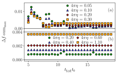
Figure S6: (a) $\Delta f_{\max}$-sum for the thermal conductivity, see Eq. (S.10), as a function of $t_{\textrm{tot}}t_{0}$ for the metallic parameters with $L=22$ and using different broadening parameters $\eta$. (b) Same as (a) but for the CDW parameters and with $L=10$.

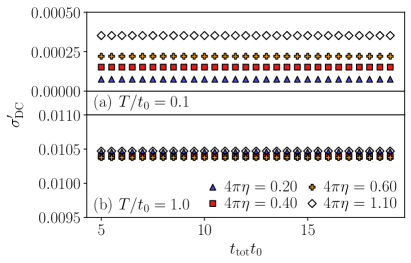
Figure S7: (a) DC optical conductivity in the CDW regime with $L=10$ at $T/t_{0}=0.1$ as a function of $t_{\textrm{tot}}t_{0}$ using different $\eta$. (b) Same as (a) but at $T/t_{0}=1.0$. (a) Illustrates a case where the relative uncertainty is larger than 15%, and the DC conductivity is excluded at this temperature.

The conductivities can be related to the commutator of the current and a polarization $\hat{A}^{Q}=\sum_{j=1}^{L}(j-1)\hat{q}_{j}$ via the $f$-sum rule

$$\begin{split}\int_{0}^{\infty}d\omega\mathcal{L}_{Q}^{\prime}(\omega)=\frac{\pi}{2i}\frac{\expectationvalue*{[\hat{A}^{Q},\hat{J}^{Q}]}_{T}}{L}\,,\end{split}$$ (S.7)

where $[\ldots]$ is the commutator. Note that for the optical conductivity, this becomes

$$\begin{split}\int_{0}^{\infty}d\omega\sigma^{\prime}(\omega)=\frac{-\pi}{2}\frac{E_{\textrm{kin}}}{L}\,,\end{split}$$ (S.8)

where $E_{\textrm{kin}}=\expectationvalue*{-t_{0}\sum_{j=1}^{L-1}(\hat{c}_{j}^{{\dagger}}\hat{c}_{j+1}^{\phantom{{\dagger}}}+\textrm{H.c})}_{T}$. Evaluating both the left and right-hand sides of Eq. (S.7) is then used as a consistency check for our results. To quantify the accuracy of the data, we define the relative difference to be

$$\Delta f\textrm{-sum}=\frac{\absolutevalue*{\int_{0}^{\infty}d\omega\mathcal{L}_{Q}^{\prime}(\omega)-\frac{\pi}{2i}\frac{\expectationvalue*{[\hat{A}^{Q},\hat{J}^{Q}]}_{T}}{L}}}{\absolutevalue*{\frac{\pi}{2i}\frac{\expectationvalue*{[\hat{A}^{Q},\hat{J}^{Q}]}_{T}}{L}}}\,,$$ (S.9)

where the $\mathcal{L}_{Q}^{\prime}(\omega)$ are obtained at the corresponding temperature. In our calculations, we look at $T/t_{0}\in\{0.1,0.2,0.4\}$ in the LL regime for the optical conductivity, $T/t_{0}\in\{0.1,0.2,2/9,0.25,1/3,0.4\}$ for the thermal conductivity, and $T/t_{0}\in\{0.1,0.2,0.4,0.5,1.0\}$ in the CDW regime.

For the thermal conductivity in the LL regime with $\eta=0.1/(4\pi)$ (shown in the main text), we find that $\Delta f\textrm{-sum}$ is at maximum of order $\mathcal{O}(10^{-3})$ for $T/t_{0}=0.1$ and $T/t_{0}=1/3$ and $\mathcal{O}(10^{-4})$ for all other temperatures. For the optical conductivity, the relative accuracy is maximum order $\mathcal{O}(10^{-3})$ for all temperatures. For the optical conductivity in the CDW regime, we also did the calculations for $T/t_{0}=10/13$ (which is shown in the main text) and got consistent results.

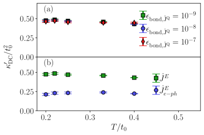
Figure S8: DC thermal conductivity for the LL parameters with $L=22$ and $\eta=0.1/(4\pi)$. (a) Using different truncation parameters $\epsilon_{\textrm{bond},\hat{J}^{Q}}$. (b) Comparison between using $\hat{J}^{E}$ to $\hat{J}^{E}_{e-ph}$ with $\epsilon_{\textrm{bond},\hat{J}^{Q}}=10^{-9}$.

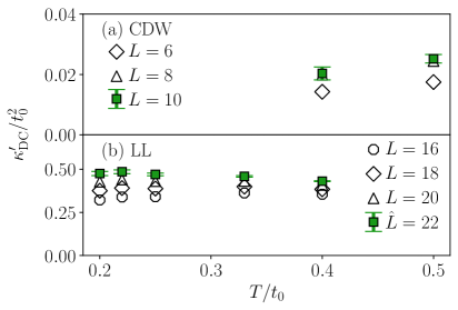
Figure S9: DC thermal conductivity for the CDW (a) and LL (b) parameters calculated with different $L$. In (a), we use $\eta=0.1/(4\pi)$ and in (b) $\eta=0.1/(4\pi)$. The errorbars for $L=10$ in (a) and $L=22$ in (b) are obtained as described in the main text of the Supplementary Material.

In the CDW parameter regime with $\eta=0.4/(4\pi)$ (shown in the main text), we find that $\Delta f\textrm{-sum}$ at maximum of order $\mathcal{O}(10^{-3})$ for both the optical and thermal conductivity at all temperatures.

$\Delta f\textrm{-sum}$ is also used to determine the parameters for the Fourier transformation. We define

$$\Delta f\textrm{-sum}_{\max}=\max_{T}[\Delta f\textrm{-sum}]\,,$$ (S.10)

as the maximum difference for the aforementioned temperatures $T$.

In Figs. S6(a) and S6(b), we show how $\Delta f\textrm{-sum}$ varies for different values of $\eta$ and $t_{\textrm{tot}}t_{0}$. For the LL parameters [Fig. S6(a)], $\Delta f\textrm{-sum}$ fluctuates at small $t_{\textrm{tot}}t_{0}$ but saturates for later times. For the CDW parameters [Fig. S6(b)], $\Delta f\textrm{-sum}$ is roughly independent of $t_{\textrm{tot}}t_{0}$ (note that the times are after the initial decay). However, for small $\eta$, fluctuations can be seen, corresponding to the fluctuations seen in the correlation functions. Since the data are roughly stable (at the desired accuracy for our work) for $\eta=0.4/(4\pi)$, this is used in the main text.

DC conductivity error bars. When computing the DC conductivity, we determine the error bars by computing $\sigma_{\textrm{DC}}^{\prime}$ ($\kappa_{\textrm{DC}}^{\prime}$) for different values of $\eta$. In Fig. S7, we show $\sigma^{\prime}_{\textrm{DC}}$ in the CDW regime (shown in the main text) for different $\eta$ and different $t_{\textrm{tot}}t_{0}$. $\sigma^{\prime}_{\textrm{DC}}$ seems to be roughly independent of $t_{\textrm{tot}}t_{0}$ (when chosen large enough) and $\eta$. The error bars are determined by fixing $\eta=0.1/(4\pi)$ [$\eta=0.4/(4\pi)$] for the LL [CDW] parameters and taking the maximum difference between $\eta=0.1/(4\pi)$ and either $\eta=0.05/(4\pi)$ or $\eta=0.15/(4\pi)$ [$\eta=0.4/(4\pi)$ and either $\eta=0.2/(4\pi)$ or $\eta=0.6/(4\pi)$].

Furthermore, we discard those data points where the relative uncertainty exceeds 15%. For the data shown in the main text, the relative uncertainty is 11% for $T/t_{0}=0.2$ and $<$0.7% for the rest. Figure S7(a) demonstrates an example where the error is of the same magnitude as the quantity and our criterion does not hold, thus the data point is left out.

In Fig. S8(a), we demonstrate the effect of different $\epsilon_{\textrm{bond},\hat{J}^{Q}}$ on the DC conductivity. In the plot, some differences can be seen by changing $\epsilon_{\textrm{bond},\hat{J}^{Q}}$ or $\eta$ (affecting the error bars).

In Fig. S8(b), we compare the DC thermal conductivity computed with $\hat{J}^{E}$ to that computed with $\hat{J}^{E}_{e-ph}$ for the LL parameters. In both cases, we first see a small increase followed by a decay when $T/t_{0}$ gets larger. Furthermore, going from $\hat{J}^{E}$ to $\hat{J}^{E}_{e-ph}$ significantly decreases the DC conductivity.

$\kappa_{\textrm{DC}}^{\prime}$ can be seen in Fig. S9 for the CDW [Fig. S9(a)] and LL [Fig. S9(b)] parameters for different system sizes. Some finite-size effects are still visible, most prominently in the LL regime. We emphasize that our results are comparable to other results for LLs (for spin chains) in the literature huang_13 ; steinigeweg_15 in terms of temperatures reached (where finite-size effects also can be seen), but for the more challenging case with a significantly larger number of local degrees of freedom.

References

- (1) B. Bertini, F. Heidrich-Meisner, C. Karrasch, T. Prosen, R. Steinigeweg, and M. Žnidarič, Finite-temperature transport in one-dimensional quantum lattice models, Rev. Mod. Phys. 93, 025003 (2021).
- (2) V. B. Bulchandani, S. Gopalakrishnan, and E. Ilievski, Superdiffusion in spin chains, J. Stat. Mech. 084001 (2021).
- (3) G. D. Mahan, Many-Particle Physics (Plenum Press, New York, London, 1990).
- (4) C. Hess, Heat transport of cuprate-based low-dimensional quantum magnets with strong exchange coupling, Phys. Rep. 811, 1 (2019).
- (5) L. Perfetti, S. Mitrovic, G. Margaritondo, M. Grioni, L. Forró, L. Degiorgi, and H. Höchst, Mobile small polarons and the Peierls transition in the quasi-one-dimensional conductor , Phys. Rev. B 66, 075107 (2002).
- (6) R. S. Li, L. Yue, Q. Wu, S. X. Xu, Q. M. Liu, Z. X. Wang, T. C. Hu, X. Y. Zhou, L. Y. Shi, S. J. Zhang, D. Wu, T. Dong, and N. L. Wang, Optical spectroscopy and ultrafast pump-probe study of a quasi-one-dimensional charge density wave in CuTe, Phys. Rev. B 105, 115102 (2022).
- (7) S. Schramm, J. Hoffmann, and C. Jooss, Transport and ordering of polarons in CER manganites PrCaMnO, J. Condens. Matter Phys. 20, 395231 (2008).
- (8) G. Saucke, J. Norpoth, C. Jooss, D. Su, and Y. Zhu, Polaron absorption for photovoltaic energy conversion in a manganite-titanate pn heterojunction, Phys. Rev. B 85, 165315 (2012).
- (9) E. Shimshoni, N. Andrei, and A. Rosch, Thermal conductivity of spin-1/2 chains, Phys. Rev. B 68, 104401 (2003).
- (10) A. L. Chernyshev and A. V. Rozhkov, Thermal transport in antiferromagnetic spin-chain materials, Phys. Rev. B 72, 104423 (2005).
- (11) E. Boulat, P. Mehta, N. Andrei, E. Shimshoni, and A. Rosch, Heat transport of clean spin-ladders coupled to phonons: Umklapp scattering and drag, Phys. Rev. B 76, 214411 (2007).
- (12) S. Gangadharaiah, A. L. Chernyshev, and W. Brenig, Thermal drag revisited: Boltzmann versus Kubo, Phys. Rev. B 82, 134421 (2010).
- (13) C. Bartsch and W. Brenig, Thermal drag in spin ladders coupled to phonons, Phys. Rev. B 88, 214412 (2013).
- (14) A. L. Chernyshev and W. Brenig, Thermal conductivity in two-dimensional antiferromagnets: Role of phonon scattering, Phys. Rev. B 92, 054409 (2015).
- (15) A. L. Chernyshev and A. V. Rozhkov, Heat transport in spin chains with weak spin-phonon coupling, Phys. Rev. Lett. 116, 017204 (2016).
- (16) B. Kressdorf, T. Meyer, A. Belenchuk, O. Shapoval, M. ten Brink, S. Melles, U. Ross, J. Hoffmann, V. Moshnyaga, M. Seibt, P. Blöchl, and C. Jooss, Room-temperature hot-polaron photovoltaics in the charge-ordered state of a layered perovskite oxide heterojunction, Phys. Rev. Applied 14, 054006 (2020).
- (17) J. Amarel, D. Belitz, and T. R. Kirkpatrick, Exact solution of the Boltzmann equation for low-temperature transport coefficients in metals. I. Scattering by phonons, antiferromagnons, and helimagnons, Phys. Rev. B 102, 214306 (2020).
- (18) J. Amarel, D. Belitz, and T. R. Kirkpatrick, Rigorous results for the electrical conductivity due to electron–phonon scattering, J. Math. Phys. 62, 023301 (2021).
- (19) S. Fratini, F. de Pasquale, and S. Ciuchi, Optical absorption from a nondegenerate polaron gas, Phys. Rev. B 63, 153101 (2001).
- (20) S. Fratini and S. Ciuchi, Dynamical mean-field theory of transport of small polarons, Phys. Rev. Lett. 91, 256403 (2003).
- (21) S. Fratini and S. Ciuchi, Optical properties of small polarons from dynamical mean-field theory, Phys. Rev. B 74, 075101 (2006).
- (22) K. Louis and C. Gros, Quantum Monte Carlo simulation for the conductance of one-dimensional quantum spin systems, Phys. Rev. B 68, 184424 (2003).
- (23) A. S. Mishchenko, N. Nagaosa, N. V. Prokof’ev, A. Sakamoto, and B. V. Svistunov, Optical conductivity of the Fröhlich polaron, Phys. Rev. Lett. 91, 236401 (2003).
- (24) A. S. Mishchenko, N. Nagaosa, Z.-X. Shen, G. De Filippis, V. Cataudella, T. P. Devereaux, C. Bernhard, K. W. Kim, and J. Zaanen, Charge dynamics of doped holes in high cuprate superconductors: A clue from optical conductivity, Phys. Rev. Lett. 100, 166401 (2008).
- (25) A. S. Mishchenko, N. Nagaosa, G. De Filippis, A. de Candia, and V. Cataudella, Mobility of Holstein polaron at finite temperature: An unbiased approach, Phys. Rev. Lett. 114, 146401 (2015).
- (26) M. Weber and J. K. Freericks, Real-time evolution of static electron-phonon models in time-dependent electric fields, Phys. Rev. E 105, 025301 (2022).
- (27) U. Schollwöck, The density-matrix renormalization group in the age of matrix product states, Ann. Phys. (N. Y.) 326, 96 (2011).
- (28) C. Zhang, E. Jeckelmann, and S. R. White, Density matrix approach to local Hilbert space reduction, Phys. Rev. Lett. 80, 2661 (1998).
- (29) C. Guo, A. Weichselbaum, J. von Delft, and M. Vojta, Critical and strong-coupling phases in one- and two-bath spin-boson models, Phys. Rev. Lett. 108, 160401 (2012).
- (30) C. Brockt, F. Dorfner, L. Vidmar, F. Heidrich-Meisner, and E. Jeckelmann, Matrix-product-state method with a dynamical local basis optimization for bosonic systems out of equilibrium, Phys. Rev. B 92, 241106 (2015).
- (31) J. Stolpp, J. Herbrych, F. Dorfner, E. Dagotto, and F. Heidrich-Meisner, Charge-density-wave melting in the one-dimensional Holstein model, Phys. Rev. B 101, 035134 (2020).
- (32) D. Jansen, J. Bonča, and F. Heidrich-Meisner, Finite-temperature density-matrix renormalization group method for electron-phonon systems: Thermodynamics and Holstein-polaron spectral functions, Phys. Rev. B 102, 165155 (2020).
- (33) D. Jansen, J. Bonča, and F. Heidrich-Meisner, Finite-temperature optical conductivity with density-matrix renormalization group methods for the Holstein polaron and bipolaron with dispersive phonons, Phys. Rev. B 106, 155129 (2022).
- (34) F. Verstraete, J. J. García-Ripoll, and J. I. Cirac, Matrix product density operators: Simulation of finite-temperature and dissipative systems, Phys. Rev. Lett. 93, 207204 (2004).
- (35) T. Barthel, U. Schollwöck, and S. R. White, Spectral functions in one-dimensional quantum systems at finite temperature using the density matrix renormalization group, Phys. Rev. B 79, 245101 (2009).
- (36) T. Barthel, U. Schollwöck, and S. Sachdev, Scaling of the thermal spectral function for quantum critical bosons in one dimension, arXiv:1212.3570 (2012).
- (37) T. Barthel, Precise evaluation of thermal response functions by optimized density matrix renormalization group schemes, New J. Phys. 15, 073010 (2013).
- (38) C. Karrasch, J. H. Bardarson, and J. E. Moore, Finite-temperature dynamical density matrix renormalization group and the Drude weight of spin- chains, Phys. Rev. Lett. 108, 227206 (2012).
- (39) C. Karrasch, J. H. Bardarson, and J. E. Moore, Reducing the numerical effort of finite-temperature density matrix renormalization group calculations, New J. Phys. 15, 083031 (2013).
- (40) D. Kennes and C. Karrasch, Extending the range of real time density matrix renormalization group simulations, Comput. Phys. Commun. 200, 37 (2016).
- (41) T. Barthel, Matrix product purifications for canonical ensembles and quantum number distributions, Phys. Rev. B 94, 115157 (2016).
- (42) S. Paeckel, T. Köhler, A. Swoboda, S. R. Manmana, U. Schollwöck, and C. Hubig, Time-evolution methods for matrix-product states, Ann. Phys. (N. Y.) 411, 167998 (2019).
- (43) M. Quijada, J. Černe, J. R. Simpson, H. D. Drew, K. H. Ahn, A. J. Millis, R. Shreekala, R. Ramesh, M. Rajeswari, and T. Venkatesan, Optical conductivity of manganites: Crossover from Jahn-Teller small polaron to coherent transport in the ferromagnetic state, Phys. Rev. B 58, 16093 (1998).
- (44) C. Hartinger, F. Mayr, A. Loidl, and T. Kopp, Polaronic excitations in colossal magnetoresistance manganite films, Phys. Rev. B 73, 024408 (2006).
- (45) S. Mildner, J. Hoffmann, P. E. Blöchl, S. Techert, and C. Jooss, Temperature- and doping-dependent optical absorption in the small-polaron system , Phys. Rev. B 92, 035145 (2015).
- (46) D. G. Cahill and R. O. Pohl, Thermal conductivity of amorphous solids above the plateau, Phys. Rev. B 35, 4067 (1987).
- (47) C. A. Paddock and G. L. Eesley, Transient thermoreflectance from thin metal films, J. Appl. Phys. 60, 285 (1986).
- (48) A. J. Schmidt, R. Cheaito, and M. Chiesa, A frequency-domain thermoreflectance method for the characterization of thermal properties, Rev. Sci. Instrum. 80, 094901 (2009).
- (49) T. Holstein, Studies of polaron motion: Part I. The molecular-crystal model, Ann. Phys. (N. Y.) 8, 325 (1959).
- (50) T. Holstein, Studies of polaron motion: Part II. The “small” polaron, Ann. Phys. (N. Y.) 8, 343 (1959).
- (51) J. E. Hirsch and E. Fradkin, Phase diagram of one-dimensional electron-phonon systems. II. The molecular-crystal model, Phys. Rev. B 27, 4302 (1983).
- (52) R. J. Bursill, R. H. McKenzie, and C. J. Hamer, Phase diagram of the one-dimensional Holstein model of spinless fermions, Phys. Rev. Lett. 80, 5607 (1998).
- (53) C. E. Creffield, G. Sangiovanni, and M. Capone, Phonon softening and dispersion in the 1D Holstein model of spinless fermions, Eur. Phys. J. B 44, 175 (2005).
- (54) C. Franchini, M. Reticcioli, M. Setvin, and U. Diebold, Polarons in materials, Nat. Rev. Mater. 6, 560 (2021).
- (55) M. Capone, W. Stephan, and M. Grilli, Small-polaron formation and optical absorption in Su-Schrieffer-Heeger and Holstein models, Phys. Rev. B 56, 4484 (1997).
- (56) C. Zhang, E. Jeckelmann, and S. R. White, Dynamical properties of the one-dimensional Holstein model, Phys. Rev. B 60, 14092 (1999).
- (57) G. Schubert, G. Wellein, A. Weisse, A. Alvermann, and H. Fehske, Optical absorption and activated transport in polaronic systems, Phys. Rev. B 72, 104304 (2005).
- (58) J. Loos, M. Hohenadler, A. Alvermann, and H. Fehske, Optical conductivity of polaronic charge carriers, J. Phys. Condens. Matter 19, 236233 (2007).
- (59) G. Wellein and H. Fehske, Self-trapping problem of electrons or excitons in one dimension, Phys. Rev. B 58, 6208 (1998).
- (60) G. L. Goodvin, A. S. Mishchenko, and M. Berciu, Optical conductivity of the Holstein polaron, Phys. Rev. Lett. 107, 076403 (2011).
- (61) M. Weber, F. F. Assaad, and M. Hohenadler, Thermodynamic and spectral properties of adiabatic Peierls chains, Phys. Rev. B 94, 155150 (2016).
- (62) J. Bonča and S. A. Trugman, Dynamic properties of a polaron coupled to dispersive optical phonons, Phys. Rev. B 103, 054304 (2021).
- (63) S. Fratini and S. Ciuchi, Displaced Drude peak and bad metal from the interaction with slow fluctuations., SciPost Phys. 11, 039 (2021).
- (64) H. Rezania and F. Taherkhani, Polaron effects on the thermal conductivity of zigzag carbon nanotubes, Solid State Commun. 152, 1776 (2012).
- (65) M. Weber, F. F. Assaad, and M. Hohenadler, Thermal and quantum lattice fluctuations in Peierls chains, Phys. Rev. B 98, 235117 (2018).
- (66) eprint Supplementary material, including a discussion of Born-Oppenheimer surfaces, convergence of the algo- rithm, details of the Fourier transformation and analysis of -sum rule, extraction of the DC conductivity and estimation of error bars.
- (67) R. Kubo, Statistical-mechanical theory of irreversible processes. I. general theory and simple applications to magnetic and conduction problems, J. Phys. Soc. Jpn. 12, 570 (1957).
- (68) J. M. Luttinger, Theory of thermal transport coefficients, Phys. Rev. 135, A1505 (1964).
- (69) N. Pottier, Nonequilibrium Statistical Physics: Linear Irreversible Processes (Oxford University Press, Oxford, 2010).
- (70) C. Schönle, D. Jansen, F. Heidrich-Meisner, and L. Vidmar, Eigenstate thermalization hypothesis through the lens of autocorrelation functions, Phys. Rev. B 103, 235137 (2021).
- (71) Y. Huang, C. Karrasch, and J. E. Moore, Scaling of electrical and thermal conductivities in an almost integrable chain, Phys. Rev. B 88, 115126 (2013).
- (72) R. Steinigeweg, J. Gemmer, and W. Brenig, Spin and energy currents in integrable and nonintegrable spin- chains: A typicality approach to real-time autocorrelations, Phys. Rev. B 91, 104404 (2015).
- (73) M. Rigol and B. S. Shastry, Drude weight in systems with open boundary conditions, Phys. Rev. B 77, 161101 (2008).
- (74) J. Haegeman, J. I. Cirac, T. J. Osborne, I. Pižorn, H. Verschelde, and F. Verstraete, Time-dependent variational principle for quantum lattices, Phys. Rev. Lett. 107, 070601 (2011).
- (75) J. Haegeman, C. Lubich, I. Oseledets, B. Vandereycken, and F. Verstraete, Unifying time evolution and optimization with matrix product states, Phys. Rev. B 94, 165116 (2016).
- (76) M. Fishman, S. R. White, and E. M. Stoudenmire, The ITensor Software Library for Tensor Network Calculations (C++ version), SciPost Phys. Codebases 4 (2022).
- (77) H. Reik and D. Heese, Frequency dependence of the electrical conductivity of small polarons for high and low temperatures, J. Phys. Chem. Solids 28, 581 (1967).
- (78) D. Emin, Optical properties of large and small polarons and bipolarons, Phys. Rev. B 48, 13691 (1993).
- (79) M. Born and R. Oppenheimer, Zur Quantentheorie der Molekeln, Ann. Phys. (Leipzig) 389, 457 (1927).
- (80) M. Born and K. Huang, Dynamical theory of crystal lattices (Clarendon press, Oxford, 1954).
- (81) V. N. Bogomolov, Y. A. Firsov, E. K. Kudinov, and D. N. Mirlin, On the experimental observation of small polarons in rutile (TiO2), physica status solidi (b) 35, 555 (1969).
- (82) D. Emin and T. Holstein, Studies of small-polaron motion IV. Adiabatic theory of the Hall effect, Ann. Phys. (N. Y.) 53, 439 (1969).
- (83) I. G. Austin and N. F. Mott, Polarons in crystalline and non-crystalline materials, Adv. Phys. 50, 757 (2001).
- (84) A. Szabó, S. A. Parameswaran, and A. Gopalakrishnan, High-temperature transport and polaron speciation in the anharmonic Holstein model, arXiv:2110.10170 (2021).
- (85) K. Louis, P. Prelovšek, and X. Zotos, Thermal conductivity of one-dimensional spin- systems coupled to phonons, Phys. Rev. B 74, 235118 (2006).
- (86) A. V. Sologubenko, T. Lorenz, H. R. Ott, and A. Freimuth, Thermal conductivity via magnetic excitations in spin-chain materials, J. Low Temp. Phys. 147, 387 (2007).
- (87) M. Sentef, A. F. Kemper, B. Moritz, J. K. Freericks, Z.-X. Shen, and T. P. Devereaux, Examining electron-boson coupling using time-resolved spectroscopy, Phys. Rev. X 3, 041033 (2013).
- (88) A. F. Kemper, M. A. Sentef, B. Moritz, T. P. Devereaux, and J. K. Freericks, Review of the theoretical description of time-resolved angle-resolved photoemission spectroscopy in electron-phonon mediated superconductors, Ann. Phys. (Berl.) 529, 1600235 (2017).
- (89) S. Paeckel, B. Fauseweh, A. Osterkorn, T. Köhler, D. Manske, and S. R. Manmana, Detecting superconductivity out of equilibrium, Phys. Rev. B 101, 180507 (2020).
- (90) J. Rincón and A. E. Feiguin, Nonequilibrium optical response of a one-dimensional Mott insulator, Phys. Rev. B 104, 085122 (2021).
- (91) S. Ejima, F. Lange, and H. Fehske, Nonequilibrium dynamics in pumped Mott insulators, Phys. Rev. Research 4, L012012 (2022).
- (92) E. Jeckelmann and S. R. White, Density-matrix renormalization-group study of the polaron problem in the Holstein model, Phys. Rev. B 57, 6376 (1998).
- (93) F. A. Y. N. Schröder and A. W. Chin, Simulating open quantum dynamics with time-dependent variational matrix product states: Towards microscopic correlation of environment dynamics and reduced system evolution, Phys. Rev. B 93, 075105 (2016).
- (94) J.-M. Bischoff and E. Jeckelmann, Density-matrix renormalization group method for the conductance of one-dimensional correlated systems using the Kubo formula, Phys. Rev. B 96, 195111 (2017).
- (95) M. Yang and S. R. White, Time-dependent variational principle with ancillary Krylov subspace, Phys. Rev. B 102, 094315 (2020).
- (96) T. Köhler, J. Stolpp, and S. Paeckel, Efficient and flexible approach to simulate low-dimensional quantum lattice models with large local Hilbert spaces, SciPost Phys. 10, 58 (2021).
- (97) Y. Xu, Z. Xie, X. Xie, U. Schollwöck, and H. Ma, Stochastic adaptive single-site time-dependent variational principle, JACS Au 2, 335 (2022).
- (98) S. Mardazad, Y. Xu, X. Yang, M. Grundner, U. Schollwöck, H. Ma, and S. Paeckel, Quantum dynamics simulation of intramolecular singlet fission in covalently linked tetracene dimer, J. Chem. Phys. 155, 194101 (2021).
- (99) M. Moroder, M. Grundner, F. Damanet, U. Schollwöck, S. Mardazad, S. Flannigan, T. Köhler, and S. Paeckel, Stable bipolarons in open quantum systems, Phys. Rev. B 107, 214310 (2023).