Casimir-Polder interaction with Chern-Simons boundary layers

Abstract

Green functions scattering method is generalized to consider mixing of electromagnetic polarizations after reflection from the plane boundary between different media and applied to derivation of the Casimir-Polder potential in systems with Chern-Simons plane boundary layers. The method is first applied to derive the Casimir-Polder potential of an anisotropic atom in the presence of a Chern-Simons plane boundary layer on a dielectric half-space. Then a general result for the Casimir-Polder potential of an anisotropic atom between two dielectric half-spaces with Chern-Simons plane parallel boundary layers is derived. The Casimir-Polder potential of an anisotropic atom between two Chern-Simons plane parallel layers in vacuum is expressed through special functions. Novel P-odd three-body vacuum effects are discovered and analyzed in the system of two Chern-Simons plane parallel layers and a neutral atom in its ground state between the layers. Remarkably, P-odd three-body vacuum effects arising due to $180$ degree rotation of one of the Chern-Simons layers can be verified in experiments with neutral atoms having QED dipole interaction with an electromagnetic field.

I Introduction

The Casimir effect [1, 2] is a quantum effect which studies interaction between macroscopic objects in their ground state. Interaction between two dielectric half-spaces separated by a vacuum slit is determined by the Lifshitz formula [3]. Theoretical study of the Casimir effect has received new possibilities in the framework of scattering approach, the formalism has been effectively applied to non-flat geometries including diffraction gratings [4, 5, 6], spheres and cylinders [7, 8, 9, 10, 11]. One can find details of theoretical and experimental research in various reviews and books on the subject [12, 13, 14, 15, 16, 17, 18, 19, 20, 21, 22, 23, 24, 25, 26, 27, 28, 29, 30, 31, 32].

Chern-Simons action modifies the Casimir interaction essentially, its study within 2+1 Abelian electrodynamics with Chern-Simons term has been started in Ref. [33] where the Maxwell-Chern-Simons electrodynamics has a massive spin-1 excitation. Chern-Simons constants of the layers are dimensionless in 3+1 case. Rigid nonpenetrable boundary conditions modified by a Chern-Simons term in 3+1 case have been considered in Refs. [34, 35], the Hall conductivity is not described by these conditions. The Casimir energy of two flat Chern-Simons layers in vacuum has been derived in Refs. [36, 37], Casimir attraction and repulsion due to Chern-Simons boundary layers on dielectric and metal half-spaces have been studied in Refs. [38, 39].

The Casimir-Polder potential for an anisotropic atom is obtained by direct application of quantum electrodynamics in the second order perturbation theory [40, 41, 42, 43, 44]. The Casimir-Polder effect for conducting planes has been considered in Refs.[45, 46], the Casimir-Polder effect for conducting planes with a tensorial conductivity [47] has been considered in Refs.[12, 48, 49]. The Casimir-Polder potential of a neutral anisotropic atom in the presence of a plane Chern-Simons layer has been derived in Ref. [50], charge-parity violating effects due to Chern-Simons layer have been investigated in Ref. [51].

In the low-energy effective theory of topological insulators there is a term proportional to $\theta\vec{E}\vec{H}$ in addition to the standard electromagnetic energy density, this action can be integrated over the volume of topological insulator into Chern-Simons action at the boundary. The parameter $a$ of Chern-Simons action is quantized in this case as follows: $a=\alpha\theta/(2\pi)$, $\theta=(2m+1)\pi$, $\alpha$ is QED fine structure constant, $m$ is an integer number [52]. Various aspects of the Casimir interaction of topological insulators have been studied in literature [53, 54, 55, 56, 57, 58].

Theoretical description of Chern insulators [59, 60, 61] is given in a non-dispersive case by Chern-Simons action with the parameter $a=C\alpha$, $C$ is a Chern number - topological invariant giving the winding number of a map from a two-dimensional torus to a two-dimensional unit sphere. The Casimir interaction of Chern insulators is studied in Refs. [37, 62, 63].

Quantum Hall layers in external magnetic field also lead to a quantized Casimir force, the parameter of the Chern-Simons action $a=\nu\alpha$, $\nu$ is an integer or a fractional number characterizing the plateau of the quantum Hall effect [38, 64, 65].

The Casimir repulsion attracts a special attention in the Casimir effect research, repulsion is a promising regime from the point of view of technology. Rotation of polarization after reflection of the electromagnetic wave from the Chern-Simons plane layer is an important property which leads to regimes of attraction and repulsion in the Casimir pressure between two Chern-Simons plane parallel layers in vacuum and on boundaries of dielectrics or metals [36, 37, 38, 39]. Repulsive Casimir pressure has not been investigated experimentally in this geometry so far.

A complementary way to study the Casimir effect is a local probe of vacuum by a neutral atom in its ground state. It is tempting to study vacuum between two Chern-Simons plane parallel layers locally due to intriguing properties of this system. This paper fills the gap in an important direction of local study of vacuum in geometry of two Chern-Simons layers. Analytic results for the Casimir-Polder potential of an anisotropic atom between two Chern-Simons plane parallel layers in vacuum and on boundaries of dielectric half-spaces are derived for the first time in the present work.

Recently the formalism based on Green functions scattering has been introduced [12]; in this approach one evaluates electric, magnetic Green functions and the Casimir pressure in an explicit gauge-invariant derivation. In Ref.[12] we have derived the Casimir pressure and the Casimir-Polder potential in systems without rotation of polarizations after reflection of electromagnetic waves from boundaries between different media.

In the present paper we develop a principal generalization of the Green functions scattering approach to a general case of reflection from plane boundaries. In the presence of several Chern-Simons layers one can not express the Casimir-Polder potential in terms of two reflection coefficients (for TE and TM modes) even for a diagonal tensor of atomic polarizability due to rotation of TE and TM polarizations after reflection of the electromagnetic field from each Chern-Simons layer. The matrix of reflection coefficients is non-diagonal in this case [37, 38]. Derivation of the Casimir-Polder potential in the presence of several Chern-Simons layers has required a development of a novel technique presented in this paper. We derive new formulas for the Casimir-Polder potentials for all systems considered in this paper. We also discover and investigate novel three-body vacuum effects in atom - two layers system due to $180$ degree rotation of one of the layers.

We proceed as follows. In Section II we write expressions for the field of a point dipole in vacuum in terms of electric and magnetic fields following Ref.[12] and generalize Green functions scattering formalism to the important case of non-diagonal reflection matrices. Then we derive the result for the Casimir-Polder potential of an anisotropic atom in the presence of a Chern-Simons plane boundary layer on a dielectric half-space. In Section III we derive a general result for the Casimir-Polder potential of an anisotropic atom between two dielectric half-spaces with Chern-Simons plane parallel boundary layers. In Section IV we derive results for the Casimir-Polder potential of an anisotropic atom between two Chern-Simons plane parallel layers in vacuum expressed through Lerch transcendent functions and polylogarithms. Section V is devoted to the analysis of P-odd three-body vacuum effects, experiments to measure the Casimir-Polder potential in the slit are outlined.

Magnetic permeability of materials $\mu=1$ throughout the text. We use $\hbar=c=1$ and Heaviside-Lorentz units.

II The Casimir-Polder Potential of an Anisotropic Atom above a Dielectric Half-Space with Chern-Simons boundary layer

Green functions scattering method has been introduced in Ref.[12] where it has been applied to derivation of various classical results for the Casimir-Polder potential and the Casimir pressure in geometries with plane boundaries, an explicit gauge-invariant derivation of results has been worked out. All results in Ref.[12] are expressed in terms of reflection coefficients for TE and TM modes for problems when no mixing of TE and TM modes is present after reflection of the electromagnetic wave from the plane boundary between different media.

Chern-Simons boundary layer rotates each polarization of the incoming electromagnetic field after reflection from the layer, rotation of polarizations is described in this case by a non-diagonal reflection matrix [37, 38]. Green functions scattering method is generalized in this work to a general non-diagonal reflection problem when applied to derivation of the Casimir-Polder potential. The generalized formalism is developed and presented in detail in this paper.

The result for the Casimir-Polder potential of a neutral anisotropic atom interacting with Chern-Simons plane layer in vacuum is derived in Ref.[50]. In this Section we generalize the result of Ref.[50] and derive the Casimir-Polder potential of a neutral anisotropic atom in its ground state located at a distance $z_{0}$ from a dielectric half-space with a plane Chern-Simons boundary layer.

Consider a dipole source at the point $\mathbf{r^{\prime}}=(0,0,z_{0})$ characterized by electric dipole moment $d^{l}(t)$ with components of the four-current density [50]

$$\rho(t,\mathbf{r}) =-d^{l}(t)\partial_{l}\delta^{3}(\mathbf{r-r^{\prime}})\>,$$ (1)

$$j^{l}(t,\mathbf{r}) =\partial_{t}d^{l}(t)\delta^{3}(\mathbf{r-r^{\prime}})\>.$$ (2)

Exact electric Green function can be found from the electric field part solution of Maxwell equations for the electromagnetic field propagating from a dipole source (1),(2). The scattered electric Green function $D^{E}_{ij}(t_{1}-t_{2},\mathbf{r},\mathbf{r^{\prime}})$ is a difference of the exact electric Green function and the vacuum electric Green function. The Casimir-Polder potential is defined in terms of the scattered electric Green function $D^{E}_{ij}(t_{1}-t_{2},\mathbf{r},\mathbf{r^{\prime}})$ from the source (1),(2) and the atomic polarizability $\alpha_{ij}(t_{1}-t_{2})=i\langle T(\hat{d}_{i}(t_{1}),\hat{d}_{j}(t_{2}))\rangle$ as follows [12]:

$$U(z_{0})=-\int\limits_{0}^{\infty}\frac{d\omega}{2\pi}\alpha^{ij}(i\omega)D^{E}_{ij}(i\omega,\mathbf{r^{\prime}},\mathbf{r^{\prime}}).$$ (3)

From Weyl formula [66]

$$\frac{e^{i\omega|\mathbf{r^{\prime}-r}|}}{4\pi|\mathbf{r^{\prime}-r}|}=i\iint\frac{e^{i(k_{x}(x^{\prime}-x)+k_{y}(y^{\prime}-y)+\sqrt{\omega^{2}-k^{2}_{x}-k^{2}_{y}}(z^{\prime}-z))}}{2\sqrt{\omega^{2}-k^{2}_{x}-k^{2}_{y}}}\frac{dk_{x}dk_{y}}{(2\pi)^{2}}\>,$$ (4)

valid for $z^{\prime}-z>0$, one can write electric and magnetic fields propagating downwards from the dipole source (1),(2) in the form [12]

$$\mathbf{E^{0}}(\omega,\mathbf{r}) =\int\widetilde{\mathbf{N}}(\omega,\mathbf{k_{\parallel}})e^{i\mathbf{k_{\parallel}\cdot r_{\parallel}}}e^{-ik_{z}(z-z_{0})}d^{2}\mathbf{k_{\parallel}},$$ (5)

$$\mathbf{H^{0}}(\omega,\mathbf{r}) =\frac{1}{\omega}\int[\widetilde{\mathbf{k}}\times\widetilde{\mathbf{N}}(\omega,\mathbf{k_{\parallel}})]e^{i\mathbf{k_{\parallel}\cdot r_{\parallel}}}e^{-ik_{z}(z-z_{0})}d^{2}\mathbf{k_{\parallel}},$$ (6)

$$\widetilde{\mathbf{N}}(\omega,\mathbf{k_{\parallel}}) =\frac{i}{8\pi^{2}k_{z}}\left(-(\mathbf{d}\cdot\widetilde{\mathbf{k}})\mathbf{\widetilde{k}}+\omega^{2}\mathbf{d}\right),$$ (7)

where $\mathbf{k_{\parallel}}=(k_{x},k_{y})$, $k_{z}=\sqrt{\omega^{2}-k_{\parallel}^{2}}$, $\mathbf{\widetilde{k}}=(\mathbf{k_{\parallel}},-k_{z})$. Components of the vacuum electric Green function for $z^{\prime}-z>0$ can be determined from (5).

Consider a diffraction problem on a homogeneous dielectric half-space $z<0$ characterized by a dielectric permittivity $\varepsilon(\omega)$ and a plane Chern-Simons boundary layer at $z=0$ described by the action

$$S_{CS}=\frac{a}{2}\int\varepsilon^{z\nu\rho\sigma}A_{\nu}F_{\rho\sigma}\,\,dtdxdy.$$ (8)

To solve a diffraction problem we write electric and magnetic fields for $z>0$ in the form

$$\mathbf{E^{1}}(\omega,\mathbf{r}) =\int\widetilde{\mathbf{N}}(\omega,\mathbf{k_{\parallel}})e^{i\mathbf{k_{\parallel}\cdot r_{\parallel}}}e^{-ik_{z}(z-z_{0})}d^{2}\mathbf{k_{\parallel}}+\int\mathbf{v}(\omega,\mathbf{k_{\parallel}})e^{i\mathbf{k_{\parallel}\cdot r_{\parallel}}}e^{ik_{z}z}d^{2}\mathbf{k_{\parallel}}\>,$$ (9)

$$\mathbf{H^{1}}(\omega,\mathbf{r}) =\frac{1}{\omega}\int[\widetilde{\mathbf{k}}\times\widetilde{\mathbf{N}}(\omega,\mathbf{k_{\parallel}})]e^{i\mathbf{k_{\parallel}\cdot r_{\parallel}}}e^{-ik_{z}(z-z_{0})}d^{2}\mathbf{k_{\parallel}}$$

$$+\frac{1}{\omega}\int[\mathbf{k\times v}(\omega,\mathbf{k_{\parallel})}]e^{i\mathbf{k_{\parallel}\cdot r_{\parallel}}}e^{ik_{z}z}d^{2}\mathbf{k_{\parallel}}\>,$$ (10)

and for $z<0$ in the form

$$\mathbf{E^{2}}(\omega,\mathbf{r}) =\int\mathbf{u}(\omega,\mathbf{k_{\parallel}})e^{i\mathbf{k_{\parallel}\cdot r_{\parallel}}}e^{-iK_{z}z}d^{2}\mathbf{k_{\parallel}}\>,$$ (11)

$$\mathbf{H^{2}}(\omega,\mathbf{r}) =\frac{1}{\omega}\int\left(\mathbf{[k_{\parallel}\times u}(\omega,\mathbf{k_{\parallel})]}-K_{z}\mathbf{[n\times u}(\omega,\mathbf{k_{\parallel})]}\right)e^{i\mathbf{k_{\parallel}\cdot r_{\parallel}}}e^{-iK_{z}z}d^{2}\mathbf{k_{\parallel}}\>$$ (12)

with $K_{z}=\sqrt{\varepsilon(\omega)\omega^{2}-k_{x}^{2}-k_{y}^{2}}$ and $\mathbf{n}=(0,0,1)$. Unknown vector functions $\mathbf{v}(\omega,\mathbf{k_{\parallel}})$ and $\mathbf{u}(\omega,\mathbf{k_{\parallel}})$ can be found from the system of boundary conditions imposed on electric and magnetic fields:

$${\rm div}(\mathbf{E^{1}}-\mathbf{E^{0}})=0,$$ (13)

$${\rm div}\mathbf{E^{2}}=0,$$ (14)

$$E_{x}^{1}|_{z=0}=E_{x}^{2}|_{z=0},$$ (15)

$$E_{y}^{1}|_{z=0}=E_{y}^{2}|_{z=0},$$ (16)

$$H_{x}^{1}|_{z=0+}-H_{x}^{2}|_{z=0-}=2aE_{x}^{1}|_{z=0},$$ (17)

$$H_{y}^{1}|_{z=0+}-H_{y}^{2}|_{z=0-}=2aE_{y}^{1}|_{z=0}.$$ (18)

Boundary conditions (17), (18) have been considered in a study of propagation of a plane electromagnetic wave in a medium with a piecewise constant axion field [67] and in a medium with Chern-Simons layers [68]. Note that the parameter $a$ is proportional to a non-diagonal part of the surface conductivity [58]. With this understanding the frequency dispersion $a(\omega)$ may be considered in boundary conditions (17), (18). To simplify notations we do not write explicitly the frequency $\omega$ in $a(\omega)$ in what follows. In the Casimir-Polder potential formulas we implicitly assume $a(i\omega)$ dependence.

It is convenient to use polar coordinates in two dimensional $(k_{x},k_{y})$ momentum space and local orthogonal basis $\mathbf{e}_{r},\mathbf{e}_{\theta},\mathbf{e}_{z}$ so that $\mathbf{k_{\parallel}}=k_{r}\mathbf{e}_{r}$, $k_{r}=|\mathbf{k_{\parallel}}|$. We write boundary conditions in this basis

$$v_{r}k_{r}+k_{z}v_{z}=0,$$ (19)

$$u_{r}k_{r}-K_{z}u_{z}=0,$$ (20)

$$u_{r}=v_{r}+\widetilde{N}_{r}e^{ik_{z}z_{0}},$$ (21)

$$u_{\theta}=v_{\theta}+\widetilde{N}_{\theta}e^{ik_{z}z_{0}},$$ (22)

$$-k_{z}v_{\theta}+k_{z}\widetilde{N}_{\theta}e^{ik_{z}z_{0}}-K_{z}u_{\theta}=2\omega au_{r},$$ (23)

$$k_{z}v_{r}-k_{r}v_{z}-k_{z}\widetilde{N}_{r}e^{ik_{z}z_{0}}-k_{r}\widetilde{N}_{z}e^{ik_{z}z_{0}}+K_{z}u_{r}+k_{r}u_{z}=2\omega au_{\theta}$$ (24)

and get

$$v_{r} =\biggl{[}-\frac{r_{TM}+a^{2}T}{1+a^{2}T}\widetilde{N}_{r}+\frac{k_{z}}{\omega}\frac{aT}{1+a^{2}T}\widetilde{N}_{\theta}\biggr{]}e^{ik_{z}z_{0}},$$ (25)

$$v_{\theta} =\biggl{[}-\frac{\omega}{k_{z}}\frac{aT}{1+a^{2}T}\widetilde{N}_{r}+\frac{r_{TE}-a^{2}T}{1+a^{2}T}\widetilde{N}_{\theta}\biggr{]}e^{ik_{z}z_{0}},$$ (26)

$$v_{z} =\frac{k_{r}}{k_{z}}\biggl{[}\frac{r_{TM}+a^{2}T}{1+a^{2}T}\widetilde{N}_{r}-\frac{k_{z}}{\omega}\frac{aT}{1+a^{2}T}\widetilde{N}_{\theta}\biggr{]}e^{ik_{z}z_{0}},$$ (27)

where $r_{TM}$, $r_{TE}$ are Fresnel reflection coefficients

$$r_{TM}(\omega,k_{r})=\frac{\varepsilon(\omega)k_{z}-K_{z}}{\varepsilon(\omega)k_{z}+K_{z}}\>,\>\>\>\>\>\>r_{TE}(\omega,k_{r})=\frac{k_{z}-K_{z}}{k_{z}+K_{z}}$$ (28)

and

$$T(\omega,k_{r})=\frac{4k_{z}K_{z}}{(k_{z}+K_{z})(\varepsilon(\omega)k_{z}+K_{z})}.$$ (29)

Note that we omit dependence of reflection and transmission coefficients on $(\omega,k_{r})$ in (25)-(27) for brevity.

At this point it is convenient to define the local matrix $R$ resulting from equations (25), (26):

$$R(a,\varepsilon(\omega),\omega,k_{r})\equiv\frac{1}{1+a^{2}T}\begin{pmatrix}-r_{TM}-a^{2}T&\frac{k_{z}}{\omega}aT\\ -\frac{\omega}{k_{z}}aT&r_{TE}-a^{2}T\par\end{pmatrix}.$$ (30)

To find the reflected part of the electric field one should use rotation between two local bases and make substitutions

$$d_{r} =d_{x}\cos\theta+d_{y}\sin\theta\>,$$ (31)

$$d_{\theta} =d_{x}\sin\theta-d_{y}\cos\theta\>,$$ (32)

$$v_{x} =v_{r}\cos\theta+v_{\theta}\sin\theta\>,$$ (33)

$$v_{y} =v_{r}\sin\theta-v_{\theta}\cos\theta$$ (34)

for every given $\mathbf{k_{\parallel}}$ to the scattered field part of the expression (9) by use of (7), (25), (26), (27). In doing so and noting that

$$\widetilde{N}_{r} =\frac{i}{8\pi^{2}}(k_{z}(d_{x}\cos\theta+d_{y}\sin\theta)+k_{r}d_{z}),$$ (35)

$$\widetilde{N}_{\theta} =\frac{i}{8\pi^{2}}\frac{\omega^{2}}{k_{z}}(d_{x}\sin\theta-d_{y}\cos\theta),$$ (36)

we obtain local contributions to cartesian components of scattered electric Green functions for coinciding arguments at the point of a dipole source:

$$D^{E}_{xx}(\omega,k_{r},\theta,z=z^{\prime}=z_{0})=\frac{i}{8\pi^{2}}\biggl{[}\biggl{(}R_{11}k_{z}\cos\theta+R_{12}\frac{\omega^{2}}{k_{z}}\sin\theta\biggr{)}\cos\theta\\ +\biggl{(}R_{21}k_{z}\cos\theta+R_{22}\frac{\omega^{2}}{k_{z}}\sin\theta\biggr{)}\sin\theta\biggr{]}e^{2ik_{z}z_{0}},$$ (37)

$$D^{E}_{yy}(\omega,k_{r},\theta,z=z^{\prime}=z_{0})=\frac{i}{8\pi^{2}}\biggl{[}\biggl{(}R_{11}k_{z}\sin\theta-R_{12}\frac{\omega^{2}}{k_{z}}\cos\theta\biggr{)}\sin\theta\\ -\biggl{(}R_{21}k_{z}\sin\theta-R_{22}\frac{\omega^{2}}{k_{z}}\cos\theta\biggr{)}\cos\theta\biggr{]}e^{2ik_{z}z_{0}},$$ (38)

$$D^{E}_{zz}(\omega,k_{r},\theta,z=z^{\prime}=z_{0})=-\frac{i}{8\pi^{2}}\frac{k_{r}^{2}}{k_{z}}R_{11}e^{2ik_{z}z_{0}},$$ (39)

$$D^{E}_{xy}(\omega,k_{r},\theta,z=z^{\prime}=z_{0})=\frac{i}{8\pi^{2}}\biggl{[}\biggl{(}R_{11}k_{z}\sin\theta-R_{12}\frac{\omega^{2}}{k_{z}}\cos\theta\biggr{)}\cos\theta\\ +\biggl{(}R_{21}k_{z}\sin\theta-R_{22}\frac{\omega^{2}}{k_{z}}\cos\theta\biggr{)}\sin\theta\biggr{]}e^{2ik_{z}z_{0}},$$ (40)

$$D^{E}_{yx}(\omega,k_{r},\theta,z=z^{\prime}=z_{0})=\frac{i}{8\pi^{2}}\biggl{[}\biggl{(}R_{11}k_{z}\cos\theta+R_{12}\frac{\omega^{2}}{k_{z}}\sin\theta\biggr{)}\sin\theta\\ -\biggl{(}R_{21}k_{z}\cos\theta+R_{22}\frac{\omega^{2}}{k_{z}}\sin\theta\biggr{)}\cos\theta\biggr{]}e^{2ik_{z}z_{0}},$$ (41)

$$D^{E}_{xz}(\omega,k_{r},\theta,z=z^{\prime}=z_{0})=\frac{i}{8\pi^{2}}\biggl{[}R_{11}k_{r}\cos\theta+R_{21}k_{r}\sin\theta\biggr{]}e^{2ik_{z}z_{0}},$$ (42)

$$D^{E}_{zx}(\omega,k_{r},\theta,z=z^{\prime}=z_{0})=\frac{i}{8\pi^{2}}\biggl{[}-R_{11}k_{r}\cos\theta+R_{21}k_{r}\sin\theta\biggr{]}e^{2ik_{z}z_{0}},$$ (43)

$$D^{E}_{yz}(\omega,k_{r},\theta,z=z^{\prime}=z_{0})=\frac{i}{8\pi^{2}}\biggl{[}R_{11}k_{r}\sin\theta-R_{21}k_{r}\cos\theta\biggr{]}e^{2ik_{z}z_{0}},$$ (44)

$$D^{E}_{zy}(\omega,k_{r},\theta,z=z^{\prime}=z_{0})=\frac{i}{8\pi^{2}}\biggl{[}-R_{11}k_{r}\sin\theta-R_{21}k_{r}\cos\theta\biggr{]}e^{2ik_{z}z_{0}}.$$ (45)

The Casimir-Polder potential of an anisotropic atom above a dielectric half-space with a plane Chern-Simons boundary layer is found by integrating expressions (37)-(45) over polar coordinates and making use of the formula (3) (we separately write contributions to the Casimir-Polder potential from different components of $\alpha_{ij}(i\omega)$):

$$U_{xx}(z_{0})+U_{yy}(z_{0})=-\frac{1}{16\pi^{2}}\int\limits_{0}^{\infty}d\omega\bigl{(}\alpha_{xx}(i\omega)+\alpha_{yy}(i\omega)\bigr{)}\\ \times\int\limits_{0}^{\infty}dk_{r}k_{r}e^{-2k_{z}z_{0}}\biggl{(}\frac{r_{TM}+a^{2}T}{1+a^{2}T}k_{z}-\frac{r_{TE}-a^{2}T}{1+a^{2}T}\frac{\omega^{2}}{k_{z}}\biggr{)},$$ (46)

$$U_{zz}(z_{0})=-\frac{1}{8\pi^{2}}\int\limits_{0}^{\infty}d\omega\alpha_{zz}(i\omega)\int\limits_{0}^{\infty}dk_{r}\frac{k_{r}^{3}}{k_{z}}e^{-2k_{z}z_{0}}\frac{r_{TM}+a^{2}T}{1+a^{2}T},$$ (47)

$$U_{xy}(z_{0})+U_{yx}(z_{0})=-\frac{1}{8\pi^{2}}\int\limits_{0}^{\infty}d\omega\,\omega\bigl{(}\alpha_{xy}(i\omega)-\alpha_{yx}(i\omega)\bigr{)}\int\limits_{0}^{\infty}dk_{r}k_{r}e^{-2k_{z}z_{0}}\frac{aT}{1+a^{2}T},$$ (48)

$$U_{xz}=U_{zx}=U_{yz}=U_{zy}=0.$$ (49)

Note that the Casimir-Polder potential (46)-(49) has a contribution of an antisymmetric part of the atomic polarizability [69]. For a plane Chern-Simons layer in vacuum the result of Ref.[50] can be deduced from the formulas (46)-(49).

III The Casimir-Polder Potential of an Anisotropic Atom between Two Dielectric half-spaces with Chern-Simons boundary layers

Geometry of two Chern-Simons plane parallel layers in vacuum or on boundaries of dielectrics is of particular interest due to prediction of repulsive and attractive Casimir pressure regimes [36, 37, 38, 39]. For two Chern-Simons plane parallel layers in vacuum and the condition $a_{1}=a_{2}$ the Casimir repulsion holds in an interval $a_{1}\in[0,a_{0}]$, where $a_{0}\approx 1.032502$ [36, 38], while for $a_{1}=-a_{2}$ the Casimir attraction holds for all values of the parameter $a_{1}$ [37].

It is definitely important to probe analogous geometry locally by inserting neutral atoms into a cavity with Chern-Simons boundary layers. The Casimir-Polder potential determines quantum interaction of an anisotropic neutral atom in its ground state with cavity walls, it depends on geometry and material of the cavity. Local probe of the cavity with parallel plane boundaries by neutral atoms is really promising from the experimental point of view since in this case one avoids expected problems with parallelism in measurements of the Casimir forces in geometries with parallel plane boundaries.

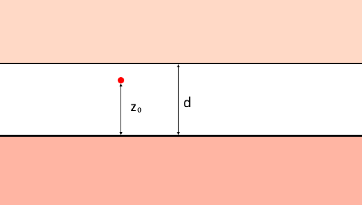
Figure 1: Anisotropic neutral atom between two dielectric half-spaces with plane Chern-Simons boundary layers, $z_{0}$ is a distance of the atom from the layer and the dielectric medium characterized by the index $2$, $d$ is a width of the vacuum slit.

Consider two dielectric half-spaces $z>d$, $z<0$ with dielectric permittivities $\varepsilon_{1}(\omega)$ and $\varepsilon_{2}(\omega)$ respectively and the vacuum slit $0<z<d$ between them. Two Chern-Simons plane parallel boundary layers are located at $z=d$ and $z=0$ and characterized by the parameters $a_{1}(\omega)$ and $a_{2}(\omega)$ respectively (see a discussion after (18)). We omit frequency dispersion in $a_{1}(\omega)$, $a_{2}(\omega)$ for brevity in what follows as before. The atom is located at the point $\mathbf{r^{\prime}}=(0,0,z_{0})$, $0<z_{0}<d$ (see Fig.1). In this Section we derive a general result for the Casimir-Polder potential of a neutral anisotropic atom in this system.

First it is convenient to solve a diffraction problem from an upper half-space ($z\geq d$) when the lower half-space is absent. Consider an upward propagation of an electromagnetic field from a point dipole located at $\mathbf{r^{\prime}}=(0,0,z_{0})$, $z_{0}<d$. For $z<d$ the expansions for electric and magnetic fields can be written as follows:

$$\mathbf{E^{1}}(\omega,\mathbf{r}) =\int\mathbf{N}e^{i\mathbf{k_{\parallel}\cdot r_{\parallel}}}e^{ik_{z}(z-z_{0})}d^{2}\mathbf{k_{\parallel}}+\int\mathbf{v_{1}}e^{i\mathbf{k_{\parallel}\cdot r_{\parallel}}}e^{-ik_{z}z}d^{2}\mathbf{k_{\parallel}}\>,$$ (50)

$$\mathbf{H^{1}}(\omega,\mathbf{r}) =\frac{1}{\omega}\int[\mathbf{k}\times\mathbf{N}]e^{i\mathbf{k_{\parallel}\cdot r_{\parallel}}}e^{ik_{z}(z-z_{0})}d^{2}\mathbf{k_{\parallel}}$$

$$+\frac{1}{\omega}\int\left(\mathbf{[k_{\parallel}\times v_{1}]}-k_{z}\mathbf{[n\times v_{1}]}\right)e^{i\mathbf{k_{\parallel}\cdot r_{\parallel}}}e^{-ik_{z}z}d^{2}\mathbf{k_{\parallel}},$$ (51)

$$\mathbf{N} =\frac{i}{8\pi^{2}k_{z}}\bigl{(}-(\mathbf{k\cdot d})\mathbf{k}+\omega^{2}\mathbf{d}\bigr{)}.$$ (52)

The vector function $\mathbf{v_{1}}$ depends on $\omega,\mathbf{k_{\parallel}}$, $z_{0}$, $d$ and the dipole moment $\mathbf{d}$. For $z>d$ we write transmitted fields in the form

$$\mathbf{E^{2}}(\omega,\mathbf{r}) =\int\mathbf{u_{1}}e^{i\mathbf{k_{\parallel}\cdot r_{\parallel}}}e^{iK_{z1}z}d^{2}\mathbf{k_{\parallel}}\>,$$ (53)

$$\mathbf{H^{2}}(\omega,\mathbf{r}) =\frac{1}{\omega}\int\left(\mathbf{[k_{\parallel}\times u_{1}]}+K_{z1}\mathbf{[n\times u_{1}]}\right)e^{i\mathbf{k_{\parallel}\cdot r_{\parallel}}}e^{iK_{z1}z}d^{2}\mathbf{k_{\parallel}}.$$ (54)

Note that the parameter $a_{1}$ enters boundary conditions

$$H_{x}^{2}|_{z=d+}-H_{x}^{1}|_{z=d-}=2a_{1}E_{x}^{1}|_{z=d},$$ (55)

$$H_{y}^{2}|_{z=d+}-H_{y}^{1}|_{z=d-}=2a_{1}E_{y}^{1}|_{z=d}.$$ (56)

In analogy to Section 2 we find

$$v_{1r} =\biggl{[}-\frac{r_{TM_{1}}+a_{1}^{2}T_{1}}{1+a_{1}^{2}T_{1}}N_{r}+\frac{k_{z}}{\omega}\frac{a_{1}T_{1}}{1+a_{1}^{2}T_{1}}N_{\theta}\biggr{]}e^{ik_{z}(2d-z_{0})},$$ (57)

$$v_{1\theta} =\biggl{[}-\frac{\omega}{k_{z}}\frac{a_{1}T_{1}}{1+a_{1}^{2}T_{1}}N_{r}+\frac{r_{TE_{1}}-a_{1}^{2}T_{1}}{1+a_{1}^{2}T_{1}}N_{\theta}\biggr{]}e^{ik_{z}(2d-z_{0})},$$ (58)

$$v_{1z} =-\frac{k_{r}}{k_{z}}\biggl{[}\frac{r_{TM_{1}}+a_{1}^{2}T_{1}}{1+a_{1}^{2}T_{1}}N_{r}-\frac{k_{z}}{\omega}\frac{a_{1}T_{1}}{1+a_{1}^{2}T_{1}}N_{\theta}\biggr{]}e^{ik_{z}(2d-z_{0})},$$ (59)

where $r_{TM_{1}}$, $r_{TE_{1}}$, $T_{1}$ are written for a medium with a dielectric permittivity $\varepsilon_{1}(\omega)$.

Now we turn to a solution of a diffraction problem when both half-spaces are present. It is convenient to define from (30) the matrices $R_{1}(\omega)$ and $R_{2}(\omega)$ for a reflection of tangential components of the electric field from the media above and below the point dipole respectively in a local basis $\mathbf{e}_{r},\mathbf{e}_{\theta},\mathbf{e}_{z}$:

$$R_{1}(\omega)\equiv R(a_{1},\varepsilon_{1}(\omega),\omega,k_{r}),\>\>R_{2}(\omega)\equiv R(a_{2},\varepsilon_{2}(\omega),\omega,k_{r}),$$ (60)

here the medium for $z\leq 0$ is denoted by the index $2$. Then the tangential local components of the electric field in the interval $0<z<d$ from the point dipole (1),(2) located at $(0,0,z_{0})$ are expressed in terms of matrices $R_{1}(\omega)$, $R_{2}(\omega)$ as follows:

$$\begin{pmatrix}E_{r}\\ E_{\theta}\end{pmatrix}=\frac{e^{ik_{z}z}}{I-R_{2}R_{1}e^{2ik_{z}d}}\biggl{[}R_{2}R_{1}\begin{pmatrix}N_{r}\\ N_{\theta}\end{pmatrix}e^{ik_{z}(2d-z_{0})}+R_{2}\begin{pmatrix}\widetilde{N_{r}}\\ \widetilde{N_{\theta}}\end{pmatrix}e^{ik_{z}z_{0}}\biggr{]}\\ +\frac{e^{ik_{z}(2d-z)}}{I-R_{1}R_{2}e^{2ik_{z}d}}\biggl{[}R_{1}R_{2}\begin{pmatrix}\widetilde{N_{r}}\\ \widetilde{N_{\theta}}\end{pmatrix}e^{ik_{z}z_{0}}+R_{1}\begin{pmatrix}N_{r}\\ N_{\theta}\end{pmatrix}e^{-ik_{z}z_{0}}\biggr{]},$$ (61)

in (61) the local components of the electric field are obtained by a summation of multiple reflections from media with indices $1$ and $2$.

It is convenient to define four matrices entering (61) after Wick rotation:

$$M^{1} =\bigl{(}I-R_{2}(i\omega)R_{1}(i\omega)e^{-2k_{z}d}\bigr{)}^{-1}R_{2}(i\omega)R_{1}(i\omega),$$ (62)

$$M^{2} =\bigl{(}I-R_{2}(i\omega)R_{1}(i\omega)e^{-2k_{z}d}\bigr{)}^{-1}R_{2}(i\omega),$$ (63)

$$M^{3} =\bigl{(}I-R_{1}(i\omega)R_{2}(i\omega)e^{-2k_{z}d}\bigr{)}^{-1}R_{1}(i\omega)R_{2}(i\omega),$$ (64)

$$M^{4} =\bigl{(}I-R_{1}(i\omega)R_{2}(i\omega)e^{-2k_{z}d}\bigr{)}^{-1}R_{1}(i\omega).$$ (65)

Components of scattered electric Green functions can be expressed in terms of matrices (62)-(65) following the scheme explicitly presented in equations (37)-(45). After integration over polar coordinates we express scattered electric Green functions at imaginary frequencies for coinciding arguments $\mathbf{r}=\mathbf{r^{\prime}}$ in terms of matrix elements of matrices (62)-(65):

$$D^{E}_{xx}(i\omega,\mathbf{r}=\mathbf{r^{\prime}})=D^{E}_{yy}(i\omega,\mathbf{r}=\mathbf{r^{\prime}})=-\frac{1}{8\pi}\int\limits_{0}^{\infty}dk_{r}k_{r}\\ \times\biggl{[}k_{z}(e^{-2k_{z}d}M_{11}^{1}+e^{-2k_{z}z_{0}}M_{11}^{2}+e^{-2k_{z}d}M_{11}^{3}+e^{-2k_{z}(d-z_{0})}M_{11}^{4})\\ +\frac{\omega^{2}}{k_{z}}(e^{-2k_{z}d}M_{22}^{1}+e^{-2k_{z}z_{0}}M_{22}^{2}+e^{-2k_{z}d}M_{22}^{3}+e^{-2k_{z}(d-z_{0})}M_{22}^{4})\biggr{]},$$ (66)

$$D^{E}_{zz}(i\omega,\mathbf{r}=\mathbf{r^{\prime}})=-\frac{1}{4\pi}\int\limits_{0}^{\infty}dk_{r}\frac{k_{r}^{3}}{k_{z}}\\ \times\biggl{[}-e^{-2k_{z}d}M_{11}^{1}+e^{-2k_{z}z_{0}}M_{11}^{2}-e^{-2k_{z}d}M_{11}^{3}+e^{-2k_{z}(d-z_{0})}M_{11}^{4})\biggr{]},$$ (67)

$$D^{E}_{xy}(i\omega,\mathbf{r}=\mathbf{r^{\prime}})=-D^{E}_{yx}(i\omega,\mathbf{r}=\mathbf{r^{\prime}})=-\frac{1}{8\pi}\int\limits_{0}^{\infty}dk_{r}k_{r}\\ \times\biggl{[}-\frac{\omega^{2}}{k_{z}}(e^{-2k_{z}d}M_{12}^{1}+e^{-2k_{z}z_{0}}M_{12}^{2}+e^{-2k_{z}d}M_{12}^{3}+e^{-2k_{z}(d-z_{0})}M_{12}^{4})\\ +k_{z}(e^{-2k_{z}d}M_{21}^{1}+e^{-2k_{z}z_{0}}M_{21}^{2}+e^{-2k_{z}d}M_{21}^{3}+e^{-2k_{z}(d-z_{0})}M_{21}^{4})\biggr{]},$$ (68)

$$D^{E}_{xz}(i\omega,\mathbf{r}=\mathbf{r^{\prime}})=D^{E}_{zx}(i\omega,\mathbf{r}=\mathbf{r^{\prime}})=D^{E}_{yz}(i\omega,\mathbf{r}=\mathbf{r^{\prime}})=D^{E}_{zy}(i\omega,\mathbf{r}=\mathbf{r^{\prime}})=0.$$ (69)

Now one can substitute expressions (66)-(69) into the formula (3) and evaluate the Casimir-Polder potential of an anisotropic atom between two dielectric half-spaces with Chern-Simons plane parallel boundary layers. The Casimir-Polder potential in the limit $a_{1}$, $a_{2}\to\infty$ is derived in Appendix A.

IV The Casimir-Polder Potential of an Anisotropic Atom between two Chern-Simons layers in vacuum

In this Section we derive analytic results for the Casimir-Polder potential of an anisotropic atom between two Chern-Simons plane parallel layers in vacuum separated by a distance $d$, the atom is positioned at the point $(0,0,z_{0})$. The layer characterized by the parameter $a_{1}$ is located at $z=d$, the layer characterized by the parameter $a_{2}$ is located at $z=0$.

In the system under consideration $\varepsilon(\omega)=1$ for $z<0$ and $z>d$. In this case the matrices (62)-(65) have the form

$$M^{1}=M^{3}=-\frac{1}{(1+a_{1}^{2})(1+a_{2}^{2})\det[I-R_{1}R_{2}e^{-2k_{z}d}]}\\ \times\begin{pmatrix}a_{1}a_{2}(1-a_{1}a_{2}(1-e^{-2k_{z}d}))&a_{1}a_{2}(a_{1}+a_{2})\frac{k_{z}}{\omega}\\ -a_{1}a_{2}(a_{1}+a_{2})\frac{\omega}{k_{z}}&a_{1}a_{2}(1-a_{1}a_{2}(1-e^{-2k_{z}d}))\end{pmatrix},$$ (70)

$$M^{2}=-\frac{1}{(1+a_{1}^{2})(1+a_{2}^{2})\det[I-R_{1}R_{2}e^{-2k_{z}d}]}\\ \times\begin{pmatrix}a_{2}^{2}(1+a_{1}^{2}(1-e^{-2k_{z}d}))&-a_{2}(1+a_{1}^{2}+a_{1}a_{2}e^{-2k_{z}d})\frac{k_{z}}{\omega}\\ a_{2}(1+a_{1}^{2}+a_{1}a_{2}e^{-2k_{z}d})\frac{\omega}{k_{z}}&a_{2}^{2}(1+a_{1}^{2}(1-e^{-2k_{z}d}))\end{pmatrix},$$ (71)

$$M^{4}=-\frac{1}{(1+a_{1}^{2})(1+a_{2}^{2})\det[I-R_{1}R_{2}e^{-2k_{z}d}]}\\ \times\begin{pmatrix}a_{1}^{2}(1+a_{2}^{2}(1-e^{-2k_{z}d}))&-a_{1}(1+a_{2}^{2}+a_{1}a_{2}e^{-2k_{z}d})\frac{k_{z}}{\omega}\\ a_{1}(1+a_{2}^{2}+a_{1}a_{2}e^{-2k_{z}d})\frac{\omega}{k_{z}}&a_{1}^{2}(1+a_{2}^{2}(1-e^{-2k_{z}d}))\end{pmatrix},$$ (72)

where

$$\frac{1}{(1+a_{1}^{2})(1+a_{2}^{2})\det[I-R_{1}R_{2}e^{-2k_{z}d}]}\\ =\frac{1}{1+a_{1}^{2}+a_{2}^{2}+2a_{1}a_{2}e^{-2k_{z}d}+a_{1}^{2}a_{2}^{2}(1-e^{-2k_{z}d})^{2}}=\frac{\gamma_{1}}{1+\beta_{1}y}+\frac{\gamma_{2}}{1+\beta_{2}y}$$ (73)

with $y=\exp(-2k_{z}d)$, $A=a_{1}^{2}a_{2}^{2}$, $B=2(a_{1}a_{2}-a_{1}^{2}a_{2}^{2})$, $C=(1+a_{1}^{2})(1+a_{2}^{2})$, $y_{1,2}=\frac{-B\pm\sqrt{B^{2}-4AC}}{2A}=(a_{1}a_{2}-1\pm i(a_{1}+a_{2}))/(a_{1}a_{2})$, $\beta_{1}=-1/y_{1}$, $\beta_{2}=-1/y_{2}$, $\gamma_{1}=1/(Ay_{1}(y_{2}-y_{1}))$, $\gamma_{2}=1/(Ay_{2}(y_{1}-y_{2}))$.

Decomposition of the denominator in (73) into two terms leads to an analytic result for the Casimir-Polder potential in terms of Lerch transcendent functions. We change variables

$$\int\limits_{0}^{\infty}k_{r}dk_{r}f(k_{z})=\int\limits_{\omega}^{\infty}k_{z}dk_{z}f(k_{z})$$ (74)

and use the integral

$$G_{0}(\chi,\beta,\omega)\equiv\int\limits_{\omega}^{\infty}\frac{e^{-2k_{z}\chi}}{1+\beta e^{-2k_{z}d}}dk_{z}=\frac{1}{2d}\int\limits_{0}^{e^{-2\omega d}}\frac{y^{\frac{\chi}{d}-1}}{1+\beta y}dy=\frac{e^{-2\omega\chi}}{2d}\Phi\Bigl{(}-\beta e^{-2\omega d},1,\frac{\chi}{d}\Bigr{)},$$ (75)

where $\Phi(\alpha_{1},\alpha_{2},\alpha_{3})$ is a Lerch transcendent function. Derivatives over the parameter $\chi$ are defined as follows:

$$G_{1}(\chi,\beta,\omega)\equiv\frac{1}{2}\frac{d}{d\chi}G_{0}(\chi,\beta,\omega)=-\int\limits_{\omega}^{\infty}k_{z}\frac{e^{-2k_{z}\chi}}{1+\beta e^{-2k_{z}d}}dk_{z},$$ (76)

$$G_{2}(\chi,\beta,\omega)\equiv\frac{1}{4}\frac{d^{2}}{d\chi^{2}}G_{0}(\chi,\beta,\omega)=\int\limits_{\omega}^{\infty}k_{z}^{2}\frac{e^{-2k_{z}\chi}}{1+\beta e^{-2k_{z}d}}dk_{z}.$$ (77)

The Casimir-Polder potential of an anisotropic atom between the two layers is derived by making use of (3), (66)-(68), (70)-(73) and (75)-(77):

$$U_{xx}(z_{0},d)+U_{yy}(z_{0},d)=\frac{1}{16\pi^{2}}\sum\limits_{i=1,2}\gamma_{i}\int\limits_{0}^{\infty}d\omega(\alpha_{xx}(i\omega)+\alpha_{yy}(i\omega))\\ \times\biggl{[}-2a_{1}^{2}a_{2}^{2}G_{2}(2d,\beta_{i},\omega)+2(a_{1}^{2}a_{2}^{2}-a_{1}a_{2})G_{2}(d,\beta_{i},\omega)-a_{2}^{2}(1+a_{1}^{2})G_{2}(z_{0},\beta_{i},\omega)\\ +a_{1}^{2}a_{2}^{2}G_{2}(z_{0}+d,\beta_{i},\omega)-a_{1}^{2}(1+a_{2}^{2})G_{2}(d-z_{0},\beta_{i},\omega)+a_{1}^{2}a_{2}^{2}G_{2}(2d-z_{0},\beta_{i},\omega)\\ +\omega^{2}\biggl{(}-2a_{1}^{2}a_{2}^{2}G_{0}(2d,\beta_{i},\omega)+2(a_{1}^{2}a_{2}^{2}-a_{1}a_{2})G_{0}(d,\beta_{i},\omega)-a_{2}^{2}(1+a_{1}^{2})G_{0}(z_{0},\beta_{i},\omega)\\ +a_{1}^{2}a_{2}^{2}G_{0}(z_{0}+d,\beta_{i},\omega)-a_{1}^{2}(1+a_{2}^{2})G_{0}(d-z_{0},\beta_{i},\omega)+a_{1}^{2}a_{2}^{2}G_{0}(2d-z_{0},\beta_{i},\omega)\biggr{)}\biggr{]},$$ (78)

$$U_{zz}(z_{0},d)=\frac{1}{8\pi^{2}}\sum\limits_{i=1,2}\gamma_{i}\int\limits_{0}^{\infty}d\omega\,\alpha_{zz}(i\omega)\\ \times\biggl{[}2a_{1}^{2}a_{2}^{2}G_{2}(2d,\beta_{i},\omega)-2(a_{1}^{2}a_{2}^{2}-a_{1}a_{2})G_{2}(d,\beta_{i},\omega)-a_{2}^{2}(1+a_{1}^{2})G_{2}(z_{0},\beta_{i},\omega)\\ +a_{1}^{2}a_{2}^{2}G_{2}(z_{0}+d,\beta_{i},\omega)-a_{1}^{2}(1+a_{2}^{2})G_{2}(d-z_{0},\beta_{i},\omega)+a_{1}^{2}a_{2}^{2}G_{2}(2d-z_{0},\beta_{i},\omega)\\ +\omega^{2}\biggl{(}-2a_{1}^{2}a_{2}^{2}G_{0}(2d,\beta_{i},\omega)+2(a_{1}^{2}a_{2}^{2}-a_{1}a_{2})G_{0}(d,\beta_{i},\omega)+a_{2}^{2}(1+a_{1}^{2})G_{0}(z_{0},\beta_{i},\omega)\\ -a_{1}^{2}a_{2}^{2}G_{0}(z_{0}+d,\beta_{i},\omega)+a_{1}^{2}(1+a_{2}^{2})G_{0}(d-z_{0},\beta_{i},\omega)-a_{1}^{2}a_{2}^{2}G_{0}(2d-z_{0},\beta_{i},\omega)\biggr{)}\biggr{]},$$ (79)

$$U_{xy}(z_{0},d)+U_{yx}(z_{0},d)=\frac{1}{8\pi^{2}}\sum\limits_{i=1,2}\gamma_{i}\int\limits_{0}^{\infty}d\omega\,\omega\,(\alpha_{xy}(i\omega)-\alpha_{yx}(i\omega))\\ \times\biggl{[}-2a_{1}a_{2}(a_{1}+a_{2})G_{1}(2d,\beta_{i},\omega)+a_{2}(1+a_{1}^{2})G_{1}(z_{0},\beta_{i},\omega)+a_{1}a_{2}^{2}G_{1}(z_{0}+d,\beta_{i},\omega)\\ +a_{1}(1+a_{2}^{2})G_{1}(d-z_{0},\beta_{i},\omega)+a_{2}a_{1}^{2}G_{1}(2d-z_{0},\beta_{i},\omega)\biggr{]}.$$ (80)

One can express components of the Casimir-Polder potential (78)-(80) in terms of Lerch transcendent functions due to relations

$$G_{1}(\chi,\beta,\omega)=-\frac{e^{-2\omega\chi}}{4d^{2}}\biggl{(}2\omega d\,\Phi\Bigl{(}-\beta e^{-2\omega d},1,\frac{\chi}{d}\Bigr{)}+\Phi\Bigl{(}-\beta e^{-2\omega d},2,\frac{\chi}{d}\Bigr{)}\biggr{)},$$ (81)

$$G_{2}(\chi,\beta,\omega)=\frac{e^{-2\omega\chi}}{4d^{3}}\biggl{(}2\omega^{2}d^{2}\,\Phi\Bigl{(}-\beta e^{-2\omega d},1,\frac{\chi}{d}\Bigr{)}+2\omega d\Phi\Bigl{(}-\beta e^{-2\omega d},2,\frac{\chi}{d}\Bigr{)}\\ +\Phi\Bigl{(}-\beta e^{-2\omega d},3,\frac{\chi}{d}\Bigr{)}\biggr{)}.$$ (82)

At large distances of the atom from the layers $z_{0}$, $d-z_{0}\gg\lambda_{0}\equiv 2\pi/\omega_{0}$, $\lambda_{1}\equiv 2\pi/\omega_{1}$, $\lambda_{2}\equiv 2\pi/\omega_{2}$ ($\lambda_{0}$ is a wavelength corresponding to a typical absorption frequency of the atom $\omega_{0}$, $\lambda_{1}$ and $\lambda_{2}$ are wavelengths of the layers corresponding to absorption frequencies $\omega_{1}$, $\omega_{2}$ of the layers) the Casimir-Polder potential can be derived analytically for arbitrary values of constants $a_{1}$, $a_{2}$ ($a_{1}=a_{1}(0)$ and $a_{2}=a_{2}(0)$ for $z_{0}$, $d-z_{0}\gg\lambda_{1}$, $\lambda_{2}$). Noting that

$$\int\limits_{0}^{\infty}d\omega\,G_{2}(\chi,\beta_{i},\omega)=3\int\limits_{0}^{\infty}d\omega\,\omega^{2}G_{0}(\chi,\beta_{i},\omega)=\frac{3}{8d^{4}}\Phi\Bigl{(}y_{i}^{-1},4,\frac{\chi}{d}\Bigr{)},$$ (83)

we find from (78),(79) the Casimir-Polder potential of the atom between two Chern-Simons plane parallel layers at large distances from the layers resulting from the symmetric part of the atomic polarizability:

$$U_{s}(z_{0},d)=U_{s1}(z_{0},d)+U_{s2}(d)=\frac{\alpha_{xx}(0)+\alpha_{yy}(0)+\alpha_{zz}(0)}{32\pi^{2}d^{4}}\\ \times\sum\limits_{i=1,2}\gamma_{i}\biggl{[}-a_{2}^{2}(1+a_{1}^{2})\Phi\Bigl{(}y_{i}^{-1},4,\frac{z_{0}}{d}\Bigr{)}-a_{1}^{2}(1+a_{2}^{2})\Phi\Bigl{(}y_{i}^{-1},4,\frac{d-z_{0}}{d}\Bigr{)}\\ +a_{1}^{2}a_{2}^{2}\Phi\Bigl{(}y_{i}^{-1},4,\frac{d+z_{0}}{d}\Bigr{)}+a_{1}^{2}a_{2}^{2}\Phi\Bigl{(}y_{i}^{-1},4,\frac{2d-z_{0}}{d}\Bigr{)}\biggr{]}+U_{s2}(d),$$ (84)

$$U_{s2}(d)=\frac{\alpha_{xx}(0)+\alpha_{yy}(0)-\alpha_{zz}(0)}{32\pi^{2}d^{4}}\sum\limits_{i=1,2}{\rm Li}_{4}(y_{i}^{-1})\\ =\frac{\alpha_{xx}(0)+\alpha_{yy}(0)-\alpha_{zz}(0)}{32\pi^{2}d^{4}}\biggl{(}{\rm Li}_{4}\biggl{(}\frac{a_{1}a_{2}}{(a_{1}+i)(a_{2}+i)}\biggr{)}+{\rm Li}_{4}\biggl{(}\frac{a_{1}a_{2}}{(a_{1}-i)(a_{2}-i)}\biggr{)}\biggr{)},$$ (85)

${\rm Li}_{4}(z)$ is a polylogarithm function. For $a_{2}=-a_{1}$ one finds from (84)

$$U_{s}(z_{0},d)=\frac{\alpha_{xx}(0)+\alpha_{yy}(0)+\alpha_{zz}(0)}{32\pi^{2}d^{4}}\\ \times\biggl{[}-\frac{a_{1}^{2}}{1+a_{1}^{2}}\biggl{(}\Phi_{2}\Bigl{(}\frac{a_{1}^{2}}{1+a_{1}^{2}},4,\frac{z_{0}}{d}\Bigr{)}+\Phi_{2}\Bigl{(}\frac{a_{1}^{2}}{1+a_{1}^{2}},4,\frac{d-z_{0}}{d}\Bigr{)}\biggr{)}\\ +\frac{a_{1}^{4}}{(1+a_{1}^{2})^{2}}\biggl{(}\Phi_{2}\Bigl{(}\frac{a_{1}^{2}}{1+a_{1}^{2}},4,\frac{d+z_{0}}{d}\Bigr{)}+\Phi_{2}\Bigl{(}\frac{a_{1}^{2}}{1+a_{1}^{2}},4,\frac{2d-z_{0}}{d}\Bigr{)}\biggr{)}\biggr{]}+U_{s2}(d),$$ (86)

where

$$\Phi_{2}\Bigl{(}z,s,\alpha\Bigr{)}\equiv\Phi\Bigl{(}z,s,\alpha\Bigr{)}+z\frac{\partial\Phi\Bigl{(}z,s,\alpha\Bigr{)}}{\partial z}.$$ (87)

To find the leading contribution to the Casimir-Polder potential at large distances from the layers resulting from the antisymmetric part of the atomic polarizability tensor it is sufficient to take into account the leading term in the expansion of the antisymmetric part of the polarizability tensor for small $\omega$ [50]: $\alpha_{xy}(\omega)-\alpha_{yx}(\omega)\simeq i\omega C_{as}$. In doing so, we obtain from (80) the leading contribution to the Casimir-Polder potential of the atom between two Chern-Simons plane parallel layers at large distances from the layers resulting from the antisymmetric part of the atomic polarizability:

$$U_{as}(z_{0},d)=\frac{C_{as}}{32\pi^{2}d^{5}}\sum\limits_{i=1,2}\gamma_{i}\biggl{[}a_{2}(1+a_{1}^{2})\Phi\Bigl{(}y_{i}^{-1},5,\frac{z_{0}}{d}\Bigr{)}+a_{1}(1+a_{2}^{2})\Phi\Bigl{(}y_{i}^{-1},5,\frac{d-z_{0}}{d}\Bigr{)}\\ +a_{1}a_{2}^{2}\Phi\Bigl{(}y_{i}^{-1},5,\frac{d+z_{0}}{d}\Bigr{)}+a_{2}a_{1}^{2}\Phi\Bigl{(}y_{i}^{-1},5,\frac{2d-z_{0}}{d}\Bigr{)}\biggr{]}+U_{as2}(d),$$ (88)

$$U_{as2}(d)=\frac{C_{as}}{16\pi^{2}d^{5}}\Im\bigl{(}y_{1}{\rm Li}_{5}(y_{1}^{-1})\bigr{)}.$$ (89)

For $a_{2}=-a_{1}$ one finds from (88) and (89)

$$U_{as}(z_{0},d)=\frac{C_{as}}{32\pi^{2}d^{5}}\biggl{[}\frac{a_{1}}{1+a_{1}^{2}}\biggl{(}-\Phi_{2}\Bigl{(}\frac{a_{1}^{2}}{1+a_{1}^{2}},5,\frac{z_{0}}{d}\Bigr{)}+\Phi_{2}\Bigl{(}\frac{a_{1}^{2}}{1+a_{1}^{2}},5,\frac{d-z_{0}}{d}\Bigr{)}\biggr{)}\\ +\frac{a_{1}^{3}}{(1+a_{1}^{2})^{2}}\biggl{(}\Phi_{2}\Bigl{(}\frac{a_{1}^{2}}{1+a_{1}^{2}},5,\frac{d+z_{0}}{d}\Bigr{)}-\Phi_{2}\Bigl{(}\frac{a_{1}^{2}}{1+a_{1}^{2}},5,\frac{2d-z_{0}}{d}\Bigr{)}\biggr{)}\biggr{]}.$$ (90)

In the limit $a_{1}$, $a_{2}\to\infty$ the potential $U_{s}(z_{0},d)$ is in agreement with Barton [70] ($\rho=z_{0}/d$):

$$U_{id}(z_{0},d)=-\frac{\pi^{2}}{96d^{4}} \bigl{(}\alpha_{xx}(0)+\alpha_{yy}(0)+\alpha_{zz}(0)\bigr{)}\frac{3-2\sin^{2}(\pi\rho)}{\sin^{4}(\pi\rho)}$$

$$+\frac{\pi^{2}}{1440d^{4}} \bigl{(}\alpha_{xx}(0)+\alpha_{yy}(0)-\alpha_{zz}(0)\bigr{)},$$ (91)

the asymptotics of $U_{s1}(z_{0},d)$ at large $a_{1}$, $a_{2}$ is derived in Appendix B.

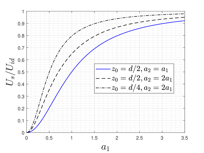
Figure 2: Ratios of the Casimir-Polder potential of a neutral polarizable isotropic atom located between two plane Chern-Simons layers in vacuum $U_{s}(z_{0},d)$ to the potential of the same atom between two perfectly conducting planes $U_{id}(z_{0},d)$, here $z_{0}$ is a distance of the atom from the layer characterized by a constant $a_{2}$, $d$ is a distance between the layers.

We use (84) and (91) to evaluate the ratio of the Casimir-Polder potential of a neutral polarizable atom in the presence of two Chern-Simons plane parallel layers to the Casimir-Polder potential of an atom in the presence of two perfectly conducting parallel planes ($a_{1}\to\infty$, $a_{2}\to\infty$). Ratios $U_{s}/U_{id}$ are shown in Fig.2 for an isotropic atom with $\alpha_{xx}(0)=\alpha_{yy}(0)=\alpha_{zz}(0)$ for $a_{1}=a_{2}$ and $a_{2}=2a_{1}$ in an interval $a_{1}\in[0,3.5]$.

V P-odd vacuum effects

Now we present the most intriguing result of the paper - theoretical prediction of P-odd three-body vacuum effects. By P-odd three-body effects we denote physical effects that differ after $180$ degree rotation of one of the Chern-Simons layers in the presence of a neutral atom. In our notations $180$ degree rotation of one of the layers corresponds to the substitution $a_{1}\to-a_{1}$ (or $a_{2}\to-a_{2}$) into the Casimir-Polder potential. Note that in the model under consideration a neutral polarizable atom interacts via a quantum electrodynamical dipole interaction with an electromagnetic field.

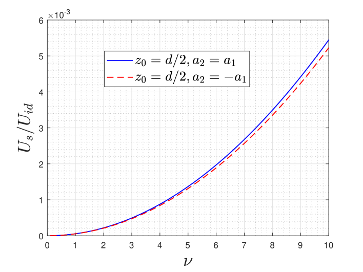
Figure 3: Ratios of the Casimir-Polder potentials $U_{s}(z_{0},d)/U_{id}(z_{0},d)$ differing by $180$ degree rotation of the Chern-Simons layer characterized by a parameter $a_{2}$: $a_{2}=a_{1}$ and $a_{2}=-a_{1}$. Here $z_{0}$ is a distance of the atom from the layer characterized by a constant $a_{2}$, $d$ is a distance between the layers, a dimensionless parameter $\nu=a_{1}/\alpha$ is quantized in quantum Hall layers and Chern insulators.

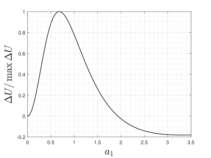
Figure 4: Ratio $\Delta U=U_{s}(z_{0}=d/2,d,a_{2}=-a_{1})-U_{s}(z_{0}=d/2,d,a_{2}=a_{1})$ to $\max\Delta U\approx 0.00587|U_{id}(z_{0}=d/2,d)|$, $\max\Delta U$ holds at $a_{1}\approx 0.678$.

From the formulas (84), (86), (91) we find ratios of potentials $U_{s}(z_{0}=d/2,d,a_{2}=a_{1})$ and $U_{s}(z_{0}=d/2,d,a_{2}=-a_{1})$ to the potential $U_{id}(z_{0}=d/2,d)$ of the atom between two perfectly conducting parallel planes and present these ratios for $\nu=a_{1}/\alpha\leq 10$ in Fig.3. Note that the parameter $\nu$ is quantized in quantum Hall layers and Chern insulators. Values of analogous ratios for larger values of $\nu$ can be extracted from Fig.2 and Fig.4.

In Fig.4 we compare the Casimir-Polder potentials of an isotropic atom for two systems differing by parity of one of the Chern-Simons layers: $a_{2}=a_{1}$ and $a_{2}=-a_{1}$. We use formulas (84), (86) to find ratio of the difference $\Delta U=U_{s}(z_{0}=d/2,d,a_{2}=-a_{1})-U_{s}(z_{0}=d/2,d,a_{2}=a_{1})$ to $\max\Delta U\approx 0.00587|U_{id}(z_{0}=d/2,d)|$, $\max\Delta U$ holds at $a_{1}\approx 0.678$, the ratio is shown in Fig.4. It is interesting to note that the ratio $\max\Delta U/|U_{id}(z_{0}=d/2,d)|\approx 0.00587$ for $a_{1}\approx 0.678$ ($\nu\approx 93$) is even greater than ratios found in Fig.3 for $\nu=10$.

Consider first a classical mechanics reasoning in a gedanken experiment which demonstrates the way to study P-odd effects by neutral atoms in the system of two Chern-Simons plane parallel layers. Consider a neutral atom which starts moving in free space from the point $A$ far away from the layers, continues its movement between the layers so that $z_{0}=d/2$ and finally leaves the space between the layers reaching the point $B$ in free space far away from the layers ($A$, $z_{0}$ and $B$ are on the same straight line parallel to the layers). The Casimir-Polder potential of the atom between two Chern-Simons layers in this case is equal in absolute value to an increase of the kinetic energy of the atom between the layers. The atom moves at a higher speed between the layers than its speed in vacuum, the time difference of the flights with and without Chern-Simons layers can be measured in experiments. When one changes the parameter $a_{1}$ (or $a_{2}$) by changing an external magnetic field in case of a quantum Hall layer or by selecting a layer with a different Chern number in case of a Chern insulator one changes quantum vacuum and the value of the Casimir-Polder potential. At the same time one changes the time of the flight of the atom from the point $A$ to the point $B$. In summary, measuring timeshifts in flight time of neutral atoms through the slit between two Chern-Simons layers is a direct way to study energy shifts in the Casimir-Polder potential due to changes in $a_{1}$, $a_{2}$.

Another possibility to study the Casimir-Polder potential is a measurement of the number of atoms passing through a cavity. The experiment [71] with sodium atoms passing through a micron-sized cavity clearly proved existence of the Casimir-Polder force by measuring the intensity of a sodium atomic beam transmitted through the cavity as a function of separation of cavity boundaries. The experiment [71] can be considered as a prototype of experiments for measurement of P-odd vacuum effects.

One can also study quantum effects of propagation of neutral atoms in a slit between Chern-Simons layers in the presence of a gravitational field. A combined effect of quantum reflection of neutral atoms and the Earth’s gravitational field during propagation of atoms through the slit in analogy to experiments with neutrons [72, 73] should expand experimental capabilities in search of dark matter. Note that quantum reflection of atoms from rigid boundaries arises due to an attractive rapidly changing Casimir-Polder potential [74]. Chern-Simons boundary layers with P-odd vacuum effects lead to new opportunities in this research direction.

VI Conclusions

In this paper we develop a principal generalization of the Green functions scattering method [12] for the case when one can not express the Casimir-Polder potential in terms of diagonal reflection matrix consisting of reflection coefficients for TE and TM modes. Diffraction of an electromagnetic wave in a system with Chern-Simons plane boundary layer is described by a non-diagonal reflection matrix due to rotation of polarizations after reflection of the incoming electromagnetic wave from the layer [37, 38]. The technique developed in this paper is used to derive new formulas for the Casimir-Polder potential of an anisotropic atom in the presence of dielectric half-spaces with Chern-Simons plane parallel boundary layers.

The technique developed in the present paper should be effective for derivation of the Casimir-Polder potential of an anisotropic neutral atom located between any media with plane parallel boundaries when rotation of polarizations occurs after reflection from boundaries. In general, once reflection of electric and magnetic fields from plane parallel boundaries is defined, the Casimir-Polder potential of an anisotropic neutral atom in the system can be found by application of a technique developed in this work.

We have started from derivation of the Casimir-Polder potential of an anisotropic atom in the presence of a dielectric half-space with a Chern-Simons plane layer at its boundary, the result is presented in general formulas (46)-(49). We have continued with derivation of a general result for the Casimir-Polder potential of an anisotropic atom between two dielectric half-spaces with Chern-Simons plane parallel boundary layers, the result is given by expressions (66)-(69) when substituting into a well-known formula (3). This general result is then used to obtain formulas (78)-(80) for the components of the Casimir-Polder potential of an anisotropic atom between two Chern-Simons plane parallel layers in vacuum expressed through Lerch transcendent functions. The Casimir-Polder potential of the atom between two Chern-Simons plane parallel layers at large distances of the atom from both layers is expressed through Lerch transcendent functions and polylogarithms in formulas (84)-(90). All these results for the Casimir-Polder potentials are novel.

Knowledge of formulas for the Casimir-Polder potential of an anisotropic atom between Chern-Simons layers in vacuum and on dielectrics is important for precise comparison of the theory and experiments discussed in Section V. Quantization of parameters $a_{1}$, $a_{2}$ in topological insulators, Chern insulators and quantum Hall layers leads to precise knowledge of the Casimir-Polder potential of the atom at large separations from the boundaries of a cavity with Chern-Simons boundary layers, which is relevant for planning the experiments and conducting precise comparison of the theory and experiments.

Novel P-odd effects for the Casimir-Polder potential between two Chern-Simons plane parallel layers in vacuum due to a substitution $a_{2}\to-a_{2}$ are predicted and analyzed in Section V. P-odd effects arise due to a three-body interaction between a neutral atom in its ground state and two Chern-Simons layers. Our results demonstrate that a neutral atom with QED dipole interaction may become an effective tool for measurement of P-odd vacuum effects due to $180$ degree rotation of one of the Chern-Simons layers. Predicted dependence of the Casimir-Polder potential of a neutral atom on $180$ degree rotation of one of the Chern-Simons layers in a cavity suggests an intriguing fundamental experimental check of quantum vacuum properties based on rotation of the topological material.

Appendix A Perfectly conducting parallel planes

In the limit $a_{1},a_{2}\to\infty$ we find from (30), (62)-(65)

$$M^{1}=M^{3}=-M^{2}=-M^{4}=\frac{1}{1-e^{-2k_{z}d}}\begin{pmatrix}1&0\\ 0&1\end{pmatrix}.$$ (92)

For $a_{1},a_{2}\to\infty$ the Casimir-Polder potential of a neutral atom with a frequency dispersion of the polarizability is derived from (3), (66), (67), (92):

$$U_{2}(z_{0},d)=-\int\limits_{0}^{\infty}\frac{d\omega}{2\pi}\int\limits_{0}^{\infty}\frac{dk_{r}k_{r}}{2\pi}\frac{\exp({-2\sqrt{\omega^{2}+k_{r}^{2}}z_{0}})+\exp({-2\sqrt{\omega^{2}+k_{r}^{2}}(d-z_{0})})}{4\sqrt{\omega^{2}+k_{r}^{2}}(1-\exp({-2\sqrt{\omega^{2}+k_{r}^{2}}d}))}\\ \times\Bigl{[}(2\omega^{2}+k_{r}^{2})\bigl{(}\alpha_{xx}(i\omega)+\alpha_{yy}(i\omega)\bigr{)}+2k_{r}^{2}\alpha_{zz}(i\omega)\Bigr{]}\\ +\int\limits_{0}^{\infty}\frac{d\omega}{2\pi}\int\limits_{0}^{\infty}\frac{dk_{r}k_{r}}{2\pi}\frac{\exp({-2\sqrt{\omega^{2}+k_{r}^{2}}d})}{2\sqrt{\omega^{2}+k_{r}^{2}}(1-\exp({-2\sqrt{\omega^{2}+k_{r}^{2}}d}))}\\ \times\Bigl{[}(2\omega^{2}+k_{r}^{2})\bigl{(}\alpha_{xx}(i\omega)+\alpha_{yy}(i\omega)\bigr{)}-2k_{r}^{2}\alpha_{zz}(i\omega)\Bigr{]}.$$ (93)

The potential $U_{2}(z_{0},d)$ (93) coincides with the Casimir-Polder potential of a neutral anisotropic atom between two perfectly conducting parallel planes [12].

Appendix B Asymptotics

At large distances of the atom from the Chern-Simons layers the Casimir-Polder potential is derived in (84). Now we consider the asymptotics of $U_{s1}(z_{0},d)$ at large $a_{1}$, $a_{2}$.

One can use equality $\gamma_{1}+\gamma_{2}=1/((1+a_{1}^{2})(1+a_{2}^{2}))$ and expansions $y_{1}^{-1}\sim y_{2}^{-1}\sim 1-1/a_{1}^{2}-1/a_{2}^{2}-1/(a_{1}a_{2})$ to write

$$\sum\limits_{i=1,2}\gamma_{i}\Phi(y_{i}^{-1},s,\alpha)=\frac{\Phi(y_{2}^{-1},s,\alpha)}{(1+a_{1}^{2})(1+a_{2}^{2})}+\gamma_{1}\bigl{(}\Phi(y_{1}^{-1},s,\alpha)-\Phi(y_{2}^{-1},s,\alpha)\bigr{)}\\ \approx\frac{\Phi(y_{2}^{-1},s,\alpha)+\Phi^{\prime}(y_{2}^{-1},s,\alpha)y_{1}^{-1}}{(1+a_{1}^{2})(1+a_{2}^{2})}\approx\frac{1}{(1+a_{1}^{2})(1+a_{2}^{2})}\biggl{[}\Phi(1,s,\alpha)+\Phi^{\prime}(1,s,\alpha)\\ -\biggl{(}\frac{1}{a_{1}^{2}}+\frac{1}{a_{2}^{2}}+\frac{1}{a_{1}a_{2}}\biggr{)}\bigl{(}2\Phi^{\prime}(1,s,\alpha)+\Phi^{\prime\prime}(1,s,\alpha)\bigr{)}\biggr{]},$$ (94)

derivatives in Lerch transcendent functions are taken by the first argument. It is convenient to use integral representation of Lerch transcendent function

$$\Phi(z,s,\alpha)=\frac{1}{\Gamma(s)}\int\limits_{0}^{\infty}\frac{t^{s-1}e^{-\alpha t}}{1-ze^{-t}}dt$$ (95)

and expansion (94) to express asymptotics of $U_{s1}(z_{0},d)$ in (84) for large $a_{1}$, $a_{2}$ in terms of Hurwitz zeta function $\zeta(s,\alpha)=\Phi(1,s,\alpha)$ due to integral

$$\int\limits_{0}^{\infty}\frac{t^{s-1}e^{-\alpha t}}{(e^{t}-1)^{2}}dt=\Gamma(s)[\zeta(s-1,\alpha+2)-(\alpha+1)\zeta(s,\alpha+2)]$$ (96)

as follows ($\rho=z_{0}/d$):

$$U_{s1}(z_{0},d)\sim-\frac{\alpha_{xx}(0)+\alpha_{yy}(0)+\alpha_{zz}(0)}{32\pi^{2}d^{4}}\biggl{[}\biggl{(}1-\frac{1}{a_{1}^{2}}-\frac{1}{a_{2}^{2}}\biggr{)}\Bigl{(}\zeta(4,\rho)+\zeta(4,1-\rho)\Bigr{)}\\ +\frac{1}{a_{1}^{2}}\Bigl{(}\zeta(3,\rho)+(1-\rho)\zeta(4,\rho)\Bigr{)}+\frac{1}{a_{2}^{2}}\Bigl{(}\zeta(3,1-\rho)+\rho\,\zeta(4,1-\rho)\Bigr{)}\\ -2\biggl{(}\frac{1}{a_{1}^{2}}+\frac{1}{a_{2}^{2}}+\frac{1}{a_{1}a_{2}}\biggr{)}\Bigl{(}\zeta(3,-\rho+2)+\zeta(3,\rho+1)\\ +(\rho-1)\zeta(4,2-\rho)-\rho\,\zeta(4,\rho+1)\Bigr{)}\biggr{]}.$$ (97)

Note that the asymptotics (97) contains the term proportional to $1/(a_{1}a_{2})$ which changes its sign during 180 degree rotation of one of the Chern-Simons layers ($a_{1}\to-a_{1}$ or $a_{2}\to-a_{2}$). Note also that

$$\zeta(4,\rho)+\zeta(4,1-\rho)=\frac{\pi^{4}}{3}\frac{3-2\sin^{2}(\pi\rho)}{\sin^{4}(\pi\rho)},$$ (98)

so that in the limit $a_{1}\to\infty$, $a_{2}\to\infty$ one gets (91).