An explicit Fourier-Klibanov method for an age-dependent tumor growth model of Gompertz type

Abstract.

This paper proposes an explicit Fourier-Klibanov method as a new approximation technique for an age-dependent population PDE of Gompertz type in modeling the evolution of tumor density in a brain tissue. Through suitable nonlinear and linear transformations, the Gompertz model of interest is transformed into an auxiliary third-order nonlinear PDE. Then, a coupled transport-like PDE system is obtained via an application of the Fourier-Klibanov method, and, thereby, is approximated by the explicit finite difference operators of characteristics. The stability of the resulting difference scheme is analyzed under the standard 2-norm topology. Finally, we present some computational results to demonstrate the effectiveness of the proposed method.

1. Introduction and problem statement

Mathematical modeling is a widely used approach to gain insight into the growth and invasion of cancer cell populations. By leveraging mathematical and computational methods in scientific oncology, researchers can explain various cancer concepts and develop more effective treatment strategies. To investigate the evolutionary dynamics of cancer, several deterministic mathematical models have thus been developed for specific cancer types and stages; see e.g. the monograph [22]. In principle, models of population dynamics are often formulated using a continuum approach based on partial differential equations (PDEs). However, finding analytical solutions to these PDEs is challenging due to the nonlinear structures that account for the complex mechanisms of cancer. Consequently, researchers resort to various approximation methods to obtain numerical solutions to these equations.

In this work, we propose an explicit Fourier-Klibanov method for obtaining numerical solutions to a brain tumor growth model. Tumor growth in population dynamics can be described by various laws (cf. e.g. [18]), including the Von Bertalanffy law that involves

$$f\left(u\right) =\rho u\quad\text{(exponential law)},$$

$$f\left(u\right) =\rho u\left(1-\frac{u}{\mathfrak{C}_{\max}}\right)\quad\text{(Pearl-Verhulst logistic law)},$$

and the Gompertz law,

$$f\left(u\right)=-\rho u\ln\left(\frac{u}{e^{\mathfrak{K}/\text{d}}}\right).$$

We have introduced above various parameters. As to the Von Bertalanffy law, $\rho>0$ denotes the net proliferation rate ($\text{month}^{-1}$), while $\mathfrak{C}_{\max}>0$ represents the maximum number of tumor cells that can occupy a cubic millimeter of brain tissue. For the Gompertz law, the parameter $\mathfrak{K}>0$ describes an exponential increase when $u$ is small, while the damping constant $\text{d}>0$ is to constrain the growth rate when $u$ is large.

Although several studies have focused on approximating tumor growth models using the Von Bertalanffy law (cf. e.g. [19, 6]), there has been limited research specifically dedicated to exploring the Gompertz dynamic. The Gompertzian model is based on the notion that as the tumor size increases, the tumor microenvironment becomes more hostile, and the availability of nutrients and oxygen decreases. Consequently, the tumor’s growth rate decreases, leading to a deceleration in tumor growth. Despite the Gompertzian model’s potential for improving our understanding of tumor dynamics, there is still much to be explored in this area. Further research is needed to fully appreciate the implications of the Gompertzian model in tumor growth dynamics and its potential applications in cancer treatment.

Tumor growth models usually account for variations of tumor in space and time, but their evolution can be further characterized using other parametric variables; see e.g. [21] and references cited therein for the derivation of population models with distinctive parametric arguments. In this study, we focus on the age-dependent process of cell division, where a dividing mother cell gives rise to two daughter cells. By incorporating an aging variable into the above-mentioned Gompertz model, our computational approach is introduced to approximate the following PDE:

(1.1) $$\partial_{t}u+\partial_{a}u-D\left(t,a\right)\partial_{xx}u+\mu\left(a\right)u=-\rho u\ln\left(\frac{u}{e^{\mathfrak{K}/\text{d}}}\right)\quad\text{for }t,a>0,x\in\left(-\ell,\ell\right),$$

where $u=u\left(t,a,x\right)\geq 0$ ($\text{cells (in thousands)}/\text{cm}$) denotes the distribution of the number of tumor cells at time $t$, age $a$ and spatial location $x$. The diffusion of the tumor throughout the brain over time and age is described by the function $D=D\left(t,a\right)$ ($\text{cm}^{2}/\text{month}$) in equation (1.1). Meanwhile, the mortality rate of the population is presented by the age-dependent function $\mu\left(a\right)>0$ ($\text{month}^{-1}$). As we develop our proposed method, we simplify the spatial complexity by considering a one-dimensional model with a length scale of $\ell>0$ (cm). This simplification allows us to focus on the essential features of the tumor growth dynamics and develop a more tractable model for numerical simulations.

To complete the age-dependent Gompertz model, we equip (1.1) with the no-flux boundary condition:

(1.2) $$\partial_{x}u\left(t,a,-\ell\right)=\partial_{x}u\left(t,a,\ell\right)=0\quad\text{for }t,a>0,$$

and the initial data

(1.3) $$u\left(0,a,x\right) =u_{0}\left(a,x\right)\quad\text{for }a>0,x\in\left(-\ell,\ell\right),$$

(1.4) $$u\left(t,0,x\right) =\overline{u}_{0}\left(t,x\right)\quad\text{for }t>0,x\in\left(-\ell,\ell\right).$$

Here, we assume that $u_{0}$ and $\overline{u}_{0}$ satisfy the standard compatibility condition $u_{0}\left(0,\cdot\right)=\overline{u}_{0}\left(0,\cdot\right)$. The zero Neumann boundary condition is commonly imposed to model situations where the tumor is confined to a specific region, such as a tumor in a specific tissue or organ. Furthermore, it is assumed that the functions involved in our PDE system possess sufficient regularity to enable numerical simulation needed for our present purposes. Investigation of the regularity of these functions will be undertaken in forthcoming research.

In many cases, the initial condition for a newborn, denoted by $\overline{u}_{0}$, is accompanied by a nonlocal operator that takes into account the reproductive process, which is weighted by the bounded intrinsic maternity; cf. e.g. [9, 3]. However, this is not the primary focus of our work. Instead, we only examine the regular condition in our Gompertz model. It is worth noting that the nonlocal operator has been successfully linearized through numerical methods in [5]. For every recursive step, the linearization process seeks numerical solutions with the regular newborn boundary condition.

Also, we would like to stress that previous publications have referred to (1.1) as a type of ultra-parabolic equations, with a range of applications beyond the oncological context of this work. For instance, ultra-parabolic PDEs have been found to be crucial in describing heat transfer through a continuous medium in which the presence of the parametric variable $a$ is due to the propagating direction of a shock wave; cf. e.g. [16, 14]. Furthermore, these PDEs have been employed in mathematical finance, specifically for the computation of call option prices. The derivation of the ultra-parabolic PDEs has been detailed in [17], utilizing the ultradiffusion process, wherein the parametric parameter $a$ is determined by the asset price’s path history. It is then worth mentioning that in terms of the ultra-parabolic PDEs, several numerical schemes have been developed for their approximate solution. To name a few, some attempts have been made to design numerical methods for linear equations [1, 2], as well as for nonlinear equations with a globally Lipschitzian source term [7].

Our paper is three-fold. In section 2, we focus on developing an explicit Fourier-Klibanov method for approximating the Gompertz model of interest. The method relies on the derivation of a new coupled nonlinear transport-like PDE system. This can be done by an application of some nonlinear and linear transformations and the special truncated Fourier-Klibanov series. Subsequently, the proposed method is established by applying the explicit finite difference method along with the characteristics of time and age directions. Section 3 is devoted to the $2$-norm stability analysis of the numerical scheme that we have introduced in section 2. Finally, to demonstrate the effectiveness of the proposed method, numerical examples are presented in section 4.

2. Explicit Fourier-Klibanov method

The Fourier-Klibanov method is a technique that utilizes a Fourier series driven by a special orthonormal basis of $L^{2}$. This basis was first constructed in [10], and the Fourier-Klibanov method has since been applied to various physical models of inverse problems. Examples of these models include imaging of land mines, crosswell imaging, and electrical impedance tomography, as demonstrated in recent studies such as [11, 8, 12, 15, 13] and other works cited therein. Thus, our paper is the first to attempt the application of this special basis to approximate a specific class of nonlinear age-dependent population models.

Prior to defining the special basis, several transformations to the PDE (1.1) are employed in the following subsection.

2.1. Derivation of an auxiliary third-order PDE

Let $a_{\dagger}\in\left(0,\infty\right)$ be the maximum age of the cell population in the model. We define the survival probability,

$$\Pi\left(a\right)=e^{-\int_{0}^{a}\mu\left(\sigma\right)d\sigma}.$$

Now, take into account the nonlinear transformation $v=\frac{\ln\left(u/e^{\mathfrak{K}/\text{d}}\right)}{\Pi\left(a\right)}$ or $\frac{u}{e^{\mathfrak{K}/\text{d}}}=e^{\Pi\left(a\right)v}$ for $a\in\left(0,a_{\dagger}\right)$. We compute that

(2.1) $$\partial_{t}u=e^{\mathfrak{K}/\text{d}}\Pi\left(a\right)e^{\Pi\left(a\right)v}\partial_{t}v,\quad\partial_{a}u=e^{\mathfrak{K}/\text{d}}\Pi\left(a\right)e^{\Pi\left(a\right)v}\left(\partial_{a}v-\mu\left(a\right)v\right),\quad\partial_{x}u=e^{\mathfrak{K}/\text{d}}\Pi\left(a\right)e^{\Pi\left(a\right)v}\partial_{x}v,$$

(2.2) $$\partial_{xx}u=e^{\mathfrak{K}/\text{d}}\Pi\left(a\right)\partial_{x}\left(e^{\Pi\left(a\right)v}\partial_{x}v\right)=e^{\mathfrak{K}/\text{d}}\Pi\left(a\right)e^{\Pi\left(a\right)v}\left(\partial_{xx}v+\Pi\left(a\right)\left(\partial_{x}v\right)^{2}\right),$$

(2.3) $$\rho u\ln\left(\frac{u}{e^{\mathfrak{K}/\text{d}}}\right)=\rho e^{\Pi\left(a\right)v}\ln\left(e^{\Pi\left(a\right)v}\right)=\rho e^{\Pi\left(a\right)v}\Pi\left(a\right)v.$$

Combining (2.1)–(2.3), we arrive at the following PDE for $v$:

$$0 =\partial_{t}u+\partial_{a}u-D\left(t,a\right)\partial_{xx}u+\mu\left(a\right)u+\rho u\ln\left(\frac{u}{e^{\mathfrak{K}/\text{d}}}\right)$$

$$=e^{\mathfrak{K}/\text{d}}\Pi\left(a\right)e^{\Pi\left(a\right)v}\left[\partial_{t}v+\partial_{a}v-\mu\left(a\right)v-D\left(t,a\right)\partial_{xx}v\right.$$

$$\left.\hskip 80.00012pt\hskip 40.00006pt\quad-D\left(t,a\right)\Pi\left(a\right)\left(\partial_{x}v\right)^{2}+\mu\left(a\right)\Pi^{-1}\left(a\right)+\rho e^{-\mathfrak{K}/\text{d}}v\right]$$

$$=e^{\mathfrak{K}/\text{d}}\Pi\left(a\right)e^{\Pi\left(a\right)v}\left[\partial_{t}v+\partial_{a}v-D\left(t,a\right)\left(\partial_{xx}v+\Pi\left(a\right)\left(\partial_{x}v\right)^{2}\right)\right.$$

$$\left.\hskip 80.00012pt\hskip 40.00006pt\qquad-\left(\mu\left(a\right)-\rho e^{-\mathfrak{K}/\text{d}}\right)v+\mu\left(a\right)\Pi^{-1}\left(a\right)\right].$$

Vanishing $e^{\mathfrak{K}/\text{d}}\Pi\left(s\right)e^{\Pi\left(s\right)v}$ on the right-hand side of the above equation and then, applying $\partial_{x}$ to the resulting equation, we obtain the following auxiliary PDE:

(2.4) $$\partial_{tx}v+\partial_{ax}v-D\left(t,a\right)\partial_{xxx}v-2D\left(t,a\right)\Pi\left(a\right)\partial_{x}v\partial_{xx}v-\left(\mu\left(a\right)-\rho e^{-\mathfrak{K}/\text{d}}\right)\partial_{x}v=0.$$

2.2. A coupled transport-like system via the Fourier-Klibanov basis

Equation (2.4) is a non-trivial third-order PDE, and we thus propose to apply the Fourier-Klibanov basis $\left\{\Psi_{n}\left(x\right)\right\}_{n=1}^{\infty}$ in $L^{2}\left(-\ell,\ell\right)$ to solve it.

To construct this basis, we start by considering $\varphi_{n}\left(x\right)=x^{n-1}e^{x}$ for $x\in\left[-\ell,\ell\right]$ and $n\in\mathbb{N}$. The set $\left\{\varphi_{n}\left(x\right)\right\}_{n\in\mathbb{N}^{*}}$ is linearly independent and complete in $L^{2}\left(-\ell,\ell\right)$. We then apply the standard Gram-Schmidt orthonormalization procedure to obtain the basis $\left\{\Psi_{n}\left(x\right)\right\}_{n=1}^{\infty}$, which takes the form $P_{n}\left(x\right)e^{x}$, where $P_{n}\left(x\right)$ is the polynomial of the degree $n$.

The Fourier-Klibanov basis possesses the following properties:

• $\Psi_{n}\in C^{\infty}\left[-\ell,\ell\right]$ and $\Psi_{n}^{\prime}\left(x\right)=\Psi_{n}\left(x\right)+P_{n}^{\prime}\left(x\right)e^{x}$ is not identically zero for any $n\in\mathbb{N}^{*}$;

• Let $s_{mn}=\left\langle\Psi_{n}^{\prime},\Psi_{m}\right\rangle$ where $\left\langle\cdot,\cdot\right\rangle$ denotes the scalar product in $L^{2}\left(-\ell,\ell\right)$. Then the square matrix $S_{N}=\left(s_{mn}\right)_{m,n=1}^{N}\in\mathbb{R}^{N\times N}$ is invertible for any $N$ since

$$s_{mn}=\begin{cases}1&\text{if }n=m,\\ 0&\text{if }n<m.\end{cases}$$

Essentially, $S_{N}$ is an upper triangular matrix with $\det\left(S_{N}\right)=1$.

Remark.

The Fourier-Klibanov basis is similar to the orthogonal polynomials formed by the so-called Laguerre functions. However, the Laguerre polynomials are used for the $L^{2}$ basis in the semi-infinite interval with a decaying weighted inner product. We also notice that the second property of the Fourier-Klibanov basis does not hold for either classical orthogonal polynomials or the classical basis of trigonometric functions. The first column of $S_{N}$ obtained from either of the two conventional bases would be zero.

Let $N\geq 1$ now be the cut-off constant. We will discuss how to choose $N$ later in the numerical section. Consider the truncated Fourier series for $v$ in the following sense:

(2.5) $$v\left(t,a,x\right)=\sum_{n=1}^{N}\left\langle v\left(t,a,\cdot\right),\Psi_{n}\left(\cdot\right)\right\rangle\Psi_{n}\left(x\right)=\sum_{n=1}^{N}v_{n}\left(t,a\right)\Psi_{n}\left(x\right).$$

Plugging this truncated series into the auxiliary PDE (2.4), we have

(2.6) $$\sum_{n=1}^{N}\left[\left(\partial_{t}+\partial_{a}\right)-\left(\mu\left(a\right)-\rho e^{-\mathfrak{K}/\text{d}}\right)\right]v_{n}\left(t,a\right)\Psi_{n}^{\prime}\left(x\right)$$

$$=D\left(t,a\right)\sum_{n=1}^{N}v_{n}\left(t,a\right)\Psi_{n}^{\prime\prime\prime}\left(x\right)+2D\left(t,a\right)\Pi\left(a\right)\sum_{n=1}^{N}\sum_{k=1}^{N}v_{n}\left(t,a\right)v_{k}\left(t,a\right)\Psi_{n}^{\prime}\left(x\right)\Psi_{k}^{\prime\prime}\left(x\right).$$

For each $1\leq m\leq N$, we multiply both sides of (2.6) by $\Psi_{m}$ and then integrate both sides of the resulting equation from $x=-\ell$ to $x=\ell$. Let $V=\left(v_{1},v_{1},...,v_{N}\right)^{\text{T}}\in\mathbb{R}^{N}$ be the $N$-dimensional vector-valued function that contains all of the Fourier coefficients $v_{n}$. We obtain the following nonlinear PDE system:

(2.7) $$\sum_{n=1}^{N}s_{mn} \left[\left(\partial_{t}+\partial_{a}\right)-\left(\mu\left(a\right)-\rho e^{-\mathfrak{K}/\text{d}}\right)\right]v_{n}\left(t,a\right)$$

$$=D\left(t,a\right)\sum_{n=1}^{N}\kappa_{mn}v_{n}\left(t,a\right)+2D\left(t,a\right)\Pi\left(a\right)\sum_{n=1}^{N}\sum_{k=1}^{N}\varsigma_{mnk}v_{n}\left(t,a\right)v_{k}\left(t,a\right),$$

where $\kappa_{mn}=\left\langle\Psi_{n}^{\prime\prime\prime},\Psi_{m}\right\rangle$ and $\varsigma_{mnk}=\left\langle\Psi_{n}^{\prime}\Psi_{k}^{\prime\prime},\Psi_{m}\right\rangle$. It is straightforward to see that system (2.7) is of the transport-like form. By the boundary data (1.3) and (1.4), we associate (2.7) with the following boundary conditions:

(2.8) $$v_{n}\left(0,a\right) =\left\langle v\left(0,a,\cdot\right),\Psi_{n}\left(\cdot\right)\right\rangle=\Pi^{-1}\left(a\right)\left\langle\ln\left(u_{0}\left(a,\cdot\right)/e^{\mathfrak{K}/\text{d}}\right),\Psi_{n}\left(\cdot\right)\right\rangle,$$

(2.9) $$v_{n}\left(t,0\right) =\left\langle v\left(t,0,\cdot\right),\Psi_{n}\left(\cdot\right)\right\rangle=\left\langle\ln\left(\overline{u}_{0}\left(t,\cdot\right)/e^{\mathfrak{K}/\text{d}}\right),\Psi_{n}\left(\cdot\right)\right\rangle.$$

2.3. Finite difference operators

To approximate the transport-like system (2.7)–(2.9), we propose to apply the so-called finite difference method of characteristics in the time-age direction. To do so, we take into account the time increment $\Delta t=T/M$ for $M\geq 2$ being a fixed integer. Then, we set the mesh-point in time by $t_{i}=i\Delta t$ for $0\leq i\leq M$. Using the number $M$, we define $K=\left[a_{\dagger}/\Delta t+1\right]$ and set the mesh-point in age by

$$a_{j}=j\Delta t\quad\text{for }0\leq j<K.$$

Thus, we discretize the differential operator $\partial_{t}+\partial_{a}$ along the characteristic $t=a$, as follows:

$$\left(\partial_{t}+\partial_{a}\right)v_{n}\left(t_{i},a_{j}\right)=\frac{v_{n,j}^{i}-v_{n,j}^{i-1}}{\Delta t}+\frac{v_{n,j}^{i-1}-v_{n,j-1}^{i-1}}{\Delta t}=\frac{v_{n,j}^{i}-v_{n,j-1}^{i-1}}{\Delta t}.$$

Here and to this end, the subscript $j$ indicates the age level $a_{j}$ and the superscript $i$ implies the time level $t_{i}$. By the forward Euler procedure, we then seek the discrete solution $v_{n,j}^{i}=v_{n}\left(t_{i},a_{j}\right)$ of the following systematic scheme:

$$\sum_{n=0}^{N-1}s_{mn}v_{n,j}^{i} =\sum_{n=0}^{N-1}s_{mn}v_{n,j-1}^{i-1}+\Delta t\sum_{n=0}^{N-1}\left[s_{mn}\left(\mu_{j-1}-\rho e^{-\mathfrak{K}/\text{d}}\right)+D_{j-1}^{i-1}\kappa_{mn}\right]v_{n,j-1}^{i-1}$$

$$+2\Delta tD_{j-1}^{i-1}\Pi_{j-1}\sum_{n=0}^{N-1}\sum_{k=0}^{N-1}\varsigma_{mnk}v_{n,j-1}^{i-1}v_{k,j-1}^{i-1}$$

for $i,j\geq 1$. Now, for every step $\left(i,j\right)$, let $\mathbb{K}_{j}^{i}=\left(\mathbb{K}_{mn,j}^{i}\right)_{m,n=1}^{N}$ with $\mathbb{K}_{mn,j}^{i}=s_{mn}\left(\mu_{j}-\rho e^{-\mathfrak{K}/\text{d}}\right)+D_{j}^{i}\kappa_{mn}$ and let $\mathbb{G}_{m,j}^{i}=\left(\mathbb{G}_{mnk,j}^{i}\right)_{n,k=1}^{N}$ with $\mathbb{G}_{mnk,j}^{i}=2D_{j}^{i}\Pi_{j}\varsigma_{mnk}$. Henceforth, our discretized coupled system has the following form:

(2.10) $$S_{N}V_{j}^{i}=S_{N}V_{j-1}^{i-1}+\Delta t\mathbb{K}_{j-1}^{i-1}V_{j-1}^{i-1}+\Delta t\begin{bmatrix}\left(V_{j-1}^{i-1}\right)^{\text{T}}\mathbb{G}_{1,j-1}^{i-1}V_{j-1}^{i-1}\\ \left(V_{j-1}^{i-1}\right)^{\text{T}}\mathbb{G}_{2,j-1}^{i-1}V_{j-1}^{i-1}\\ \left(V_{j-1}^{i-1}\right)^{\text{T}}\mathbb{G}_{3,j-1}^{i-1}V_{j-1}^{i-1}\\ \vdots\\ \left(V_{j-1}^{i-1}\right)^{\text{T}}\mathbb{G}_{N,j-1}^{i-1}V_{j-1}^{i-1}\end{bmatrix}.$$

By (2.8) and (2.9), this system is associated with the starting points $V_{j}^{0}=\left(v_{n}\left(0,a_{j}\right)\right)_{n=1}^{N}$ and $V_{0}^{i}=\left(v_{n}\left(t_{i},0\right)\right)_{n=1}^{N}$.

3. Stability analysis

In this section, we want to analyze the stability of the proposed explicit approach. Before doing so, we want to ensure that the discrete solution $V_{j}^{i}$ is uniformly bounded for any bounded data $V_{j}^{0}$ and $V_{0}^{i}$. To this end, we make use of the following $2$-norm of any vector $X=\left(X_{n}\right)_{n=1}^{N}\in\mathbb{R}^{N}$.

(3.1) $$\left|X\right|_{2}=\left(\sum_{1\leq n\leq N}\left|X_{n}\right|^{2}\right)^{1/2}.$$

Also, for any square matrix $X=\left(X_{mn}\right)_{m,n=1}^{N}\in\mathbb{R}^{N\times N}$, we use the Frobenius norm,

(3.2) $$\left|X\right|_{F}=\left(\sum_{m=1}^{N}\sum_{n=1}^{N}\left|X_{mn}\right|^{2}\right)^{1/2}.$$

It follows from (2.10) that for $i,j\geq 1$,

(3.3) $$S_{N}V_{j}^{i}=\begin{cases}S_{N}V_{0}^{i-j}+\Delta t\sum_{\mathfrak{i}=0}^{j-1}\mathbb{F}\left(V_{\mathfrak{i}}^{\mathfrak{i}+i-j}\right),&\text{if }i\geq j,\\ S_{N}V_{j-i}^{0}+\Delta t\sum_{\mathfrak{j}=0}^{i-1}\mathbb{F}\left(V_{\mathfrak{j}+j-i}^{\mathfrak{j}}\right),&\text{if }i<j,\end{cases}$$

where the nonlinear term $\mathbb{F}:\mathbb{R}^{N}\to\mathbb{R}^{N}$ is defined as

$$\mathbb{F}\left(V_{\mathfrak{j}}^{\mathfrak{i}}\right)=\mathbb{K}_{\mathfrak{j}}^{\mathfrak{i}}V_{\mathfrak{j}}^{\mathfrak{i}}+\begin{bmatrix}\left(V_{\mathfrak{j}}^{\mathfrak{i}}\right)^{\text{T}}\mathbb{G}_{1,\mathfrak{j}}^{\mathfrak{i}}V_{\mathfrak{j}}^{\mathfrak{i}}\\ \left(V_{\mathfrak{j}}^{\mathfrak{i}}\right)^{\text{T}}\mathbb{G}_{2,\mathfrak{j}}^{\mathfrak{i}}V_{\mathfrak{j}}^{\mathfrak{i}}\\ \left(V_{\mathfrak{j}}^{\mathfrak{i}}\right)^{\text{T}}\mathbb{G}_{3,\mathfrak{j}}^{\mathfrak{i}}V_{\mathfrak{j}}^{\mathfrak{i}}\\ \vdots\\ \left(V_{\mathfrak{j}}^{\mathfrak{i}}\right)^{\text{T}}\mathbb{G}_{N,\mathfrak{j}}^{\mathfrak{i}}V_{\mathfrak{j}}^{\mathfrak{i}}\end{bmatrix}.$$

Let $S_{N}^{-1}=\left(\tilde{s}_{mn}\right)_{m,n=1}^{N}\in\mathbb{R}^{N\times N}$ be the inverse of $S_{N}$. We can rewrite (3.3) as

(3.4) $$V_{j}^{i}=\begin{cases}V_{0}^{i-j}+\Delta tS_{N}^{-1}\sum_{\mathfrak{i}=0}^{j-1}\mathbb{F}\left(V_{\mathfrak{i}}^{\mathfrak{i}+i-j}\right),&\text{if }i\geq j,\\ V_{j-i}^{0}+\Delta tS_{N}^{-1}\sum_{\mathfrak{j}=0}^{i-1}\mathbb{F}\left(V_{\mathfrak{j}+j-i}^{\mathfrak{j}}\right),&\text{if }i<j.\end{cases}$$

Theorem 1.

Assume that there exists a constant $C>0$ independent of $i$ and $j$ such that

(3.5) $$\max_{j\geq 0}\left|V_{j}^{0}\right|_{2}\leq C,\quad\text{and }\max_{i\geq 0}\left|V_{i}^{0}\right|_{2}\leq C.$$

Moreover, suppose that for each $i,j\geq 0$, we can find a constant $P_{j}^{i}\geq 0$ such that

(3.6) $$\left|\mathbb{K}_{j}^{i}\right|_{F}+\sum_{m=1}^{N}\left|\mathbb{G}_{m,\mathfrak{j}}^{\mathfrak{i}}\right|_{F}\leq P_{j}^{i}.$$

Then for any time step $\Delta t$ sufficiently small with

(3.7) $$\Delta t\left|S_{N}^{-1}\right|_{F}\sum_{i,j\geq 0}P_{j}^{i}\leq\ln\left(\frac{C+1}{C+\frac{1}{2}}\right),$$

the discrete solution $V_{j}^{i}$ in (3.3) is bounded by

(3.8) $$\max_{i,j\geq 0}\left|V_{j}^{i}\right|_{2}\leq 2C.$$

Proof.

It is straightforward to see that

$$\left|\mathbb{F}\left(V_{\mathfrak{j}}^{\mathfrak{i}}\right)\right|_{2} \leq\left|\mathbb{K}_{\mathfrak{j}}^{\mathfrak{i}}V_{\mathfrak{j}}^{\mathfrak{i}}\right|_{2}+\left|\left(V_{\mathfrak{j}}^{\mathfrak{i}}\right)^{\text{T}}\mathbb{G}_{\mathfrak{j}}^{\mathfrak{i}}V_{\mathfrak{j}}^{\mathfrak{i}}\right|_{2}$$

$$\leq\left|\mathbb{K}_{\mathfrak{j}}^{\mathfrak{i}}\right|_{F}\left|V_{\mathfrak{j}}^{\mathfrak{i}}\right|_{2}+\sum_{m=1}^{N}\left|\mathbb{G}_{m,\mathfrak{j}}^{\mathfrak{i}}\right|_{F}\left|V_{\mathfrak{j}}^{\mathfrak{i}}\right|_{2}^{2}.$$

Therefore, by (3.6) and (3.4), we estimate that for $i\geq j$,

$$\left|V_{j}^{i}\right|_{2} \leq\left|V_{0}^{i-j}\right|_{2}+\Delta t\left|S_{N}^{-1}\right|_{F}\sum_{\mathfrak{i}=0}^{j-1}\left|\mathbb{F}\left(V_{\mathfrak{i}}^{\mathfrak{i}+i-j}\right)\right|_{2}$$

(3.9) $$\leq C+\Delta t\left|S_{N}^{-1}\right|_{F}\sum_{\mathfrak{i}=0}^{j-1}P_{\mathfrak{i}}^{\mathfrak{i}+i-j}\left(\left|V_{\mathfrak{i}}^{\mathfrak{i}+i-j}\right|_{2}+\left|V_{\mathfrak{i}}^{\mathfrak{i}+i-j}\right|_{2}^{2}\right).$$

Now, with the aid of the discrete Gronwall-Bellman-Ou-Iang inequality (cf. [4, Theorem 2.1]) applied to (3.9), we deduce that

(3.10) $$\left|V_{j}^{i}\right|_{2}\leq\Phi^{-1}\left[\Phi\left(C\right)+\Delta t\left|S_{N}^{-1}\right|_{F}\sum_{\mathfrak{i}=0}^{i-1}\sum_{\mathfrak{j}=0}^{j-1}P_{\mathfrak{j}}^{\mathfrak{i}}\right],$$

where $\Phi^{-1}$ is the inverse of $\Phi$, and $\Phi$ is given by

$$\Phi\left(f\right)=\int_{1}^{f}\frac{dr}{r+r^{2}}=\ln\left(\frac{2f}{f+1}\right)\quad\text{for }f>0.$$

Herewith, the denominator is obtained from the structure of the second component on the right-hand side of the bound (3.9). With this structure in mind, we can find $\Phi^{-1}$ as follows:

$$\Phi^{-1}\left(f\right)=\frac{e^{f}}{2-e^{f}}=\frac{1}{2e^{-f}-1}\quad\text{for }f\in\left(0,\ln 2\right).$$

Next, by our choice in (3.7), we mean that

$$\left(C+1\right)\exp\left(-\Delta t\left|S_{N}^{-1}\right|_{F}\sum_{\mathfrak{i}=0}^{i-1}\sum_{\mathfrak{j}=0}^{j-1}P_{\mathfrak{j}}^{\mathfrak{i}}\right)\geq C+\frac{1}{2}>C,$$

Henceforth, for $i\geq j$, it follows from (3.10) that

$$\left|V_{j}^{i}\right|_{2} \leq\left[2\exp\left(-\Phi\left(C\right)-\Delta t\left|S_{N}^{-1}\right|_{F}\sum_{\mathfrak{i}=0}^{i-1}\sum_{\mathfrak{j}=0}^{j-1}P_{\mathfrak{j}}^{\mathfrak{i}}\right)-1\right]^{-1}$$

$$=\left[2\exp\left(-\ln\left(\frac{2C}{C+1}\right)-\Delta t\left|S_{N}^{-1}\right|_{F}\sum_{\mathfrak{i}=0}^{i-1}\sum_{\mathfrak{j}=0}^{j-1}P_{\mathfrak{j}}^{\mathfrak{i}}\right)-1\right]^{-1}$$

$$=\left[\frac{C+1}{C}\exp\left(-\Delta t\left|S_{N}^{-1}\right|_{F}\sum_{\mathfrak{i}=0}^{i-1}\sum_{\mathfrak{j}=0}^{j-1}P_{\mathfrak{j}}^{\mathfrak{i}}\right)-1\right]^{-1}.$$

which allows us to obtain the target estimate (3.8) for $i\geq j$. Using the same argument, we also have (3.8) for $i<j$ by means of the following estimate:

$$\left|V_{j}^{i}\right|_{2}\leq C+\Delta t\left|S_{N}^{-1}\right|_{F}\sum_{\mathfrak{j}=0}^{i-1}P_{\mathfrak{j}+j-i}^{\mathfrak{j}}\left(\left|V_{\mathfrak{j}+j-i}^{\mathfrak{j}}\right|_{2}+\left|V_{\mathfrak{j}+j-i}^{\mathfrak{j}}\right|_{2}^{2}\right)\quad\text{for }i<j.$$

Hence, we complete the proof of the theorem. ∎

Theorem 1 implies that for any $i,j\geq 1$, the discrete solution $V_{j}^{i}$ of the numerical scheme and its initial data stay in the same ball $\mathcal{B}\left(0,2C\right)$ under the topology of the $2$-norm. This essence allows us to analyze the stability of the proposed scheme (3.3). Let $W_{j}^{i}=V_{j}^{i}-\tilde{V}_{j}^{i}$, where $V_{j}^{i}$ and $\tilde{V}_{j}^{i}$ satisfy 3.4 corresponding to the initial data $\left(V_{j}^{0},V_{0}^{i}\right)$ and $\left(\tilde{V}_{j}^{0},\tilde{V}_{0}^{i}\right)$, respectively. Our stability analysis is formulated in the following theorem.

Theorem 2.

Under the assumptions of Theorem 1, we can show that for all $i,j\geq 0$, the following estimate holds true:

$$\left|W_{j}^{i}\right|_{2}\leq\left(\left|W_{0}^{i-j}\right|_{2}+\left|W_{j-i}^{0}\right|_{2}\right)\left[1+\left(1+4C\right)\ln\left(\frac{C+1}{C+\frac{1}{2}}\right)\right].$$

Proof.

From 3.4,we can compute that for $i\geq j$,

(3.11) $$W_{j}^{i}=W_{0}^{i-j}+\Delta tS_{N}^{-1}\sum_{\mathfrak{i}=0}^{j-1}\left[\mathbb{F}\left(V_{\mathfrak{i}}^{\mathfrak{i}+i-j}\right)-\mathbb{F}\left(\tilde{V}_{\mathfrak{i}}^{\mathfrak{i}+i-j}\right)\right].$$

In view of the fact that

$$V^{T}G_{m}V-\tilde{V}^{T}G_{m}\tilde{V} =V^{T}\left(G_{m}V-G_{m}\tilde{V}\right)+\left(V^{T}-\tilde{V}^{T}\right)G_{m}\tilde{V}$$

$$=V^{T}G_{m}\left(V-\tilde{V}\right)+\left(V^{T}-\tilde{V}^{T}\right)G_{m}\tilde{V},$$

we, in conjunction with (3.6) and (3.8), have

$$\left|\mathbb{F}\left(V_{\mathfrak{j}}^{\mathfrak{i}}\right)-\mathbb{F}\left(\tilde{V}_{\mathfrak{j}}^{\mathfrak{i}}\right)\right|_{2} \leq\left|\mathbb{K}_{\mathfrak{j}}^{\mathfrak{i}}\right|_{F}\left|W_{\mathfrak{j}}^{\mathfrak{i}}\right|_{2}+\sum_{m=1}^{N}\left|\mathbb{G}_{m,\mathfrak{j}}^{\mathfrak{i}}\right|_{F}\left(\left|V_{\mathfrak{j}}^{\mathfrak{i}}\right|_{2}+\left|\tilde{V}_{\mathfrak{j}}^{\mathfrak{i}}\right|_{2}\right)\left|W_{\mathfrak{j}}^{\mathfrak{i}}\right|_{2}$$

$$\leq P_{j}^{i}\left(1+4C\right)\left|W_{\mathfrak{j}}^{\mathfrak{i}}\right|_{2}.$$

Therefore, applying to the $2$-norm to (3.11), we estimate that

$$\left|W_{j}^{i}\right|_{2} \leq\left|W_{0}^{i-j}\right|_{2}+\Delta t\left|S_{N}^{-1}\right|_{F}\sum_{\mathfrak{i}=0}^{j-1}\left|\mathbb{F}\left(V_{\mathfrak{i}}^{\mathfrak{i}+i-j}\right)-\mathbb{F}\left(\tilde{V}_{\mathfrak{i}}^{\mathfrak{i}+i-j}\right)\right|_{2}$$

$$\leq\left|W_{0}^{i-j}\right|_{2}+\Delta t\left|S_{N}^{-1}\right|_{F}\sum_{\mathfrak{i}=0}^{j-1}P_{j}^{i}\left(1+4C\right)\left|W_{\mathfrak{j}}^{\mathfrak{i}}\right|_{2}.$$

Using the Salem-Raslan inequality (cf. [20, Theorem 6.1.3]), we thus obtain that for $i\geq j$,

$$\left|W_{j}^{i}\right|_{2}\leq\left|W_{0}^{i-j}\right|_{2}\left[1+\Delta t\left|S_{N}^{-1}\right|_{F}\left(1+4C\right)\sum_{\mathfrak{i}=0}^{j-1}P_{j}^{i}\right]\leq\left|W_{0}^{i-j}\right|_{2}\left[1+\left(1+4C\right)\ln\left(\frac{C+1}{C+\frac{1}{2}}\right)\right].$$

For $i<j$, we can follow the same procedure to get

$$\left|W_{j}^{i}\right|_{2}\leq\left|W_{j-i}^{0}\right|_{2}\left[1+\left(1+4C\right)\ln\left(\frac{C+1}{C+\frac{1}{2}}\right)\right].$$

Hence, we complete the proof of the theorem. ∎

4. Numerical results

In this section, we want to verify the numerical performance of the proposed explicit Fourier-Klibanov method. By the inception of the method, comparing it with the other numerical methods is not within the scope of this paper. In fact, from our best knowledge, there appears to be no numerical schemes studied for the age-dependent population diffusion model of Gompertz type.

In our population model of interest, the mortality function is often chosen as $\mu\left(a\right)=\left(a_{\dagger}-a\right)^{-1}$, which is unbounded at $a=a_{\dagger}$. We will use this function in all numerical experiments. Furthermore, for this particular choice, the survival probability can be computed explicitly,

$$\Pi\left(a\right)=e^{-\int_{0}^{a}\mu\left(\sigma\right)d\sigma}=\frac{a_{\dagger}-a}{a_{\dagger}},\quad\text{and }\Pi\left(a_{\dagger}\right)=0.$$

Besides, we fix $\ell=1$ and $\Delta x=0.05$ , indicating that we are looking at the dynamics of tumor cells within a length scale of 2 (cm) and a step-size of $0.5$ (mm). We also fix $T=10$ (months) and examine the model with the maximum age of $a_{\dagger}=12$ (months). Besides, $\mathfrak{K}=\text{d}=1$ are dimensionless and fixed.

Remark 3.

The population dynamics of cancer typically involve determining the total population of tumor cells within specific age and spatial ranges. This information is crucial in understanding the local/global burden of cancer in the body, including the size and extent of the tumor. In our numerical experiments, we consider

$$p\left(t\right)=\int_{-\ell}^{\ell}\int_{0}^{a_{\dagger}}u\left(t,a,x\right)dadx$$

as the (global) total population in time. In addition to ensuring numerical stability of the density $u\left(t,a,x\right)$, we also place importance on the stability of the total population, as it allows us to obtain a macroscopic perspective of the entire simulation. To approximate the time-dependent two-dimensional function $p\left(t\right)$ based on discrete approximations of $u\left(t,a,x\right)$ (via the proposed explicit Fourier-Klibanov scheme), we use the standard trapezoidal rule. It is worth noting that, as mentioned above, we have fixed the following parameters: $\ell=1,a_{\dagger}=12$ and $\Delta x=0.05$, while $\Delta a$ varies depending on the chosen value of $M$.

4.1. Choice of the cut-off constant

We discuss how we determine the cut-off constant $N$ for the truncated Fourier-Klibanov series. For each example, we explicitly select the initial data $u_{0}\left(a,x\right)$, which we use to calculate $v_{0}\left(a,x\right)$ through the nonlinear transformation $v=\frac{\ln\left(u/e^{\mathfrak{K}/\text{d}}\right)}{\Pi\left(a\right)}$. Denote the resulting transformed initial data as $v_{0}^{\text{true}}\left(a,x\right)$ and its corresponding approximation as $v_{0,N}^{\text{true}}\left(a,x\right)$. With the explicit form of $v_{0}^{\text{true}}\left(a,x\right)$ and the basis $\left\{\Psi_{n}\left(x\right)\right\}_{n=1}^{\infty}$, we can plug them into the truncated series (2.5) to compute $v_{0,N}^{\text{true}}\left(a,x\right)$. This allows us to compute the following relative max error:

$$E_{\max}\left(v_{0}^{\text{true}},v_{0,N}^{\text{true}}\right)=\frac{\max_{j,l\geq 0}\left|v_{0}^{\text{true}}\left(a_{j},x_{l}\right)-v_{0,N}^{\text{true}}\left(a_{j},x_{l}\right)\right|}{\max_{j,l\geq 0}\left|v_{0}^{\text{true}}\left(a_{j},x_{l}\right)\right|}\times 100\%.$$

For convenience, we set the age step to 40, ensuring consistency with the number of nodes in the space variable. It should be noted that $\Delta x=0.05$, $\ell=1$ and $a_{\dagger}=12$ remain fixed in seeking $N$.

Cf. Table 1, we can see that the relative max error, $E_{\max}\left(v_{0}^{\text{true}},v_{0,N}^{\text{true}}\right)$, decreases rapidly as $N$ increases. In Example 1, increasing $N$ from 2 to 4 results in a reduction of $E_{\max}$ by a factor of approximately 30, while it is 10 in Examples 2 and 3. To better address how well the truncated Fourier-Klibanov works, we present in Figure 4.1 graphical representations of $v_{0}^{\text{true}}$ and $v_{0,N}^{\text{true}}$ for $N=2$ and $N=6$ for all examples.

Observe the first row of Figure 4.1, which represents the approximation by the truncated series for Example 1. When $N=2$, the approximation is not good in terms of two criteria: the maximum absolute value and the shape of the graph. However, when $N=6$, the approximation fulfills both criteria very well.

The second row of Figure 4.1 shows the same performance for Example 2. Since the Fourier-Klibanov series $v_{0,N}^{\text{true}}$ approximates $v_{0}^{\text{true}}$ so well in this example, we deliberately present the log scale for the value of such $v_{0}^{\text{true}}$ and $v_{0,N}^{\text{true}}$ to show the convergence. Without the log scale, it is difficult to see the significant improvement of the series in terms of the two criteria when increasing $N$ from 2 to 6.

The last row of Figure 4.1 also demonstrates the same performance. When $N=2$, $v_{0}^{\text{true}}$ and $v_{0,N}^{\text{true}}$ have the same shape, yielding a relatively good accuracy of the series. When $N$ is increased to 6, the value of $v_{0,N}^{\text{true}}$ is very close to $v_{0}^{\text{true}}$.

It is noteworthy that the maximum absolute value of $v_{0}^{\text{true}}$ in all examples is very large. However, despite this, the truncated Fourier-Klibanov series demonstrates high accuracy in the relative maximum error. Overall, the graphical representation shows that the approximation for $N=6$ is in complete agreement with the true value, confirming the accuracy we have analyzed. Based on these numerical observations, we choose $N=6$ for all subsequent experiments.

Example	$N$	$E_{\max}$	Example	$N$	$E_{\max}$	Example	$N$	$E_{\max}$
1	2	29.35%	2	2	61.68%	3	2	61.33%
	4	0.972%		4	6.746%		4	5.951%
	6	0.012%		6	0.160%		6	0.134%

Table 1. The relative max error $E_{\max}\left(v_{0}^{\text{true}},v_{0,N}^{\text{true}}\right)$ decreases when $N$ becomes large. This is observed while keeping the mesh grid of space and age fixed with $\Delta x=\Delta t=0.05$. By these numerical observations, taking $N=6$ is acceptable for all numerical experiments in the sense that the relative max error is sufficiently small.

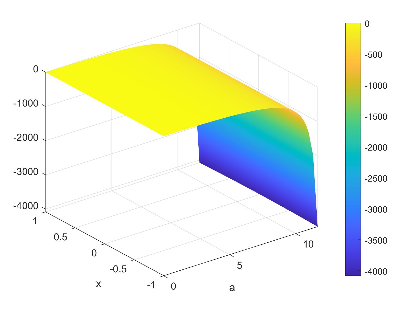
(a) $v_{0}^{\text{true}}$

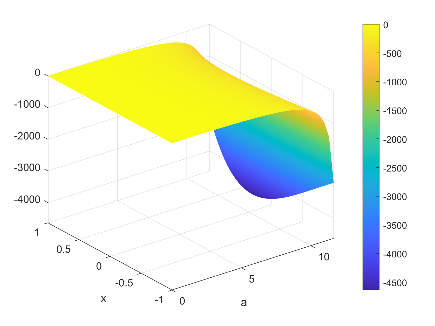
(b) $v_{0,N}^{\text{true}}$ ($N=2$)

(c) $v_{0,N}^{\text{true}}$ ($N=6$)

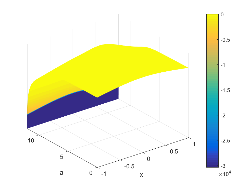
(d) $v_{0}^{\text{true}}$

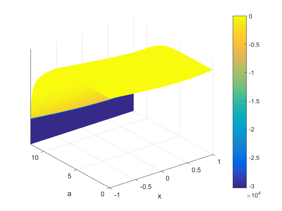
(e) $v_{0,N}^{\text{true}}$ ($N=2$)

(f) $v_{0,N}^{\text{true}}$ ($N=6$)

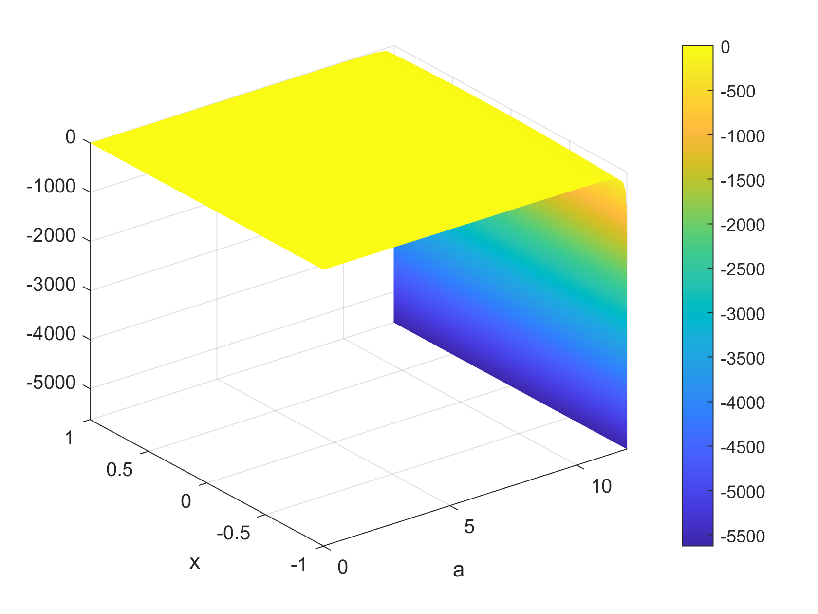
(g) $v_{0}^{\text{true}}$

(h) $v_{0,N}^{\text{true}}$ ($N=2$)

(i) $v_{0,N}^{\text{true}}$ ($N=6$)

Figure 4.1. Graphical illustrations of $v_{0}^{\text{true}}$ and $v_{0,N}^{\text{true}}$ for $N=2,6$ for Example 1 (row 1), Example 2 (row 2), and Example 3 (row 3). The mesh grid of space and age are fixed with $\Delta x=\Delta t=0.05$. By these graphical observations, $N=6$ would be the best choice for all numerical experiments because of its very high accuracy and fast-computing.

4.2. Example 1: Semiellipse initial profiles with youngster’s immobility

We begin by a numerical example with the semiellipse-shaped initial profiles near the boundary $a=0$. In particular, for $\varepsilon=0.75$, we choose

(4.1) $$u_{0}\left(a,x\right) =\frac{1}{\sqrt{2\pi}\varepsilon}\exp\left(-\frac{1}{2\varepsilon^{2}}\left(x^{2}+\left(a-0.15\right)^{2}\right)\right),$$

(4.2) $$\overline{u}_{0}\left(t,x\right) =\frac{1}{\sqrt{2\pi}\varepsilon}\exp\left(-\frac{1}{2\varepsilon^{2}}\left(x^{2}+\left(t-0.15\right)^{2}\right)\right),$$

which satisfy the compatibility condition $u_{0}\left(0,\cdot\right)=\overline{u}_{0}\left(0,\cdot\right)$; see Figure 4.2 for the graphical illustrations of the initial profile $u_{0}$. Besides, we choose $\rho=0.5$ for the net proliferation rate, and the diffusion term is chosen as

$$D\left(t,a\right)=0.03-0.03\exp\left(-\frac{\left(\frac{a_{\dagger}}{8}-a\right)^{2}}{a}\right),$$

indicating that “youngster” individuals are less mobile than newborn and old.

In our numerical experiments, we do not know the exact solutions, but we can generate data to evaluate the accuracy of the approximation. In this sense, numerical convergence can be assessed by examining numerical stability and thus, by the behavior of computed solutions at different time points and for various values of $M$. Figure 4.3 shows the computed solutions for $M=200,400,800$ and at different time points $t=2.5,5.0,7.5,10.0$. We can see that the values of the approximate solutions become more stable as $M$ increases. Moreover, the approximate solutions behave similarly at every time observation, as shown in the first row of 4.3.

To assess better the numerical stability, we plot the total population as a function of time for different values of $M=100,200,400,800$ in Figure 4.2c. The total population is formulated in Remark 3, as noted above. Figure 4.2c reveals the entire time evolution of tumor cells, with the total density significantly increasing within the first quarter of the time frame. Starting from a small amount at $t=0$ (see values of $u_{0}$ in Figure 4.2a), the total density peaks at about $t=2.1$, reaching 18 million cells/cm. Afterward, the total density gradually tends towards extinction within the next six months.

In addition, the simulation in Figure 4.7 shows that tumor cells are slightly localized along the direction of $a$ between the overpopulation and extinction phases.

Remark.

It is worth noting that since the final time observation $T$ and maximal age $a_{\dagger}$ are large, we may need huge values of $M$ to get better approximation. In fact, by the explicit numerical scheme being used, the local truncation error is of the order one.

(a) $u_{0}$ (3D)

(b) $u_{0}$ (2D)

(c) $p\left(t\right)$

Figure 4.2. Left: 3D representation of the initial data $u_{0}$ in Example 1. Middle: 2D representation of the initial data $u_{0}$ in Example 1. Right: Total population of tumor cells $p\left(t\right)$ for varying values of $M$.

(a) $M=200$

(b) $M=400$

(c) $M=800$

(d) $M=200$

(e) $M=400$

(f) $M=800$

(g) $M=200$

(h) $M=400$

(i) $M=800$

(j) $M=200$

(k) $M=400$

(l) $M=800$

Figure 4.3. Tumor cell density in Example 1 at $t=2.5,5.0,7.5,10.0$ for various values of $M$. Column 1: $M=200,\Delta t=0.05$ (36 hours). Column 2: $M=400,\Delta t=0.025$ (18 hours). Column 3: $M=800,\Delta t=0.0125$ (9 hours).

4.3. Example 2: Gaussian initial profiles with elder’s immobility

In the second example, we take into account the Gaussian initial profiles of the following form, for $\varepsilon=0.075$,

$$u_{0}\left(a,x\right)=\frac{e^{-6x^{2}}}{\varepsilon+\cosh\left(a-7\right)},\quad\overline{u}_{0}\left(t,x\right)=\frac{e^{-6x^{2}}}{\varepsilon+\cosh\left(3t-7\right)}.$$

This choice of $u_{0}$ and $\overline{u}_{0}$ satisfies the compatibility condition $u_{0}\left(0,\cdot\right)=\overline{u}_{0}\left(0,\cdot\right)$; however, compared to the choice in Example 1 (cf. (4.1) and (4.2)), the $a$ and $t$ arguments here are not interchangeable. Besides, we choose $\rho=7$ for a large net proliferation rate, and the diffusion term is chosen as

$$D\left(t,a\right)=\exp\left(-\frac{\left(t-8T\right)^{2}}{T}\right)\left(a_{\dagger}-a\right),$$

indicating that “old” individuals are very less mobile.

Our numerical results for Example 2 are presented in Figures 4.4c and 4.5. Figure 4.4c illustrates that the total population of tumor cells exhibits minimal variation when $M$ is varied between 100 to 800. Similarly, Figure 4.5 demonstrates numerical stability in the distribution of tumor cells for different values of $M$. In contrast to Example 1, these graphs are highly similar when $M$ is varied from 200 to 800, indicating that a too large $M$ is unnecessary for simulating this example.

Our simulation shows that tumor cells reach a stable state quickly, plateauing at around 2.8 thousand cells/cm across all time points (as seen in Figure 4.5). The total population, shown in Figure 4.4c, reaches its peak of 60 thousand cells/cm within three (3) months from an initial total population of about 3 thousand cells. Subsequently, the total population appears to stabilize but gradually declines over time.

(a) $u_{0}$ (3D)

(b) $u_{0}$ (2D)

(c) $p\left(t\right)$

Figure 4.4. Left: 3D representation of the initial data $u_{0}$ in Example 2. Middle: 2D representation of the initial data $u_{0}$ in Example 2. Right: Total population of tumor cells $p\left(t\right)$ for varying values of $M$.

(a) $M=200$

(b) $M=400$

(c) $M=800$

(d) $M=200$

(e) $M=400$

(f) $M=800$

(g) $M=200$

(h) $M=400$

(i) $M=800$

(j) $M=200$

(k) $M=400$

(l) $M=800$

Figure 4.5. Tumor cell density in Example 2 at $t=2.5,5.0,7.5,10.0$ for various values of $M$. Column 1: $M=200,\Delta t=0.05$ (36 hours). Column 2: $M=400,\Delta t=0.025$ (18 hours). Column 3: $M=800,\Delta t=0.0125$ (9 hours).

4.4. Example 3: Hump-shaped initial profiles

In this last example, we examine the explicit Fourier-Klibanov scheme for our Gompertz system with the following initial conditions:

$$u_{0}\left(a,x\right)=\frac{1}{\sqrt{2\pi}\varepsilon}\left[2-\sin\left(\frac{\pi}{4}\left(a-3\right)\right)\right]\exp\left(-\left(x-0.25\right)^{2}\right),$$

$$\overline{u}_{0}\left(t,x\right)=\frac{1}{\sqrt{2\pi}\varepsilon}\left[2-\sin\left(\frac{\pi}{4}\left(t-3\right)\right)\right]\exp\left(-\left(x-0.25\right)^{2}\right),$$

where $\varepsilon=0.5$. Cf. Figure 4.6b, these functions model well the hump-shaped profiles in the plane of $x$ and $a$. It is also understood that there are two adjacent tumor distributions presented in the sampled brain tissue. Using the proposed scheme, we look for the dynamics of these tumor cell distributions with $\rho=0.36$ being the net proliferation rate and

$$D\left(t,a\right)=\exp\left(-\left(t-2T\right)^{2}-\left(a-2a_{\dagger}\right)^{2}\right).$$

By the choice of $D\left(t,a\right)$ above, only the “elders” diffuse, but very slowly, at the final time observation.

We present our numerical findings for this example through: Figure 4.7 illustrates the tumor cell density, while Figure 4.6c depicts the total population. Based on our numerical observations, we find that the approximation is very stable as $M$ increases. The curves representing the total population in Figure 4.6c almost coincide, indicating a very good accuracy in the macroscopic sense. However, it is important to note that the accuracy of the approximation decreases as we move further away from the initial point, particularly towards the final time observation; see again Figure 4.6c.

The simulation provides some insights into the behavior of tumor cells, as depicted in Figures 4.6c and 4.7. Starting with 3 thousand cells/cm, the total population gradually increases and reaches its peak of approximately 44 thousand cells/cm in a span of 10 months. The population somehow reaches a steady state between the third and sixth months. Similar to Example 2, the distribution of tumor cells has a modest peak, indicating that a too large $M$ is not required for numerical stability at all time points.

Furthermore, Figure 4.7 shows the development and spread of tumor cells from the original two distributions as both age and time evolve. At certain time points, new tumor cells emerge and gradually propagate to merge with the existing “older” distribution.

(a) $u_{0}$ (3D)

(b) $u_{0}$ (2D)

(c) $p\left(t\right)$

Figure 4.6. Left: 3D representation of the initial data $u_{0}$ in Example 3. Middle: 2D representation of the initial data $u_{0}$ in Example 3. Right: Total population of tumor cells $p\left(t\right)$ for varying values of $M$.

(a) $M=200$

(b) $M=400$

(c) $M=800$

(d) $M=200$

(e) $M=400$

(f) $M=800$

(g) $M=200$

(h) $M=400$

(i) $M=800$

(j) $M=200$

(k) $M=400$

(l) $M=800$

Figure 4.7. Tumor cell density in Example 3 at $t=2.5,5.0,7.5,10.0$ for various values of $M$. Column 1: $M=200,\Delta t=0.05$ (36 hours). Column 2: $M=400,\Delta t=0.025$ (18 hours). Column 3: $M=800,\Delta t=0.0125$ (9 hours).

5. Conclusions

In this work, we have presented a new numerical approach to solve the age-structured population diffusion problem of Gompertz type. Our approach relies on a combination of the recently developed Fourier-Klibanov method and the explicit finite difference method of characteristics. The notion is that exploiting suitable transformations, the Gompertz model of interest turns to a third-order nonlinear PDE. Then, the Fourier-Klibanov method is applied to derive a coupled transport-like PDE system. This system is explicitly approximated by the finite difference operators of time and age.

In this work, we have focused on the numerics rather than the theory. It remains to show the rate of convergence of the explicit scheme under particular smoothness conditions of the involved parameters and the true solution. Besides, it is still open in this age-dependent Gompertz mode that if we have the non-negativity of the initial data, the whole solution will follow.

As readily expected, the explicit finite difference method is conditionally stable. Thus, the implicit scheme should be investigated in the upcoming research. We also want to extend the applicability of the method to nonlinear heterogeneous problems in multiple dimensions.

References

• [1] G. Akrivis, M. Crouzeix, and V. Thomée. Numerical methods for ultraparabolic equations. Calcolo, 31(3-4):179–190, 1994.
• [2] A. Ashyralyev and S. Yilmaz. Modified Crank-Nicholson difference schemes for ultra-parabolic equations. Computers & Mathematics with Applications, 64(8):2756–2764, 2012.
• [3] B. P. Ayati, G. F. Webb, and A. R. A. Anderson. Computational methods and results for structured multiscale models of tumor invasion. Multiscale Modeling & Simulation, 5(1):1–20, 2006.
• [4] W.-S. Cheung and J. Ren. Discrete non-linear inequalities and applications to boundary value problems. Journal of Mathematical Analysis and Applications, 319(2):708–724, 2006.
• [5] M. Iannelli and G. Marinoschi. Approximation of a population dynamics model by parabolic regularization. Mathematical Methods in the Applied Sciences, 36(10):1229–1239, 2012.
• [6] R. Jaroudi, F. Åström, B. T. Johansson, and G. Baravdish. Numerical simulations in 3-dimensions of reaction-diffusion models for brain tumour growth. International Journal of Computer Mathematics, 97(6):1151–1169, 2019.
• [7] V. A. Khoa, T. N. Huy, L. T. Lan, and N. T. Y. Ngoc. A finite difference scheme for nonlinear ultra-parabolic equations. Applied Mathematics Letters, 46:70–76, 2015.
• [8] V. A. Khoa, M. V. Klibanov, and L. H. Nguyen. Convexification for a three-dimensional inverse scattering problem with the moving point source. SIAM Journal on Imaging Sciences, 13(2):871–904, 2020.
• [9] M.-Y. Kim and E.-J. Park. Mixed approximation of a population diffusion equation. Computers & Mathematics with Applications, 30(12):23–33, 1995.
• [10] M. V. Klibanov. Convexification of restricted Dirichlet-to-Neumann map. Journal of Inverse and Ill-posed Problems, 25(5), 2017.
• [11] M. V. Klibanov, A. E. Kolesov, A. Sullivan, and L. Nguyen. A new version of the convexification method for a 1D coefficient inverse problem with experimental data. Inverse Problems, 34(11):115014, 2018.
• [12] M. V. Klibanov, T. T. Le, and L. H. Nguyen. Numerical solution of a linearized travel time tomography problem with incomplete data. SIAM Journal on Scientific Computing, 42(5):B1173–B1192, 2020.
• [13] M. V. Klibanov, J. Li, and W. Zhang. Numerical solution of the 3-D travel time tomography problem. Journal of Computational Physics, 476:111910, 2023.
• [14] I. V. Kuznetsov and S. A. Sazhenkov. Genuinely nonlinear impulsive ultra-parabolic equations and convective heat transfer on a shock wave front. IOP Conference Series: Earth and Environmental Science, 193:012037, 2018.
• [15] T. T. Le and L. H. Nguyen. The gradient descent method for the convexification to solve boundary value problems of quasi-linear PDEs and a coefficient inverse problem. Journal of Scientific Computing, 91(3), 2022.
• [16] L. Lorenzi. An abstract ultraparabolic integrodifferential equation. Le Matematiche, 53(2):401–435, 1998.
• [17] M. D. Marcozzi. Extrapolation discontinuous Galerkin method for ultraparabolic equations. Journal of Computational and Applied Mathematics, 224(2):679–687, 2009.
• [18] J. D. Murray. Continuous Population Models for Single Species. In Interdisciplinary Applied Mathematics, volume 17, pages 1–43. Springer, New York, 1993.
• [19] E. Ozugurlu. A note on the numerical approach for the reaction-diffusion problem to model the density of the tumor growth dynamics. Computers & Mathematics with Applications, 69(12):1504–1517, 2015.
• [20] Y. Qin. Integral and Discrete Inequalities and Their Applications. Springer International Publishing, 2016.
• [21] J. W. Sinko and W. Streifer. A new model for age-size structure of a population. Ecology, 48(6):910–918, 1967.
• [22] D. Wodarz and N. L. Komarova. Dynamics of Cancer. World Scientific, 2014.