How to account for behavioural states in step-selection analysis: a model comparison

Abstract

1. Step-selection models are widely used to study animals’ fine-scale habitat selection based on movement data. Resource preferences and movement patterns, however, can depend on the animal’s unobserved behavioural states, such as resting or foraging. This is ignored in standard (integrated) step-selection analyses (SSA, iSSA). While different approaches have emerged to account for such states in the analysis, the performance of such approaches and the consequences of ignoring the states in the analysis have rarely been quantified.

2. We evaluated the recent idea of combining hidden Markov chains and iSSA in a single modelling framework. The resulting Markov-switching integrated step-selection analysis (MS-iSSA) allows for a joint estimation of both the underlying behavioural states and the associated state-dependent habitat selection. In an extensive simulation study, we compared the MS-iSSA to both the standard iSSA and a classification-based iSSA (i.e., a two-step approach based on a separate prior state classification). We further compared the three approaches in a case study on fine-scale interactions of simultaneously tracked bank voles (Myodes glareolus).

3. The simulation study illustrates that standard iSSAs lead to erroneous conclusions due to both biased estimates and unreliable p-values when ignoring underlying behavioural states. We found the same for iSSAs based on prior state-classifications, as they ignore misclassifications and classification uncertainties. The MS-iSSA, on the other hand, performed well in parameter estimation and decoding of behavioural states. In the bank-vole case study, the MS-iSSA was able to distinguish between an inactive and active state, but results highly varied between individuals.

4. MS-iSSA provides a flexible framework to study state-dependent habitat selection. It defines states on both selection and movement patterns and accounts for uncertainties in the corresponding state process. To facilitate its use, we implemented the MS-iSSA approach in the R package msissa.

Keywords: animal movement, fine-scale interactions, habitat selection, hidden Markov models, Markov-switching regression, movement behaviour, state-switching, integrated step-selection analysis

1 Introduction

Combining animal movement and environmental data, step-selection analysis (SSA) and its extension, the integrated step-selection analysis (iSSA), build a popular framework for studying animals’ fine-scale habitat selection, while also taking the movement capacity of the animal into account (Fortin et al.,, 2005; Forester et al.,, 2009; Avgar et al.,, 2016; Northrup et al.,, 2022). Essentially, SSA and iSSA are used to explain the animals’ space use based on possible preferences for or avoidance of environmental features, accounting for spatial limitations that the animals’ movement process imposes on availability. ISSA has successfully been applied, for example, to analyse elk response to roads (Prokopenko et al.,, 2017), to study the effects of artificial nightlight on predator–prey dynamics of cougars and deer (Ditmer et al.,, 2021), and to model space use of Cape vultures in the context of wind energy development (Cervantes et al.,, 2023). Besides conventional habitat use, SSA has also proven suitable for detecting interactions such as avoidance or attraction between simultaneously tracked individuals (Schlägel et al.,, 2019).

For parameter estimation, SSA and iSSA use a conditional logistic regression for case-control designs to compare the characteristics of observed, i.e. used steps against the covariates of alternative steps available at a given time point. In this context, a step is the straight-line segment connecting two consecutive locations sampled at regular time intervals and is usually described by the step length and turning angle, i.e. the directional change (Fortin et al.,, 2005). The covariates usually correspond to features of the steps’ end point, e.g. vegetation or snow cover (Stratmann et al.,, 2021), but can also refer to characteristics along the step, e.g. the presence of roads on the path (Prokopenko et al.,, 2017). What is considered to be available at a given time point depends on the assumptions made about the animals’ movement capacities and/or typical, i.e. habitat-selection-free movement patterns. This usually translates to assumptions about the animals’ step length and turning angle distribution (e.g. gamma and von Mises distributions). Tentative parameter estimates for these distributions can be estimated from observed steps. These estimates are biased because movement is restricted by habitat selection. A correction for the tentative parameters can be estimated using iSSA (Avgar et al.,, 2016; Fieberg et al.,, 2021).

While (i)SSAs seem suitable in numerous instances, it has recently been argued that fine-scale habitat selection, resource requirements, and selection-free movement patterns might depend on the animal’s behavioural modes such as resting or foraging (illustrated in Figure 1). Ignoring such states in the analysis might thus lead to biased results and misleading conclusions (Roever et al.,, 2014; Suraci et al.,, 2019). With telemetry-based location data, however, the underlying behavioural states are usually unobserved. Therefore, it has been suggested to first classify the movement data into different states, e.g. based on hidden Markov models (HMMs, Zucchini et al.,, 2016), and to split the step observations accordingly into state-specific data sets, which can then be used to fit state-specific (i)SSAs in a second step (Roever et al.,, 2014; Karelus et al.,, 2019; Picardi et al.,, 2022). This two-step approach, hereafter named TS-(i)SSA, accounts for the unobserved state structure and is convenient as it can be based on existing software implementations. It has, however, two major drawbacks. First, the state classification is purely based on movement patterns without considering habitat selection. Thus, habitat selection and selection-independent movement processes can be confounded when defining the states. This can affect the validity of the state classification and can lead to a bias in the estimated movement and selection parameters (Prima et al.,, 2022). Second, the uncertainty in the HMM state classification is completely ignored in the follow-up (i)SSA. This can again lead to biased movement and (habitat) selection coefficients, as misclassification can occur. Furthermore, confidence intervals and standard p-values are no longer reliable as the uncertainty of both the HMM parameter estimation and the state classification are not taken into account. Consequently, also the TS-iSSA might lead to biased results and misleading conclusions. How serious this is in practice, however, has rarely been quantified. Prima et al., (2022) evaluated a population-level version of the TS-iSSA in a simulation study and found good classification and prediction performances in the scenarios considered, but also biased parameter estimates. However, as they focused on the population level, they did not provide results on the variation, uncertainty quantification and estimation accuracy of the individually fitted TS-iSSA models.

Figure 1: Illustration of how behavioural states can affect animals habitat selection and movement patterns. The state “foraging” is related to search for food such as small insects in an open landscape, while the state “resting” is associated to a retreat in its shelter. Usually, the behavioural states are unobserved, thus hidden, and serially correlated. This structure corresponds to the basic dependence structure of a Markov-switching step-selection model.

The above mentioned problems could be avoided by combining step selection models and hidden Markov chains (as used in HMMs) in a single model to allow for a joint estimation of the underlying state, habitat selection and selection-free movement processes. Similar as Nicosia et al., (2017) and Prima et al., (2022), we therefore consider a Markov-switching integrated step-selection analysis (MS-iSSA, also called HMM-SSA) which renders a prior state classification unnecessary. All model parameters are jointly estimated using a case-control Markov-switching conditional logistic regression framework. In our implementation, we use a numerical maximum likelihood estimation and constrain all parameters to their natural parameter space to avoid problems in model interpretation (e.g. a negative shape parameter for an assumed gamma distribution for step length). For state decoding, we consider the well-known Viterbi algorithm, which computes the most likely state sequence underlying the data given the fitted model.

The aim of this paper is two-fold. First, we provide a broad overview of the MS-iSSA framework by discussing the underlying movement model, its relation to alternative approaches (iSSA, TS-iSSA, HMMs) and, most importantly, its practical implementation, which we further facilitate through release as an R package. Second, we investigate whether and to what extent either the complete neglect of underlying states in the analysis (iSSA) or their incorporation by a prior HMM-based state classification (TS-iSSA) affects the estimation results compared to the MS-iSSA approach. For this, we use an extensive simulation study to compare the estimation and, if applicable, classification performance of iSSAs, TS-iSSAs and MS-iSSAs in three state-switching scenarios. Thereby, we showcase different ways in which behavioural states could influence the animals’ movement decisions. A supplementary simulation covers a scenario without underlying state-switching. We further compare the three approaches in a case study on fine-scale interactions of bank voles (Myodes glareolus), which are small ground-dwelling rodents. Using a movement data set of synchronously tracked individuals, as analysed in Schlägel et al., (2019), we test whether MS-iSSAs can detect meaningful biological states and whether they provide new insights into interactions, such as attraction, avoidance, or neutrality towards other conspecifics compared to iSSAs.

2 Methods

2.1 Markov-switching step-selection model

We use $\{\mathbf{x}_{0,1},\mathbf{x}_{0,2},\ldots,\mathbf{x}_{0,T}\}$ to denote the sequence of two-dimensional animal locations observed at regular time intervals, which forms the observed movement track. Conditional on the previous location $\mathbf{x}_{0,t-1}$, a step from the current location $\mathbf{x}_{0,t}$ to the next location $\mathbf{x}_{0,t+1}$, is characterised by its step length $l_{0,t+1}$, i.e. the straight-line distance between the two consecutive locations, and its turning angle $\alpha_{0,t+1}$, i.e. the directional change. The corresponding covariate vector $\mathbf{Z}_{0,t+1}$ stores the feature values of the step, and we use $\mathbf{Z}$ to denote the collection of covariate values for all possible location in the given area.

In the Markov-switching step-selection model, we assume the observed steps to be driven by an underlying hidden state sequence $\{S_{1},S_{2},\ldots,S_{T}\}$ with $N$ discrete states. Thus, each state variable $S_{t}$ at time $t$ can take one of $N$ state values ($S_{t}\in\{1,\ldots,N\}$). These states serve as proxies for the unobserved behavioural modes of the animal that influence its movement and habitat selection (illustrated in Figure 1). We assume the state sequence to be a homogeneous $N$-state Markov chain, characterised by its transition probabilities $\gamma_{ij}=\Pr(S_{t}=j\mid S_{t-1}=i)$ to switch from state $i$ to state $j$, summarised in the $N\times N$ transition probability matrix $\bm{\Gamma}$, and the initial state distribution $\bm{\delta}$ which contains the probabilities to start in a certain state.

Each state $i$ ($i=1,\ldots,N$) is associated to a state-dependent density $f_{i}$ generating the next location. Its functional form is similar to the basic step-selection model (Forester et al.,, 2009), but with movement and habitat selection parameters being state-dependent. Thus, conditional on locations $\mathbf{x}_{0,t-1}$ and $\mathbf{x}_{0,t}$, and covariates $\mathbf{Z}$, the current state $S_{t}=i$ determines the following distribution for a step to location $\mathbf{x}_{0,t+1}$:

$$f_{i}(\mathbf{x}_{0,t+1}\mid\mathbf{x}_{0,t},\mathbf{x}_{0,t-1},\mathbf{Z};\bm{\theta}_{i},\bm{\beta}_{i}) =\cfrac{\overbrace{\vphantom{\mathbf{Z(\mathbf{x})}^{\top}}\phi(\mathbf{x}_{0,t+1}\mid\mathbf{x}_{0,t},\mathbf{x}_{0,t-1};\bm{\theta}_{i})}^{\begin{subarray}{c}\text{selection-free}\\ \text{movement kernel}\end{subarray}}\cdot\overbrace{\omega(\mathbf{Z}_{0,t+1};\bm{\beta}_{i})}^{\begin{subarray}{c}\text{movement-free}\\ \text{selection function}\end{subarray}}}{\underbrace{\int_{\mathbf{\tilde{x}}\in\mathcal{D}}\phi(\mathbf{\tilde{x}}\mid\mathbf{x}_{0,t},\mathbf{x}_{0,t-1};\bm{\theta}_{i})\cdot\omega(\mathbf{\tilde{Z}};\bm{\beta}_{i})d\mathbf{\tilde{x}}}_{\text{normalising constant}}}$$

The density consists of three components: i) The movement kernel $\Phi(\cdot)$ describes the space use in a homogeneous landscape and is usually defined in terms of step length $l_{0,t+1}$ (e.g. gamma distribution) and turning angle $\alpha_{0,t+1}$ (e.g. von Mises distribution). The corresponding state-dependent parameters for state $i$ are summarised in the movement parameter vector $\bm{\theta}_{i}$; ii) The movement kernel is weighted by the movement-free selection function $\omega(\cdot)$ which indicates a possible selection for or against the covariates in $\mathbf{Z}_{0,t+1}$. It is usually assumed to be a log-linear function of the (state-dependent) selection coefficient vector $\bm{\beta}_{i}$,

$$\omega(\mathbf{Z}_{0,t+1};\bm{\beta}_{i})=\exp\left(\mathbf{Z}_{0,t+1}^{\top}\bm{\beta}_{i}\right),$$

where a positive selection coefficient value indicates preference for, and a negative value avoidance of a corresponding covariate; iii) The integral in the denominator ensures that $f_{i}$ integrates to one. Usually, it is analytically intractable and must therefore be approximated, for example, using numerical integration methods. We provide an example of state-dependent step-selection densities in a $2$-state scenario in Figure S1 (Supplementary Material).

There are important relations between the Markov-switching step-selection model and two alternative movement models: i) If all states share the same parameters, i.e. $\bm{\theta}_{1}=\ldots=\bm{\theta}_{N}$ and $\bm{\beta}_{1}=\ldots=\bm{\beta}_{N}$, or if the number of states is set to one, i.e. $N=1$, the model reduces to the basic step-selection model without state-switching (Forester et al.,, 2009); ii) If all selection coefficients are equal to zero, i.e. $\bm{\beta}_{1}=\ldots=\bm{\beta}_{N}=\mathbf{0}$, the model reduces to a basic movement HMM (Langrock et al.,, 2012, Patterson et al.,, 2017) with state-dependent step length and turning angle distributions as implied by the movement kernel $\phi(\cdot)$ but without habitat selection. These relations are very convenient, for example in the context of model comparison and model selection, as it allows the use of standard tests or information criteria to select between these three candidate models.

We can simplify the step-selection density $f_{i}$ by assuming step length to follow a distribution from the exponential family (with support on non-negative real numbers, e.g. a gamma distribution) and turning angle to follow either a uniform or von Mises distribution with fixed mean (Avgar et al.,, 2016; Nicosia et al.,, 2017). In this case, the product of the movement kernel $\phi(\cdot)$ and the exponential selection function $\omega(\cdot)$ is proportional to a single log-linear function of the corresponding model parameters and $f_{i}$ reduces to:

$$f_{i}(\mathbf{x}_{0,t+1}\mid\mathbf{x}_{0,t},\mathbf{x}_{0,t-1},\mathbf{Z};\bm{\theta}_{i},\bm{\beta}_{i}) =\genfrac{}{}{}{}{\raisebox{3.0pt}{$\exp\left(\mathbf{C}_{0,t+1}^{\top}\bm{\theta}_{i}+\mathbf{Z}_{0,t+1}^{\top}\bm{\beta}_{i}-\log(l_{0,t+1})\right)$}}{\raisebox{-3.0pt}{$\displaystyle\int_{\mathbf{\tilde{x}}\in\mathcal{D}}\exp\left(\mathbf{\tilde{C}}^{\top}\bm{\theta}_{i}+\mathbf{\tilde{Z}}^{\top}\bm{\beta}_{i}-\log(\tilde{l})\right)d\mathbf{\tilde{x}}$}}.$$

The vector $\mathbf{C}_{0,t+1}$ can be interpreted as a movement covariate vector that contains different step length and turning angle terms. Its exact form depends on the chosen step length and turning angle distributions (Table S1, see also Nicosia et al.,, 2017). For example, for gamma-distributed step length and von-Mises-distributed turning angles with mean zero, we have $\mathbf{C}_{0,t+1}=(\log(l_{0,t+1}),-l_{0,t+1},\allowbreak\cos(\alpha_{0,t+1}))^{\top}$. The corresponding state-dependent movement coefficient vector is $\bm{\theta}_{i}=(k_{i}-1,r_{i},\kappa_{i})^{\top}$ with $k_{i}$ and $r_{i}$ being the shape and rate parameter of the gamma-distribution belonging to state $i$, respectively, and $\kappa_{i}$ being the state-dependent concentration parameter of the von-Mises distribution. Thus, in this reduced representation of the step-selection density $f_{i}$, the parameterisation of the movement kernel might differ from the commonly used parameterisation of the corresponding step and angle distributions (e.g. $k_{i}-1$ instead of $k_{i}$), but there is a direct relationship between the two (Table S1 and S2). The negative log step length included in the exponential function is necessary to correctly represent the movement kernel in a Cartesian coordinate system.

The reduced form of $f_{i}$ is very convenient. Justified by the law of large numbers, it allows for a joint parameter estimation of the state, movement and selection parameters based on a Markov-switching conditional logistic regression for case-control designs with $M$ control, i.e. available, locations per observed, i.e. used, location (Nicosia et al.,, 2017, see also Avgar et al., 2016 for step-selection models without state-switching). This forms the basis for the MS-iSSA.

2.2 Markov-switching integrated step-selection analysis

The MS-iSSA workflow is similar to the one of the iSSA. For each observed step, we choose $M$ control steps, e.g. using a suitable proposal distribution for step length and turning angle, respectively, and extract the corresponding habitat and movement covariate values. This builds the case-control data set. The model parameters are then estimated using a Markov-switching conditional logistic regression, i.e. a conditional logistic regression in which the regression coefficients depend on an underlying latent Markov chain. In our implementation, we use the forward algorithm, which is well-known especially in the context of HMMs (Zucchini et al.,, 2016) to efficiently evaluate the corresponding likelihood. This allows for a numerical maximum likelihood estimation based on standard optimisation procedures such as nlm in R (R Core Team,, 2022). Afterwards, it is possible to decode the states, for example, using the Viterbi algorithm (Viterbi,, 1967), which calculates the most likely sequence of states given the fitted model and the case-control data.

More precisely, for each step from location $\mathbf{x}_{0,t}$ to $\mathbf{x}_{0,t+1}$ ($t=2,\ldots,T-1$), we have a choice set $\tilde{\mathbf{x}}_{t+1}=\{\mathbf{x}_{0,t+1},\mathbf{x}_{1,t+1},\ldots,\mathbf{x}_{M,t+1}\}$ that includes the observed and the $M$ control locations for the end point of the step. Usually, the control locations are randomly drawn from a suitable proposal distribution for step length and turning angle (Forester et al.,, 2009). However, it is also possible to use a grid or a mesh (Guillen et al.,, 2023). Here the devil is in the detail, as depending on the sampling procedure, the interpretation of the models’ movement coefficients might differ (see Section S2 in the Supplementary Material). The interpretation of the selection coefficients, however, remain unaffected.

In the Markov-switching conditional logistic regression, we model the state-dependent choice probability $p_{0ti}$ of choosing the observed location $\mathbf{x}_{0,t+1}$ from the choice set $\tilde{\mathbf{x}}_{t+1}$ given the current state $S_{t}=i$, as:

$$p_{0ti}(\mathbf{x}_{0,t+1}|\tilde{\mathbf{x}}_{t+1},\mathbf{C},\mathbf{Z};\bm{\theta}_{i},\bm{\beta}_{i})=\genfrac{}{}{}{}{\raisebox{2.0pt}{$\exp\left(\mathbf{C}_{0,t+1}^{\top}\bm{\theta}_{i}+\mathbf{Z}_{0,t+1}^{\top}\bm{\beta}_{i}\right)$}}{\raisebox{-2.0pt}{$\sum_{m=0}^{M}\exp\left(\mathbf{C}_{m,t+1}^{\top}\bm{\theta}_{i}+\mathbf{Z}_{m,t+1}^{\top}\bm{\beta}_{i}\right)$}},$$

with $\mathbf{C}_{m,t+1}$ and $\mathbf{Z}_{m,t+1}$ being the movement and habitat covariate vectors belonging to location $\mathbf{x}_{m,t+1}$ for $m=0,\ldots,M$. This case-control step-selection probability is closely related to direct numerical integration, which offers an alternative way to approximate the step-selection density $f_{i}$. We derive the likelihood of the Markov-switching conditional logistic regression by plugging $p_{0ti}$ ($i=1,\ldots,N$) into the HMM likelihood (Zucchini et al.,, 2016),

$$\mathcal{L}(\bm{\theta},\bm{\beta};\tilde{\mathbf{x}}_{3},\tilde{\mathbf{x}}_{4},\ldots,\tilde{\mathbf{x}}_{T},\mathbf{C},\mathbf{Z}) =\bm{\delta}^{\top}\mathbf{P}(\tilde{\mathbf{x}}_{3})\bm{\Gamma}\mathbf{P}(\tilde{\mathbf{x}}_{4})\bm{\Gamma}\cdots\bm{\Gamma}\mathbf{P}(\tilde{\mathbf{x}}_{T})\bm{1},$$

where $\mathbf{P}(\tilde{\mathbf{x}}_{t})=\text{diag}(p_{0t1},\ldots,p_{0tN})$ is a diagonal matrix including the state-dependent step-selection probabilities, $\bm{\Gamma}$ and $\bm{\delta}$ are the transition probability matrix and the initial distribution of the underlying Markov chain, respectively, and $\mathbf{1}$ is an $N$-dimensional vector of ones. We can then estimate the model parameters using a numerical maximisation of the log-likelihood (for details, see Zucchini et al.,, 2016). In our implementation, we restrict the movement parameters to always remain in their natural parameter space, e.g. the shape and rate parameters of the gamma distribution are always greater than zero.

For initialisation, the numerical maximisation requires a set of starting values for the model parameters. To avoid ending up in a local maximum of the log-likelihood, it is necessary to test several sets of starting values, for example by randomly drawing values for each model parameter. We discuss this in more detail in Section S3 in the Supplementary Material.

2.3 Two-step approach

The TS-iSSA is based on the same idea as the MS-iSSA. However, the TS-iSSA relies on a prior classification of the movement data into different movement states. Thus, in a first step, an $N$-state HMM with state-dependent step length and turning angle distributions as defined for the movement kernel is fitted to the data, e.g. using a gamma distribution for step length and a von Mises distribution for turning angles. Then, the Viterbi algorithm is used to assign each observed step to one of the $N$ HMM movement states. Alternatively, local state decoding can be used. In the second step, state-specific (i)SSAs are fitted to the state-specific data using a case-control design and conditional logistic regression (e.g. Roever et al.,, 2014; Karelus et al.,, 2019). The control steps for the state-specific case-control data sets are thereby sampled based on the respective state-dependent HMM step length and turning angle distributions.

2.4 Simulation Study

We used a simulation study with three state-switching scenarios to evaluate the performance of our MS-iSSA approach and to demonstrate possible consequences of either ignoring the underlying latent states in the traditional iSSA or ignoring the uncertainty of prior state-decoding in the TS-iSSA. For each scenario, we generated movement data from a Markov-switching step-selection model with $2$ states and state transition probabilities $\gamma_{11}=\gamma_{22}=0.9$. A realisation of a Gaussian random field with covariance $\sigma^{2}=1$ and range $\phi=10$, computed using the function grf from the R-package geoR (Ribeiro Jr et al.,, 2022), served as the habitat covariate $\mathbf{Z}$ (Figure S2). For the movement kernel, we used state-dependent gamma and zero-mean von Mises distributions to model step length and turning angle, respectively (Figure 2).

Table 1 summarises the movement and selection parameters for each of the three simulation scenarios. Scenario 1 is chosen to represent a typical inactive-active scenario in which the first state (“inactive” state) is associated to small step length, less directive movement and no selection, while the second state (“active” state) corresponds to larger step length, more directed movement and attraction to the landscape feature $\mathbf{Z}$. The second and the third scenarios cover the rather extreme cases in which either the selection or the movement parameters are shared across states: In Scenario 2 (“switching preferences”), the two states only differ in their selection patterns with avoidance of the feature in state 1, and attraction to the feature in state 2. In Scenario 3 (“HMM”), only the movement patterns differ across states while there is no selection for or against the landscape feature in either state. This corresponds to a basic movement HMM (see Section 2.1). To check the robustness of the MS-iSSA, in Section S5.2 of the Supplementary Material we additionally cover a fourth scenario without state-switching in which the data are generated based on a standard step-selection model. Furthermore, to check the influence of the spatial variation in the habitat feature on the estimation results, we also considered a second landscape feature map which was a realisation of a Gaussian random field with covariance $\sigma^{2}=1$ and range $\phi=50$ (Section S5.3 in the Supplementary Material).

	state 1				state 2
	select. fun.	movement kernel			select. fun.	movement kernel
scenario	$\beta_{1}$	$k_{1}$	$r_{1}$	$\kappa_{1}$	$\beta_{2}$	$k_{2}$	$r_{2}$	$\kappa_{2}$
1 (active-inactive)	$0.00$	1.20	1.25	0.30	$2.00$	2.50	0.29	1.00
2 (switching preferences)	$-2.00$	2.50	0.29	1.00	$2.00$	2.50	0.29	1.00
3 (HMM)	$0.00$	1.20	1.25	0.30	$0.00$	2.50	0.29	1.00
4 (iSSA, Supp. Mat.)	$2.00$	2.50	0.29	1.00	$-$	–	–	–

Table 1: Overview of the underlying Markov-switching step-selection model parameters for each simulation scenario. The selection coefficients $\beta_{i}$ for state $i$ ($i=1,2$), describe the habitat selection and belong to the selection function of the model. The movement kernel parameter vector $\bm{\theta}_{i}$ includes the shape $k_{i}$ and rate $r_{i}$ of gamma distribution for step length and the concentration parameter $\kappa_{i}$ of the von-Mises distribution for turning angles. Scenario 4 does not include any state-switching and is covered in the Supplementary Material.

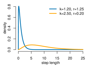
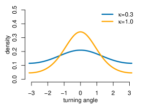
Figure 2: Gamma and von Mises distributions for step length and turning angle, respectively, which are used in the simulation study to form the state-dependent movement kernels of the two states. The corresponding parameters are denoted by $k$ (shape), $r$ (rate) and $\kappa$ (concentration). The distributions of state $2$ are shown in orange. The distributions for state $1$ depend on the simulation scenario: In Scenario 2, both states share the same movement kernel and thus, the distributions in orange are also used for state $1$; in the other two Scenarios 1 and 3, the distributions in blue are used for state $1$.

In each of the $100$ simulation runs per scenario, we simulated movement paths of length $T=1000$ from the corresponding Markov-switching step-selection model and then applied 2-state MS-iSSAs, 2-state TS-iSSAs and iSSAs to corresponding case-control data sets with $M=20$, $M=100$ and $M=500$ randomly drawn control steps per observed step, respectively. We use different numbers of control locations $M$ to check whether the parameter estimates converge to stable values. For the control steps, we used a uniform distribution for turning angles and a proposal gamma distribution for step length, respectively (Section S2). For model selection purposes, we further estimated the parameters of a $2$-state MS-iSSA with movement but without habitat covariates. This corresponds to a basic movement HMM, but fitted to the same case-control data as the candidate models. All models were implemented in R (R Core Team,, 2022). For the iSSA, we used the clogit-function of the survival package (Therneau,, 2020). After parameter estimation, we computed AIC and BIC for model selection (Burnham and Anderson,, 2002) and the basic p-values of the estimated selection coefficients. For the TS-iSSA and MS-iSSA we further computed the state missclassification rate, i.e. the percentage of states that were not correctly classified using the Viterbi algorithm. These metrics were used to evaluate the estimation and classification accuracy of the candidate models, and to assess the performance of standard model selection procedures.

2.5 Case Study on bank vole interactions

To illustrate the use of MS-iSSAs on empirical data, we applied them to movement data of synchronously tracked bank vole individuals (Myodes glareolus) as analysed in Schlägel et al., (2019). The data set contains $6$-minute locations of $n=28$ individuals split into $8$ groups, i.e. replicates, with $2$ males and $1$-$2$ females each. The individuals within a replicate were synchronously tracked in fenced quadratic outdoor enclosures of $2500\text{m}^{2}$ for $3-5$ days using collars with small radio telemetry transmitters (1.1 g, BD‐2C, Holohil Systems Ltd., Canada) and a system of automatic receiving units (Sparrow systems, USA). For bank vole individuals tracked under natural conditions, the estimated home range sizes were on average $2029.18\text{m}^{2}$ with a core area of $549.23\text{m}^{2}$ (Schirmer et al.,, 2019). Thus, the size of the enclosures allowed the individuals to express their natural movement and space use. Due to daily system maintenance, locations were missing for approximately one hour per day. Otherwise, movement paths were complete. This resulted in $602$–$1,200$ locations per individual split into $3-5$ bursts of around $23$ hours each.

To study interactions between the bank vole individuals, i.e. attraction, avoidance or neutral behaviour towards each other, Schlägel et al., (2019) applied SSAs to each individual of each replicate, respectively, using occurrence estimates of the conspecifics as covariates. The occurrence estimate of an individual provides a map of the individual’s space use during a certain time window, indicating areas of higher and lower probability of occurrence during that time period. It is estimated from the discrete sample of observed locations through kriging (Fleming et al.,, 2016). To account for the movement of individuals, occurrence estimates are computed using a rolling time window (here $4$ hours).

The analysis focused on interactions between males and females: Males were expected to mainly show attraction towards females, while females could show any of the three behaviours depending on their reproductive state (Schlägel et al.,, 2019). The authors suggested that the relatively large number of non‐significant interaction coefficients, especially found for male interactions with females, might be caused by unobserved mixtures of different underlying behavioural modes. Bank voles are polyphasic with resting phases of approximately $3\text{h}$ and active phases of approximately $1\text{h}$ following on each other (Mironov,, 1990). We therefore applied $2$-state MS-iSSAs to the same data to investigate i) if the state-switching model is capable to detect meaningful biological states, and ii) if we find different significant selection, i.e. interaction coefficients using the state-switching approach.

For each individual, we used a $2$-state MS-iSSA with state-dependent gamma distributions for step length, and uniform distribution for turning angle, respectively. Occurrence estimates of each conspecific within the same replicate were used as covariates for the selection part of the model (Schlägel et al.,, 2019). We did not include a resource covariate, as vegetation was sufficiently homogeneous within enclosures. Thus, with $M=500$ available steps per used step, the corresponding selection covariate vector for individual $k$ at time $t$ and locations $\mathbf{x}_{m,t}$, $m=1,\ldots,500$, was given by $\mathbf{Z}_{k,m,t}=(\{O_{-k,m,t}\})$, where $\{O_{-k,m,t}\}$ denotes the set of occurrence estimates of the respective conspecifics withing the same replicate. The corresponding movement covariate vector was $\mathbf{C}_{k,m,t}=(\log(l_{k,m,t}),-l_{k,m,t})$. Parameters were then estimated using a Markov-switching conditional logistic regression with $50$ sets of random starting values to initialise the optimisation (Section 2.2). For model comparison, we further applied corresponding iSSAs (no state-switching) and HMMs (no selection) to the same, and $2$-state TS-iSSAs (prior state-classification) to a similar case-control data set for each individual.

3 Results

3.1 Simulation study

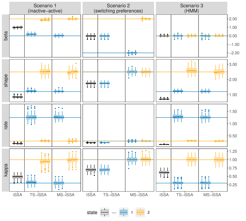
Figure 3: Boxplots of the parameter estimates across the $100$ simulation runs for each applied method, simulation scenario and number of control locations $M$, respectively. The rows refer to the estimated selection coefficient (beta), the shape and rate of the gamma-distribution for step length and the concentration parameter (kappa) of the von Mises distribution for turning angle, respectively. The columns refer to the three different simulation scenarios. For each method (iSSA, TS-iSSA and MS-iSSA) and state (state 1: blue, state 2: orange, no state differentiation: black), the three adjacent boxplots refer the use of $M=20$, $M=100$ and $M=500$ control locations per used location for the parameter estimation. Note that in Scenario 2, the TS-iSSA is naturally not capable to distinguish between two states as both share the same movement kernel. Thus, there are only results for a single state.

Overall, the number of available steps $M$ only slightly affected the estimation results in this simulation exercise, especially the results for $M=100$ and $M=500$ are very similar (Figure 3). Thus, the results seem to be stable. The MS-iSSA performed very well across all simulation scenarios and did not produce any evident bias even in the extremer Scenarios 2 (“state-switching preferences”) and 3 (‘HMM”; Figure 3, Tables S3 and S4). The TS-iSSA was able to detect two suitable states in both scenarios with state-dependent movement kernels (Scenarios 1 and 3), although there was a small but evident bias for some parameters, for example, for the selection coefficients in scenario 1 ($0.18$ in state $1$, $-0.13$ in state $2$ for $M=500$), and for the shape parameter in scenario 3 ($0.12$ in state $2$ for $M=500$). For Scenario 1 (“active-inactive”), this is also reflected in the rather large percentage of significant selection coefficients across the simulation runs in state 1 ($39-40\%$ at a significance level of $\alpha=0.05$, Table 2), although the true coefficient is equal to zero. Thus, in contrast to the MS-iSSA, the p-values of the TS-iSSA are not reliable in this active-inactive setting.

		Scen. 1		Scen. 2		Scen. 3
model	no. cont.	$\beta_{1}=0$	$\beta_{2}=2$	$\beta_{1}=-2$	$\beta_{2}=2$	$\beta_{1}=0$	$\beta_{2}=0$
iSSA	20	100	–	57	–	16	–
	100	100	–	57	–	17	–
	500	100	–	58	–	17	–
TS-iSSA	20	40	100	58	–	5	6
	100	42	100	57	–	4	6
	500	39	100	57	–	4	5
MS-iSSA	20	2	100	100	100	4	5
	100	3	100	100	100	2	5
	500	1	100	100	100	5	6

Table 2: Percentage of simulation runs in which the selection coefficients are estimated to be significantly different from zero at a significance level of $\alpha=0.05$, for each scenario and fitted model, respectively.

	MS-iSSA
scenario	20	100	500	HMM
1 (active-inactive)	4.05 (0.83)	3.76 (0.82)	3.70 (0.79)	5.93 (1.47)
2 (switching preferences)	2.12 (0.53)	2.00 (0.52)	1.94 (0.50)	49.01 (4.38)
3 (HMM)	2.49 (0.49)	2.42 (0.51)	2.38 (0.55)	2.39 (0.53)

Table 3: Mean missclassification rate with standard deviation in parentheses across the $100$ simulation runs for each scenario and fitted state-switching model, respectively. The missclassification rate is calculated as the percentage of states incorrectly classified using the Viterbi sequence. The lowest missclassification rate for each scenario is highlighted in bold face.

The iSSA is by its nature unable to distinguish between the underlying states and thus, did not recover the true underlying parameters in either scenario. Especially in Scenario 2 (“switching preferences”), the iSSA selection coefficients were estimated close to zero and the associated p-values would misleadingly indicate no selection for or against the landscape feature in $42\%-43\%$ of the simulation runs (Table 2). Note that the TS-iSSA produced similar results to the iSSA in this scenario, since the inherent HMM classification was not able to distinguish between states that share the same movement kernel, and therefore all steps were classified to belong to the same state.

		AIC			BIC
Scenario	no. cont.	iSSA	HMM	MS-iSSA	iSSA	HMM	MS-iSSA
Scen. 1	20	0	0	100	0	0	100
	100	0	0	100	0	0	100
	500	0	0	100	0	0	100
Scen. 2	20	2	0	98	2	0	98
	100	2	0	98	2	0	98
	500	2	0	98	2	0	98
Scen. 3	20	0	88	12	0	100	0
	100	0	91	9	0	100	0
	500	0	86	14	0	100	0

Table 4: Percentage of simulation runs in which the three candidate models are selected by either AIC or BIC for each simulation scenario and number of control points used for model fitting, respectively. The cells belonging to the true underlying model are highlighted using bold face.

For all three simulation scenarios, the MS-iSSA with $M=500$ available steps achieved the lowest missclassification rate (Table 3). As the data in Scenario 3 were simulated from an HMM, the HMM classification was equally accurate in this scenario. Overall, the MS-iSSA clearly outperformed the other candidate models in its estimation and classification performance in all scenarios.

As the TS-iSSA involves an a-priori HMM classification, it does not provide a proper maximum likelihood value. It is therefore not possible to calculate corresponding AIC or BIC values for model selection. Thus, we only considered iSSAs without state-switching, HMMs without selection (fitted to the same case-control data sets) and MS-iSSAs as candidate models to evaluate information-criteria based model selection in this modelling framework. For Scenario 1 and 2, AIC and BIC performed very well and selected the true underlying model in $100$ and $98\%$ of the simulation runs, respectively (Table 4). In Scenario 3 (“HMM”), the AIC tended to select the true HMM model in most of the cases but occasionally selected the more complex MS-iSSA ($9-14\%$ of the runs), while the BIC again selected the correct model in all simulation runs.

Overall, the simulation runs with lower spatial variation in the landscape variable produced similar results (Section S5.3). However, the lower spatial variation reduces the influence of the habitat selection function on space use. Therefore, the variance in the estimates slightly increased, the HMM missclassification rate decreased in Scenario 1 and the MS-iSSA missclassification rate increased in Scenario 2. In the supplementary simulation scenario without state-switching, the MS-iSSA was able to recovered the true underlying values in state 1, but produced unusable estimates in state 2 (Section S5.2).

3.2 Case Study on bank vole interactions

For most bank vole individuals, the MS-iSSA approach could reasonably distinguish between two activity levels. State 1 was always associated to shorter step lengths compared to state 2 which could correspond to a rather inactive behaviour (Figure 4; mean of the estimated gamma distribution for step length ranging from $1.43$ to $7.38$ in state 1, and from $8.13$ to $20.85$ in state 2, respectively). According to the Viterbi decoded state sequences, the “less active” state 1 was occupied between $15.29\%$ and $66.71\%$ of the observed time period (Table S7), except for male 1 in replicate $4$ which spent $96.60\%$ of the time in state 1 according to its decoded state sequence. It is also the individual with the largest estimated mean step length in both states ($7.38$ in state 1, $20.85$ in state 2). Thus, for this male, interpretation must be taken with care. The TS-iSSA provided mostly similar results for the movement kernel and state classification (Figure S10).

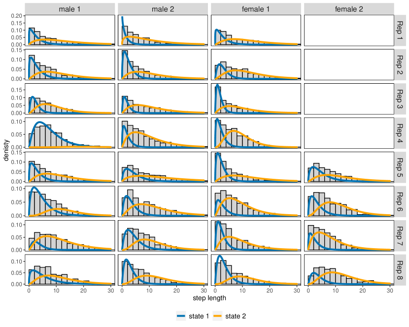
Figure 4: Estimated state-dependent gamma distributions for step length as implied by the fitted $2$-state MS-iSSAs for each individual in replicates $1-8$, respectively. The distributions are weighted by the relative state occupancy frequencies derived from the Viterbi sequence. The gray histograms in the background show the distribution of the observed step lengths.

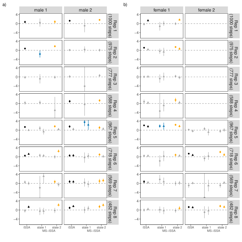
Figure 5: Estimated iSSA and MS-iSSA selection coefficients (solid points/triangles) of interaction behaviour between individuals of opposing sexes within the eight replicates (1–8), including $95\%$ confidence intervals (solid lines). Each replicate consisted of two males (male 1 and male 2) and one or two females (female 1 and female 2) such that each individual could respond to up to two opposite‐sex individuals (dot: response to female/male 1, triangle: response to female/male 2 within a replicate). Non‐significant coefficients (p-values below 0.05) are greyed out. The horizontal dashed line indicates zero (i.e. neutral behaviour); positive coefficients indicate attraction, while negative coefficients would indicate avoidance.

For $21$ of the $28$ bank vole individuals, the MS-iSSA results implied neutral behaviour towards conspecifics in state 1 as all selection coefficients were non-significant ($\alpha=0.05$; Figure 5 and Figure S9). This matches well with the interpretation of a less active/inactive state. For two individuals, the results indicated avoidance behaviour in state 1. In state 2 (“active state”), most bank voles showed attraction to at least one bank vole of opposite sex as implied by the positive and significant selection coefficients. However, for four males and four females, the coefficients for occurrence of individuals with opposite sex were non-significant in both states. These are mainly the individuals for which the iSSA also implied neutral behaviour (Figure 5). However, for 3 individuals, i.e. male 1 in replicate 7, female 1 in replicate 4, and female 1 in replicate 8, the MS-iSSA indicated attraction towards another individual of opposite sex, while the iSSA indicated neutrality. The opposite is true for female 1 in replicate 7 for which only the iSSA indicated attraction. The selection coefficients for occurrence of individuals with same sex usually implied neutral behaviour in state 1, and neutral or attraction behaviour in state 2 (Figure S9).

Overall, the results of the TS-iSSA are in line with the results of the MS-iSSA (Figures S10, S11 and S12), although the implications are slightly different for nine individuals. Regarding information-criteria based model selection, for most bank voles, AIC and BIC pointed to the Markov-switching step-selection model (Table S8). However, for 10 individuals, including half of the female individuals, BIC selected a simpler model, i.e. iSSA or HMM. The selection of HMMs mainly corresponded to cases with many non-significant MS-iSSA selection coefficients. The iSSA was preferred by BIC for male 1 in replicate $4$ and female 2 in replicate 8.

4 Discussion

In this paper, we discussed the relationship between iSSA without underlying behavioural states, the two-step approach TS-iSSA and the joint approach MS-iSSA and compared them in both a simulation and a case study. Thereby, we highlighted possible consequences of either ignoring underlying behavioural states or using a prior HMM-based state classification to take them into account. This provides important implications for the practical application of fine-scale habitat selection analyses.

Combining ideas of iSSAs and HMMs in a single model, MS-iSSAs build a convenient modelling framework to study state-dependent movement and habitat selection based on animal movement data (Nicosia et al.,, 2017; Prima et al.,, 2022). This makes a prior state classification unnecessary, which, as demonstrated in the simulation study, could otherwise lead to biased estimates and misleading conclusions (see also Prima et al.,, 2022). In particular, the MS-iSSA accounts for uncertainties in both the latent state and the observation process which allows for further inference, while the TS-iSSA completely ignores the uncertainties in the state decoding. This renders classical p-values of the TS-iSSA invalid.

Moreover, the MS-iSSA can detect states associated to same movement but different selection behaviour (Scenario 2 in the simulation study), which is not possible using a prior classification that ignores the selection patterns. While Scenario 2 (“switching preferences”) might cover a rather extreme case, one could imagine, for example, an underlying hungry and a thirsty state where the animal is searching for either food or water, or an attraction and neutrality/avoidance state where the animal is either attracted to another individual or ignoring/avoiding possible social interactions. Even if the movement patterns might not be completely the same across these states, they might largely overlap and therefore lead to problems and high uncertainties in the prior state decoding of the TS-iSSA. This is contrasted with Scenario 3 (“HMM”) of the simulation study which does not include any habitat selection, the states are solely associated with different movement kernels. Here, an HMM-based classification is suitable and the TS-iSSA and MS-iSSA perform equally well. Still, the TS-iSSA does not propagate the uncertainties of the state-decoding.

Our analyses further demonstrates that ignoring underlying behavioural states completely by using standard iSSA can strongly corrupt results on selection behaviour. While theoretically expected, a systematic evaluation and quantification of this effect had been lacking. Our study shows that iSSA tends to average out different selection behaviours in different behavioural states. This can lead to simple over- or underestimation of selection strength, keeping the overall direction of selection (i.e., avoidance or attraction) correct. However, it can also lead to more serious problems when selection behaviour has opposing directions in different states. In this case, we found that selection was estimated to be non-significant, which would lead to a strongly erroneous biological conclusion. This result corroborates the surmise that small effect sizes or non-significant results in step-selection analyses may in fact be due to underlying behavioural state switching (Schlägel et al.,, 2019) and more generally the caveat that failure to detect an effect does not imply lack of an affect.

MS-iSSAs have successfully been applied to study habitat selection of bison and zebra in encamped and exploratory states (Nicosia et al.,, 2017; Prima et al.,, 2022), to detect the onset of mule deer migration and to evaluate the behavioural response of bison on the presence of wolves (Prima et al.,, 2022). In our case study, we extend the scope of application to fine-scale interactions of simultaneously tracked bank voles. Here, the 2-state MS-iSSA provided a reasonable separation into a rather inactive state mostly associated with neutral behaviour towards the conspecifics, and an active state often associated with attraction behaviour. However, according to the decoded state sequences, the voles spend more time in the active state as expected ($62.73\%$ of the time on average instead of $25.00\%$). For one male bank vole individual, the state-classification within the MS-iSSA was different. Its second state captured only rare observations with large displacement, while the first state accounted for all other observations. Here, the Viterbi sequence assigned over $96\%$ of the observations to state $1$ and the estimated MS-iSSA showed larger mean step lengths in the estimated state-dependent gamma distributions than for all other individuals. Thus, the second state either captured rare events or outlying observations. This demonstrates that similar care is needed when interpreting the MS-iSSA states as for general HMMs in an unsupervised learning context (McClintock et al.,, 2020).

In the active state, we generally expected males to look for females, while females might show different interactions with males depending on the reproductive state (Schlägel et al.,, 2019). For example, females in estrous may actively seek out males to generate mating opportunities away from the nest to lower the risk of infanticide (Eccard et al.,, 2018). In contrast, females that are not in estrous state might show avoidance or neutrality toward males. In line with Schlägel et al., (2019), for the male bank voles, we found either attraction or neutral behaviour toward the females in the active state. This was, however, also the case for the female responses to male occurrences. While this might reflect the true individual interaction patterns, it might also be an artefact of measurement errors or the fence around the enclosures that limited the space use. Furthermore, some selection coefficient estimates had rather large confidence intervals possibly associated to the small number of observations for the rather complex model structure. This also prevented the use of a $3$-state model that might have been able to differentiate between pure foraging and social interaction states.

With behavioural states being unobserved, it is usually unclear whether they manifest themselves in a given empirical data set. In both the bank-vole and simulation study, we therefore considered information criteria to select between the candidate models iSSA, HMM and MS-iSSA. Especially the BIC performed well in our simulation study. For the TS-iSSA, such likelihood-based criteria cannot be applied as there is no proper joint maximum log-likelihood value for the state and observation process. This is another drawback of the two-step approach. Besides indicating if the inclusion of states or the inclusion of the selection function are appropriate for a given application, information criteria could also be used to select between MS-iSSAs with different covariate sets or generally to select an appropriate number of meaningful biological states $N$. In the context of HMMs, however, the latter has proven difficult, as information criteria, especially the AIC, tend to select overly complex models with a rather large number of states (Celeux and Durand,, 2008; Pohle et al.,, 2017). We expect this to be the case also for MS-iSSAs. Therefore, besides information criteria, the selection of the number of states should further be based on a close inspection of the fitted models, and involve expert knowledge (“pragmatic order selection”, Pohle et al.,, 2017). This is also highlighted in the supplementary simulation scenario which does not include state-switching. Furthermore, future research could focus on the development of appropriate model checking methods for (Markov-switching) step-selection models.

It is important to note that the resolution of the data in time and space can strongly influence the model results and interpretation. Data sets with different resolutions might reflect different state, movement and selection patterns of an animal (Mayor et al.,, 2009; Adam et al.,, 2019). For example, an individual can exhibit many behaviours during a long time interval, e.g. during $24$ hours, and thus, a coarse time resolution might hinder the model to detect biological states such as resting and foraging or provide only crude state proxies. However, migration modes might be reflected in the data. On the other hand, movement and selection patterns might not directly be expressed in steps at very fine time resolution, e.g. based on one location every second (Munden et al.,, 2021). Thus, the temporal resolution of the data must match the time scale in which the animal expresses its state, movement and selection patterns of interest. Moreover, if the spatial resolution of a covariate map is too coarse, important habitat features might be overlooked in the analysis (Zeller et al.,, 2017). Thus, the resolution of the data is a key factor in MS-iSSAs. However, once movement and habitat data are available at a suitable resolution in space and time for a given species and research question at hand, the MS-iSSA approach can flexibly be applied to study fine-scale state-dependent movement and habitat selection. To facilitate its use, the basic MS-iSSA is implemented in the R-package msissa available on GitHub (Pohle and Signer,, 2023).

Author contributions

JP, UES and JS conceived the ideas and designed the study. JP implemented the methods with input from UES and JS. JS and JP implemented the R-package. JAE and MD provided the telemetry data and ecological input for the case study. JP led the writing of the manuscript, supported by UES and JS. All authors contributed critically to the drafts and gave final approval for publication.

Data Availability

The bank vole data are available from the Dryad Digital Repository: https ://doi.org/10.5061/
dryad.rt535m8 (Schlägel et al.,, 2019).

References

- Adam et al., (2019) Adam, T., Griffiths, C. A., Leos-Barajas, V., Meese, E. N., Lowe, C. G., Blackwell, P. G., Righton, D., and Langrock, R. (2019). Joint modelling of multi-scale animal movement data using hierarchical hidden Markov models. Methods in Ecology and Evolution, 10(9):1536–1550.
- Avgar et al., (2016) Avgar, T., Potts, J. R., Lewis, M. A., and Boyce, M. S. (2016). Integrated step selection analysis: bridging the gap between resource selection and animal movement. Methods in Ecology and Evolution, 7(5):619–630.
- Burnham and Anderson, (2002) Burnham, K. P. and Anderson, D. R. (2002). Model Selection and Multimodel Inference: A Practical Information-Theoretical Approach. Springer, New York, 2nd edition.
- Celeux and Durand, (2008) Celeux, G. and Durand, J.-B. (2008). Selecting hidden Markov model state number with cross-validated likelihood. Computational Statistics, 23(4):541–564.
- Cervantes et al., (2023) Cervantes, F., Murgatroyd, M., Allan, D. G., Farwig, N., Kemp, R., Krüger, S., Maude, G., Mendelsohn, J., Rösner, S., Schabo, D. G., Tate, G., Wolter, K., and Amar, A. (2023). A utilization distribution for the global population of cape vultures (gyps coprotheres) to guide wind energy development. Ecological Applications, e2809.
- Ditmer et al., (2021) Ditmer, M. A., Stoner, D. C., Francis, C. D., Barber, J. R., Forester, J. D., Choate, D. M., Ironside, K. E., Longshore, K. M., Hersey, K. R., Larsen, R. T., McMillan, B. R., Olson, D. D., Andreasen, A. M., Beckmann, J. P., Holton, P. B., Messmer, T. A., and Carter, N. H. (2021). Artificial nightlight alters the predator–prey dynamics of an apex carnivore. Ecography, 44(2):149–161.
- Eccard et al., (2018) Eccard, J. A., Reil, D., Folkertsma, R., and Schirmer, A. (2018). The scent of infanticide risk? behavioural allocation to current and future reproduction in response to mating opportunity and familiarity with intruder. Behavioral Ecology and Sociobiology, 72:175.
- Fieberg et al., (2021) Fieberg, J., Signer, J., Smith, B., and Avgar, T. (2021). A ‘How to’ guide for interpreting parameters in habitat-selection analyses. Journal of Animal Ecology, 90(5):1027–1043.
- Fleming et al., (2016) Fleming, C. H., Fagan, W. F., Mueller, T., Olson, K. A., Leimgruber, P., and Calabrese, J. M. (2016). Estimating where and how animals travel: An optimal framework for path reconstruction from autocorrelated tracking data. Ecology, 97:576–582.
- Forester et al., (2009) Forester, J. D., Im, H. K., and Rathouz, P. J. (2009). Accounting for animal movement in estimation of resource selection functions: sampling and data analysis. Ecology, 90(12):3554–3565.
- Fortin et al., (2005) Fortin, D., Beyer, H. L., Boyce, M. S., Smith, D. W., Duchesne, T., and Mao, J. S. (2005). Wolves influence elk movements: behavior shapes a trophic cascade in Yellowstone National Park. Ecology, 86(5):1320–1330.
- Guillen et al., (2023) Guillen, R. A., Lindgren, F., Muff, S., Glass, T. W., Breed, G. A., and Schlägel, U. E. (2023). Accounting for unobserved spatial variation in step selection analyses of animal movement via spatial random effects. bioRxiv, 2023.01.17.524368.
- Karelus et al., (2019) Karelus, D. L., McCown, J. W., Scheick, B. K., van de Kerk, M., Bolker, B. M., and Oli, M. K. (2019). Incorporating movement patterns to discern habitat selection: black bears as a case study. Wildlife Research, 46(1):76–88.
- Langrock et al., (2012) Langrock, R., King, R., Matthiopoulos, J., Thomas, L., Fortin, D., and Morales, J. M. (2012). Flexible and practical modeling of animal telemetry data: hidden Markov models and extensions. Ecology, 93(11):2336–2342.
- Mayor et al., (2009) Mayor, S. J., Schneider, D. C., Schaefer, J. A., and Mahoney, S. P. (2009). Habitat selection at multiple scales. Écoscience, 16(2):238–247.
- McClintock et al., (2020) McClintock, B. T., Langrock, R., Gimenez, O., Cam, E., Borchers, D. L., Glennie, R., and Patterson, T. A. (2020). Uncovering ecological state dynamics with hidden Markov models. Ecology Letters, 23(12):1878–1903.
- Mironov, (1990) Mironov, A. D. (1990). Spatial and temporal organization of populations of the bank vole, clethrionomys glareolus. In Tamarin, R. H., Ostfeld, R. S., Pugh, S. R., and Bujalska, G., editors, Social Systems and Population Cycles in Voles, pages 181–192. Birkhäuser Basel, Basel.
- Munden et al., (2021) Munden, R., Börger, L., Wilson, R. P., Redcliffe, J., Brown, R., Garel, M., and Potts, J. R. (2021). Why did the animal turn? Time-varying step selection analysis for inference between observed turning-points in high frequency data. Methods in Ecology and Evolution, 12(5):921–932.
- Nicosia et al., (2017) Nicosia, A., Duchesne, T., Rivest, L.-P., and Fortin, D. (2017). A multi-state conditional logistic regression model for the analysis of animal movement. The Annals of Applied Statistics, 11(3):1537–1560.
- Northrup et al., (2022) Northrup, J. M., Vander Wal, E., Bonar, M., Fieberg, J., Laforge, M. P., Leclerc, M., Prokopenko, C. M., and Gerber, B. D. (2022). Conceptual and methodological advances in habitat-selection modeling: guidelines for ecology and evolution. Ecological Applications, 32(1):e02470.
- Patterson et al., (2017) Patterson, T., Parton, A., Langrock, R., Blackwell, P., Thomas, L., and King, R. (2017). Statistical modelling of individual animal movement: an overview of key methods and a discussion of practical challenges. AStA Adv Stat Anal, 101:399–438.
- Picardi et al., (2022) Picardi, S., Coates, P., Kolar, J., O’Neil, S., Mathews, S., and Dahlgren, D. (2022). Behavioural state-dependent habitat selection and implications for animal translocations. Journal of Applied Ecology, 59(2):624–635.
- Pohle et al., (2017) Pohle, J., Langrock, R., van Beest, F., and Schmidt, N. M. (2017). Selecting the number of states in hidden Markov models: Pragmatic solutions illustrated using animal movement. JABES, 22:270–293.
- Pohle and Signer, (2023) Pohle, J. and Signer, J. (2023). msissa: R package to fit markov-switching integrated step-selection functions. https://github.com/jmsigner/msissa.
- Prima et al., (2022) Prima, M., Duchesne, T., Merkle, J., Chamaillé-Jammes, S., and Fortin, D. (2022). Multi-mode movement decisions across widely ranging behavioral processes. PLoS One, 17(8):e0272538.
- Prokopenko et al., (2017) Prokopenko, C. M., Boyce, M. S., and Avgar, T. (2017). Characterizing wildlife behavioural responses to roads using integrated step selection analysis. Journal of Applied Ecology, 54(2):470–479.
- R Core Team, (2022) R Core Team (2022). R: A Language and Environment for Statistical Computing. R Foundation for Statistical Computing, Vienna, Austria.
- Ribeiro Jr et al., (2022) Ribeiro Jr, P. J., Diggle, P., Christensen, O., Schlather, M., Bivand, R., and Ripley, B. (2022). geoR: Analysis of Geostatistical Data. R package version 1.9-2.
- Roever et al., (2014) Roever, C. L., Beyer, H. L., Chase, M. J., and van Aarde, R. J. (2014). The pitfalls of ignoring behaviour when quantifying habitat selection. Diversity and Distributions, 20(3):322–333.
- Schirmer et al., (2019) Schirmer, A., Herde, A., Eccard, J. A., and Dammhahn, M. (2019). Individuals in space: personality-dependent space use, movement and microhabitat use facilitate individual spatial niche specialization. Oecologia, 189(3).
- Schlägel et al., (2019) Schlägel, U. E., Signer, J., Herde, A., Eden, S., Jeltsch, F., Eccard, J. A., and Dammhahn, M. (2019). Estimating interactions between individuals from concurrent animal movements. Methods in Ecology and Evolution, 10(8):1234–1245.
- Stratmann et al., (2021) Stratmann, T. S. M., Dejid, N., Calabrese, J. M., Fagan, W. F., Fleming, C. H., Olson, K. A., and Mueller, T. (2021). Resource selection of a nomadic ungulate in a dynamic landscape. PLoS ONE, 16(2):e0246809.
- Suraci et al., (2019) Suraci, J. P., Frank, L. G., Oriol-Cotterill, A., Ekwanga, S., Williams, T. M., and Wilmers, C. C. (2019). Behavior-specific habitat selection by african lions may promote their persistence in a human-dominated landscape. Ecology, 100(4):e02644.
- Therneau, (2020) Therneau, T. M. (2020). A Package for Survival Analysis in R. R package version 3.2-7.
- Viterbi, (1967) Viterbi, A. J. (1967). Error bounds for convolutional codes and an asymptotically optimal decoding algorithm. IEEE Transactions on Information Theory, 13:260–269.
- Zeller et al., (2017) Zeller, K. A., McGarigal, K., Cushman, S. A., Beier, P., Vickers, T. W., and Boyce, W. M. (2017). Sensitivity of resource selection and connectivity models to landscape definition. Landscape Ecology, 32(4):835–855.
- Zucchini et al., (2016) Zucchini, W., MacDonald, I. L., and Langrock, R. (2016). Hidden Markov Models for Time Series: An Introduction Using R. Chapman and Hall/CRC, Boca Raton, 2nd edition.