Deep Unfolding for Fast Linear Massive MIMO Precoders under a PA Consumption Model

Abstract

Massive multiple-input multiple-output (MIMO) precoders are typically designed by minimizing the transmit power subject to a quality-of-service (QoS) constraint. However, current sustainability goals incentivize more energy-efficient solutions and thus it is of paramount importance to minimize the consumed power directly. Minimizing the consumed power of the power amplifier (PA), one of the most consuming components, gives rise to a convex, non-differentiable optimization problem, which has been solved in the past using conventional convex solvers. Additionally, this problem can be solved using a proximal gradient descent (PGD) algorithm, which suffers from slow convergence. In this work, in order to overcome the slow convergence, a deep unfolded version of the algorithm is proposed, which can achieve close-to-optimal solutions in only 20 iterations as compared to the 3500 plus iterations needed by the PGD algorithm. Results indicate that the deep unfolding algorithm is three orders of magnitude faster than a conventional convex solver and four orders of magnitude faster than the PGD.

I Introduction

I-A Problem Formulation

Reducing carbon emissions and energy consumption is more than ever a priority, as it is currently put forward by both Europe’s Green Deal [1] and the United Nations Sustainable Development Goals [2]. Nevertheless, the estimated electricity consumption and carbon footprint of the wireless communications sector continues to rise [3]. As such, when looking at the development of 6G, energy-reducing techniques are of the utmost importance. In current 5G networks, massive MIMO is one of the key enablers [4]. Massive MIMO uses clever precoding schemes to spatially multiplex many users, leading to higher spectral efficiency [5]. These precoders are typically obtained by minimizing the transmit power subject to a QoS constraint (e.g., a per-user signal-to-interference-plus-noise ratio (SINR) constraint). However, it is known that the power consumed by the PAs, one of the most consuming components, does not scale linearly with the transmit power [6, 7]. As such, minimizing the PAs consumed power, rather than the transmit power, can lead to significant energy savings[8]. Moreover, [9] and [8] have shown, for single-user and multi-user systems respectively, that this typically leads to sparse solutions in the number of activated antennas. This can further be exploited by deactivating the RF chains of the unused antennas. Additionally, from [9, 8], it is clear that minimizing the consumed power leads to a convex optimization problem, with the objective function being a composite of a convex, differentiable function and a convex, non-differentiable function. In [8], this problem is solved for a multi-user system using convex solvers. However, when aiming at real-time operation, faster algorithms are required. Given the form of the objective function, a proximal gradient descent (PGD)algorithm can be used to find the global optimum. Unfortunately, PGD suffers from slow convergence, requiring many iterations, which makes the use for real-time applications such as precoding difficult. Therefore, in this work, a deep unfolded version of the PGD algorithm is proposed, which drastically speeds up the optimization, delivering close-to-optimal approximations, in only 20 iterations, as compared to the 5000 needed by PGD.

I-B Deep Unfolding

In recent years, algorithm unrolling, also known as deep unfolding, has provided many promising results in signal and image processing [10]. For instance, the technique has been successfully applied in compressed sensing, sparse coding, image denoising, detection and channel decoding in massive MIMO and many more application domains [10, 11, 12]. Deep unfolding makes the connection between iterative algorithms and deep neural networks. In this scheme, each iteration of an iterative algorithm is represented as a layer in a neural network. This is done for a fixed number of layers/iterations to form a neural network of fixed size. Running the neural network emulates the execution of the traditional algorithm for a finite number of iterations. Furthermore, the main benefit over the traditional algorithm is the fact that algorithm-specific parameters are learned, using backpropagation and stochastic gradient descent-based optimization, while for the traditional algorithm these parameters need to be manually tuned. Learning these parameters in each layer/iteration, produces algorithms that are highly optimized for the problem at hand, and can as such provide faster convergence rates [11]. Many precoding problems lead to iterative optimization algorithms. Consequently, some works have proposed the use of deep unfolding to solve these problems. For instance, in [13] a deep unfolding algorithm is proposed to solve the sum-rate maximization problem in multi-user MIMO. Similarly, in [14], a deep unfolding algorithm is proposed that maximizes the sum-rate while being robust against channel estimation errors. Both works consider a transmit power constraint, neglecting the consumed power in their analysis. In this work, we consider the consumed power and minimized it, which results in a power consumption reduction.

I-C Contributions

In this work, the design of a zero-forcing (ZF) precoder under a realistic PA consumption model is studied. Hence, the PAs consumed power is minimized, rather than the transmit power. First, we show that this leads to a convex optimization problem, with a composite objective function consisting of a convex, differentiable and a convex, non-differentiable part. Given the form of this cost function, the problem can be solved using a PGD algorithm. To support real-time operations, a deep unfolded version of the PGD algorithm is proposed. It is shown that this unfolded algorithm converges to close-to-optimal solutions, much faster than the traditional PGD.

Notations: Vectors and matrices are denoted by bold lowercase and bold uppercase letters respectively. Superscripts $(\cdot)^{*}$, $(\cdot)^{\intercal}$ and $(\cdot)^{H}$ stand for the conjugate, transpose, and Hermitian transpose operators respectively. Subscripts $(\cdot)_{m}$ and $(\cdot)_{k}$ denote the antenna and user index. The expectation is denoted by $\mathbb{E}\left\{\cdot\right\}$, while $\boldsymbol{\mathrm{D}}_{\boldsymbol{\mathrm{a}}}=\mathrm{diag}\left(\boldsymbol{\mathrm{a}}\right)$ denotes a diagonal matrix whose diagonal entries are equal to the vector $\boldsymbol{\mathrm{a}}$. The element at location $(i,j)$ in the matrix $\boldsymbol{\mathrm{A}}$ is indicated as $[\boldsymbol{\mathrm{A}}]_{i,j}$. The symbols $\left\lVert\cdot\right\rVert_{1}$, $\left\lVert\cdot\right\rVert_{2}$, $\left\lVert\cdot\right\rVert_{2,1}$ and $\left\lVert\cdot\right\rVert_{F}$ indicate the $L_{1}$, $L_{2}$, $L_{2,1}$ and Frobenius norms, respectively. $\boldsymbol{\mathrm{A}}^{1/2}$ denotes the positive square root of $\boldsymbol{\mathrm{A}}$, namely the only Hermitian positive semidefinite matrix such that $\boldsymbol{\mathrm{A}}=\boldsymbol{\mathrm{A}}^{1/2}\boldsymbol{\mathrm{A}}^{1/2}$.

II System Model

II-A Signal Model

Throughout this work, a massive MIMO base station (BS) is considered, equipped with $M$ transmit antennas and serving $K$ single-antenna users. The precoded symbol vector $\boldsymbol{\mathrm{x}}\in\mathbb{C}^{M\times 1}$ is given by

$$\boldsymbol{\mathrm{x}}=\boldsymbol{\mathrm{W}}^{\intercal}\boldsymbol{\mathrm{s}}$$ (1)

where $\boldsymbol{\mathrm{W}}\in\mathbb{C}^{K\times M}$ is the precoding matrix and $\boldsymbol{\mathrm{s}}\in\mathbb{C}^{K\times 1}$ are the transmit symbols, which are assumed to be zero mean, uncorrelated and have unit power. The received signal $\boldsymbol{\mathrm{r}}\in\mathbb{C}^{K\times 1}$ is then

$$\boldsymbol{\mathrm{r}}=\boldsymbol{\mathrm{H}}\boldsymbol{\mathrm{x}}+\boldsymbol{\mathrm{\nu}}$$ (2)

where $\boldsymbol{\mathrm{H}}\in\mathbb{C}^{K\times M}$ is the channel matrix. The vector $\boldsymbol{\mathrm{\nu}}\in\mathbb{C}^{K\times 1}$ contains complex independently and identically distributed (i.i.d.) additive white Gaussian noise (AWGN) with zero mean and variance $\sigma_{\nu}$.

II-B Power Consumption Model

Given that the transmit symbols are uncorrelated, the transmit power at antenna $m$ is

$$p_{m}=\mathbb{E}\left\{|x_{m}|^{2}\right\}=\sum_{k=0}^{K-1}|w_{k,m}|^{2}$$ (3)

where $x_{m}=[\boldsymbol{\mathrm{x}}]_{m}$ is the precoded symbol at antenna $m$ and $w_{k,m}=[\boldsymbol{\mathrm{W}}]_{k,m}$ is the precoding coefficient at antenna $m$ for user $k$. This gives a total transmit power

$$p_{\mathrm{tx}}=\sum_{m=0}^{M-1}\sum_{k=0}^{K-1}|w_{k,m}|^{2}=\left\lVert\boldsymbol{\mathrm{W}}\right\rVert_{F}^{2}.$$ (4)

When considering a realistic power consumption model, the transmit power does not scale linearly with the consumed power. In other words, the efficiency of the PA is not fixed but varies with the transmit power, i.e., typically the closer the PA operates to saturation, the higher the efficiency [7]. For instance, for class B amplifiers, the efficiency scales with the square root of the transmit power [6, 9]

$$\eta_{m}=\eta_{\mathrm{max}}\sqrt{\frac{p_{m}}{p_{\mathrm{max}}}}$$ (5)

where $\eta_{m}$ is the efficiency of the $m$-th PA, $\eta_{\mathrm{max}}$ is the maximal PA efficiency and $p_{\mathrm{max}}$ is the maximal output power of the PA. The total consumed power by the PAs is then

$$p_{\mathrm{cons}} =\sum_{m=0}^{M-1}\frac{p_{m}}{\eta_{m}}=\underbrace{\frac{\sqrt{p_{\mathrm{max}}}}{\eta_{\mathrm{max}}}}_{=\alpha}\sum_{m=0}^{M-1}\sqrt{p_{m}}$$ (6)

$$=\alpha\sum_{m=0}^{M-1}\sqrt{\sum_{k=1}^{K}|w_{k,m}|^{2}}=\alpha\left\lVert\boldsymbol{\mathrm{W}}\right\rVert_{2,1}.$$

III Problem formulation

Classical precoders such as ZF minimize the transmit power under a QoS constraint (e.g., a per-user SINR constraint) [5]. However, when aiming to reduce the PAs’ consumed power, one should minimize the consumed power given in (6) rather than the transmit power in (4). As such, a ZF precoder under the PA consumption model in (6) can be formulated as

$$\min_{\boldsymbol{\mathrm{W}}} \alpha\left\lVert\boldsymbol{\mathrm{W}}\right\rVert_{2,1}$$ (7)

$$\mathrm{s.t.} \boldsymbol{\mathrm{H}}\boldsymbol{\mathrm{W}}^{\intercal}=\sigma_{\nu}\boldsymbol{\mathrm{D}}_{\boldsymbol{\mathrm{\gamma}}}^{1/2}$$

where $\boldsymbol{\mathrm{D}}_{\boldsymbol{\mathrm{\gamma}}}=\mathrm{diag}\left(\gamma_{0},\dotsc,\gamma_{K-1}\right)$ and $\gamma_{k}$ is the target SINR for user $k$. In this formulation, the consumed power by the PAs is minimized under a SINR constraint per user. The precoder design problem (7) has been analyzed in [8] and can be solved by using convex optimization toolboxes (e.g., CVXPY [15]). Problem (7) is equivalent to

$$\min_{\boldsymbol{\mathrm{W}}} \alpha\left\lVert\boldsymbol{\mathrm{W}}\right\rVert_{2,1}$$ (8)

$$\mathrm{s.t.} \left\lVert\boldsymbol{\mathrm{H}}\boldsymbol{\mathrm{W}}^{\intercal}-\sigma_{\nu}\boldsymbol{\mathrm{D}}_{\boldsymbol{\mathrm{\gamma}}}^{1/2}\right\rVert_{F}^{2}=0.$$

This optimization problem can be reformulated using a Lagrangian function as follows

$$\begin{split}\mathcal{L}&=\alpha\left\|\boldsymbol{\mathrm{W}}\right\|_{2,1}+\mu\left\lVert\boldsymbol{\mathrm{H}}\boldsymbol{\mathrm{W}}^{\intercal}-\sigma_{\nu}\boldsymbol{\mathrm{D}}_{\boldsymbol{\mathrm{\gamma}}}^{1/2}\right\rVert_{F}^{2}\\ &=\mu\left(\lambda\left\|\boldsymbol{\mathrm{W}}\right\|_{2,1}+\left\lVert\boldsymbol{\mathrm{H}}\boldsymbol{\mathrm{W}}^{\intercal}-\sigma_{\nu}\boldsymbol{\mathrm{D}}_{\boldsymbol{\mathrm{\gamma}}}^{1/2}\right\rVert_{F}^{2}\right)\end{split}$$ (9)

where $\lambda=\alpha/\mu$ and $\mu$ is the Lagrange multiplier.

IV Proximal Gradient Descent

The Lagrangian function in (9) is of the form

$$\mathcal{L}=\lambda g(\boldsymbol{\mathrm{W}})+f(\boldsymbol{\mathrm{W}})$$ (10)

with $f(\boldsymbol{\mathrm{W}})$ a convex, differentiable function and $g(\boldsymbol{\mathrm{W}})$ a convex, non-differentiable function. Given this form, the problem can be solved using PGD [16]. This algorithm first performs a gradient update with respect to the differentiable function $f(\boldsymbol{\mathrm{W}})$. Next, the proximal operator of $\lambda g(\boldsymbol{\mathrm{W}})$ is computed on the result of the gradient update. The general formulation of the iterative proximal algorithm is given by

$$\boldsymbol{\mathrm{W}}^{(i+1)}=\mathbf{prox}_{\lambda\eta g}\left(\boldsymbol{\mathrm{W}}^{(i)}-\eta\nabla f(\boldsymbol{\mathrm{W}}^{(i)})\right)$$ (11)

where $\eta$ is the gradient step size and $\mathbf{prox}_{\lambda\eta g}(\cdot)$ is the proximal operator of the function $\lambda g(\cdot)$. Since $\boldsymbol{\mathrm{W}}$ is a complex matrix, $\nabla f(\boldsymbol{\mathrm{W}})$ is defined as $\nabla f(\boldsymbol{\mathrm{W}})=\partial f(\boldsymbol{\mathrm{W}})/\partial\boldsymbol{\mathrm{W}}^{*}=\boldsymbol{\mathrm{W}}\boldsymbol{\mathrm{H}}^{\intercal}\boldsymbol{\mathrm{H}}^{*}-\sigma_{\nu}\boldsymbol{\mathrm{D}}_{\boldsymbol{\mathrm{\gamma}}}^{1/2}\boldsymbol{\mathrm{H}}^{*}$. Additionally, the proximal operator is only defined for real matrices, and consequently the real and imaginary parts of the complex matrix are concatenated in order to produce the following algorithm

$$\boldsymbol{\mathrm{V}}=\boldsymbol{\mathrm{W}}^{(i)}-\eta\left(\boldsymbol{\mathrm{W}}^{(i)}\boldsymbol{\mathrm{H}}^{\intercal}\boldsymbol{\mathrm{H}}^{*}-\sigma_{\nu}\boldsymbol{\mathrm{D}}_{\boldsymbol{\mathrm{\gamma}}}^{1/2}\boldsymbol{\mathrm{H}}^{*}\right)$$ (12)

$$\begin{bmatrix}\boldsymbol{\mathrm{W}}_{\Re}^{(i+1)}\\ \boldsymbol{\mathrm{W}}_{\Im}^{(i+1)}\end{bmatrix}=\mathbf{prox}_{\lambda\eta\left\lVert\cdot\right\rVert_{2,1}}\left(\begin{bmatrix}\boldsymbol{\mathrm{V}}_{\Re}\\ \boldsymbol{\mathrm{V}}_{\Im}\end{bmatrix}\right).$$

Here, $\lambda$ is dependent on the Lagrange multiplier $\mu$ and controls the trade-off between minimizing $g(\boldsymbol{\mathrm{W}})$ and $f(\boldsymbol{\mathrm{W}})$. Furthermore, convergence is guaranteed if the step size for the gradient update is $\eta\leq 1/L$, where $L$ is the Lipschitz constant of $\nabla f(\boldsymbol{\mathrm{W}}^{(i)})$, which is equivalent to an upper bound on the largest eigenvalue of $\boldsymbol{\mathrm{H}}^{\intercal}\boldsymbol{\mathrm{H}}^{*}$ [16].

In order to define the proximal operator of the $L_{2,1}$ norm, we use the fact that the $L_{2,1}$ norm is a separable function, as it can be expressed as the $L_{1}$ norm over the column-wise $L_{2}$ norm. Hence, using the property of proximal operators for separable functions [17], the proximal of the $L_{2,1}$ norm simply becomes a series of $L_{2}$-proximals on each column of $\boldsymbol{\mathrm{W}}$. As such, the proximal operator for column $m$ of $\boldsymbol{\mathrm{W}}$ (denoted as $\boldsymbol{\mathrm{w}}_{m}$) can be expressed as

$$\mathbf{prox}_{\lambda\eta\left\lVert\cdot\right\rVert_{2,1}}(\boldsymbol{\mathrm{w}}_{m}) =\left(1-\frac{\lambda\eta}{\mathrm{max}(\left\lVert\boldsymbol{\mathrm{w}}_{m}\right\rVert_{2},\lambda\eta)}\right)\boldsymbol{\mathrm{w}}_{m}\quad\forall m$$ (13)

$$=\begin{cases}\left(1-\frac{\lambda\eta}{\left\lVert\boldsymbol{\mathrm{w}}_{m}\right\rVert_{2}}\right)\boldsymbol{\mathrm{w}}_{m}&\text{if $\left\lVert\boldsymbol{\mathrm{w}}_{m}\right\rVert_{2}\geq\lambda\eta$}\\ 0&\text{if $\left\lVert\boldsymbol{\mathrm{w}}_{m}\right\rVert_{2}<\lambda\eta$}\end{cases}.$$

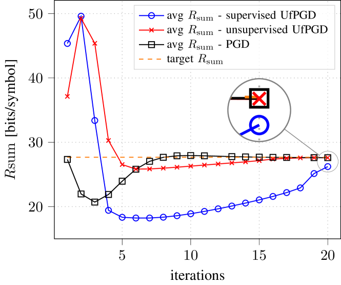
((a)) Average $R_{\mathrm{sum}}$

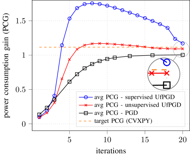
((b)) Average power consumption gain

Figure 1: Sum rate and power consumption gain (PCG)convergence in function of the number of iterations/layers of PGD, unfolding with supervised training and unfolding with unsupervised training. The results are averaged over 5000 channel realizations taken from the test set. Note that the target $R_{\mathrm{sum}}$ and PCG (dashed) are obtained using CVXPY.

V Deep Unfolded Proximal Gradient Descent

The unfolded proximal gradient descent (UfPGD) algorithm follows a similar structure as the algorithm in (12). The algorithm is unrolled for a fixed number of iterations $I$. As such, a neural network consisting of $I$ layers is constructed, with each layer performing the following operations

$$\boldsymbol{\mathrm{V}} =\boldsymbol{\mathrm{W}}^{(i)}-\eta^{(i)}\left(\boldsymbol{\mathrm{W}}^{(i)}\boldsymbol{\mathrm{H}}^{\intercal}\boldsymbol{\mathrm{H}}^{*}-\sigma_{\nu}\boldsymbol{\mathrm{D}}_{\boldsymbol{\mathrm{\gamma}}}^{1/2}\boldsymbol{\mathrm{H}}^{*}\right)$$ (14)

$$\begin{bmatrix}\boldsymbol{\mathrm{W}}_{\Re}^{(i+1)}\\ \boldsymbol{\mathrm{W}}_{\Im}^{(i+1)}\end{bmatrix} =\mathbf{prox}_{\lambda^{(i)}\eta^{(i)}\left\lVert\cdot\right\rVert_{2,1}}\left(\begin{bmatrix}\boldsymbol{\mathrm{V}}_{\Re}\\ \boldsymbol{\mathrm{V}}_{\Im}\end{bmatrix}\right).$$

The key difference between (14) and (12) is the fact that, in the unfolded iteration, the parameters $\lambda^{(i)}$ and $\eta^{(i)}$ are learned parameters that are optimized for each iteration/layer. More specifically, the parameters $\lambda^{(i)}$ and $\eta^{(i)}$ are learned by minimizing a certain cost function $C(\boldsymbol{\mathrm{W}}^{(I)})$, where $\boldsymbol{\mathrm{W}}^{(I)}$ is the output of the neural network (i.e., the result at the $I$-th layer). For instance, this can be done by using stochastic gradient descent in the following manner

$$\lambda^{(i)}_{\mathrm{new}} =\lambda^{(i)}-\beta\frac{\partial C(\boldsymbol{\mathrm{W}}^{(I)})}{\partial\lambda^{(i)}}\quad\forall i\in[1,2,\cdots,I]$$ (15)

$$\eta^{(i)}_{\mathrm{new}} =\eta^{(i)}-\beta\frac{\partial C(\boldsymbol{\mathrm{W}}^{(I)})}{\partial\eta^{(i)}}\quad\forall i\in[1,2,\cdots,I]$$ (16)

where $\partial C(\boldsymbol{\mathrm{W}}^{(I)})/\partial\eta^{(i)}$ and $\partial C(\boldsymbol{\mathrm{W}}^{(I)})/\partial\lambda^{(i)}$ can be computed using backpropagation, and $\beta$ is the learning rate. The cost function can be defined in two ways, namely in a supervised or unsupervised manner. When training in a supervised way, the cost function is simply the mean square error (MSE) between the output of the neural network $\boldsymbol{\mathrm{W}}^{(I)}$ and the known ground truth label for the optimal precoding matrix $\boldsymbol{\mathrm{W}}_{\mathrm{gt}}$

$$C\left(\boldsymbol{\mathrm{W}}^{(I)}\right)=\left\lVert\boldsymbol{\mathrm{W}}^{(I)}-\boldsymbol{\mathrm{W}}_{\mathrm{gt}}\right\rVert_{F}^{2}.$$ (17)

The ground truth labels can be obtained using convex solvers such as CVXPY [15]. When using the supervised learning approach, the MSE acts as a surrogate for the real cost function we want to optimize, which is the Lagrangian in (9). Conversely, one can also train the network in an unsupervised manner by replacing this surrogate loss function with the real cost function which is defined as

$$C\left(\boldsymbol{\mathrm{W}}^{(I)}\right)=\lambda\left\|\boldsymbol{\mathrm{W}}^{(I)}\right\|_{2,1}+\left\lVert\boldsymbol{\mathrm{H}}\left(\boldsymbol{\mathrm{W}}^{(I)}\right)^{\intercal}-\sigma_{\nu}\boldsymbol{\mathrm{D}}_{\boldsymbol{\mathrm{\gamma}}}^{1/2}\right\rVert_{F}^{2}.$$ (18)

Finally, in order to ensure stability during the training, the values of $\lambda^{(i)}$ and $\eta^{(i)}$ are projected into their desired intervals. First, $\lambda^{(i)}$ should be in $[0,+\infty]$, leading to the following projection $\lambda^{(i)}_{\mathrm{projected}}=\max(0,\lambda^{(i)})$. Second, for the classical PGD $\eta^{(i)}=1/L$, where $L$ is an upper bound on the largest eigenvalue of $\boldsymbol{\mathrm{H}}^{\intercal}\boldsymbol{\mathrm{H}}^{*}$. This upper bound can be approximated by the upper limit of the support of the Marchenko-Pastur law, which is (up to scaling) the asymptotic eigenvalue distribution for matrices with i.i.d., zero mean and unit variance entries. This approximation is given by $\tilde{L}=(\sqrt{K}+\sqrt{M})^{2}$ [18]. This bound holds with probability one for sufficiently large $K$ and $M$. Hence, the value of $\eta^{(i)}$ is always projected into the following interval $[1/(2\tilde{L}),1/\tilde{L}]$, where the projection is defined as $\eta^{(i)}_{\mathrm{projected}}=\min(\max(\eta^{(i)},1/(2\tilde{L})),1/\tilde{L})$.

VI Simulations

VI-A Training and Hyperparameters Selection

In this section, simulations are performed to compare the performance of the unfolded and the classical PGD algorithm. For the following simulations, the training set consists of $10^{5}$ Rayleigh fading channels sampled from a complex normal distribution with zero mean and variance one, i.e., $[\boldsymbol{\mathrm{H}}]_{k,m}\sim\mathcal{CN}(0,1)$. The hyperparameters of the unfolding algorithm, such as the learning rate, batch size, etc. were tuned on a validation set of 5000 Rayleigh fading channels. Finally, all simulation results were obtained on an independent test set of 5000 Rayleigh fading channels. For training, the Adam optimizer [19] is used with a batch size of 64 and a learning rate of 0.001. The unfolded algorithm consists of $I=20$ unfolded iterations/layers and was trained for 200 epochs, with early stopping if the validation loss did not further decrease.

VI-B Performance Evaluation Metrics

To compare the performance of the unfolded and classical algorithms, two metrics are considered. First, the sum rate

$$R_{\mathrm{sum}}=\sum_{k=0}^{K-1}\mathrm{log}_{2}(1+\mathrm{SINR}_{k})$$ (19)

where $\mathrm{SINR}_{k}$ is the SINR of user $k$. Given a per-user SINR constraint of $10\ \mathrm{dB}$ and $K=8$ users, the target sum rate the algorithm should achieve is 27.68 bits/symbol. Second, the power consumption gain (PCG) is defined as

$$\mathrm{PCG}=\frac{p_{\mathrm{cons}}^{\mathrm{ZF}}}{p_{\mathrm{cons}}^{\mathrm{ZF-eff}}}$$ (20)

where $p_{\mathrm{cons}}^{\mathrm{ZF}}$ is the consumed power of the ZF precoder, and $p_{\mathrm{cons}}^{\mathrm{ZF-eff}}$ is the consumed power of the proposed power efficient precoder (7), the consumed power is computed using (6).

VI-C Simulation Results

To compare the convergence of PGD and UfPGD, the sum rate and PCG are evaluated at each iteration/layer. This is done for $K=8,M=64$, a target per-user SINR of $\gamma_{k}=10$ $\text{\,}\mathrm{dB}$ and a noise variance of $\sigma_{\nu}=1$. Note that $\lambda=1/15$ for both the PGD algorithm and the unsupervised cost function. Additionally, both PGD and UfPGD are initialized with the conjugate of the channel, i.e., $\boldsymbol{\mathrm{W}}^{(0)}=\boldsymbol{\mathrm{H}}^{*}$.

In Fig. 1(a), the sum rate per iteration is plotted for PGD and UfPGD with supervised and unsupervised training. From this figure it is clear that both PGD and UfPGD with unsupervised training can achieve the target sum rate of 27.68 bits/symbol. When training in a supervised manner, the unfolded algorithm is not able to achieve the goal sum rate. Given that for supervised training the MSE acts as a surrogate for the actual loss function, it is not able to capture the importance of achieving the SINR constraint. When using unsupervised training, the real objective function is optimized, which enables the algorithm to achieve the SINR constraint.

In Fig. 1(b), the PCG per iteration is plotted for PGD and UfPGD. This figure shows that after 20 iterations, the PGD algorithm reaches a PCG of approximately one, indicating that it consumes the same amount of energy as the classical ZF precoder. It is widely known that PGD suffers from slow convergence, as is illustrated in Fig. 2, where the PCG is depicted when the algorithm is run for more iterations. Indeed, from this figure, it is clear that PGD does eventually reach the target PCG. However, it needs over 3500 iterations to get close to the optimal solution. This highlights the benefit of using the unfolded algorithm, as after 20 iterations it is close to the optimal solution. This is depicted in Fig. 1(b), where after 20 iterations the unsupervised UfPGD algorithm reaches a $\mathrm{PCG}=1.0915$, where the target value (obtained with CVXPY) is $\mathrm{PCG}=1.1160$.

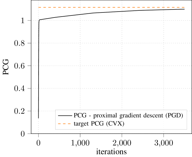
Figure 2: Power consumption gain (PCG)per iteration of PGD, versus the target PCG of CVXPY. Averaged over 5000 channel realizations.

When comparing the execution time of UfPGD, PGD and CVXPY in Fig. 3, it is clear that the unfolding algorithm has the smallest execution time. This is expected as the unfolding algorithm only needs 20 iterations compared to the 5000 needed by PGD. Additionally, it is clear that general-purpose numerical solvers such as CVXPY cannot reach sufficiently low execution times, as the execution times are three orders of magnitude larger than the unfolding algorithm.

VII Conclusion

In this work, a fast unfolded optimization algorithm is developed, for a massive MIMO precoder that minimizes the consumed power rather than the transmit power. It is shown that the optimization problem gives rise to an objective function that consists of a convex, differentiable and a convex, non-differentiable part. Given this form, the optimization problem is solved using PGD. However, given the slow convergence rate of the PGD algorithm, a deep unfolded version of the algorithm is proposed. The proposed algorithm is highly optimized for the task at hand, which allows it to achieve close-to-optimal solutions in only 20 iterations, as compared to the 3500 plus iterations needed by the PGD algorithm. Finally, the execution time of the proposed algorithm is compared against a conventional numerical convex solver (CVXPY), showing that the proposed algorithm is three orders of magnitude faster.

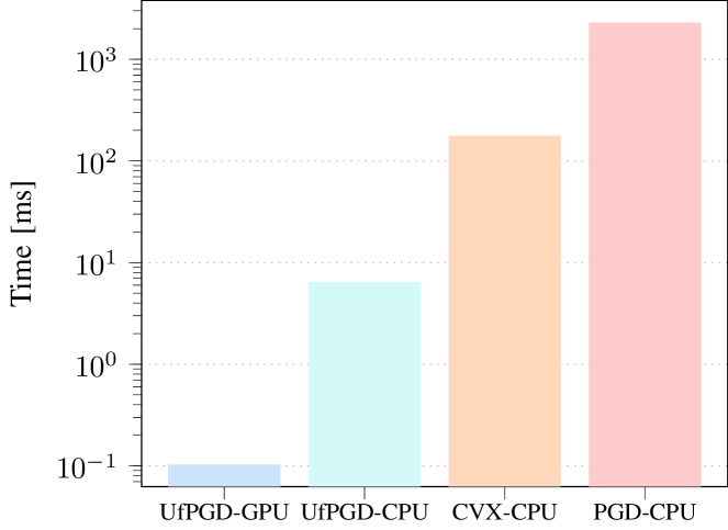
Figure 3: Execution time of UfPGD on GPU and CPU, CVX and PGD, both on CPU (ran for 5000 iterations per execution). Averaged over 5000 executions.

References

- [1] European Commission, “The European Green Deal,” COM (2019), November 2019.
- [2] United Nations, “The 2030 Agenda and the Sustainable Development Goals: An opportunity for Latin America and the Caribbean,” (LC/G.2681-P/Rev.3), Santiago, 2018.
- [3] L. Belkhir and A. Elmeligi, “Assessing ICT global emissions footprint: Trends to 2040 & recommendations,” Journal of Cleaner Production, vol. 177, pp. 448–463, Mar. 2018.
- [4] E. Björnson, L. Sanguinetti, H. Wymeersch, J. Hoydis, and T. L. Marzetta, “Massive mimo is a reality—what is next?: Five promising research directions for antenna arrays,” Digital Signal Processing, vol. 94, pp. 3–20, 2019, special Issue on Source Localization in Massive MIMO.
- [5] E. Björnson, J. Hoydis, and L. Sanguinetti, “Massive MIMO networks: Spectral, energy, and hardware efficiency,” Foundations and Trends® in Signal Processing, vol. 11, no. 3-4, pp. 154–655, 2017.
- [6] A. Grebennikov, RF and Microwave Power Amplifier Design, 1st ed. NY, USA: McGraw-Hill, 2005.
- [7] S. Mikami, T. Takeuchi, H. Kawaguchi, C. Ohta, and M. Yoshimoto, “An Efficiency Degradation Model of Power Amplifier and the Impact against Transmission Power Control for Wireless Sensor Networks,” in 2007 IEEE Radio and Wireless Symposium, 2007, pp. 447–450.
- [8] E. Peschiera and F. Rottenberg, “Linear Precoder Design in Massive MIMO under Realistic Power Amplifier Consumption Constraint,” in 42nd WIC Symposium on Information Theory and Signal Processing in the Benelux, 2022.
- [9] H. V. Cheng, D. Persson, and E. G. Larsson, “Optimal MIMO Precoding Under a Constraint on the Amplifier Power Consumption,” IEEE Transactions on Communications, vol. 67, no. 1, pp. 218–229, 2019.
- [10] V. Monga, Y. Li, and Y. C. Eldar, “Algorithm unrolling: Interpretable, efficient deep learning for signal and image processing,” IEEE Signal Processing Magazine, vol. 38, no. 2, pp. 18–44, 2021.
- [11] K. Gregor and Y. LeCun, “Learning fast approximations of sparse coding,” in Proceedings of the 27th International Conference on International Conference on Machine Learning, ser. ICML’10. Madison, WI, USA: Omnipress, 2010, p. 399–406.
- [12] A. Balatsoukas-Stimming and C. Studer, “Deep unfolding for communications systems: A survey and some new directions,” 2019. [Online]. Available: https://arxiv.org/abs/1906.05774
- [13] Q. Hu, Y. Cai, Q. Shi, K. Xu, G. Yu, and Z. Ding, “Iterative algorithm induced deep-unfolding neural networks: Precoding design for multiuser mimo systems,” IEEE Transactions on Wireless Communications, vol. 20, no. 2, pp. 1394–1410, 2021.
- [14] J. Xu, C. Kang, J. Xue, and Y. Zhang, “A fast deep unfolding learning framework for robust mu-mimo downlink precoding,” IEEE Transactions on Cognitive Communications and Networking, pp. 1–1, 2023.
- [15] S. Diamond and S. Boyd, “CVXPY: A Python-embedded modeling language for convex optimization,” J. Mach. Learn. Res., vol. 17, no. 83, pp. 1–5, 2016.
- [16] F. Bach, R. Jenatton, J. Mairal, and G. Obozinski, “Optimization with Sparsity-Inducing Penalties,” 2011. [Online]. Available: https://arxiv.org/abs/1108.0775
- [17] N. Parikh and S. Boyd, “Proximal Algorithms,” Found. Trends Optim., vol. 1, no. 3, p. 127–239, jan 2014. [Online]. Available: https://doi.org/10.1561/2400000003
- [18] V. A. Marc̃enko and L. A. Pastur, “Distribution of eigenvalues for some sets of random matrices,” Mathematics of The Ussr-sbornik, vol. 1, pp. 457–483, 1967.
- [19] D. P. Kingma and J. Ba, “Adam: A method for stochastic optimization,” 2014. [Online]. Available: https://arxiv.org/abs/1412.6980