The cosmological frame principle and cosmic acceleration

Abstract

We discuss implications of the cosmological frame principle which states that cosmological effects of modified gravity must be stable as solutions of each of the corresponding sets of dynamical equations holding in the two conformally-related frames. We show that there are such globally stable, ‘frame-independent’ solutions describing cosmic acceleration, suggesting that they may represent a physically relevant effect. This result highlights the importance of further investigation into the implications of the frame principle for cosmological properties that rely on the use of conformal frames.

1 Introduction

Modified gravity has become an essential part of theoretical cosmology as an extension of general relativity to understand the nature of gravitational effects in the very early and very late universe, see e.g., [1] - [4] for recent reviews. The conformal potential approach to modified gravity casts the theory in an alternative form by performing a conformal transformation of the original field equations in the Jordan frame to the conformally related Einstein frame representation of the theory as general relativity plus a self-interacting scalar field [5, 6]. This was first introduced for the Brans-Dicke theory [7] by Dicke in [8], for the $f(R)$ gravity theory of [9] in [10], and for the scalar-tensor extension in [11]; for recent investigations cf. [12]-[17].

As is very common in the literature of this vast subject, using the conformal frames one may work at will or choice in any of the two conformally-related theories. In particular, one suspects that even if cosmological phenomena may look different in the two conformally related frames, yet relations between observables must be the same (of course, a mathematical equivalence does not imply a physical one), cf. [18]-[20] and related refs. therein. In these references, a procedure of corresponding effects in the two frames is successfully applied to a variety of deep cosmological questions, such as the singularity problem, the isotropization issue in anisotropic models, or the problem of matching solutions before and after a singularity ‘crossing’. These interesting analyses suggest that one may use the two frames in a productive way to treat cosmological problems through field reparametrization in a similar way as when we have different coordinates systems in classical mechanics. These analyses imply that conformal frames are more than just a mathematical procedure, and possibly suggest the existence of some yet-unknown underlying physical effect taking place between the two conformal frames.

In this paper, we suggest a more precise formulation of this effect which we coin the cosmological frame principle, with the following formulation:

The cosmological frame principle: All cosmological solutions of modified gravity are frame-independent, that is they should preserve their stability properties as solutions of the two conformally-related sets of dynamical equations in the two frames.

The notion of stability in this statement requires some discussion. We mean stability in any given well-defined, mathematical sense, that is Liapunov, asymptotic, orbital, asymptotic orbital, or structural stability of the two systems (or its generalization to system families). Under the frame principle, we propose to accept as a physical effect one that proves stable in any one of the above ways. Therefore a way to test the frame principle in concrete situations is to check the stability of solutions describing the same property in both frames (in the case of structural stability of families, testing the frame principle would imply a full bifurcation analysis of the two systems). If a particular property is proven to be stable as a solution of the equations in some way in both frames (that is for both systems of conformally-related dynamical equations), then it can be regarded as frame-independent in the sense that it exists independently from which frame one uses to study it, despite if it appears differently in the two frames. (It is important to emphasize the use of stable solutions of the two sets of conformally-related dynamical equations in the statement of the frame principle, not just arbitrary functions connected by the conformal transformation between the two frames.)

A prime example is inflation in various contexts (cf. [21] and also [10, 11, 18]), or various cosmic no-hair theorems which give conditions under which de Sitter or quasi-de Sitter spaces are stable in both the $f(R)$ and the Einstein frames, cf. [9, 22, 23, 24, 25], and also the stability of more general Friedmann–Lemaître–Robertson–Walker (FLRW) solutions in both frames [9, 26]. Another example is the viability of an $f\left(R\right)$ theory, for instance, $f(R)=R-\mu^{2(n+1)}/R^{n}$, with $\mu>0,n>1$, promoted to explain the late-time cosmic acceleration [27, 28], for which in the Einstein frame for FLRW models, it was shown in [29] that in the limit $n\rightarrow\infty$, these models are not cosmologically viable. This fact reinforces a general feeling that models with $f(R)=R-\mathrm{const}/R^{n}$ are cosmologically unacceptable [30]. We note that it would be an interesting result if one could show the stability of the matching solutions found in [19, 20] and related references therein, that is show the validity of the cosmological frame principle in the singularity crossing problem.

In this paper, we provide a further example of the use of the frame principle in cosmology, namely, the independence of the property of future acceleration on the choice of frame. We study cosmic acceleration using the frame principle as a guide, and stability analysis in both the Jordan and Einstein frames for flat FLRW universes in the setup of a quadratic Lagrangian gravity theory with a cosmological constant. To this end, in the following two sections we investigate the evolution of FLRW flat models in the quadratic theory with a non-zero cosmological constant of the form $R+\epsilon R^{2}-2\Lambda$ firstly in the Jordan frame (next section) and then in the Einstein frame (Section 3). We prove rigorously that acceleration is a stable property in both frames, and comment on the validity of recollapsing universes with a negative cosmological constant independently of the frame chosen. For simplicity we restrict our analysis to vacuum models, and leave for subsequent work the inclusion of a perfect fluid given its further mathematical intricacies. Our stability proof in this paper reinforces the view that future acceleration is a typical property for these models, and it adds to the physical plausibility of dark energy.

2 Acceleration in the Jordan frame

We adopt the metric and curvature conventions of [31], and choose units so that $c=1=8\pi G$. For the quadratic theory, $R+\epsilon R^{2}-2\Lambda$ in a flat FLRW model, the $00$ equation is,

$$H^{2}+2\epsilon\left(RH^{2}+H\dot{R}-\frac{R^{2}}{12}\right)=\frac{\Lambda}{3},$$ (1)

while the evolution equation for $H$ takes the form,

$$\dot{H}=\frac{1}{6}R-2H^{2}.$$ (2)

We shall also make use of the trace equation which reads,

$$\ddot{R}+3H\dot{R}+\frac{1}{6\epsilon}R=\frac{2\Lambda}{3\epsilon}.$$ (3)

With the variables $R\$and $\dot{R}$, equations (3) and (2) constitute a three-dimensional system. In the following we shall assume that $\epsilon>0$. The non-zero constant $\epsilon$ may be used to define dimensionless variables by the rescaling,

$$R=\frac{2}{\epsilon}x_{1},\ \ \dot{R}=\sqrt{\frac{2}{3\epsilon^{3}}}~{}x_{2},\ \ H=\frac{h}{\sqrt{6\epsilon}},\ \ t=\sqrt{6\epsilon}~{}\tau,$$ (4)

and our system becomes,

$$\dot{x}_{1} =x_{2},$$

$$\dot{x}_{2} =-x_{1}-3x_{2}h+\frac{\lambda}{4},$$ (5)

$$\dot{h} =2x_{1}-2h^{2},$$

where the dot denotes differentiation with respect to $\tau$ and $\lambda=8\epsilon\Lambda$. The constraint (1) takes the form,

$$h^{2}+4x_{1}h^{2}+4hx_{2}-4x_{1}^{2}=\lambda/4.$$ (6)

The only feasible equilibrium point of (5) is

$$\mathbf{q}=\left(x_{1}=\lambda/4,x_{2}=0,h=\sqrt{\lambda}/2\right),$$ (7)

and corresponds to a late accelerating universe.

It turns out that all of the eigenvalues of the Jacobian matrix of (5) at $\mathbf{q}$ have negative real parts, therefore $\mathbf{q}$ is locally asymptotically stable and attracts all nearby solutions. In Figure 1, the solutions $x_{1}\left(t\right)$, $x_{2}\left(t\right)$ and $h\left(t\right)$, are shown approaching their limiting values $1/8$, $0$ and $\sqrt{1/2}/2$ respectively.

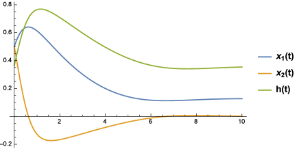
Figure 1: Solutions of (5) for $\lambda=1/2$. The initial values are chosen so that they respect the constraint (6).

3 Acceleration in the Einstein frame

We now consider the quadratic theory $R+\epsilon R^{2}-2\Lambda$ in the conformal frame. The contents of this section follow the path of ideas in [32], but for the sake of completeness we give a brief presentation. The evolution of flat FLRW models is described by the Friedmann equation,

$$H^{2}=\frac{1}{3}\left(\frac{1}{2}\dot{\phi}^{2}+V\left(\phi\right)\right),$$ (8)

the Raychaudhuri equation,

$$\dot{H}=-H^{2}-\frac{1}{3}\dot{\phi}^{2}+\frac{V}{3},$$ (9)

and the equation of motion of the scalar field,

$$\ddot{\phi}+3H\dot{\phi}+V^{\prime}\left(\phi\right)=0.$$ (10)

Here $V\left(\phi\right)$ is the potential energy of the scalar field associated with the conformal transformation and $V^{\prime}=dV/d\phi.$ We assume that the universe is initially expanding, i.e. $H\left(0\right)>0$. Then one can show by standard arguments, [33, 34], that the universe remains ever-expanding, i.e. $H\left(t\right)\geq 0$ for all $t\geq 0$. Using the constraint equation (8), the evolution equation for $H$ simplifies to

$$\dot{H}=-\frac{1}{2}\dot{\phi}^{2}.$$ (11)

Equation (11) implies that $H$ is a decreasing function of time $t$ and is bounded from below either by $0$ or $\sqrt{V(\phi_{\ast})/3})$ where $V^{\prime}(\phi_{\ast})=0$.

For the quadratic theory $R+\epsilon R^{2}-2\Lambda$ the corresponding family of potentials in the Einstein frame is

$$V_{\Lambda}\left(\phi\right)=V_{\infty}\left(1-e^{-\sqrt{2/3}\phi}\right)^{2}+\Lambda e^{-2\sqrt{2/3}\phi},$$ (12)

with $V_{\infty}=1/8\epsilon$. For all $\Lambda>0,$ the functions $V_{\Lambda}\left(\phi\right)$ have a positive minimum $V_{\min}$ at some $\phi_{m}>0$, but otherwise share the same qualitative behaviour as if this term were absent, see Figure 2.

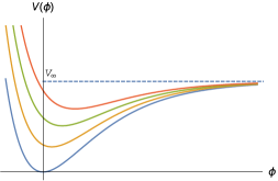
Figure 2: The family of potentials (12) for $V_{\infty}=1$ and $\Lambda$ taking values $0,0.3,0.6,0.9$.

We simplify the system by rescaling the variables as follows,

$$\phi\rightarrow\sqrt{3/2}\,\phi,\ \ \dot{\phi}=\sqrt{2V_{\infty}}\,\,y,\ \ H=\sqrt{\frac{4V_{\infty}}{3}}\,h,\ \ t=\sqrt{\frac{3}{4V_{\infty}}}\,\tau.$$ (13)

Furthermore, in order to take account of the equilibrium point corresponding to the point at “infinity” and to remove the transcendental functions, it is convenient to introduce the variable $u$ defined by,

$$u:=e^{-\phi},$$ (14)

and the system (9)-(10) finally becomes,

$$\dot{u} =-uy,$$

$$\dot{y} =-u+\left(1+\lambda\right)u^{2}-3hy,$$ (15)

$$\dot{h} =-h^{2}-\frac{1}{2}y^{2}+\frac{1}{4}\left(1-u\right)^{2}+\frac{1}{4}\lambda u^{2},$$

where the dot denotes differentiation with respect to $\tau$ and $\lambda=\Lambda/V_{\infty}\equiv 8\epsilon\Lambda$. Note that under the transformation (14), the resulted three-dimensional dynamical system (15) is quadratic. The constraint (8) takes the form

$$h^{2}=\frac{1}{4}\left(y^{2}+\left(1-u\right)^{2}+\lambda u^{2}\right).$$ (16)

In the study of the equilibrium points we note that $u=1$ corresponds to $\phi=0$ and $u=0$ corresponds to $\phi=\infty,$ i.e. to the flat plateau of the potential. There are two equilibrium points of (15):

$$\mathrm{EQ1}:\left(u=0,y=0,h=\frac{1}{2}\right).$$

This corresponds to the de Sitter universe with a cosmological constant equal to $\sqrt{V_{\infty}/3}$, i.e. the scalar field stays at the flat plateau of the potential. A necessary condition for the existence of this equilibrium, is that the scalar field reaches the flat plateau, which is impossible if we restrict ourselves to initial values of $H$ smaller than $\sqrt{V_{\infty}/3}$.

$$\mathrm{EQ2}:\left(u=\frac{1}{\lambda+1},y=0,h=\frac{1}{2}\sqrt{\frac{\lambda}{\lambda+1}}\right).$$ (17)

This corresponds to a late accelerating universe while the scalar field reaches the value $\phi_{m}=\ln\left(1+\lambda\right)$, corresponding to the minimum of the potential.

EQ2 is the most interesting case because, if one could prove that it is stable, this would imply that the late accelerating expansion solution, attracts all nearby solutions. In fact, it is easy to see that the eigenvalues of the Jacobian matrix of (15) at EQ2 are two complex conjugate with negative real parts and one real and negative. Therefore the equilibrium point (17) of (15) is locally asymptotically stable.

In Figure 3, the solutions $u\left(t\right)$, $y\left(t\right)$ and $h\left(t\right)$ approach their limiting values $2/3$, $0$ and $1/\left(2\sqrt{3}\right)$ respectively. These results mean that near the equilibrium EQ2, the dumped oscillations of the scalar field settle down to its minimum value while the Hubble function achieves its constant limiting value $\sqrt{V(\phi_{\min})/3}$.

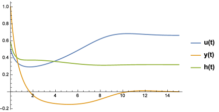
Figure 3: Solutions of (15) for $\lambda=1/2$. The initial values are chosen so that they respect the constraint (16). Note that $u\left(t\right)$ and $y\left(t\right)$ exhibit damped oscillations.

4 Discussion

We have analyzed different aspects of the cosmological frame principle and its possible effects in cosmological settings. In the first Section, we have introduced a new statement of the principle based on possible stability properties of the conformally-related solutions in the two frames. This statement is useful because it provides a practical way to test the possible physical relevance of a cosmological solution of modified gravity.

In Sections 2 and 3 we have shown that cosmic acceleration is a property that respects the frame principle by providing a dynamical systems analysis of the stability of the solutions of quadratic gravity with a cosmological constant in both the Jordan and the Einstein frames. Once one establishes that future acceleration is possible in the Jordan frame, then the frame principle dictates to also expect it in the Einstein frame.

We note that in both frames, late acceleration is provided by the cosmological term, cf. Eqs. (7) and (17). As several authors remark (see for example [30, 35]), $f\left(R\right)$ gravity models can be viable in different contexts. A characteristic example is the $R+\epsilon R^{2}$ theory with the $R^{2}$ term producing an accelerated stage in the early universe preceding the usual radiation and matter stages [21, 22, 23]. A late-time acceleration in this theory (after the matter-dominated stage), however, requires a positive cosmological constant in which case the $R^{2}$ term is no longer responsible for the late-time acceleration.

For $\Lambda<0,$ the potentials (12) have a negative local minimum, hence they belong to the class A of the classification in [36]. Then, although flat, these universes recollapse in the Einstein frame according to Theorem 2 in [36]. We conclude that $\Lambda=0$ in (12) is a bifurcation value for flat models that recollapse or not. Arguments in [21] imply that in the Jordan frame, flat models eventually recollapse as dust-like models with negative $\Lambda$ in general relativity. A firm belief in the frame principle thus allows us to transfer back to the Jordan frame our earlier result valid in the Einstein frame, and therefore confirm the expectation that in the Jordan frame the Starobinsky result complies with our present calculations.

Our formulation of the frame principle as given in this paper allows for a number of known solutions of modified gravity to be tested for stability in the present context in an effort to decide whether or not they preserve their ‘physicality’ when passing between frames. This in principle may be applied not only to cosmology but also to other gravitational frameworks, such as black holes or gravity waves, etc. A more elaborate analysis of these problems necessarily involves the further consideration of structural stability problems associated with the two-conformally-related frames.

References

- [1] S. Capozziello, R. D’Agostino, and O. Luongo, Int. J. Mod. Phys. D 28, No. 10, 1930016 (2019).
- [2] S. Nojiri, S. D. Odintsov and V. K. Oikonomou, Phys. Rep. 692, 1–104, (2017).
- [3] Y. F. Cai, S. Capozziello, M. De Laurentis and E. N. Saridakis, Rept. Prog. Phys. 79 no.4, 106901 (121pp) (2016).
- [4] S. Bahamonde, C. G. Böhmer, S. Carloni, E. J. Copeland, W. Fang and N. Tamanini, Phys. Rep. 775–777, 1–122 (2018).
- [5] S. Cotsakis, I. Klaoudatou, G. Kolionis, J. Miritzis and D. Trachilis, Astronomy 1, 17 (2022); arXiv:2202.06536
- [6] S. Cotsakis and A. P. Yefremov, Phil. Trans. R. Soc. A380 (2022) 20210191 (Part A); ibid., 20210171, (Part B); arXiv:2203.16443
- [7] C. Brans and R. H. Dicke, Phys. Rev. 124, 925 (1961).
- [8] R. H. Dicke, Phys. Rev. 125, 2163 (1962).
- [9] J. D. Barrow and A. C. Ottewill, J. Phys. A 16, 2757 (1983).
- [10] J. D. Barrow and S. Cotsakis, Phys. Lett. B 214, 515 (1988).
- [11] K. I. Maeda, Phys. Rev. D 39, 3159 (1989).
- [12] A. Paliathanasis, Symmetry, 15(2), 529 (2023).
- [13] S. A. Venikoudis, K. V. Fasoulakos, and F. P. Fronimos, Int. J. Mod. Phys. D 31, No. 05, 2250038 (2022).
- [14] S. Capozziello, C. A. Mantica and L. G. Molinari, EPL, 137, 19001 (2022).
- [15] S. Capozziello and G. Lambiase, Eur. Phys. J. Spec. Top. 230, 2123 (2021).
- [16] S. S. Mishra, D. Móller, and A. V. Toporensky Phys. Rev. D 102, 063523 (2020).
- [17] J. D. Barrow and S. Cotsakis, Eur. Phys. J. C 80, 839 (2020).
- [18] Kamenshchik, Alexander Yu., Pozdeeva, Ekaterina O., Tronconi, Alessandro, Venturi. G, Vernov, Sergey Yu., Class.Quant.Grav. 31 (2014) 105003; e-Print: 1312.3540 [hep-th]
- [19] Kamenshchik, Alexander Yu., Pozdeeva, Ekaterina O., Vernov, Sergey Yu., Tronconi, A., Venturi, G., Phys.Rev.D 95 (2017) 8, 083503; e-Print: 1702.02314 [gr-qc]
- [20] Kamenshchik, Alexander Yu., Pozdeeva, E. O., Starobinsky, A. A., Tronconi, A., Venturi, G., Vernov, S. Yu., Phys.Rev.D 97 (2018) 2, 023536; e-Print: 1710.02681 [gr-qc]
- [21] A. A. Starobinsky, Phys. Lett. B 91, 99 (1980).
- [22] A. A. Starobinski, Sov. Astr. Lett. 9, 302 (1983).
- [23] M. B. Mijić, M. S. Morris and W-M. Suen, Phys. Rev. D 34, 2934 (1986).
- [24] S. Cotsakis and G. P. Flessas, Phys. Lett. B 319, 69 (1993).
- [25] S. Cotsakis and J. Miritzis, Class. Quantum. Grav. 15, 2795 (1998).
- [26] S. Cotsakis and G. P. Flessas, Phys. Rev. D 48, 3577 (1993).
- [27] S. Capozziello, V. F. Cardone, S. Carloni and A. Troisi, Int. J. Mod. Phys. D 12, 1969 (2003).
- [28] S. M. Carroll, V. Duvvuri, M. Trodden and M. S. Turner, Phys. Rev. D 70, 043528 (2004).
- [29] K. Tzanni and J. Miritzis, Phys. Rev. D 89, 103540, (2014).
- [30] L. Amendola, R. Gannouji, D. Polarski and S. Tsujikawa, Phys. Rev. D 75, 083504 (2007).
- [31] J. Wainwright and G. F. R. Ellis, Dynamical Systems in Cosmology (CUP, 1997).
- [32] J. Miritzis, J. Math. Phys. 46, 082502 (2005).
- [33] S. Foster, Class. Quantum. Grav. 15, 3485 (1998).
- [34] J. Miritzis, Class. Quantum. Grav. 20, 2981 (2003).
- [35] G. V. Bicknell, J. Phys. A Math. Nucl. Gen. 7, 1061 (1974).
- [36] R. Giambo, J. Miritzis and K. Tzanni, Class. Quantum Grav. 32, 165017 (2015).