Topological properties of a non-Hermitian two-orbital model

Abstract

We perform a thorough analysis of a non-Hermitian (NH) version of a tight binding chain comprising of two orbitals per unit cell. The non-Hermiticity is further bifurcated into $\mathcal{PT}$ symmetric and non-$\mathcal{PT}$ symmetric cases, respectively characterized by non-reciprocal nearest neighbour hopping amplitudes and purely imaginary onsite potential energies. The studies on the localization and the topological properties of our models reveal several intriguing results. For example, they have complex energy gaps with distinct features, that is, a line gap for the non-$\mathcal{PT}$ symmetric case and a point gap for the $\mathcal{PT}$ symmetric case. Further, the NH skin effect, a distinctive feature of the NH system, is non-existent here and is confirmed via computing the local density of states. The bulk-boundary correspondence for both the NH variants obeys a bi-orthogonal condition. Moreover, the localization of the edge modes obtained via the inverse participation ratio shows diverse dependencies on the parameters of the Hamiltonian. Also, the topological properties are discernible from the behaviour of the topological invariant, namely, the complex Berry phase, which shows a sharp transition from a finite value to zero. Interestingly, the $\mathcal{PT}$ symmetric system is found to split between a $\mathcal{PT}$ broken and an unbroken phase depending on the values of the parameters. Finally, the results are benchmarked with the Hermitian model to compare and contrast those obtained for the NH variants.

I Introduction

Energy as a conserved quantity of a quantum mechanical system is ensured by the Hermiticity of the Hamiltonian. On the contrary, when a system is connected to a bath, its interaction with the environment can result in non-Hermitian (NH) dynamics, resulting in markedly distinct behaviour from those of the Hermitian systems. Ever since the pioneering discovery [1] by Bender and Boettcher of NH systems with $\mathcal{PT}$ (parity and time reversal) symmetry exhibiting real energy spectra, these systems have become intriguing subjects for further investigations. Along with the mathematical advances in NH physics [2, 3, 4, 5, 6], recent experimental studies on NH properties in optical systems [7, 8, 9, 10, 11, 12, 13, 14, 15, 16], electronic systems [17, 18, 19, 20, 21], acoustic systems [22, 23, 24, 25, 26, 27] have prompted the exploration of this field in a significant way.

Further, applications of topology in condensed matter physics have started playing a major role in understanding the properties of materials over the last decade or so [28, 29, 30, 31, 32, 33]. Topology is a mathematical field concerned with the study of various types of object geometries. Topology is firmly embedded in the physics of several tight-binding models [32, 33, 34, 35, 36, 37] as they are linked with the properties of the bands. Moreover, the study of materials known as topological insulators (TI) has taken center stage in recent times. They obey certain symmetries, and their topological properties are characterized by different symmetry classes they fall in [38, 30, 31]. The symmetries play a pivotal role in determining the nature of the topological phases. It is possible to define certain physical quantities like winding number [39], Berry phase [40, 41] etc., which remain invariant in these phases, and further change as the system makes a transition from one topological phase to another. The characteristics of these systems undergo substantial modifications when non-Hermiticity is introduced [42, 43, 44, 45, 46, 47, 48, 49], and show exotic behaviors like breaking down of bulk-boundary correspondence (BBC) [48, 50, 51, 52], emergence of exceptional points (EP) [53, 54, 55, 56, 57, 58], complex energy gaps [43, 59, 60], non-Hermitian skin effect (NHSE) [50, 61, 62, 63, 64, 65, 66, 67] etc. These recent studies hint towards the necessity of new fundamental theories for the band topology and localization phenomena of the tight binding systems in the NH platform [68, 48, 50, 69, 70, 71, 72, 60, 73].

There is a particular model that is worth mentioning as it has relevance to the work that we present. One of the two-dimensional (2D) TIs, which shows quantum spin Hall effect (QSHE), is proposed by Bernevig, Hughes, and Zhang (BHZ) [74], which is basically a quantum well (QW), made of HgTe sandwiched between crystals of CdTe, and the corresponding theoretical model in a lattice, a $\mathbb{Z}_{2}$ TI, is proposed by Fu and Kane [75]. They considered a four-band model on a square lattice with each site having two spin half states and two crystal field split $p_{3/2}$ states. A similar model, when considered in one-dimension (1D), albeit simple, may yield intriguing consequences. Further, there have been limited studies on the NH version of the BHZ model [76, 77, 78], where only a term $i\gamma$ is introduced to render non-Hermiticity. A comprehensive investigation of an analog exercise in 1D is still lacking.

In this paper, we present a 1D NH two-band version of the BHZ model consisting of non-interacting spinless fermions, occupying the $s$ and $p_{x}$ orbitals excluding $p_{x}+ip_{y}$ and $p_{x}-ip_{y}$ of the original BHZ model. The onsite energies on the orbitals and the interaction between different orbitals through hopping strengths have been taken into account. To benchmark our results arising from non-Hermiticity, we study the Hermitian model first. We investigate edge states in an open boundary condition (OBC) scenario with both the time reversal symmetry (TRS) and the particle hole symmetry (PHS) remaining intact and compute the Berry phase in periodic boundary conditions (PBC). Hence we include non-Hermiticity into the system in two different ways, namely, by incorporating a staggered onsite imaginary potential ($\mathcal{PT}$ symmetric) and the non-reciprocal hopping amplitudes (non-$\mathcal{PT}$ symmetric). These cases lead to the breaking of time-reversal symmetry (TRS) and sub-lattice symmetry (SLS), respectively. We calculate the complex Berry phase (CBP) [79, 80, 81], and identify the EPs of the system for both scenarios. Furthermore, we demonstrate that there is a profound connection between the complex energy gaps and the presence of EPs. Additionally, we find that the bi-orthogonal BBC (explained later) is preserved, with no indication of NHSE observed in both systems.

Our paper is organized as follows. In section II, we thoroughly examine the Hamiltonians with a view to understanding symmetries and note the symmetry classes to which they belong. In section III, we discuss the results obtained from the individual models in a systematic and sequential manner, that is, discussing the Hermitian case, followed by the non-$\mathcal{PT}$ symmetric and $\mathcal{PT}$ symmetric cases. We plot the (complex) energy spectra for these cases and show the localization of the edge states by computing the inverse participation ratio (IPR) for a finite lattice with OBC. In the presence of PBC, we reveal that the topological invariant, namely the Berry phase for the Hermitian case and CBP for the NH models, assumes either a value of $0$ or $-\pi$, depending on the trivial or the topological phase that the system is in and hence indicates the preservation of the bi-orthogonal BBC via correctly predicting the (dis)appearance of the absolute zero energy edge modes. In section IV, we summarize the results.

II Model Hamiltonians and symmetries

We begin by discussing a simple two-orbital tight-binding model comprising of $s$ and $p_{x}$ orbitals in a unit cell in 1D. The Hamiltonian of the system is given by,

$$H_{0}=\sum_{i=1}^{L}\bigg{[}\epsilon_{s}\hat{s}_{i}^{\dagger}\hat{s}_{i}+\epsilon_{p}\hat{p}_{i}^{\dagger}\hat{p}_{i}- t_{ps}\hat{s}_{i}^{\dagger}\hat{p}_{i-1}\bigg{]}+\sum_{i=1}^{L-1}\bigg{[}-t_{s}\hat{s}_{i}^{\dagger}\hat{s}_{i+1}$$

$$+t_{p} \hat{p}_{i}^{\dagger}\hat{p}_{i+1}+t_{ps}\hat{s}_{i}^{\dagger}\hat{p}_{i+1}\bigg{]}+\textrm{H.c.},$$ (1)

where $\epsilon_{s}$ and $\epsilon_{p}$ are the onsite potentials corresponding to the $s$ and $p_{x}$ orbitals, $-t_{s}$($t_{p}$) and $t_{ps}$($-t_{ps}$) being the hopping strengths for $s^{i-1}\leftrightarrow s^{i}$($p_{x}^{i-1}\leftrightarrow p_{x}^{i}$) and $s^{i-1}\leftrightarrow p_{x}^{i}$($p_{x}^{i-1}\leftrightarrow s^{i}$), respectively (double-headed arrows denote the Hermitian case). $s^{i}$ and $p_{x}^{i}$ suggest $s$ and $p_{x}$ orbitals at $i^{\mathrm{th}}$ unit cell respectively and $L$ denotes the total number of unit cells. $\hat{s}_{i}$($\hat{s}_{i}^{\dagger}$) and $\hat{p}_{i}$($\hat{p}_{i}^{\dagger}$) are annihilation(creation) operators for spinless fermions pertaining to the $s$ and $p_{x}$ orbitals of the $i^{\mathrm{th}}$ unit cell respectively. There is no intra-orbital hopping; that is, hopping amplitude between $s$ and $p_{x}$ orbitals within the same unit cell is neglected. Under PBC, the Hamiltonian in Eq.(1) can be written in the following Bloch form in momentum space as,

$$H_{0}(k)=\frac{1}{L}\sum_{k=1}^{L}\begin{pmatrix}\hat{s}_{k}^{\dagger}&\hat{p}_{k}^{\dagger}\end{pmatrix}h(k)\begin{pmatrix}\hat{s}_{k}\\ \hat{p}_{k}\end{pmatrix},$$ (2)

where $\hat{s}_{k}$($\hat{s}_{k}^{\dagger}$) and $\hat{p}_{k}$($\hat{p}_{k}^{\dagger}$) denote the annihilation(creation) operators in momentum space corresponding to $\hat{s}_{i}$($\hat{s}_{i}^{\dagger}$) and $p_{i}$($p_{i}^{\dagger}$) with $h_{0}(k)$ being the Bloch Hamiltonian which has a form,

$$h_{0}(k)=\begin{pmatrix}\epsilon_{s}-t_{s}e^{-ik}-t_{s}^{*}e^{ik}&2it_{ps}\sin k\\ -2it_{sp}\sin k&\epsilon_{p}+t_{p}e^{-ik}+t_{p}^{*}e^{ik}\end{pmatrix}.$$ (3)

To facilitate a structured discussion, we shall consider three special cases of this model in the following section.

II.1 Hermitian Model

Before going to the NH versions of the system described by Eq.(1), first, we need to understand the properties of the Hermitian counterpart. For this, we shall study a special case of this Hamiltonian by setting $\epsilon_{s}=-\epsilon_{p}=\epsilon$ and $t_{s}=t_{p}=t_{s}^{*}=t_{p}^{*}=t$. With this simplification, the model Hamiltonian in real space can be written as,

$$H_{1} =\sum_{i=1}^{L}\bigg{[}\epsilon(\hat{s}_{i}^{\dagger}\hat{s}_{i}-\hat{p}_{i}^{\dagger}\hat{p}_{i})-t_{ps}\hat{s}_{i}^{\dagger}\hat{p}_{i-1}\bigg{]}+$$

$$\sum_{i=1}^{L-1}\bigg{[}-t(\hat{s}_{i}^{\dagger}\hat{s}_{i+1}-\hat{p}_{i}^{\dagger}\hat{p}_{i+1})+t_{ps}\hat{s}_{i}^{\dagger}\hat{p}_{i+1}\bigg{]}+\textrm{H.c.}$$ (4)

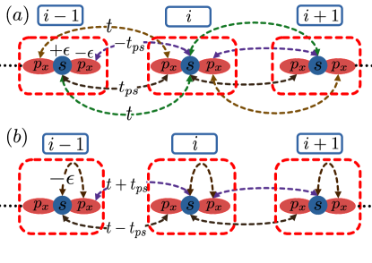
Figure 1: Pictorial representations of (a) the model represented by the Hamiltonian $H_{1}$ (Eq.(4)) (b) the model represented by the Bloch Hamiltonian $h^{\prime}_{1}(k)$ (Eq.(16)). The orbitals, $s$ and $p_{x}$, the hopping amplitudes ($t$ and $t_{ps}$) and the onsite energy ($\epsilon$) are shown.

Fourier transforming Eq.(4), the Bloch Hamiltonian takes the form (Eq.(2)),

$$h_{1}(k)=\begin{pmatrix}\epsilon-2t\cos k&2it_{ps}\sin k\\ -2it_{sp}\sin k&-\epsilon+2t\cos k\end{pmatrix}.$$ (5)

This implies a staggered potential of strength $\epsilon$ at each of the orbitals $s$ and $p_{x}$, hopping amplitudes of $t$ and $t_{ps}$ along $p_{x}^{i}\leftrightarrow p_{x}^{i+1}$ and $s^{i}\leftrightarrow p_{x}^{i+1}$ respectively (see Fig.1(a)). It is well known that the topological phases and localization properties depend on the various symmetries of the system, which can be obtained by observing whether the corresponding symmetry operators commute (or anti-commute) with the Bloch Hamiltonian [82]. In the present case, the system has TRS, which is given by the following relation for any $h(k)$ [83],

$$\mathcal{T}h(k)\mathcal{T}^{-1}=h(-k);\quad\mathrm{with}\quad\mathcal{T}^{2}=\pm 1,$$ (6)

where $\mathcal{T}$ ($=U_{T}\mathcal{K}$, $U_{T}$ being a unitary matrix) is the TRS operator that is anti-unitary in nature, and $h_{1}(k)$ satisfies the above equation. For systems consisting of spinless fermions (present case), $\mathcal{T}$ is nothing but the complex conjugation operator $\mathcal{K}$ and $\mathcal{T}^{2}=1$. This implies that if the Hamiltonian $H_{1}$($h_{1}(k)$) has an eigenvalue $E$($E_{k}$) corresponding to the eigenvector $\ket{\psi}$($\ket{\psi(k)}$), then there also exists an eigenvalue $E^{*}$($E_{-k}^{*}$) corresponding to the eigenvector $\ket{\psi}^{*}$($\ket{\psi(-k)}^{*}$). In the same way, the system also possesses PHS, which is written as,

$$\mathcal{C}h(k)\mathcal{C}^{-1}=-h(-k);\quad\mathrm{with}\quad\mathcal{C}^{2}=\pm 1.$$ (7)

The anti-unitary PHS operator $\mathcal{C}=U_{C}\mathcal{K}$ ($U_{C}$ is unitary) anti-commutes with the Bloch Hamiltonian $h_{1}(k)$, where $U_{C}=\sigma_{x}$ for the present case. Thus, the eigenvalues come in pairs, $\pm E$, with corresponding eigenvectors being $\ket{\psi}$ and $\mathcal{C}\ket{\psi}$. Evidently, the chiral symmetry (CS) is also there since the CS operator ($\Gamma$) is nothing but $\Gamma=\mathcal{T}\cdot\mathcal{C}$. These properties allow us to conclude that the system falls in the class $\pmb{\mathrm{BDI}}$ in $\pmb{\mathrm{AZ}}$ symmetry class [38].

II.2 NH models

Next, we explore the NH extensions of the Hermitian model described by Eq.(4). A well-adapted (and usually employed) way to convert a Hermitian model to an NH one can be done via,

1. introducing imaginary onsite potential (or random disorders).

2. breaking the reciprocity in the hopping strengths between the lattice sites.

II.2.1 Non-$\mathcal{PT}$ symmetric NH Model

Here we only introduce a staggered imaginary onsite potential to the orbitals of the system. This will result in a Hamiltonian of the form given by,

$$H_{2} =\sum_{i=1}^{N}\bigg{[}i\epsilon(\hat{s}_{i}^{\dagger}\hat{s}_{i}-\hat{p}_{i}^{\dagger}\hat{p}_{i})-t_{ps}\hat{s}_{i}^{\dagger}\hat{p}_{i-1}\bigg{]}+$$

$$\sum_{i=1}^{N-1}\bigg{[}-t(\hat{s}_{i}^{\dagger}\hat{s}_{i+1}-\hat{p}_{i}^{\dagger}\hat{p}_{i+1})+t_{ps}\hat{s}_{i}^{\dagger}\hat{p}_{i+1}\bigg{]}+\textrm{H.c.},$$ (8)

where $\epsilon$ is the magnitude of the imaginary onsite potential. The corresponding Bloch Hamiltonian is given by,

$$h_{2}(k)=\begin{pmatrix}i\epsilon-2t\cos k&2it_{ps}\sin k\\ -2it_{sp}\sin k&-i\epsilon+2t\cos k\end{pmatrix}.$$ (9)

The $i\epsilon$ term will break TRS and hence will not possess $\mathcal{PT}$ (or anti-$\mathcal{PT}$) symmetry, owing to,

$$(\mathcal{PT})h_{2}(k)(\mathcal{PT})^{-1}=-h_{2}^{*}(k)\neq h_{2}(k),$$

where $\mathcal{PT}$ operator is given by $\sigma_{x}\mathcal{K}$. It is known that in NH systems, there exists an $\pmb{\mathrm{AZ}^{\dagger}}$ symmetry class [70], apart from the $\pmb{\mathrm{AZ}}$ symmetry class, since $H^{*}\neq H^{T}$. Thus, this system has another symmetry $\mathrm{TRS}^{\dagger}$ from $\pmb{\mathrm{AZ}^{\dagger}}$ class, which demands,

$$\mathcal{C}_{+}h^{T}(k)\mathcal{C}_{+}^{-1}=h(-k);\quad\mathrm{with}\quad\mathcal{C}_{+}\mathcal{C}_{+}^{*}=\pm 1,$$

with $\mathcal{C}_{+}$ being an unitary matrix, as it satisfies $h_{2}^{T}(k)=h_{2}(-k)$. So, the present model falls in the class $\pmb{\mathrm{D}}$ in the real $\pmb{\mathrm{AZ}}$ symmetry class (due to PHS) with $\mathcal{S_{-}}$ SLS [71] as the SLS operator, which is represented by $\sigma_{z}$ for a bipartite lattice, anti-commutes with PHS operator, $\mathcal{C}$ in Eq.(7). It also falls in the class $\pmb{\mathrm{AI}^{\dagger}}$ in the real $\pmb{\mathrm{AZ}^{\dagger}}$ symmetry class due to $\mathrm{TRS}^{\dagger}$.

II.2.2 $\mathcal{PT}$ symmetric NH model

Now we take recourse to break the Hermiticity of $H_{1}$ by including a non-reciprocity parameter, $\delta$, in the hopping term ($t_{ps}$) among the $s$ and $p_{x}$ orbitals from neighbouring unit cells. The new Hamiltonian in OBC takes the form,

$$H_{3}=H_{1}+\delta\left[\sum_{i=1}^{N-1}(\hat{s}_{i}^{\dagger}\hat{p}_{i+1}-\hat{p}_{i+1}^{\dagger}\hat{s}_{i})-\sum_{i=1}^{N}(\hat{s}_{i}^{\dagger}\hat{p}_{i-1}-\hat{p}_{i-1}^{\dagger}\hat{s}_{i})\right]$$ (10)

with the Bloch Hamiltonian, $h_{3}(k)$, in PBC given by,

$$h_{3}(k)=\begin{pmatrix}\epsilon-2t\cos k&2i(t_{ps}+\delta)\sin k\\ -2i(t_{sp}-\delta)\sin k&-\epsilon+2t\cos k\end{pmatrix}.$$ (11)

which indicates that the forward ($s^{i}\rightarrow p_{x}^{i+1}$) and the backward ($s^{i}\leftarrow p_{x}^{i+1}$) hopping amplitudes between $s^{i}$ and $p_{x}^{i+1}$ is $t_{ps}-\delta$ and $t_{ps}+\delta$, respectively. The non-reciprocity term does not affect the TRS or the PHS of the Hermitian model. Hence, $h_{3}(k)$ satisfies Eqs.(6) and (7), and also has CS, but does not have the SLS. While CS and SLS are the same for the Hermitian system, they are different for NH systems. SLS is given by,

$$\mathcal{S}h(k)\mathcal{S}^{-1}=-h(k);\quad\mathrm{with}\quad\mathcal{S}^{2}=1,$$

where $\mathcal{S}$ denotes a unitary matrix. Thus the system falls in class $\pmb{\mathrm{BDI}}$ in real $\pmb{\mathrm{AZ}}$ symmetry class due to the presence of all three (TRS, PHS, and CS) symmetries. $h_{3}(k)$ also falls in class $\pmb{\mathrm{D}^{\dagger}}$ due to topological unification of TRS and $\textrm{PHS}^{\dagger}$ [84]. Apart from these, the model also has $\mathcal{PT}$ symmetry, which we shall show later.

III Results

In this section, we explore the topological and localization properties of the above three models (Hermitian and two variants of the NH models) with OBC and establish the (bi-orthogonal) BBC with the help of the corresponding topological invariants for each model for PBC. We calculate the IPR, the energy spectra in both real and $k$-space, and the (complex) Berry phase as the topological invariant to extract information on the behaviour of the systems.

III.1 Hermitian model

First, we take the Hermitian model represented by Eq.(4) for a 1D chain of length $L$. In Fig.2(a) we have presented the real space eigenspectra with the onsite energy $\epsilon$ being varied from $0$ to $4t$. Here we have set $t=t_{ps}=1$ and, in most cases, set the energy scale to be in a unit of $t$. The existence of a two-fold degenerate zero energy edge state till $\epsilon=2t$ and their disappearance beyond that point is suggestive of a topological phase transition at that point.

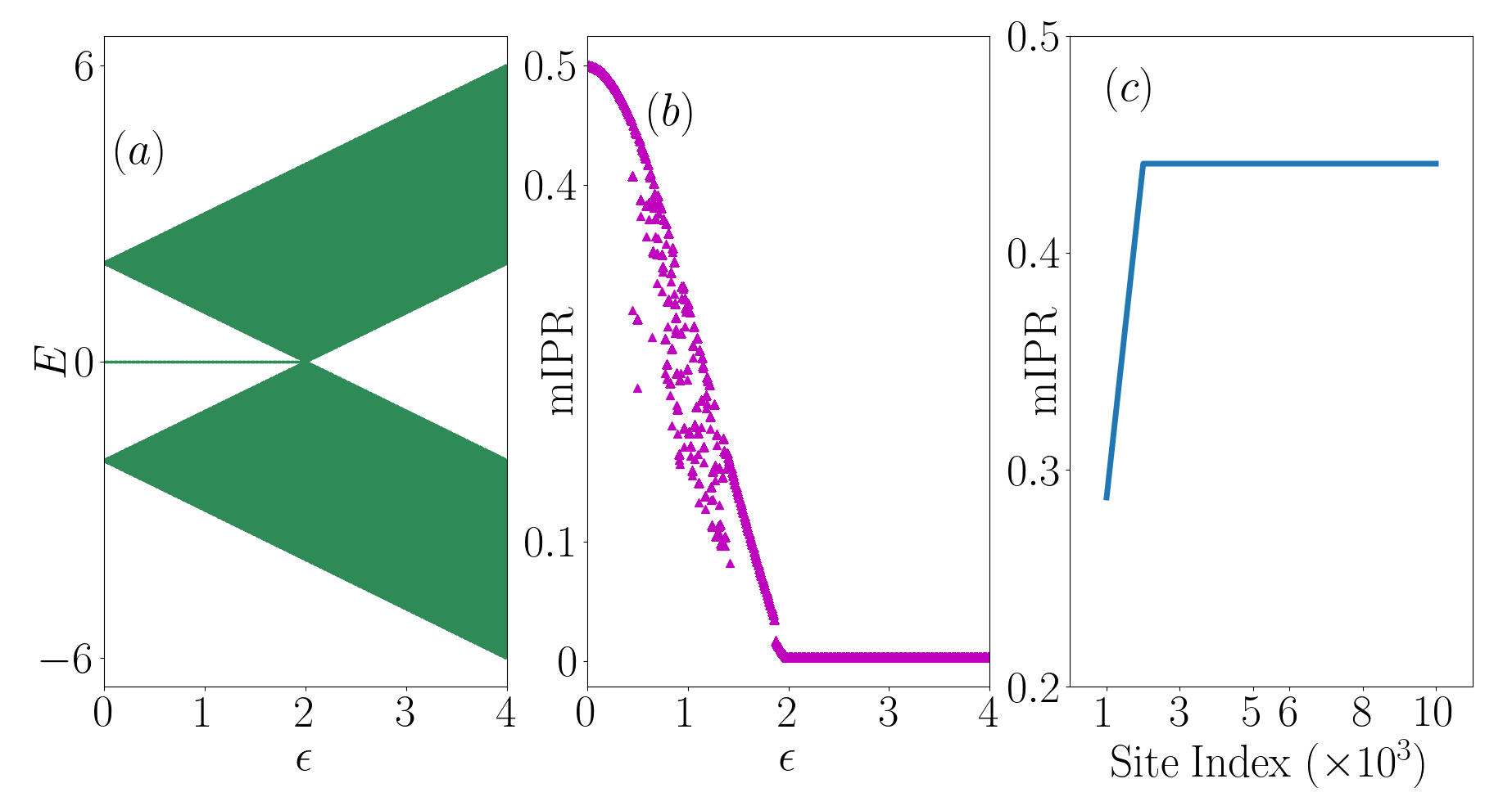
Figure 2: (a) Eigenvalues of $H_{1}$ (Eq.(4)) vs $\epsilon$, showing the appearance(disappearance) of zero energy eigenstates prior to(beyond) $\epsilon=2t$, (b) mIPR vs $\epsilon$ is shown, suggesting that the localization to delocalization phase transition occurs at $\epsilon=2t$, and (c) system size effects on mIPR with $\epsilon=0.5t$. For plots (a) and (b), the system comprises of $1000$ unit cells. The rest of the plots are shown for the same size.

To ascertain the localization of the eigenstates, we use the familiar approach of computing the IPR [85], defined via,

$$\mathrm{IPR}^{(i)}=\frac{\sum_{n}|\psi^{i}_{n}|^{4}}{\left(\sum_{n}|\psi^{i}_{n}|^{2}\right)^{2}},$$ (12)

where $\mathrm{IPR}^{(i)}$ is the IPR of the $i$-th eigenstate and $n$ denotes site index. It is well established that for extended states, the IPR varies inversely with the system size ($\sim L^{-1}$), whereas for the localized states, the IPR become independent of the system size and approaches $1$ (in the thermodynamic limit) when they are completely localized. The maximum IPR (mIPR) represents the IPR of the edge states. Further, it also denotes the highest value of IPR among all the eigenstates for the trivial phase, which does not have edge states. It is being plotted as a function of the potential, $\epsilon$, in Fig.2(b). The non-zero values suggest that the number of the localized eigenstates at the edges are non-zero till the point $\epsilon\leq 2t$ and zero when all the eigenstates are delocalized for $\epsilon>2t$. Fig.2(c) shows the system size effects on mIPR, suggesting that it is independent of the system size beyond a critical system size of $L\sim 1000$. Thus, we have used kept the number of unit cells fixed at $1000$ for all the calculations.

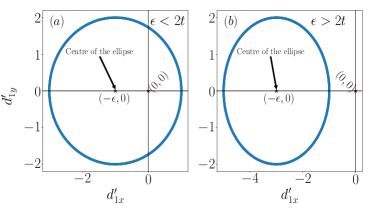
Figure 3: The locus of $\pmb{d^{\prime}_{1}}$-vector (an ellipse) in $d^{\prime}_{1x}-d^{\prime}_{1y}$ plane for the two cases, namely, (a) $\epsilon<2t$, where the origin $(0,0)$ is inside the closed loop, and (b) $\epsilon>2t$, where the origin is outside the ellipse. The center of the ellipse is at (-$\epsilon$,0).

In order to establish BBC, we shall do the calculations in the momentum space (PBC) and compute the values of the topological invariant. $h_{1}(k)$ in Eq.(5) can be written as a Dirac Hamiltonian, $h_{1}(k)=\pmb{d_{1}\cdot\sigma}$, where $\pmb{d_{1}}\equiv(0,-2t_{ps}\sin k,\epsilon-2t\cos k)$ and $\pmb{\sigma}$ denote the Pauli matrices. The $\pmb{d_{1}}$-vector plays a crucial role in understanding the BBC in the following sense. The eigenvalues of $h_{1}(k)$ are given by,

$$E_{\pm}(k)=\pm|\pmb{d_{1}}|=\pm\sqrt{(\epsilon-2t\cos k)^{2}+4t_{ps}^{2}\sin^{2}k}.$$ (13)

We shall perform a unitary transformation on $h_{1}(k)$ to make the $d_{x}$ term non-zero. This is achieved via a unitary matrix $U$, such that,

$$h_{1}^{\prime}(k)=U^{\dagger}h_{1}(k)U;\quad\mathrm{where}$$ (14)

$$U=\frac{1}{\sqrt{2}}\begin{pmatrix}1&-1\\ 1&1\end{pmatrix},$$ (15)

which yields,

$$h_{1}^{\prime}(k)=\begin{pmatrix}0&-\epsilon+2t\cos k\\ &+2it_{ps}\sin k\\ -\epsilon+2t\cos k\\ -2it_{ps}\sin k&0\end{pmatrix},$$ (16)

The transformed Bloch Hamiltonian $h^{\prime}_{1}(k)$ corresponds to a different two-orbital model shown in Fig.1(b), which has $-\epsilon$ and $t+t_{ps}$($t-t_{ps}$) as the hopping amplitudes for $s^{i}\leftrightarrow p_{x}^{i}$ and $p_{x}^{i}\leftrightarrow s^{i+1}$($s^{i}\leftrightarrow p_{x}^{i+1}$) respectively. However, it falls under the same symmetry class, namely $\pmb{\mathrm{BDI}}$, which ensures that it has all the symmetries which the original model (represented by $h_{1}(k)$) possesses. This is obvious because they are connected via a similarity transformation, and hence the band structure remains identical. Hence they must be ‘topologically equivalent’. The expression for $E_{1}(k)$ is given by,

$$E_{1\pm}(k)=\pm\sqrt{(-\epsilon+2t\cos k)^{2}+4t_{ps}^{2}\sin^{2}k},$$ (17)

where the Dirac form for $h^{\prime}_{1}(k)$ is given as, $h^{\prime}_{1}(k)=\pmb{d^{\prime}_{1}\cdot\sigma}$ with $\pmb{d^{\prime}_{1}}\equiv(-\epsilon+2t\cos k,-2t_{ps}\sin k,0)$.

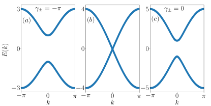
Figure 4: the energy dispersion corresponding to $H_{1}$ shown for the three cases, namely, (a) $\epsilon<2t$ (gapped), (b) $\epsilon=2t$ (where the spectral gap closes), and (c) $\epsilon>2t$ (gap reopens) keeping $t=t_{ps}=1$. (a) and (c) imply the topological and the trivial phases of $H_{1}$, whereas (b) shows a phase transition point.

The unitary transformation interchanges the $x$ and the $z$ components of the $\pmb{d_{1}}$-vector in addition to rendering a negative sign, that is, $d^{\prime}_{1x}=-d_{1z}$ and $d^{\prime}_{1z}=-d_{1x}$. In the $d^{\prime}_{1x}-d^{\prime}_{1y}$ plane, the $\pmb{d^{\prime}_{1}}$-vector forms a loop (see Fig.3) as $k$ goes from $-\pi$ to $+\pi$ in the Brillouin zone (BZ) and includes the origin ($0,0$), which can be thought of as the EP of the system about which the trajectory of the $\pmb{d^{\prime}_{1}}$-vector can be seen to look for the topological properties. For the case $\epsilon<2t$, the EP is enclosed (Fig.3(a)) and excluded (Fig.3(b)) when $\epsilon>2t$. The band structure given by Eq.(17) is plotted in Fig.4. The first column (Fig.4(a)) and the third column (Fig.4(c)) show gapped eigenspectra corresponding to the cases $\epsilon<2t$ and $\epsilon>2t$, respectively, but with different values of Berry phase which we will discuss later in this section. They correspond to the scenario depicted in Fig.3(a) and Fig.3(b), respectively. The spectral gap vanishes at $k=0$ in Fig.4(b), which corresponds to $\epsilon=2t$, which is the case when the EP ($0,0$) lies on the locus of the $\pmb{d^{\prime}_{1}}$-vector.

The BBC implies that some topological invariant must exist, which with aid in extracting information about the edge (OBC) through the information obtained from the bulk (PBC). A useful quantity pertaining to particular topological phases of matter is the Berry phase [41]. It is a geometric phase acquired by the eigenstates over an adiabatic cycle in the parameter space, such as time, position, momentum, etc. We shall use Berry phase as the suitable invariant throughout the paper, whose definition is given by,

$$\gamma_{\pm}=i\oint_{BZ}\bra{\psi_{\pm}(k)}\nabla_{k}\ket{\psi_{\pm}(k)}\;dk,$$ (18)

where $\ket{\psi_{+}(k)}$($\ket{\psi_{-}(k)}$) is the eigenvector corresponding to the upper(lower) band of the Bloch Hamiltonian and $\pm$ signs label the band index. Generally, the Berry phase is an integer (positive or negative) in the unit of $\pi$. In the present case, the eigenvectors of $h^{\prime}_{1}(k)$ corresponding to the eigenvalues $E_{1\pm}(k)$ are given by,

$$\ket{\psi^{\prime}_{1\pm}(k)}=\pm\frac{1}{\sqrt{2}}e^{\pm i\zeta}\begin{pmatrix}e^{-i\phi_{1k}}\\ 1\end{pmatrix},$$ (19)

where $\zeta$ is independent of $k$ and $\phi_{1k}$ is given by,

$$\phi_{1k}=\tan^{-1}\left(\frac{2t_{ps}\sin k}{\epsilon-2t\cos k}\right).$$ (20)

Putting $\ket{\psi^{\prime}_{1\pm}(k)}$ in Eq.(18), we will get the expression of the Berry phase, $\gamma_{\pm}$, given by,

$$\gamma_{\pm} =\frac{1}{2}\oint_{BZ}\frac{\partial\phi_{1k}}{\partial k}\;dk$$

$$=\frac{1}{2}\oint_{BZ}\frac{2t_{ps}(\epsilon\cos k-2t)}{(-\epsilon+2t\cos k)^{2}+4t_{ps}^{2}\sin^{2}k}\;dk.$$ (21)

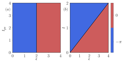
Figure 5: The phase diagram obtained via computing the Berry phase for the parameters (a) $\epsilon$ and $t_{ps}$ with $t=1$, and (b) $\epsilon$ and $t$, with $t_{ps}=1$. The phase diagrams show that the topological phase transition depends only on $\epsilon$ and $t$ regardless of the value of $t_{ps}$, and it occurs at $\epsilon=2t$. In the region, where $\epsilon<2t$, the Berry phase acquires a value $-\pi$ and $0$ for $\epsilon>2t$.

To obtain a phase diagram for the Berry phase using Eq.(21), we have considered the parameter space spanned by the onsite potential $\epsilon$ and the hopping strength $t_{ps}$, keeping $t$ fixed at $1$. As can be seen in Fig.5(a), there is a sharp transition in the value of the Berry phase depending on the values of $\epsilon$ and $t$, however, is independent of $t_{ps}$. Similarly, Fig.5(b) shows that the transition occurs along a straight line whose equation is $\epsilon=2t$. Above the line ($\epsilon<2t$), the Berry phase acquires a value $-\pi$ and below ($\epsilon>2t$) it vanishes. These are reminiscent of the appearance and disappearance of two (localized) zero energy edge states (shown in Figs.2(a) and 2(b)) and can be identified as the topological and the trivial phases respectively.

This phenomenon can also be explained from Fig.3. The ellipse (locus of the $\pmb{d^{\prime}_{1}}$-vector) contains the origin $(0,0)$ (topological case) for the case $\epsilon<2t$ and excludes when $\epsilon>2t$ (trivial case), which are suggestive of the phenomena of appearance and disappearance (Fig.2(b)) of zero energy eigenstates, respectively. The Hamiltonian $H_{1}$ becomes non-diagonalizable when the origin lies on the ellipse, that is, for $\epsilon=2t$, where the topological phase transition occurs.

III.2 Non-$\mathcal{PT}$ symmetric NH model

We now analyze the topological and localization properties of the NH model that includes staggered imaginary potential given by the Eqs.(8) and (9) in real and $k$-spaces, respectively. The potential $\pm i\epsilon$ on the $s$ and $p_{x}$ orbitals in the Hamiltonian $H_{2}$ physically imply ‘gain’ and ‘loss’ of energy that the system undergoes due to non-Hermiticity, and thus the eigenspectra become complex.

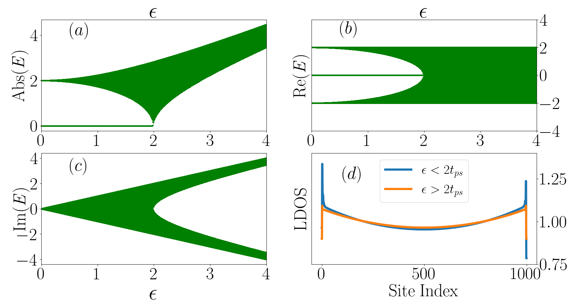
Figure 6: The (a) absolute values, (b) real part, and (c) imaginary part of the eigenvalues of $H_{2}$ (Eq.(8)) are plotted as a function of $\epsilon$. (c) shows the absence of purely real eigenvalues and hence is suggestive of a non-$\mathcal{PT}$ symmetric case. (a) and (b) show the appearance(disappearance) of absolute zero energy, that is, both the real and imaginary parts of the eigenvalues being zero and the edge states appear(disappear) for $\epsilon<2t_{ps}$($\epsilon>2t_{ps}$). (c) LDOS is calculated for both the topological and the trivial phases. The plot confirms the absence of NHSE.

The absolute value of the eigenspectra ($|E|$) is plotted as a function of $\epsilon$ with $t$ and $t_{ps}$ being kept fixed, ($t=t_{ps}=1$) in Fig.6(a), which shows that there are doubly degenerate zero energy edge modes that exist till $\epsilon=2$, and disappear beyond that. Fig.6(b), representing how the real part (Re($E$)) of the eigenvalues, $E$, varies with $\epsilon$, suggests that $E$ comes in pairs ($\pm E$) with their eigenvectors related by a unitary matrix, which is a manifestation of PHS. The real and imaginary parts, namely, Re($E$) and Im($E$) depend on the values of $t$, (shown by the constant width in Fig.6(b)) and $\epsilon$ (scales linearly as shown in Fig.6(c)), respectively. In Fig.6(d), we have shown the local density of states (LDOS), which can be obtained from the expression,

$$\mathrm{LDOS}^{(n)}=\sum_{i}|\psi_{n}^{i}|^{2}$$

at the $n^{\mathrm{th}}$ lattice site. The higher values of LDOS at the edges of the system for the case $\epsilon<2t_{ps}$ supports the existence of the two edge modes, which contrasts the case corresponding to $\epsilon>2t_{ps}$. It is clear from Fig.6(d) that the NHSE is absent in this system as there is no build-up of LDOS at one of the edges.

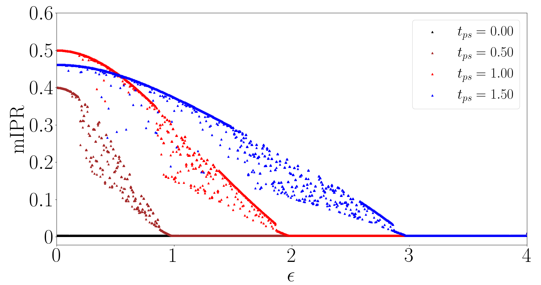
Figure 7: The maximum value of IPR, mIPR (defined in the text), versus $\epsilon$ is plotted here for different values of $t_{ps}$ keeping $t=1$. The plot suggests that the localization phase transitions now depend on $t_{ps}$. The scenario is unlike the Hermitian model, where it depends on $t$.

For a generic NH Hamiltonian (say $H_{NH}$), the right eigenvector, that is, the eigenvectors of $H_{NH}$ and left eigenvector (the eigenvectors of $H_{NH}^{\dagger}$) corresponding to a particular eigenvalue differ from each other. The orthonormality condition in this case is given by,

$$\left<\lambda_{m}|\psi_{n}\right>=\delta_{mn},$$

where $\ket{\lambda_{m}}$ and $\ket{\psi_{n}}$ are the left and the right eigenvectors corresponding to $m^{th}$ and $n^{th}$ eigenvalues of $H_{NH}^{\dagger}$ and $H_{NH}$ respectively [48, 49]. The IPR is given by the same formula as in Eq.(12), except for the fact that the right and the left eigenvectors will have to be used for this case. The mIPR, defined in the previous section, is computed as a function of $\epsilon$ for four different values of $t_{ps}$, namely, $t_{ps}=0,0.5,1,1.5$ and is shown in Fig.7. It is clear that the localization property of the model depends on $t_{ps}$. The mIPR is non-zero (edge states) for values of $\epsilon$ lower than $2t_{ps}$, and beyond that, it is zero, implying that all the states are localized to $\epsilon=2t_{ps}$, and are extended beyond that. The special case $t_{ps}=0$ denotes that for no inter-orbital hopping between different unit cells ($s-p_{x}$), the system behaves like a conductor owing to finite $t$ being present.

Next, we analyze the scenario with PBC. We perform the same unitary transformation as done in the previous section, given in Eq.(15), on the Bloch Hamiltonian, $h_{2}(k)$ in Eq(9) which yields,

$$h_{2}^{\prime}(k)=\begin{pmatrix}0&-i\epsilon+2t\cos k\\ &+2it_{ps}\sin k\\ -i\epsilon+2t\cos k\\ -2it_{ps}\sin k&0\end{pmatrix},$$ (22)

which can be written in a Dirac form as, $h^{\prime}_{2}(k)=\pmb{d^{\prime}_{2}}\cdot\pmb{\sigma}$ with $\pmb{d^{\prime}_{2}}\equiv(-i\epsilon+2t\cos k,-2t_{ps}\sin k,0)$. Evidently, $\pmb{d^{\prime}_{2}}$ has all the symmetries, that is, both PHS and $\textrm{TRS}^{\dagger}$, which eventually says that $\pmb{d_{2}}$ and $\pmb{d^{\prime}_{2}}$ have the same eigenspectra, and are given by,

$$E_{2\pm}(k)=\pm\sqrt{(-i\epsilon+2t\cos k)^{2}+4t_{ps}^{2}\sin^{2}k}.$$ (23)

The left ($\ket{\lambda^{\prime}_{2\pm}(k)}$) and the right ($\ket{\psi^{\prime}_{2\pm}(k)}$) eigenfunctions of $h^{\prime}_{2}(k)$ are given by,

$$\ket{\lambda^{\prime}_{2\pm}(k)} =\frac{1}{\sqrt{2}}e^{\pm i\eta^{*}}\begin{pmatrix}\pm e^{-i\phi_{2k}^{*}}\\ 1\end{pmatrix};$$

$$\ket{\psi^{\prime}_{2\pm}(k)} =\frac{1}{\sqrt{2}}e^{\pm i\eta}\begin{pmatrix}\pm e^{-i\phi_{2k}}\\ 1\end{pmatrix}.$$ (24)

Here $\eta$ is a constant (and independent of $k$ and $\phi_{2k}$), and $\phi_{2k}$ is given by,

$$\phi_{2k}=\tan^{-1}\left(\frac{2t_{ps}\sin k}{i\epsilon-2t\cos k}\right).$$

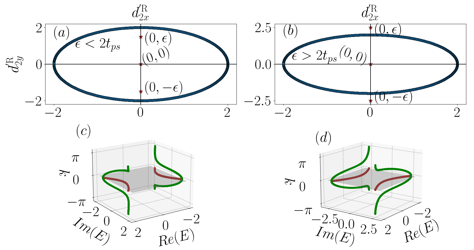
Figure 8: Real part of $\pmb{d^{\prime}_{2}}$-vector is drawn in a plane spanned by $d_{2x}^{{}^{\prime}\mathrm{R}}-d_{2y}^{{}^{\prime}\mathrm{R}}$ for the parameters $t=1$, $t_{ps}=1$, and (a) $\epsilon=1.5$, where the ellipse encloses the EPs (topological case), and (b) $\epsilon=2.5$, where it excludes the EPs (trivial case). (c) and (d) represent 3D figures of the band structures ($E(k)$ vs $k$) with the real and the imaginary parts of the energy being plotted along the $x$ and $y$ axis, respectively. At the same time, the momentum $k$ is along the $z$ direction. The points in green and brown denote the actual data points and their 2D projections, respectively.

Due to the non-Hermiticity of $h^{\prime}_{2}(k)$, $\pmb{d^{\prime}_{2}}$ is also complex unlike $\pmb{d^{\prime}_{1}}$. With the help of a little algebra, we can show that the locations of the two EPs in a space spanned by $d_{2x}^{{}^{\prime}\mathrm{R}}-d_{2y}^{{}^{\prime}\mathrm{R}}$ are at ($d_{2y}^{{}^{\prime}\mathrm{I}},-d_{2x}^{{}^{\prime}\mathrm{I}}$) and ($-d_{2y}^{{}^{\prime}\mathrm{I}},d_{2x}^{{}^{\prime}\mathrm{I}}$) [86] which are ($0,\epsilon$) and ($0,-\epsilon$) respectively, where $d_{2x}^{{}^{\prime}\mathrm{R}}$($d_{2y}^{{}^{\prime}\mathrm{R}}$) and $d_{2x}^{{}^{\prime}\mathrm{I}}$($d_{2y}^{{}^{\prime}\mathrm{I}}$) represent the real and the imaginary parts of $d^{\prime}_{2x}$($d^{\prime}_{2y}$) respectively. At these EPs, for $k=\frac{\pi}{2}$, $E_{2}(k)$ vanish and $\left<\lambda^{\prime}_{2\pm}(k)|\psi^{\prime}_{2\pm}(k)\right>$ becomes ill-defined. The locus of the real part of $\pmb{d^{\prime}_{2}}$ constitutes an ellipse with the center at ($0,0$) in the $d_{2x}^{{}^{\prime}\mathrm{R}}-d_{2y}^{{}^{\prime}\mathrm{R}}$ plane as shown in Figs.8(a) and 8(b) corresponding to two representative values of $\epsilon$, namely, $\epsilon=1.5$ and $\epsilon=2.5$ respectively. The region, where the EPs are inside(outside) the ellipse in Fig.8(a)(Fig.8(b)), which denotes $\epsilon<2t_{ps}$($\epsilon>2t_{ps}$), and is referred to the topological(trivial) phase with two(no) zero energy edge modes.

Further Figs.8(c) and 8(d) are the band structures for the same parameters as used in Figs.8(a) and 8(b), respectively. The plot shown in green color denotes $E_{2}(k)$ as a function of $k$, and the one in brown color represents the 2D projection of the same on the Re($E$)-Im($E$) plane. Fig.8(c), which corresponds to the topological phase, shows that there is a real line gap in the band structure as,

$$\mathrm{Re}(E_{2}(k))\neq 0\;\forall\;k.$$

The base axis is the imaginary axis, with the projected $E_{2}(k)$ lying on either side of the base axis. At $\epsilon=2t_{ps}$, the two bands are intertwined at the points $-\frac{\pi}{2}$, $0$ and $\frac{\pi}{2}$ in the BZ. Thus the Hamiltonian becomes gapless at these points, where the topological to the trivial phase transition occurs. In contrast, in Fig.8(d), for $\epsilon>2t_{ps}$, the line gap becomes imaginary, with the base axis now being replaced by the real axis, and the system is in a trivial phase.

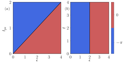
Figure 9: Phase diagram based on the value of CBP for the parameters (a) $\epsilon$ and $t_{ps}$ keeping $t=1$ and (b) $\epsilon$ and $t$ keeping $t_{ps}$ fixed at $1$. The phase diagrams suggest that the values of CBP depend only on $\epsilon$ and $t_{ps}$ and are independent of the values of $t$. The CBP takes the values $-\pi$ and $0$ for the regions $\epsilon<2t_{ps}$ and $\epsilon>2t_{ps}$, respectively.

The origin of the complex Berry phase (CBP) [79], which denotes the topological invariant for the present case, remains equivalent to that for the Hermitian case with the only difference that now the left and right eigenvectors have to be employed. Thus, the definition of the CBP becomes,

$$\gamma_{\pm}=i\oint_{BZ}\bra{\lambda^{\prime}_{2\pm}(k)}\nabla_{k}\ket{\psi^{\prime}_{2\pm}(k)}\;dk.$$ (25)

Substituting the expressions of $\ket{\lambda^{\prime}_{2\pm}(k)}$ and $\ket{\psi^{\prime}_{2\pm}(k)}$ in Eq.(24) in Eq.(25), we get the expression for CBP,

$$\gamma_{\pm} =\frac{1}{2}\oint_{BZ}\frac{\partial\phi_{2k}}{\partial k}\;dk$$

$$=\frac{1}{2}\oint_{BZ}\frac{2t_{ps}(i\epsilon\cos k-2t)}{(-i\epsilon+2t\cos k)^{2}+4t_{ps}^{2}\sin^{2}k}\;dk$$ (26)

From the above equation, we get the phase diagram shown in Fig.9, where CBP is computed for a range of $\epsilon$, namely, [$0:4$]. Fig.9(a) suggests that a phase transition occurs across the straight line denoted by $\epsilon=2t_{ps}$. Fig.9(b) depicts the values of CBP in the $t$-$\epsilon$ plane ($t_{ps}=1$). The plot suggests that CBP is independent of $t$, however, changes value from $-\pi$ to $0$ at $\epsilon=2t_{ps}$, denoting that these are the topological and the trivial phases, respectively. These phenomena are almost the same as the previous (Hermitian) case (see Fig.5), except for the fact that the roles of $t$ and $t_{ps}$ are interchanged with regard to the topological phase transitions Also, the bi-orthogonal BBC [48] is preserved here as NHSE is not realized.

III.3 $\mathcal{PT}$ symmetric NH model

The second NH variant is obtained by putting a non-reciprocity term ($\delta$) only in the hopping amplitudes between the different orbitals ($t_{ps}$) of the neighboring unit cells. We shall explore the evolution of properties by varying the parameters, $\epsilon$ (onsite potential) and $\delta$ (non-reciprocity). The eigenspectra in real space for the Hamiltonian, given by Eq.(10), is plotted in Fig.10 for $\epsilon<2t$.

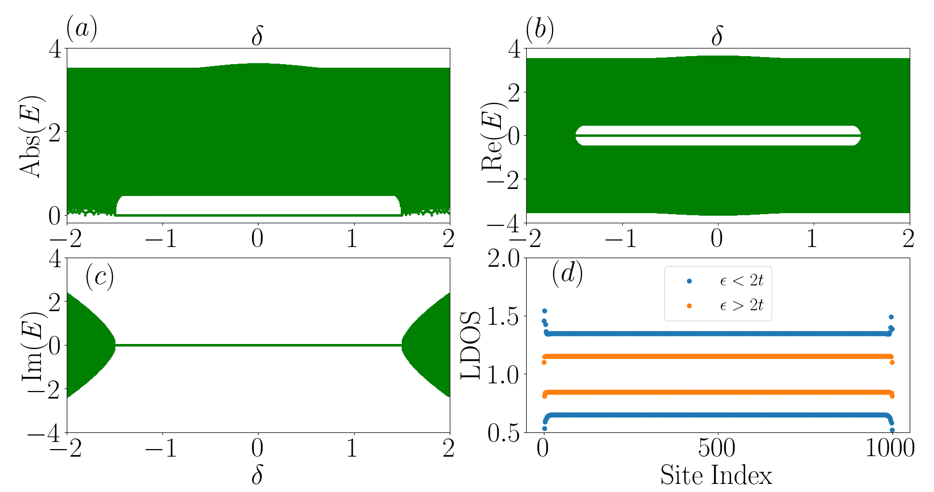
Figure 10: The (a) absolute values, (b) real part, (c) imaginary part of eigenspectra are plotted aa s function of the non-reciprocity parameter, $\delta$, with $\epsilon=1.5t$, $t=t_{ps}=1$. (d) The LDOS is calculated for $\epsilon=1.5$ ($<2t$) and $\epsilon=3$ ($>2t$). The LDOS confirms of an absence of NHSE.

Fig.10(a) shows the dependence of $|E|$ on $\delta$. Figs.10(b) and 10(c) show the real part (Re($E$)) and the imaginary part (Im($E$)) of the eigenvalues. The plot indicates that the energies appear both as ($E,E^{*}$) and ($E,-E$) pairs due to the presence of TRS and PHS, respectively. Im($E$) is zero as long as the condition $|\delta|\leq t_{ps}$ is satisfied, suggesting that this is the $\mathcal{PT}$-unbroken phase [1]. Beyond which, that is, for $|\delta|>t_{ps}$, Im($E$) becomes non-zero, indicating that the system has entered into a $\mathcal{PT}$-broken phase. Fig.10(d) represents the LDOS plots via two pairs of flat ‘lines’ corresponding to $\epsilon<2t$ (lines in blue) and $\epsilon>2t$ (lines in orange). These lines denote discrete values of LDOS at the lattice sites and oscillate from one site to the next. Further, for $\epsilon<2t$, the blue lines demonstrate the existence of edge modes via higher values at the extremities, while the orange ones do not have such signatures. Moreover, there is no sign of NHSE seen here.

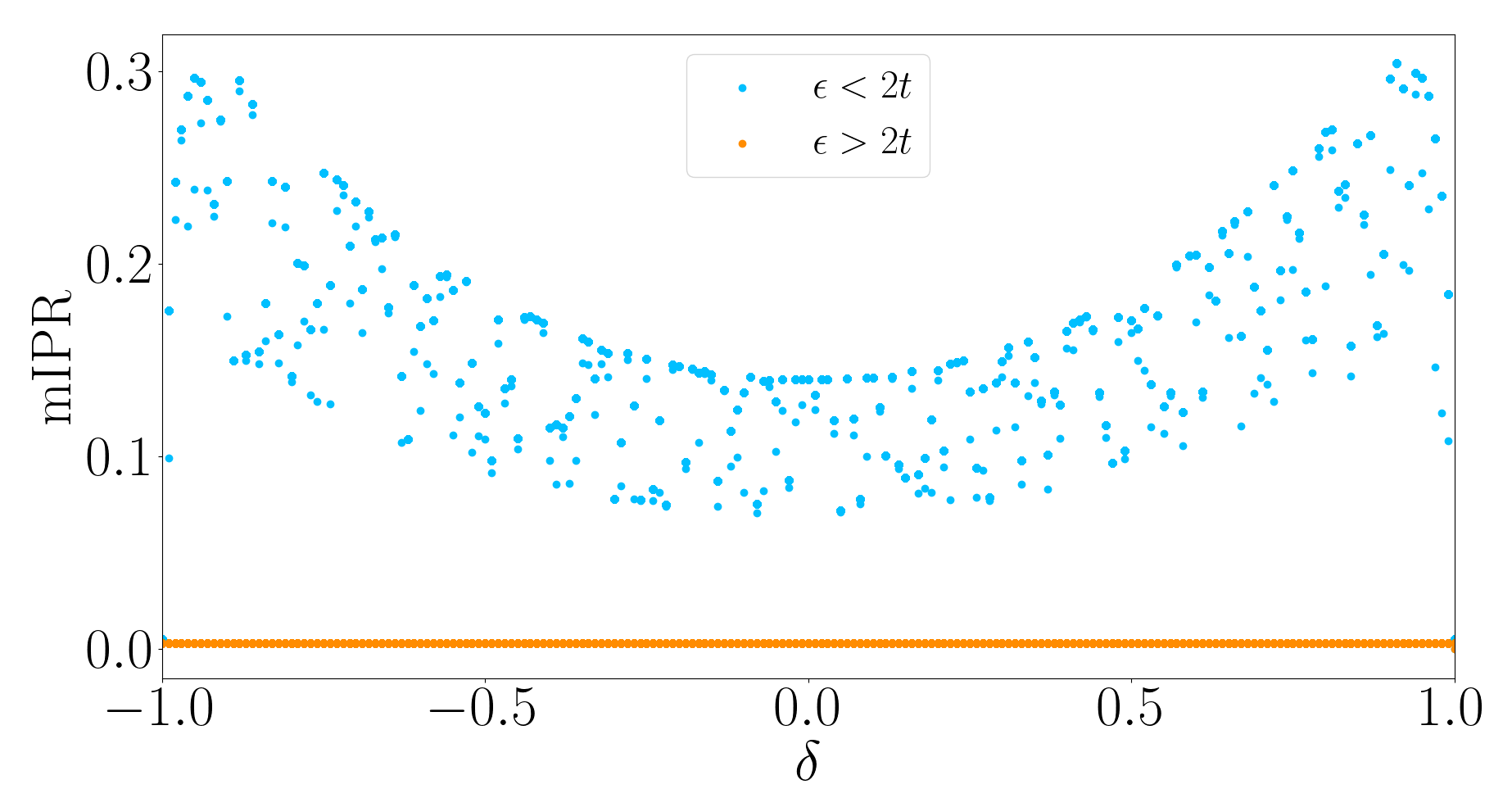
Figure 11: The mIPR is varied with $\delta$ for $t=t_{ps}=1$ corresponding to the cases $\epsilon=1.5$ ($<2t$) and $\epsilon=3$ ($>2t$), respectively.

The localization of these edge states, measured by mIPR, is shown in Fig.11 as a function of the non-reciprocity parameter, $\delta$, in the range [$-1:1$]. The mIPR is non-zero for $\epsilon<2t$ and supports the existence of the $|E|=0$ states that are localized at the edges, suggesting that this is a topological phase. As $|\delta|$ increases, the energy required for hopping (which is $t_{ps}+|\delta|$) increases as well, which results in a localization scenario at the edges of the chain, and hence is suggestive of higher mIPR values. These edge modes vanish as soon as $\epsilon$ becomes larger than $2t$ when all the eigenstates become extended and mIPR vanishes. Further, the system enters into a trivial phase, and the phase transition occurs at $\epsilon=2t$.

Now, we shall analyze the infinite system in $k$-space through the Bloch Hamiltonian given in Eq.(11) in order to establish a correspondence with the finite system in real space. This will aid us in showing that bi-orthogonal BBC is preserved here, similar to the non-$\mathcal{PT}$ symmetric case. We shall proceed in the same manner as in the previous sections; that is, the basis of the Bloch Hamiltonian will be rotated via a unitary operator, $U$, given in Eq.(15). After rotation, the Bloch Hamiltonian, let us call it $h^{\prime}_{3}(k)$, is given by,

$$h^{\prime}_{3}(k)=\begin{pmatrix}2i\delta\sin k&-\epsilon+2t\cos k\\ &+2it_{ps}\sin k\\ -\epsilon+2t\cos k\\ -2it_{ps}\sin k&-2i\delta\sin k\end{pmatrix},$$ (27)

with $\pmb{d^{\prime}_{3}}\equiv(-\epsilon+2t\cos k,-2t_{ps}\sin k,2i\delta\sin k)$, suggesting that all, but the $z$ component of $\pmb{d^{\prime}_{3}}$ is real, that is,

$$d_{3x}^{{}^{\prime}\mathrm{R}} =-\epsilon+2t\cos k,\;d_{3y}^{{}^{\prime}\mathrm{R}}=-2t_{ps}\sin k,\;d_{3z}^{{}^{\prime}\mathrm{R}}=0;$$

$$d_{3x}^{{}^{\prime}\mathrm{I}} =0,\;d_{3y}^{{}^{\prime}\mathrm{I}}=0,\;d_{3z}^{{}^{\prime}\mathrm{I}}=2i\delta\sin k,$$

where the notations bear a similar meaning as given in the previous section. It is clear that $h^{\prime}_{3}(k)$ commutes with the $\mathcal{PT}$ operator given by $\sigma_{x}\mathcal{K}$ and hence preserves $\mathcal{PT}$ symmetry. The expression for the band structure, which is the same for both $h_{3}(k)$ and $h^{\prime}_{3}(k)$, is given by,

$$E_{3\pm}(k) =\pm\sqrt{(d_{3x}^{{}^{\prime}\mathrm{R}}+id_{3x}^{{}^{\prime}\mathrm{I}})^{2}+(d_{3y}^{{}^{\prime}\mathrm{R}}+id_{3y}^{{}^{\prime}\mathrm{I}})^{2}+(d_{3z}^{{}^{\prime}\mathrm{R}}+id_{3z}^{{}^{\prime}\mathrm{I}})^{2}}$$

$$=\pm\sqrt{(-\epsilon+2t\cos k)^{2}+4(t_{ps}^{2}-\delta^{2})\sin^{2}k}.$$ (28)

Moreover, the left and the right eigenvectors of $h^{\prime}_{3}(k)$ are given by,

$$\ket{\lambda^{\prime}_{3\pm}(k)} =\pm\frac{1}{\sqrt{2}}\beta_{1}e^{\pm i\alpha^{*}}\begin{pmatrix}\frac{\sin\theta^{*}_{k}e^{-i\phi_{3k}}}{\pm 1+\cos\theta^{*}_{k}}\\ 1\end{pmatrix};$$

$$\ket{\psi^{\prime}_{3\pm}(k)} =\pm\frac{1}{\sqrt{2}}\beta_{2}e^{\pm i\alpha}\begin{pmatrix}\frac{\sin\theta_{k}e^{-i\phi_{3k}}}{\pm 1-\cos\theta_{k}}\\ 1\end{pmatrix},$$ (29)

where $\alpha$ is independent of $k$ and $\phi_{3k}$ and $\theta_{k}$ are given by,

$$\phi_{3k} =\tan^{-1}\left[\frac{-2t_{ps}\sin k}{-\epsilon+2t\cos k}\right];$$

$$\theta_{k} =\tan^{-1}\left[\frac{\sqrt{(-\epsilon+2t\cos k)^{2}+4t_{ps}^{2}\sin^{2}k}}{2i\delta\sin k}\right].$$

$\beta_{1}$ and $\beta_{2}$ satisfy the relation,

$$\beta^{*}_{1}\beta_{2}=\frac{1}{2}(1-\cos\theta_{k})$$

and are periodic functions of $k$.

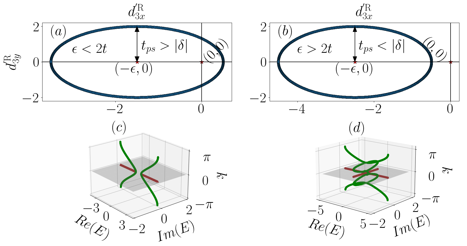
Figure 12: The locus of the $\pmb{d^{\prime}_{3}}$-vector is drawn in a plane spanned by $d_{3x}^{{}^{\prime}\mathrm{R}}-d_{3y}^{{}^{\prime}\mathrm{R}}$ for the parameters $t=1$, $t_{ps}=1$ and (a) $\epsilon=1.5$, where the ellipse contains the origin ($0,0$) (topological case) and (b) $\epsilon=2.5$, where it excludes the origin (trivial case). (c) and (d) represent 3D figures of the band structures ($E(k)$ vs $k$) with the real and the imaginary parts of the energy and the momentum ($k$) being plotted along the $x$, $y$, and $z$ directions, respectively. The parameters are the same as those of (a) and (b). The points in green and brown are the actual data points and their 2D projections, respectively.

The energy $E_{3}(k)$ in Eq.(28) becomes zero when $d_{3x}^{{}^{\prime}\mathrm{R}}=0$ and $d_{3y}^{{}^{\prime}\mathrm{R}}=|d_{3z}^{{}^{\prime}\mathrm{I}}|$. These two are the conditions for an EP. Putting these conditions in Eq.(29), we see that,

$$\left<\lambda^{\prime}_{3\pm}(k)|\psi^{\prime}_{3\pm}(k)\right>=0.$$

This tells us that the bi-orthogonality condition is breaking down at the EP.

Similar picture emerges for Figs.12(a) and 12(b), where the trajectory of $\pmb{d^{\prime}_{3}}$, which is an ellipse, is represented in a plane spanned by $d_{3x}^{{}^{\prime}\mathrm{R}}-d_{3y}^{{}^{\prime}\mathrm{R}}$ for two values of $\epsilon$, namely, $\epsilon=1.5$ and $\epsilon=2.5$, respectively. In Fig.12(a), the origin ($0,0$) is inside the ellipse. The length of the semi-minor axis, which is $t_{ps}$, is greater than $|\delta|$, suggesting that it denotes a topological phase. On the other hand, Fig.12(b) describes the trivial case as the ellipse excludes the origin, that is, $\epsilon>2t$. Thus, we can conclude that the EP for the present case is the origin but with a condition, namely, $t_{ps}=|\delta|$. Fig.12(c) shows the case where $\mathcal{PT}$ symmetry is still unbroken since the conditions $\epsilon<2t$ and $|\delta|<t_{ps}$ are satisfied, resulting in the eigenspectra to be purely real (the imaginary part being zero shown by the brown line). Unlike the non-$\mathcal{PT}$ symmetric case, the energy gap, in this case, represents a point gap. It closes when $|\delta|=t_{ps}$ is satisfied with the condition $\epsilon<2t$. Note that, for $\epsilon<2t$, the sufficient condition for the eigenspectra to be purely real is $|\delta|<t_{ps}$, but for $\epsilon>2t$, the necessary condition for at least one (pair of) eigenvalue(s) to be complex is $|\delta|>\sqrt{t_{ps}^{2}+\frac{\epsilon^{2}}{4}}$. This phenomenon corresponds to the $\mathcal{PT}$-broken phase and is shown in Fig.12(d), where some of the eigenvalues become purely imaginary, and the point gap reopens. Putting $\ket{\lambda^{\prime}_{3\pm}(k)}$ and $\ket{\psi^{\prime}_{3\pm}(k)}$ from Eq.(29) into Eq.(25), we get an expression for the CBP as,

$$\gamma_{\pm} =\frac{1}{2}\oint_{BZ}\frac{\partial\phi_{3k}}{\partial k}(1+\cos\theta_{k})\;dk$$

$$=\frac{1}{2} \oint_{BZ}\frac{2t_{ps}(\epsilon\cos k-2t)}{(-\epsilon+2t\cos k)^{2}+4t_{ps}^{2}\sin^{2}k}\left(1+\frac{2i\delta\sin k}{E_{3+}(k)}\right)dk$$ (30)

The phase diagram of CBP obtained from the Eq.(30) is exactly similar to that of the Fig.5 (and hence not shown again), hinting that the topological phase transition occurs at $\epsilon=2t$ for $|\delta|<t_{ps}$.

IV Conclusion

We have taken a two-orbital NH version of a 1D tight-binding model in our work. A study of the Hermitian model is included for the purpose of comparison whose trivial and the non-trivial phases depend on the competition between the onsite potential, $\epsilon$ and the hopping amplitude, $t$. Further, the description of the NH extension of the model has been fragmented into a non-$\mathcal{PT}$ symmetric (one with onsite imaginary potential), and a $\mathcal{PT}$ symmetric (one with non-reciprocal hopping amplitudes) version. Both obey a bi-orthogonal BBC, which in turn implies the absence of NHSE. These results are supported by computing the LDOS. The topological invariant, namely, the CBP for both the NH systems yields values $0$ or $-\pi$, corresponding to them being in trivial or topological phases, respectively. Moreover, the emergence of the zero energy edge modes is realized through the confinement of the EPs and demonstrated via corresponding $\pmb{d}$-vectors in $k$-space. The significant differences between the models are: (i) the key parameters that decide the phase transition for a trivial to a topological phase (or a localized to delocalized phase) are the inter-orbital ($t_{ps}$) and intra-orbital ($t$) hopping amplitudes, and (ii) the complex energy gaps, namely, the line gap and the point gap, corresponding to the non-$\mathcal{PT}$ symmetric and $\mathcal{PT}$ symmetric cases, respectively. However, the $\mathcal{PT}$ symmetry gets broken spontaneously even in the $\mathcal{PT}$ symmetric system depending on the values of the parameters. Thus, two different regimes emerge, where the $\mathcal{PT}$ unbroken regime hosts purely real eigenvalues, while complex eigenvalues appear in the $\mathcal{PT}$ broken phase.

References

- Bender and Boettcher [1998] C. M. Bender and S. Boettcher, Phys. Rev. Lett. 80, 5243 (1998).
- Bender et al. [1999] C. M. Bender, S. Boettcher, and P. N. Meisinger, Journal of Mathematical Physics 40, 2201 (1999).
- Bender et al. [2002] C. M. Bender, D. C. Brody, and H. F. Jones, Phys. Rev. Lett. 89, 270401 (2002).
- Mostafazadeh and Batal [2004] A. Mostafazadeh and A. Batal, Journal of Physics A: Mathematical and General 37, 11645 (2004).
- Moiseyev [2011] N. Moiseyev, Non-Hermitian Quantum Mechanics (Cambridge University Press, 2011).
- El-Ganainy et al. [2018] R. El-Ganainy et al., Nat. Phys. 14 (2018), 10.1038/nphys4323.
- Rüter et al. [2010] C. E. Rüter et al., Nat. Phys. 6 (2010), 10.1038/nphys1515.
- Eichelkraut et al. [2013] T. Eichelkraut et al., Nat. Commun. 4 (2013), 10.1038/ncomms3533.
- Peng et al. [2014] B. Peng et al., Nat. Phys. 10 (2014), 10.1038/nphys2927.
- Feng et al. [2014] L. Feng, Z. J. Wong, R.-M. Ma, Y. Wang, and X. Zhang, Science 346 (2014), 10.1126/science.1258479.
- Xiao et al. [2017] L. Xiao et al., Nat. Phys. 13 (2017), 10.1038/nphys4204.
- Bahari et al. [2017] B. Bahari, A. Ndao, F. Vallini, A. E. Amili, Y. Fainman, and B. Kanté, Science 358, 636 (2017).
- Weimann et al. [2017] S. Weimann, M. Kremer, and Y. Plotnik, Nat. Mater. 16 (2017), 10.1038/nmat4811.
- St-Jean et al. [2017] P. St-Jean, V. Goblot, and E. Galopin, Nat. Photonics 11 (2017), 0.1038/s41566-017-0006-2.
- Xiao et al. [2019] L. Xiao et al., Phys. Rev. Lett. 123, 230401 (2019).
- Xiao et al. [2020] L. Xiao, T. Deng, and K. Wang, Nat. Phys. 16 (2020), 10.1038/s41567-020-0836-6.
- Rosenthal et al. [2018] E. I. Rosenthal et al., Phys. Rev. B 97, 220301 (2018).
- Sakhdari et al. [2019] M. Sakhdari et al., Phys. Rev. Lett. 123, 193901 (2019).
- Li et al. [2020] L. Li, C. H. Lee, S. Mu, and J. Gong, Nat. Commun. 11 (2020), 10.1038/s41467-020-18917-4.
- Helbig et al. [2020] T. Helbig et al., Nat. Phys. 16 (2020), 10.1038/s41567-020-0922-9.
- Stegmaier et al. [2021] A. Stegmaier et al., Phys. Rev. Lett. 126, 215302 (2021).
- Fleury et al. [2015] R. Fleury, D. Sounas, and A. Alù, Nat. Commun. 6 (2015), 10.1038/ncomms6905.
- Rosendo López et al. [2019] M. Rosendo López, Z. Zhang, D. Torrent, and J. Christensen, Nat. Commun. 2 (2019), 10.1038/s42005-019-0233-6.
- Zhang et al. [2019] Z. Zhang, M. Rosendo Lopez, Y. Cheng, X. Liu, and J. Christensen, Phys. Rev. Lett. 122, 195501 (2019).
- Gu et al. [2021] Z. Gu, H. Gao, P.-C. Cao, T. Liu, X.-F. Zhu, and J. Zhu, Phys. Rev. Appl. 16, 057001 (2021).
- Zhang et al. [2021] L. Zhang et al., Commun. Phys. 12 (2021), 10.1038/s41467-021-26619-8.
- Gao et al. [2021] H. Gao, H. Xue, Z. Gu, T. Liu, J. Zhu, and B. Zhang, Nat. Commun. 12 (2021), 10.1038/s41467-021-22223-y.
- Thouless et al. [1982] D. J. Thouless, M. Kohmoto, M. P. Nightingale, and M. den Nijs, Phys. Rev. Lett. 49, 405 (1982).
- Hasan and Kane [2010] M. Z. Hasan and C. L. Kane, Rev. Mod. Phys. 82, 3045 (2010).
- Qi and Zhang [2011] X.-L. Qi and S.-C. Zhang, Rev. Mod. Phys. 83, 1057 (2011).
- Chiu et al. [2016] C.-K. Chiu, J. C. Y. Teo, A. P. Schnyder, and S. Ryu, Rev. Mod. Phys. 88, 035005 (2016).
- Kane and Mele [2005a] C. L. Kane and E. J. Mele, Phys. Rev. Lett. 95, 226801 (2005a).
- Fu et al. [2007] L. Fu, C. L. Kane, and E. J. Mele, Phys. Rev. Lett. 98, 106803 (2007).
- Su et al. [1979] W. P. Su, J. R. Schrieffer, and A. J. Heeger, Phys. Rev. Lett. 42, 1698 (1979).
- Su et al. [1980] W. P. Su, J. R. Schrieffer, and A. J. Heeger, Phys. Rev. B 22, 2099 (1980).
- Haldane [1988] F. D. M. Haldane, Phys. Rev. Lett. 61, 2015 (1988).
- Kane and Mele [2005b] C. L. Kane and E. J. Mele, Phys. Rev. Lett. 95, 146802 (2005b).
- Altland and Zirnbauer [1997] A. Altland and M. R. Zirnbauer, Phys. Rev. B 55, 1142 (1997).
- Teo and Kane [2010] J. C. Y. Teo and C. L. Kane, Phys. Rev. B 82, 115120 (2010).
- Berry [1984] M. V. Berry, Proceedings of the Royal Society A 392 (1984), 10.1098/rspa.1984.0023.
- Berry [1985] M. V. Berry, Journal of Physics A: Mathematical and General 18, 15 (1985).
- Schomerus [2013] H. Schomerus, Opt. Lett. 38, 1912 (2013).
- Hatano and Nelson [1996] N. Hatano and D. R. Nelson, Phys. Rev. Lett. 77, 570 (1996).
- Rudner and Levitov [2009] M. S. Rudner and L. S. Levitov, Phys. Rev. Lett. 102, 065703 (2009).
- Hu and Hughes [2011] Y. C. Hu and T. L. Hughes, Phys. Rev. B 84, 153101 (2011).
- Esaki et al. [2011] K. Esaki, M. Sato, K. Hasebe, and M. Kohmoto, Phys. Rev. B 84, 205128 (2011).
- Lee [2016] T. E. Lee, Phys. Rev. Lett. 116, 133903 (2016).
- Kunst et al. [2018] F. K. Kunst, E. Edvardsson, J. C. Budich, and E. J. Bergholtz, Phys. Rev. Lett. 121, 026808 (2018).
- Lieu [2018] S. Lieu, Phys. Rev. B 97, 045106 (2018).
- Yao and Wang [2018] S. Yao and Z. Wang, Phys. Rev. Lett. 121, 086803 (2018).
- Edvardsson et al. [2019] E. Edvardsson, F. K. Kunst, and E. J. Bergholtz, Phys. Rev. B 99, 081302 (2019).
- Jin and Song [2019] L. Jin and Z. Song, Phys. Rev. B 99, 081103 (2019).
- Smilga [2009] A. V. Smilga, Journal of Physics A: Mathematical and Theoretical 42, 095301 (2009).
- Kato [2012] T. Kato, Perturbation Theory for Linear Operators (Springer Berlin, Heidelberg, 2012).
- Heiss [2012] W. D. Heiss, Journal of Physics A: Mathematical and Theoretical 45, 444016 (2012).
- Minganti et al. [2019] F. Minganti, A. Miranowicz, R. W. Chhajlany, and F. Nori, Phys. Rev. A 100, 062131 (2019).
- Chen et al. [2019] C. Chen, L. Jin, and R.-B. Liu, New Journal of Physics 21, 083002 (2019).
- Ozdemir et al. [2019] S. K. Ozdemir, S. Rotter, F. Nori, and L. Yang, Nat. Mater. 18 (2019), 10.1038/s41563-019-0304-9.
- Shnerb and Nelson [1998] N. M. Shnerb and D. R. Nelson, Phys. Rev. Lett. 80, 5172 (1998).
- Gong et al. [2018] Z. Gong, Y. Ashida, K. Kawabata, K. Takasan, S. Higashikawa, and M. Ueda, Phys. Rev. X 8, 031079 (2018).
- Yuce [2020] C. Yuce, Physics Letters A 384, 126094 (2020).
- Okuma et al. [2020] N. Okuma, K. Kawabata, K. Shiozaki, and M. Sato, Phys. Rev. Lett. 124, 086801 (2020).
- Song et al. [2020] Y. Song, W. Liu, L. Zheng, Y. Zhang, B. Wang, and P. Lu, Phys. Rev. Appl. 14, 064076 (2020).
- Longhi [2020] S. Longhi, Phys. Rev. B 102, 201103 (2020).
- Kawabata et al. [2020] K. Kawabata, M. Sato, and K. Shiozaki, Phys. Rev. B 102, 205118 (2020).
- Borgnia et al. [2020] D. S. Borgnia, A. J. Kruchkov, and R.-J. Slager, Phys. Rev. Lett. 124, 056802 (2020).
- Zhu et al. [2020] X. Zhu, H. Wang, S. K. Gupta, H. Zhang, B. Xie, M. Lu, and Y. Chen, Phys. Rev. Res. 2, 013280 (2020).
- Shen et al. [2018] H. Shen, B. Zhen, and L. Fu, Phys. Rev. Lett. 120, 146402 (2018).
- Yokomizo and Murakami [2019] K. Yokomizo and S. Murakami, Phys. Rev. Lett. 123, 066404 (2019).
- Ashida et al. [2020] Y. Ashida, Z. Gong, and M. Ueda, Advances in Physics 69, 249 (2020).
- Kawabata et al. [2019a] K. Kawabata, K. Shiozaki, M. Ueda, and M. Sato, Phys. Rev. X 9, 041015 (2019a).
- Ghatak and Das [2019] A. Ghatak and T. Das, Journal of Physics: Condensed Matter 31, 263001 (2019).
- Bergholtz et al. [2021] E. J. Bergholtz, J. C. Budich, and F. K. Kunst, Rev. Mod. Phys. 93, 015005 (2021).
- Bernevig et al. [2006] B. A. Bernevig, T. L. Hughes, and S.-C. Zhang, Science 314, 1757 (2006).
- Fu and Kane [2007] L. Fu and C. L. Kane, Phys. Rev. B 76, 045302 (2007).
- Kawabata et al. [2018] K. Kawabata, K. Shiozaki, and M. Ueda, Phys. Rev. B 98, 165148 (2018).
- Ozcakmakli Turker and Yuce [2019] Z. Ozcakmakli Turker and C. Yuce, Phys. Rev. A 99, 022127 (2019).
- Kawabata and Sato [2020] K. Kawabata and M. Sato, Phys. Rev. Res. 2, 033391 (2020).
- Garrison and Wright [1988] J. Garrison and E. Wright, Physics Letters A 128, 177 (1988).
- Dattoli et al. [1990] G. Dattoli, R. Mignani, and A. Torre, Journal of Physics A: Mathematical and General 23, 5795 (1990).
- Mostafazadeh [1999] A. Mostafazadeh, Physics Letters A 264, 11 (1999).
- Schnyder et al. [2008] A. P. Schnyder, S. Ryu, A. Furusaki, and A. W. W. Ludwig, Phys. Rev. B 78, 195125 (2008).
- Ryu et al. [2010] S. Ryu, A. P. Schnyder, A. Furusaki, and A. W. W. Ludwig, New Journal of Physics 12, 065010 (2010).
- Kawabata et al. [2019b] K. Kawabata, S. Higashikawa, Z. Gong, Y. Ashida, and M. Ueda, Nat. Commun. 10 (2019b), 10.1038/s41467-018-08254-y.
- Kramer and MacKinnon [1993] B. Kramer and A. MacKinnon, Reports on Progress in Physics 56, 1469 (1993).
- Yin et al. [2018] C. Yin, H. Jiang, L. Li, R. Lü, and S. Chen, Phys. Rev. A 97, 052115 (2018).