A Multi-Task Approach to Robust Deep Reinforcement Learning for Resource Allocation

Abstract

With increasing complexity of modern communication systems, Machine Learning (ML) algorithms have become a focal point of research. However, performance demands have tightened in parallel to complexity. For some of the key applications targeted by future wireless, such as the medical field, strict and reliable performance guarantees are essential, but vanilla ML methods have been shown to struggle with these types of requirements. Therefore, the question is raised whether these methods can be extended to better deal with the demands imposed by such applications. In this paper, we look at a combinatorial Resource Allocation (RA) challenge with rare, significant events which must be handled properly. We propose to treat this as a multi-task learning problem, select two methods from this domain, Elastic Weight Consolidation (EWC) and Gradient Episodic Memory (GEM), and integrate them into a vanilla actor-critic scheduler. We compare their performance in dealing with Black Swan Events with the state-of-the-art of augmenting the training data distribution and report that the multi-task approach proves highly effective.

I Introduction

As the journey towards the 6th generation 3GPP mobile communication standard continues, many of the most noteworthy targeted use cases are becoming highly specific, with requirements more extreme and heterogeneous [1, 2]. While the average user may be satisfied with the service provided by 5G NR, as it is currently being implemented by telecommunications service providers world wide, application fields such as medical communications have demands in, e.g., bit rate, latency, and reliability that are edge cases even in 5G NR [3, 4]. Among the many challenges faced in implementing efficient communication networking, the task of RA is among those that may limit performance the most. A capable resource scheduler must consider and balance available information, demands, and potential constraints in order to find an optimal allocation solution. For applications with heterogeneous service demands, the combinatorial problems found in resource allocation can quickly become burdensome to solve optimally in real time [5]. For this reason, RA has attracted significant interest in applying ML [6].

ML, and, in particular, Deep Learning (DL), have recently demonstrated strong performance in data driven function approximation in multiple domains, remarkably so in language and image processing, which are traditionally considered highly complex to solve well. Their strength lies in the ability to infer an approximately optimal solution from a given data set without the need to try to model the underlying processes. Instead, for example, the subdomain of Reinforcement Learning (RL) learns by “trial and error”, roughly trying to increase the likelihood of decisions that show to produce useful results while avoiding those that do not. First results in applying RL to the task of RA in wireless communication have shown promising results, e.g., [7, 8, 9]. For especially demanding applications, however, some issues remain with these approximated algorithms. While a visual glitch may be frustrating in image generation, a missed emergency transmission may prove fatal. Unfortunately, some of the more potent ML algorithms have been shown to struggle learning from data samples that are underrepresented in the overall data set [10].

A typical approach to helping this issue in communication systems is to artificially increase the relative amount of priority events in the learning data set, by, e.g., influencing data generation [9] or jointly training on two data sets [11] with tailored distributions. Experience from domains like autonomous driving shows that algorithms trained this way, i.e., trained on a data distribution that does not match reality, may struggle to reach expected performance when applied to the desired application [12]. Further, with more complex applications, finding and generating the correct augmented data set that induces the desired behavior in the learned algorithm becomes a taxing and non-intuitive task. Lastly, these methods have no protection against catastrophic forgetting [13], i.e., overwriting desired behavior if learning is continued on new data with a lack of priority events.

We present a procedure to harden RL schedulers in the presence of rare events by a multi-task learning approach. Considering the task of discrete resource scheduling on the MAC layer, the learned scheduler will have to solve three conflicting objectives: 1) Maximizing Sum-Rate, 2) minimizing time outs, and especially 3) minimizing time outs on rare events that demand very low latency. We show that, by default, the scheduler is not able to learn proper management of these rare priority events. Therefore, we make use of methods from multi-task learning, where a single learned algorithm must sequentially learn multiple different tasks with limited loss in performance on earlier tasks. We define our first task, that we wish to learn to satisfaction and then prevent unlearning, as the handling of priority messages with high reliability. Subsequently, we then integrate two methods from multi-task learning with a vanilla deep RL resource scheduler which we used in [14]. We show that the two methods,

1. EWC [13], presented in our work [15]. EWC imposes an elastic penalty onto the learning objective, incentivizing learning steps that cause the least change in expected behavior on scheduling priority events by way of Fisher information;

2. GEM [16] proposes to foster positive transfer learning between tasks by only allowing learning steps that do not cause negative impact on a representative set of priority event data samples,

are competitive in performance to the default approach of augmenting the learning data distribution while also compensating the issues mentioned earlier.

In the following, we will start by introducing the RA system model and optimization objective. We then recapitulate the design of a deep RL scheduler, and detail the workings of the two multi-task learning methods and their integration with the RL scheduler. We then evaluate and discuss their performance, advantages, and drawbacks.

Preliminaries & Notation: This paper assumes knowledge of stochastic gradient descent optimization and feed-forward Neural Networks. Vectors and matrices are denoted in boldface ($\mathbf{x}$), sets in blackboard-boldface ($\mathbb{N}$).

II System Model

In this section, we will first introduce the specifics of the discrete frequency allocation problem with significant rare events. We then formulate a heterogeneous utility function that is to be optimized.

II-A Discrete Resource Allocation

Several of the currently used medium access control protocols, chiefly among them the widely used Orthogonal Frequency Division Multiplex (OFDM), separate the available resource bandwidth into discrete blocks. Therefore, we consider a RA problem as depicted in Fig. 1, where in every discrete time step $t$ a scheduler at a base station is presented with a set of jobs $\mathbb{J}_{\text{req},t}$. Each job $j$ is destined for a specific user $n\in\mathbb{N}$ from a total of $N\in\mathbb{N}$ users and comes with a number of properties, to be specified subsequently. Based on the state of these properties, the scheduler must then distribute the total number of $U\in\mathbb{N}$ available discrete resource slots among the $N$ users in order to maximize a utility function, to be defined in subsection Section II-B. The decision takes the form of an allocation vector

$$\mathbf{A}_{t}=\left[a_{1},\,a_{2},\,\dots,\,a_{n},\,\dots,\,a_{N}\right]\text{ with }\sum_{n=$1$}^{N}a_{n}=1.$$ (1)

According to this allocation, the system will then slot a fraction of user requests $u_{n,\text{req},t}\in\mathbb{N}$ into the available resources, starting from the oldest request per user $n$.

Figure 1: The discrete RA problem considered in this paper. A scheduler assesses a set $\mathbb{J}_{\text{req},t}$ of jobs that are assigned to a specific user and possess different properties. The scheduler must find a way to distribute a limited number $U$ of discrete resources among the users in order to optimize a utility function $r_{t}$. This process is repeated in each discrete time step $t$.

Jobs $j$ for each user $n$ are generated at the start of each time step $t$ at a probability $p_{\text{job}}$ per user $n$. Apart from the designated user $n$, these jobs differ in three properties:

1. Request size $u_{j,\text{req},t}\in\mathbb{N}$ in discrete resource blocks. The request size is initialized with a value ${u_{j,\text{req},t}\leftarrow u_{n,\text{init}}\sim\text{Uniform}\left[1,u_{\text{max}}\right]}$ drawn from a uniform distribution. Upon allocation, the request size is decreased accordingly, and a count $u_{\text{sch},n,t}\in\mathbb{N}$ of all resource blocks scheduled to user $n$ in time step $t$ is kept for performance metric calculation. Once the request size reaches zero, the job is removed from the set of requesting jobs $\mathbb{J}_{\text{req},t+$1$}$ for the next time step $t$;

2. Delay $d_{j,t}\in\mathbb{N}$ in discrete time steps. The delay is initialized with ${d_{j,t}\leftarrow$0$}$ and incremented at the end of each time step $t$ where the request size has not reached zero. Should the delay then assume a value ${d_{j,t}>d_{\text{max}}}$, that job $j$ is considered timed out, removed from the set $\mathbb{J}_{\text{req},t+$1$}$ of jobs requested for time step $t$, and instead added to a set $\mathbb{J}_{\text{TO},t}$ of jobs $j$ that have timed out in time step $t$;

3. Priority status. Each jobs priority status is initialized as normal upon generation. At the beginning of each time step $t$, at a low probability $p_{\text{prio}}$, one job $j$ from the set $\mathbb{J}_{\text{req},t}$ of all requesting jobs is assigned priority status. If this job $j$ is not scheduled by the end of that same time step $t$, it is considered as timed out regardless of its delay $d_{j,t}$ and added to a set $\mathbb{J}_{\text{TO,prio},t}$ of priority jobs that have timed out in time step $t$. By definition, this set can have at most one member. We emphasize that these priority jobs constitute the significant rare events considered in this paper.

The final piece of information for a scheduler to consider is the current channel state between the scheduler’s base station and each user $n$. We model the connection by a Rayleigh fading channel, where the current channel power gain ${\left|h_{n,t}\right|\sim\text{Rayleigh}(\sigma_{\text{R}})}$ to user $n$ in time step $t$ is drawn from a Rayleigh distribution with variance $\sigma_{\text{R}}$. In order to minimize the complexity of the simulation, we assume perfect knowledge of the channel state at the scheduler and opt to keep the channel power gain $\left|h_{n,t}\right|$ constant over all discrete resource blocks within a time step $t$.

II-B Problem Statement

We define three key metrics $r_{\text{C},t},\,r_{\text{TO},t},\,r_{\text{TO,prio},t}$ for the scheduler’s consideration:

1. $r_{\text{C},t}$ is the Sum Rate over all users $n$ under assumption of a Gaussian code book, i.e.,

   $$r_{\text{C},t}=\sum_{n=$1$}^{N}u_{\text{sch},n,t}\cdot\log\left(1+\left|h_{n,t}\right|^{$2$}\text{SNR}\right)$$ (2)

   with Signal-to-Noise ratio SNR, which we assume as constant over all users within this paper, and the count $u_{\text{sch},n,t}$ of all discrete resource blocks allocated to user $n$ in time step $t$;

2. $r_{\text{TO},t}$ is the total number of timed out jobs $j\in\mathbb{J}_{\text{TO},t}$ within time step $t$, i.e.,

   $$r_{\text{TO},t}=\left|\mathbb{J}_{\text{TO},t}\right|;$$ (3)

3. $r_{\text{TO,prio},t}$ is the total number of timed out priority jobs $j\in\mathbb{J}_{\text{TO,prio},t}$ within time step $t$, i.e.,

   $$r_{\text{TO,prio},t}=\left|\mathbb{J}_{\text{TO,prio},t}\right|.$$ (4)

As we wish to simultaneously maximize the Sum Rate $r_{\text{C},t}$ and minimize the time outs $r_{\text{TO},t}$ and $r_{\text{TO,prio},t}$, we define the optimization goal $r_{t}$ to be a weighted sum of the three key metrics,

$$r_{t}=w_{\text{C}}r_{\text{C},t}+w_{\text{TO}}r_{\text{TO},t}+w_{\text{TO,prio}}r_{\text{TO,prio},t},$$ (5)

where the weights $w_{\text{C}},\,w_{\text{TO}},\,w_{\text{TO,prio}}$ scale the relative importance of the metrics $r_{\text{C},t},\,r_{\text{TO},t},\,r_{\text{TO,prio},t}$. The following section will detail the design of a RL scheduler that learns to approximately optimize the weighted sum metric $r_{t}$ by trial-and-error.

III Learned Schedulers

In order to learn effective scheduling in the presence of Black Swan Events, we implement a vanilla deep actor critic learner and extend it with two mechanisms from the domain of continual learning. This section will first describe the components of the learner, how they interact, as well as the training algorithm that iteratively optimizes performance. In the two following subsections, we present EWC [13] and GEM [16], and demonstrate how we integrate them with the learner to fortify against Black Swan Events.

III-A Actor-Critic Scheduler Design & Training

The actor-critic learner used in this paper consists of a pre-processor, two NN (actor $\mathbf{\mu}$ with parameters $\mathbf{\theta}_{\mu,t}$ and critic $\hat{Q}$ with parameters $\mathbf{\theta}_{\hat{Q},t}$), an exploration module, a memory buffer, and a learning module. All components contribute to the learning process, whereas for inference only pre-processor and actor NN $\mathbf{\mu}$ are involved. While the actor NN $\mathbf{\mu}$ infers the actual scheduling decision $\mathbf{A}_{t}$ (see (1)), the role of the critic NN $\hat{Q}$ is to estimate the goodness of an action $\mathbf{A}_{t}$ in a given situation, or in other words, approximate the hidden system dynamics. Fig. 2 illustrates the process flow of these components which we will describe in more detail in the following.

Figure 2: The actor-critic learned scheduler’s process flow contains two loops. The outer, independent loop, marked in boldface black, infers scheduling decisions $\mathbf{A}_{t}$ based on the current system state $\mathbf{S}_{t}$ and, during the training phase, generates data samples for the learning process. The exploration module transforms the scheduling decisions by adding noise so as to generate a more rich training data set. In parallel, the inner loop, marked in blue, collects the data samples generated by the outer loop in a memory buffer, uses them to update a critic NN to better estimate the goodness of a scheduling decision and, based on that, also updates the actor NN to output better scheduling decisions.

In every time step $t$, the pre-processor first summarizes all information pertinent to scheduling decisions into a system state vector $\mathbf{S}_{t}$ that can be used as an input to the NN. Specifically, the state vector contains four features per user $n$:

1. Resources requested by user $n$ in time step $t$, normalized by total available resources $U$,

   $$\textstyle S_{n,1,t}=\frac{1}{U}\sum_{j\in\mathbb{J}_{\text{req},n,t}}u_{j,\text{req},t};$$ (6)

2. Priority resources requested by user $n$ in time step $t$, normalized by total available resources $U$,

   $$\textstyle S_{n,2,t}=\frac{1}{U}\sum_{j\in\{\mathbb{J}_{\text{req},n,t},\,j\text{ is prio}\}}u_{j,\text{req},t};$$ (7)

3. Instantaneous channel power gain of user $n$ at time step $t$,

   $$\textstyle S_{n,3,t}=\left|h_{n,t}\right|^{$2$};$$ (8)

4. Maximum delay of user $n$ at time step $t$, normalized by the maximum allowed delay $d_{\text{max}}$,

   $$\textstyle S_{n,4,t}=\max_{j\in\mathbb{J}_{\text{req},n,t}}d_{j,t}/d_{\text{max}}.$$ (9)

This state vector $\mathbf{S}_{t}$ of length $$4$N$ is then used as input to the actor NN $\mathbf{\mu}$, which, based on its current parametrization $\mathbf{\theta}_{\mu,t}$, will output an allocation solution $\mathbf{A}_{t}$ in the form of (1) that contains the relative share of the total resources $U$ that each user $n$ is allotted. In order to generate a rich data set to learn from, that action vector $\mathbf{A}_{t}$ is further modified by the exploration module. The module first generates a random vector $\bar{\mathbf{A}}_{t}$ of the same length as $\mathbf{A}_{t}$ with its entries ${\bar{A}_{n,t}\sim\text{Uniform}[$0$,$1$]}$ drawn from a random uniform distribution. This vector is then mixed with the action vector $\mathbf{A}_{t}$ according to a momentum parameter $\epsilon_{\text{expl}}$,

$$\tilde{\mathbf{A}}_{t}=\epsilon_{\text{expl}}\bar{\mathbf{A}}_{t}+($1$-\epsilon_{\text{expl}})\mathbf{A}_{t}.$$ (10)

As we move away from training towards inference, $\epsilon_{\text{expl}}$ is scaled down progressively so as to perturb the learned scheduler’s inference less and less. The resulting noisy action vector $\tilde{\mathbf{A}}_{t}$ is re-normalized and forwarded to the communication system, where it progresses the system state as described in Section II-A, resulting in a success metric $r_{t}$ and a new system state $\mathbf{S}_{t+$1$}$. The data tuple of state $\mathbf{S}_{t}$, action $\mathbf{A}_{t}$ and results $r_{t}$ is saved in the experience buffer.

The learning module may now leverage this collected data to update the actor NN $\mathbf{\mu}$ to output better allocation decisions that generate a higher expected reward metric $r_{t}$. In order to do this, first, the critic NN $\hat{Q}$ is updated. The critic NN takes as input a combination of state $\mathbf{S}_{t}$ and action $\mathbf{A}_{t}$ and estimates the expected reward metric, ${\hat{Q}_{\mathbf{\theta}_{\hat{Q},t}}(\mathbf{S}_{t},\mathbf{A}_{t})=\hat{r}_{t}}$. Therefore, we wish to minimize the distance between reward metric estimate and the actual reward metrics recorded in the experience buffer,

$$\mathcal{L}_{\hat{Q}}=\left(\hat{Q}_{\mathbf{\theta}_{\hat{Q},t}}(\mathbf{S}_{t},\mathbf{A}_{t})-r_{t}\right)^{$2$}.$$ (11)

The critic NN’s estimate $\hat{r}_{t}$ of the reward metric $r_{t}$ can then be used as a target for updating the actor NN $\mathbf{\mu}$. Given a good enough approximation, the action ${\mathbf{A}_{t}=\mathbf{\mu}(\mathbf{S}_{t})}$ that maximizes the expected reward metric ${\hat{Q}_{\mathbf{\theta}_{\hat{Q},t}}(\mathbf{S}_{t},\mathbf{A}_{t})=\hat{r}_{t}}$ also approximately maximizes the estimated reward $r_{t}$. Therefore, our optimization target for the actor NN will be

$$\mathcal{L}_{\mathbf{\mu}}=-\hat{Q}(\mathbf{S}_{t},\mathbf{\mu}_{\mathbf{\theta}_{\mu,t}}(\mathbf{S}_{t}))$$ (12)

for a given state $\mathbf{S}_{t}$ from the memory buffer. In practice, the parameters $\mathbf{\theta}_{\hat{Q},t}$, $\mathbf{\theta}_{\mu,t}$ of critic and actor NN respectively are updated to minimize both loss functions (11) and (12) on batches of experiences from the memory buffer with Stochastic Gradient Descent (SGD)-like optimization. While SGD has proven to be very efficient, it brings along problems when facing a situation where significant state-action pairs are underrepresented in the learning data set. Further, SGD does not have any built-in mechanisms to prevent forgetting, i.e., if a particular state-action combination is phased out of the learning data set, the information contained may eventually be overwritten by subsequent training steps. Consequently, in the following two subsections, we will present and incorporate two methods from continual learning that harden the actor-critic scheduler against these issues.

III-B Elastic Weight Consolidation (EWC)

Both multi-task learning methods presented in this paper decompose the training process into two sequential stages: 1) First learning to solve the problem of Black Swan Events exclusively to satisfaction; 2) Then learning to optimize overall system performance $r_{t}$ while constrained to try to preserve performance on the first stage. The first of these methods, which we first presented in [15], makes use of Elastic Weight Consolidation as shown in [13]. The main idea is to add an elastic penalty term to the actor NN optimization objective, i.e., the loss function (12), that constrains the learning of overall performance optimization in step 2) to solutions that are “nearby” a solution that is known to adequately handle significant rare events, i.e., the solution found in step 1). As the NN parameters encode the scheduler’s behavior, the authors extract two indicators for “nearbiness” from the actor NN $\mathbf{\mu}$ after the first stage: 1) Each parameter $i$’s final values, denoted as $\theta_{\mu,i,t}^{\text{EWC}}$ from here on; 2) Each parameter $i$’s Fisher information $F_{i}^{\text{EWC}}$. The Fisher information $F_{i}^{\text{EWC}}$ describes the local flatness of the optimization landscape surrounding a given parameter $i$; it therefore describes the sensitivity of the NN behavior to changes in that specific parameter $i$. Adjusting a parameter surrounded by a flat area on the optimization landscape is less likely to significantly change the pre-learned behavior, therefore, this parameter is more attractive and safe to adjust than a parameter on a steep slope.

Accordingly, for the second learning stage of optimizing overall system performance, a penalty term is added to the actor NN optimization objective (12). For all $I$ parameters, this penalty considers the Euclidian distance between the parameters recorded from the first task $\theta_{\mu,i,t}^{\text{EWC}}$ and the current parameters $\theta_{\mu,t}$, weighted by the Fisher information $F_{i}^{\text{EWC}}$. It is constructed as

$$\mathcal{L}_{\text{EWC}}=\eta\sum_{i=$1$}^{I}F_{i}^{\text{EWC}}\left(\theta_{\mu,t}-\theta_{\mu,i,t}^{\text{EWC}}\right)^{$2$}$$ (13)

with the weighting factor $\eta$ added to scale the EWC penalty’s importance. This penalty term is minimized by keeping current parameters $\theta_{\mu,t}$ close in value to the parameters $\theta_{\mu,i,t}^{\text{EWC}}$ that are known to encode proper handling of priority events, with a focus on those parameters with high Fisher information $F_{i}^{\text{EWC}}$, i.e., those parameters particularly sensitive to change. It therefore pulls the learning process towards solutions that cause less perturbation to the previously learned solution. Approximations for the Fisher information $F_{i}^{\text{EWC}}$ can often be acquired at no additional computational cost, as modern SGD implementations like the widely used Adam optimizer [17] already make use of it internally. For a more in-depth look at the goodness of Fisher information approximations, we refer to [18].

III-C Gradient Episodic Memory (GEM)

Like the EWC method in the previous chapter, GEM [16] also splits the learning process into the two tasks of first learning how to deal with the rare priority events well, and secondly optimizing the overall system performance $r_{t}$ with an additional constraint to limit performance degradation on the first task. GEM constructs this constraint based on a sample of data retained from the first training stage, i.e., in our case, a set of $K$ data samples that contain information on how to specifically deal with the problematic events. Given this data set, we may calculate the gradients for the actor and critic NN according to optimization objectives (11), (12). The authors in [16] now argue that, assuming the data set is representative and the optimization landscapes are locally linear, we are able to check the alignment of the gradient vectors ${\nabla_{\mathbf{\theta}}\mathcal{L}_{\text{prio}}=\mathbf{g}_{\text{prio}}\in\mathbb{R}^{$1$\times I}}$ given the retained data set and the gradient vectors ${\nabla_{\mathbf{\theta}}\mathcal{L}_{\text{curr}}=\mathbf{g}_{\text{curr}}\in\mathbb{R}^{$1$\times I}}$ given the current training data from the regular learning process as described in Section III-A via the scalar product

$$\left\langle\mathbf{g}_{\text{prio}},\,\mathbf{g}_{\text{curr}}\right\rangle.$$ (14)

Local linearity may be assumed when using iterative, SGD-like optimizers with small step sizes. If the above scalar product is greater than zero, both gradient vectors are aligned and the parameter update using the gradient on the current training data, $\mathbf{g}_{\text{curr}}$, is unlikely to negatively affect performance on the priority scheduling task. On the other hand, if they are not aligned, the authors suggest to project the gradient vector $\mathbf{g}_{\text{curr}}$ geometrically to the least perturbed alternative gradient vector $\tilde{\mathbf{g}}_{\text{curr}}$ that has a positive scalar product with the priority task gradient $\mathbf{g}_{\text{prio}}$, or mathematically,

$$\min_{\tilde{\mathbf{g}}_{\text{curr}}} \frac{$1$}{$2$}\left\|\tilde{\mathbf{g}}_{\text{curr}}-\mathbf{g}_{\text{curr}}\right\|^{$2$}_{$2$}$$

s.t. $$\left\langle\mathbf{g}_{\text{prio}},\,\tilde{\mathbf{g}}_{\text{curr}}\right\rangle\geq$0$.$$ (15)

The authors then show that this problem can be formulated as a quadratic program, to be solved by a numerical solver. Specifically, they show that this problem can be expressed as an optimization over an amount of variables equal to the amount of constraint data sets, which in our case is only one. The problem to be solved numerically is

$$v^{\text{opt}}=\min_{v} \frac{$1$}{$2$}v^{$2$}\left\|\mathbf{g}_{\text{prio}}\right\|_{$2$}^{$2$}+\mathbf{g}_{\text{curr}}\mathbf{g}_{\text{prio}}^{\text{T}}v$$

s.t. $$v\geq$0$$$ (16)

From the result $v^{\text{opt}}$ of this numerical optimization, the projected gradient vector $\tilde{\mathbf{g}}_{\text{curr}}$ can be constructed as a linear combination of the gradient from the retained data set $\mathbf{g}_{\text{prio}}$ and from the current data set $\mathbf{g}_{\text{curr}}$ as

$$\tilde{\mathbf{g}}_{\text{curr}}=\mathbf{g}_{\text{prio}}v^{\text{opt}}+\mathbf{g}_{\text{curr}}.$$ (17)

By this mechanism, GEM tries to explicitly encourage learning transfer between the two stages in both directions: backward transfer, i.e., updates on the current data set improve performance on handling priority events, and forward transfer, i.e., inclusion of the priority data improving performance on the overall optimization.

IV Evaluation

In this section, we compare the performance of the learned schedulers on discrete RA as described in Section II-A. All schedulers will be evaluated in overall performance, i.e., maximizing the average weighted performance sum $r_{t}$ from (5), as well as their handling of priority events. The default simulation that all schedulers are evaluated on has a low probability $p_{\text{prio}}=$1$/$10\,000$$ of encountering a priority event per time step $t$.

IV-A Implementation Details

We implement the simulation and training loop in python on generic hardware, using the TensorFlow library and the Adam optimizer [17] with a learning rate or step size $\lambda$. Numerical solving of (III-C) is done through the CVXOPT library. Table I lists the most important simulation parameters, the full code implementation is available at [19].

TABLE I: Selected Simulation Parameters

Total Users $N$	$5$	Total Resources $U$	$10$
Job Creation Prob. $p_{\text{job}}$	$0.5$	Prio. Event Prob. $p_{\text{prio}}$	$$10$^{$-4$}$
SNR	$10\text{\,}\mathrm{d}\mathrm{B}$	Rayleigh Scale $\sigma_{\text{R}}$	$0.3$
Job Max Size $u_{n,\text{init}}$	$7$	Max Delay $d_{\text{max}}$	$5$
Training Episodes $E$	30	Steps per Episode $T$	$10\,000$
Weight Sum Rate $w_{\text{C}}$	$1$	Episodes $\epsilon_{\text{expl}}\rightarrow$0$$	$50\text{\,}\mathrm{\char 37\relax}$
Weight Time Out $w_{\text{TO}}$	$-1$	Learning Rate $\lambda$	$10^{-4}$
Weight Prio. $w_{\text{TO,prio}}$	$-5$	NN Hidden Nodes	$$3$\times$128$$

The basic training and evaluation loop for all schedulers is as follows. A NN is trained for $T$ time steps, after which the simulation is reset, and the process is repeated for $E$ training episodes. In each time step, an inference is made, the experience saved, and one training step is performed according to Section III, including adaptations made for GEM and EWC where applicable. After the full amount of training steps, the NN’s final configuration is frozen and used for evaluation on the baseline simulation, for a total of $E=$5$$ episodes with a large number of ${T=$200\,000$}$ time steps $t$ each, giving ample opportunity to observe behavior on priority events even at their rare occurrence. All training and evaluations are repeated three times, with their results averaged, to ascertain that the performance is stable and reliable.

IV-B Results

We train five types of schedulers:

1. The Baseline scheduler is using a randomly initialized NN and is trained directly on the same simulation configuration that all schedulers are evaluated on, i.e., ${p_{\text{prio}}=$1$/$10\,000$}$;

2. The Prio. Only scheduler is randomly initialized and is trained on a simulation with exclusively priority events, ${p_{\text{prio}}=$1$}$;

3. GEM schedulers are initialized with the final state of the Prio. Only scheduler, then trained on the baseline simulation with ${p_{\text{prio}}=$1$/$10\,000$}$. We evaluate three choices of sample memory size $K\in[$2$^{$9$},$2$^{$13$},$2$^{$16$}]$;

4. EWC schedulers similarly are initialized with the final state of the Prio. Only scheduler, then trained on the baseline simulation with ${p_{\text{prio}}=$1$/$10\,000$}$. We evaluate three choices of anchoring weight $\eta\in[1\text{e}5,1\text{e}6,1\text{e}7]$;

5. For a benchmark, we train a randomly initialized NN on an augmented simulation, i.e., the probability to encounter priority events is artificially increased by a significant degree, to ${p_{\text{prio}}=$0.2$}$. For a fair comparison, to compensate for the pre-training of EWC, GEM, these schedulers are trained for twice the amount of training episodes.

The results achieved in evaluation are illustrated in the upper section of Fig. 3. From schedulers 1), 2) we can see the effects of naive training: Focusing only on the overall performance $r_{t}$ does not properly learn the handling priority events, while exclusive focus on priority events during training leads to a drop in overall performance in evaluation. The goal of all other schedulers will be to fill this performance gap while keeping priority event time outs as low as possible. The benchmark 5), training on an augmented simulation with significantly increased amount of priority samples, shows that striking this balance is indeed possible. Regarding EWC, GEM, we report that they, too, can leverage their respective multi-task learning mechanisms to maintain proper handling of priority events while closing the overall performance gap. We clearly highlight the impact of the relative tuning parameters, the weight $\eta$ for EWC as shown in (13), and the memory size $K$ for GEM, both increasing in effect with increasing magnitude. EWC suffers from a relatively larger drop in overall performance, but has an easier time with priority events over all configurations, while GEM maintains high overall performance, but requires a large amount of memory samples. We attribute this to the non-continuous nature of mapping discrete resources with a continuous output, which may violate the assumption of local linearity and necessitates high amounts of samples for a representative data set. While a large memory size $K$ comes with a performance cost in training, as all $K$ samples have to be evaluated in each training step, we do not consider this restriction to be overly punishing, as the training happens off-line and can be carried out on dedicated hardware.

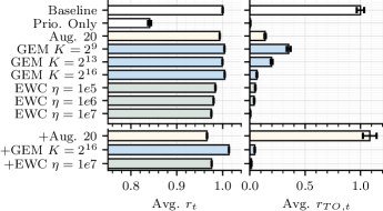
Figure 3: Mean results when using the learned schedulers in evaluation, normalized to the baseline. The left graph shows the performance in overall optimization goal $r_{t}$, where a higher score is better, while the right graph focuses on priority event handling exclusively, where lower is better. Methods are grouped by color, blue denotes the use of GEM, green for EWC, and yellow for schedulers that were not extended but trained on an augmented simulation, all other schedulers are white. Black bars represent the variance. Note that the left graph’s axis is scaled to highlight the relevant area.

While the performance of EWC, GEM may not look overly impressive compared to the augmented simulation, recall that these methods bring further benefits. To emphasize this, we select the Aug. 20 scheduler as well as one choice of EWC, GEM each, unfreeze the NNs, and continue their training on a simulation with ${p_{\text{prio}}=$0$}$, encountering no further priority events. The results after evaluation are displayed in the lower section of Fig. 3, marked with a plus sign. We clearly see the effect of catastrophic forgetting on the Aug. 20 scheduler, which entirely unlearns how to handle priority events. Meanwhile, the EWC scheduler maintains performance on both metrics, while the GEM mechanism can even leverage positive transfer learning, achieving the best overall performance out of all schedulers. Recall further that, as a simulation model comes closer to reality, augmenting a simulation to the desired effect tends to become more and more complex and the augmented simulations data distribution moves further from reality, while EWC, GEM remain at a single control parameter and are trained directly on the true simulation model.

V Conclusion

This paper proposes to decompose a discrete Resource Allocation challenge with Black Swan Events into a two-stage Reinforcement Learning problem, thereby enabling the use of two methods from multi-task learning, Elastic Weight Consolidation (EWC) and Gradient Episodic Memory (GEM). We show that this approach is well able to handle the priority events while offering advantages in robustness over the state-of-the-art approach of changing the training data distribution, at the cost of increased training complexity.

SotA

State of the Art

DoF

Degree of Freedom

3GPP

3rd Generation Partnership Project

RA

Resource Allocation

URLLC

Ultra Reliable and Low Latency Communications

eMBB

enhanced Mobile Broadband

mMTC

massive Machine Type Communication

Tx

Transmit

Rx

Receive

CSIT

Channel State Information at Transmitter

BER

Bit Error Rate

SGD

Stochastic Gradient Descent

MMSE

Minimum Mean Squared Error

DTFT

Discrete Time Fourier Transform

DFT

Discrete Fourier Transform

ZF

Zero Forcings

AWGN

Additive White Gaussian Noise

LOS

Line of Sight

OFDM

Orthogonal Frequency Division Multiplex

OFDMA

Orthogonal Frequency Division Multiplex

NOMA

Non Orthogonal Multiple Access

SISO

Single Input Single Output

SIMO

Single Input Multiple Output

MISO

Multiple Input Single Output

MIMO

Multiple Input Multiple Output

SNR

Signal to Noise Ratio

ML

Machine Learning

DL

Deep Learning

RL

Reinforcement Learning

NN

Neural Network

DQN

Deep Q Network

DDPG

Deep Deterministic Policy Gradient

PPO

Proximal Policy Optimization

EWC

Elastic Weight Consolidation

GEM

Gradient Episodic Memory

NTN

Non Terrestrial Networks

GEO

Geostationary Earth Orbit

LEO

Low Earth Orbit

References

- [1] K. David and H. Berndt, “6G Vision and Requirements: Is There Any Need for Beyond 5G?” IEEE Veh. Technol. Mag., vol. 13, no. 3, pp. 72–80, Sep. 2018.
- [2] NGMN, “6G Drivers and Vision,” https://www.ngmn.org/publications/ngmn-6g-drivers-and-vision.html, 2021, accessed 2022-10-24.
- [3] “Service requirements for the 5G system,” 3GPP, Tech. Rep., 2021.
- [4] G. Cisotto, E. Casarin, and S. Tomasin, “Requirements and enablers of advanced healthcare services over future cellular systems,” IEEE Commun. Mag., vol. 58, no. 3, pp. 76–81, 2020.
- [5] Y. Xu, G. Gui, H. Gacanin, and F. Adachi, “A Survey on Resource Allocation for 5G Heterogeneous Networks: Current Research, Future Trends, and Challenges,” IEEE Commun. Surveys Tuts., vol. 23, no. 2, 2021.
- [6] C. Zhang, P. Patras, and H. Haddadi, “Deep Learning in Mobile and Wireless Networking: A Survey,” arXiv:1803.04311, Jan. 2019.
- [7] M. Roshdi, S. Bhadauria, K. Hassan, and G. Fischer, “Deep Reinforcement Learning based Congestion Control for V2X Communication,” in Proc. IEEE PIMRC. Helsinki, Finland: IEEE, Sep. 2021, pp. 1–6.
- [8] M. Eisen, C. Zhang, L. F. O. Chamon, D. D. Lee, and A. Ribeiro, “Learning Optimal Resource Allocations in Wireless Systems,” IEEE Trans. Signal Process., vol. 67, no. 10, pp. 2775–2790, May 2019.
- [9] A. T. Z. Kasgari, W. Saad, M. Mozaffari, and H. V. Poor, “Experienced Deep Reinforcement Learning with Generative Adversarial Networks (GANs) for Model-Free Ultra Reliable Low Latency Communication,” arXiv:1911.03264, Oct. 2020.
- [10] S. Fujimoto, H. van Hoof, and D. Meger, “Addressing Function Approximation Error in Actor-Critic Methods,” arXiv:1802.09477, Oct. 2018, arXiv: 1802.09477.
- [11] H. Chae, C. M. Kang, B. Kim, J. Kim, C. C. Chung, and J. W. Choi, “Autonomous Braking System via Deep Reinforcement Learning,” arXiv:1702.02302, Apr. 2017.
- [12] L. Pinto, J. Davidson, R. Sukthankar, and A. Gupta, “Robust Adversarial Reinforcement Learning,” arXiv:1703.02702, Mar. 2017.
- [13] J. Kirkpatrick, R. Pascanu, N. Rabinowitz, J. Veness, G. Desjardins, A. A. Rusu, K. Milan, J. Quan, T. Ramalho, A. Grabska-Barwinska, D. Hassabis, C. Clopath, D. Kumaran, and R. Hadsell, “Overcoming catastrophic forgetting in neural networks,” Proc. Natl Acad Sci USA, vol. 114, no. 13, pp. 3521–3526, Mar. 2017.
- [14] S. Gracla, E. Beck, C. Bockelmann, and A. Dekorsy, “Learning resource scheduling with high priority users using deep deterministic policy gradients,” in Proc. IEEE ICC, 2022, pp. 4480–4485.
- [15] ——, “Robust Deep Reinforcement Learning Scheduling via Weight Anchoring,” Accepted for IEEE Commun. Lett., 2022.
- [16] D. Lopez-Paz and M. Ranzato, “Gradient Episodic Memory for Continual Learning,” in Proc. NeurIPS, vol. 30, 2017.
- [17] D. P. Kingma and J. Ba, “Adam: A Method for Stochastic Optimization,” arXiv:1412.6980, 2015.
- [18] A. Achille, M. Rovere, and S. Soatto, “Critical Learning Periods in Deep Networks,” ICLR 2019 Blind Submission, 2019.
- [19] S. Gracla, “Increasing Robustness Against Black Swan Events in Deep Reinforcement Learned Resource Allocation: A Multi-Task Approach,” https://github.com/Steffengra/Anchoring_2, 2022.