Towards Generating Hop-constrained s-t Simple Path Graphs

Abstract.

Graphs have been widely used in real-world applications, in which investigating relations between vertices is an important task. In this paper, we study the problem of generating the $k$-hop-constrained $s$-$t$ simple path graph, i.e., the subgraph consisting of all simple paths from vertex $s$ to vertex $t$ of length no larger than $k$. To our best knowledge, we are the first to formalize this problem and prove its NP-hardness on directed graphs. To tackle this challenging problem, we propose an efficient algorithm named EVE, which exploits the paradigm of edge-wise examination rather than exhaustively enumerating all paths. Powered by essential vertices appearing in all simple paths between vertex pairs, EVE distinguishes the edges that are definitely (or not) contained in the desired simple path graph, producing a tight upper-bound graph in the time cost $\mathcal{O}(k^{2}|E|)$. Each remaining undetermined edge is further verified to deliver the exact answer. Extensive experiments are conducted on $15$ real networks. The results show that EVE significantly outperforms all baselines by several orders of magnitude. Moreover, by taking EVE as a built-in block, state-of-the-art for hop-constrained simple path enumeration can be accelerated by up to an order of magnitude.

1. Introduction

In graph analytics and applications, mining relations between two given vertices is one of the fundamental problems, which helps to make use of connections from a vertex $s$ to another vertex $t$, or to investigate influences or similarities between them based on graph topology (Peng et al., 2019, 2021; Cai and Zheng, 2021; Sun et al., 2021; Wang et al., 2021; Sobrinho and Ferreira, 2020; Cabrera et al., 2020). In this paper, we focus on the problem of $k$-hop-constrained $s$-$t$ simple path graph generation. In many real-life applications, relations between vertices $s$ and $t$ can be captured by enumerating all $s$-$t$ simple paths, where each path is no longer than a user-specific hop constraint $k$ (Peng et al., 2019, 2021). Let us consider the following example.

1.1. Motivation

For graph $G$ in Figure 1(a), all simple paths from vertex $s$ to $t$ with hop constraint $k=4$ are presented in Figure 1(b). The problem of hop-constrained $s$-$t$ simple path enumeration has been well studied, and various novel techniques have been proposed (Rizzi et al., 2014; Peng et al., 2019, 2021; Sun et al., 2021). However, a user may be overwhelmed by the huge number of paths listed. There may be many common vertices and edges in these hop-constrained $s$-$t$ simple paths for large strongly cohesive communities (Peng et al., 2021), as illustrated in Figure 1(b). Such overlaps motivate us to generate a k-hop-constrained $s$-$t$ Simple Path Graph (denoted as $SPG_{k}(s,t)$), a subgraph of input graph $G$, each edge of which is contained in at least a simple path from $s$ to $t$ not longer than $k$. Figure 1(c) is an $s$-$t$ simple path graph with $k=4$ for graph $G$ in Figure 1(a). It captures the main structure of connections between $s$ and $t$, while preserving concision by avoiding repeated vertices and edges in all paths listed in Figure 1(b).

Figure 1. Motivation example

Applications. The problem of $k$-hop-constrained $s$-$t$ simple path graph generation has a wide range of applications, e.g., fraud detection, relation visualization, and accelerating other algorithms.

Fraud Detection. In financial systems, transaction activities can be modeled as a directed graph, where each vertex represents a person or account, and each edge $e(u,v)$ represents a transaction from $u$ to $v$. A simple cycle in such a graph is a strong indication of fraudulent activity or even a financial crime like money laundering (Qiu et al., 2018; Peng et al., 2019, 2021; Sun et al., 2021). For a certain transaction $e(t,s)$, by extracting vertices and edges in all simple cycles containing $e(t,s)$, all fraudsters and fraudulent transactions involved can be identified. In practice, the maximum length is specified for the desired cycles (Sun et al., 2021). Clearly, generating the hop-constrained simple path graph from $s$ to $t$ will immediately produce the target fraudsters and transactions. Similar to previous works (Qiu et al., 2018; Peng et al., 2019, 2021; Sun et al., 2021), non-simple cycles are not considered here, since they may contain other cycles not related to the current edge $e(t,s)$ (i.e., not participating current fraud). Involving them may impose unnecessary repeated punishments and increase downstream workloads (e.g., monitoring and investigation).

Relation Visualization. To discover non-obvious relationships between two entities for decision making and risk reduction (Lohmann et al., 2010), visualizing hop-constrained $s$-$t$ simple path graphs is widely desired in visualization systems, supporting various types of data, such as biological linked data, scientific datasets, and enterprise information networks (Heim et al., 2009; Lohmann et al., 2010; Bäumer et al., 2014; García-Godoy et al., 2011; Peng et al., 2021). For example, given two user-specified nodes $(s,t)$ and some constraints (e.g., path length), RelFinder (Heim et al., 2009; Lohmann et al., 2010) executes SPARQL queries to extract constrained $s$-$t$ simple paths one by one, then displays the $s$-$t$ simple path graph (see Figure 2(a)) instead of listing all paths (e.g., Figure 1(b)). Directly generating the simple path graph not only avoids costly path enumeration, but also provides an initial result which can be further processed for advanced options if required.

Besides the applications above, $k$-hop-constrained $s$-$t$ simple path graph generation can be also used to accelerate other graph algorithms that take simple path graph generation as a built-in block, like (i) hop-constrained simple path enumeration (Rizzi et al., 2014; Peng et al., 2019, 2021; Sun et al., 2021), (ii) quality of service (QoS) routing (Wang and Crowcroft, 1996), and (iii) minimum length-bounded $s$-$t$-cut problem (Baier et al., 2010). They also take vertex pair $(s,t)$ and hop constraint $k$ as input, and edges out of $SPG_{k}(s,t)$ will not be considered for output.

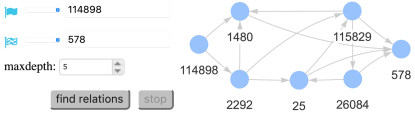
(a) 5-hop simple path graph from Consumer 114898 to 578 on the who-trust-whom online social network (Leskovec et al., 2010)

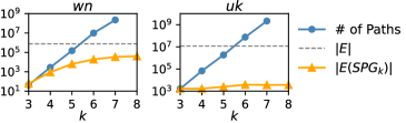
(b) Numbers of edges in $SPG_{k}$ for graphs wn and uk

Figure 2. Illustrations for relation visualization and the growing numbers of edges w.r.t. $k$

1.2. Challenges and Contributions

Challenges. Since a huge search space may be involved when searching from $s$ to $t$ (Peng et al., 2019, 2021), generating $k$-hop-constrained $s$-$t$ simple path graph $SPG_{k}(s,t)$ is computationally expensive. A straightforward solution is to enumerate all $k$-hop-constrained $s$-$t$ simple paths, then put all edges and vertices of these paths together to obtain $SPG_{k}(s,t)$, suffering from the time cost $\mathcal{O}(\delta k|E|)$ where $\delta$ is the number of paths and $|E|$ is the number of edges in $G$ (Peng et al., 2019, 2021; Sun et al., 2021). Since $\delta$ may grow exponentially w.r.t. the number of hops $k$ in real graphs (Peng et al., 2019, 2021), enumerating all paths is far from efficient given the truth that the number of edges in the desired simple path graph is bounded by $|E|$. Take Figure 2(b) as an example which presents the number of edges in $SPG_{k}(s,t)$ and the number of $s$-$t$ simple paths by varying $k$ from 3 to 8 on two graphs from NetworkRepository (Rossi and Ahmed, 2015) (the results are averaged on 1000 random queries for each $k$).

To enhance the efficiency, we need to address three questions.

• Considering the expensive cost of enumerating all the $k$-hop-constrained $s$-$t$ simple paths, is it possible to generate $SPG_{k}(s,t)$ without enumerating all paths?

• Since the problem of generating $SPG_{k}(s,t)$ is NP-hard (as proved in Section 2.1), can we obtain approximate results with high quality in polynomial time?

• As it may need to generate some paths for obtaining the exact $SPG_{k}(s,t)$, how can we accelerate searching process in practice?

To answer these questions, a method named Essential Vertices based Examination (shorted as EVE) is proposed for building the $k$-hop-constrained $s$-$t$ simple path graph $SPG_{k}(s,t)$. Instead of enumerating all paths, EVE examines whether each edge is involved in $SPG_{k}(s,t)$ by introducing essential vertices that summarise common vertices appearing in paths between certain vertex pairs (see Section 3). Powered by essential vertices with a much smaller cost compared to the naive solution above, most failing edges can be filtered out in $\mathcal{O}(k^{2}|E|)$ without enumerating any paths.

To find the essential vertices efficiently, a propagating computation paradigm is developed, in which a forward-looking pruning strategy is exploited to reduce computational costs. Benefiting from essential vertices, each edge can be easily assigned a label indicating whether the edge is definitely (or not) contained in $SPG_{k}(s,t)$, otherwise promising but not verified (called undetermined edges). Thus, an upper-bound graph $SPG^{u}_{k}(s,t)$ (see Section 4) can be acquired. Finally, each undetermined edge will be verified by finding a valid simple path passing the edge. Carefully designed search orders are employed to further accelerate the verification.

Table 1. Summary of notations

Notation	Description
$G$, $G^{r}$	A directed graph and a reversed graph of $G$
$d_{max}$, $d_{avg}$	Maximum and average degree of $G$
$s$, $t$	Source and target vertex for query
$\Delta(s,t)$	Shortest distance from $s$ to $t$
$p(s,t),p^{\ast}(s,t)$	A path and simple path from $s$ to $t$
$V(p),E(p),|p|$	Vertex set, edge set, and length of $p(s,t)$
$P_{k}(s,t)$	All $k$-hop-constrained $s$-$t$ paths
$P_{k}^{*}(s,t)$	All $k$-hop-constrained $s$-$t$ simple paths
$EV_{k}(s,t)$	Essential vertex set of $P_{k}(s,t)$
$EV_{k}^{*}(s,t)$	Essential vertex set of $P_{k}^{*}(s,t)$
$SPG_{k}(s,t)$, $SPG_{k}$	$k$-hop-constrained $s$-$t$ simple path graph
$SPG^{u}_{k}(s,t)$, $SPG^{u}_{k}$	Upper-bound graph of $SPG_{k}$

Contributions. Our contributions are summarised as follows.

• To the best of our knowledge, we are the first to formalize the problem of $k$-hop-constrained $s$-$t$ simple path graph generation, which is motivated by a wide range of applications. We also prove that this problem is NP-hard for directed graphs.

• To address this challenging problem, we develop the paradigm of examining whether an edge is involved in a hop-constrained $s$-$t$ simple path graph powered by essential vertices, instead of exhaustively enumerating all paths.

• We propose an efficient approach, namely EVE, consisting of three components, including propagation for essential vertices, upper-bound graph computation, and verification. The first two steps deliver an upper-bound graph in $\mathcal{O}(k^{2}|E|)$ time. Each undetermined edge is verified with carefully designed search orders.

• We conduct comprehensive experiments on real graphs to compare EVE against baseline methods. EVE significantly outperforms the baselines in terms of time efficiency by up to 4 orders of magnitude. Experimental results also demonstrate the tightness of the computed upper-bound graph which contains less than $0.05\%$ redundant edges for most graphs. Furthermore, PathEnum (Sun et al., 2021) (state-of-the-art for hop-constrained $s$-$t$ simple path enumeration) can be accelerated by up to an order of magnitude powered by the proposed simple path graph.

2. Problem Definition and Overview

We formally define the problem of $k$-hop-constrained $s$-$t$ simple path graph generation, and then give an overview of the proposed EVE. Table 1 lists the frequently-used terms throughout the paper.

2.1. Problem Definition

Let $G=(V,E)$ denote a directed graph, where $V$ is a vertex set and $E\subseteq V\times V$ is an edge set. Let $e(u,v)\in E$ represent a directed edge from vertex $u$ to $v$. The number of vertices and edges are denoted as $|V|$ and $|E|$, respectively. The maximum and average vertex degree are denoted as $d_{max}$ and $d_{avg}$, respectively. Reversing direction of all edges in $G$ leads to a reversed graph, denoted by $G^{r}=(V,E^{r})$.

Given the source vertex $s$ and target vertex $t$, an $s$-$t$ path $p(s,t)=\{s=v_{0},v_{1},\ldots,v_{l-1},v_{l}=t\}$ denotes a directed vertex sequence from $s$ to $t$, where $(v_{i-1},v_{i})\in E$. The vertex set and edge set of path $p(s,t)$ are denoted as $V(p)$ and $E(p)$, and its length is $|p|=l$. A simple path $p^{\ast}(s,t)$ is such a path without duplicate vertices, i.e., $\forall v_{i},v_{j}\in p^{\ast}(s,t)$ s.t. $0\leq i<j\leq l$, $v_{i}\neq v_{j}$. All paths from $s$ to $t$ with length $l\leq k$ is denoted as a set $P_{k}(s,t)=\{p_{1}(s,t),$ $p_{2}(s,t),\ldots,p_{n}(s,t)\}$ where $|p_{i}(s,t)|\leq k$. Similarly, $P_{k}^{*}(s,t)$ denotes all $s$-$t$ simple paths with length $l\leq k$.

Definition 2.1.

($k$-hop-constrained $s$-$t$ Simple Path Graph). Given a graph $G$ and a query $\langle s,t,k\rangle$, the $s$-$t$ simple path graph with hop constraint $k$, denoted as $SPG_{k}(s,t)$=($V^{\ast},E^{\ast}$), is a subgraph of $G$ such that $V^{\ast}=\cup_{p^{\ast}\in P_{k}^{\ast}(s,t)}{V(p^{\ast})}$ and $E^{\ast}=\cup_{p^{\ast}\in P_{k}^{\ast}(s,t)}{E(p^{\ast})}$.

For ease of presentation, $SPG_{k}(s,t)$ can be simplified as $SPG_{k}$. For each edge $e\in E^{\ast}$, there must exist a $k$-hop-constrained $s$-$t$ simple path passing through $e$.

Example 2.2.

For graph $G$ in Figure 1(a), when the hop constraint $k=4$, all $k$-hop-constrained $s$-$t$ simple paths $P_{k}^{\ast}(s,t)$ are shown in Figure 1(b), while $SPG_{k}(s,t)$ is shown in Figure 1(c).

Problem Statement. ($k$-hop-constrained $s$-$t$ Simple Path Graph Generation). For a directed graph $G$, given a query $\langle s,t,k\rangle$, where $s$ and $t$ are two vertices in $G$ ($s\neq t$) and $k$ is the hop constraint, the task is to find the hop-constrained $s$-$t$ simple path graph $SPG_{k}(s,t)$.

2.2. Hardness Analysis

Next, we prove that the problem of generating $SPG_{k}(s,t)$ is NP-hard by introducing Fixed Subgraph Homeomorphism Problem (Fortune et al., 1980). Given a pattern graph $T$ and an input directed graph $G$, a homeomorphism mapping $f$ consists of node-mapping $f^{v}$ and edge-mapping $f^{e}$. $f^{v}$ maps vertices of $T$ to vertices of $G$ and $f^{e}$ maps edges of $T$ to simple paths in $G$, where the involved simple paths in $G$ must be pairwise node-disjoint but allowing shared start and end nodes.

Definition 2.3.

(Fixed Subgraph Homeomorphism Problem, FSH for short) (Fortune et al., 1980). For a fixed pattern graph $T$, given an input directed graph $G$ with node-mapping $f^{v}$ from $T$ to $G$ specified, does $G$ contain a subgraph $G^{*}$ homeomorphic to $T$ ?

Example 2.4.

For the fixed pattern graph $T$ of three vertices and two edges: $\alpha\rightarrow\beta\rightarrow\gamma$, given a directed graph $G$ with a node-mapping specified as $f^{v}_{1}(\alpha)=u$, $f^{v}_{1}(\beta)=x$, and $f^{v}_{1}(\gamma)=z$ in Figure 3(a), the answer to FSH problem is $yes$. It is because there exists a subgraph $G^{*}$ (bold vertices and edges) and $f_{1}$ consisting of $f^{v}_{1}$ and $f^{e}_{1}$ is a homeomorphism mapping.

However, when node-mapping is specified as $f^{v}_{2}(\alpha)=u$, $f^{v}_{2}(\beta)=w$, and $f^{v}_{2}(\gamma)=z$, the answer is $no$. As shown in Figure 3(b), $f^{e}_{2}$ is not a homeomorphism edge-mapping, since path $u\rightarrow v\rightarrow x\rightarrow w$ and $w\rightarrow x\rightarrow y\rightarrow z$ share the common vertex $x$.

When the pattern graph $T$ is fixed to be a path with two edges connecting three distinct vertices (i.e., $\alpha\rightarrow\beta\rightarrow\gamma$), it can be proved that determining whether $T$ is subgraph homeomorphic to $G$ under a node mapping $f^{v}$ is NP-complete (Fortune et al., 1980).

Theorem 2.5.

The $k$-hop-constrained $s$-$t$ simple path graph generation problem for directed graphs is NP-hard.

Proof.

For the fixed pattern graph $T$: $\alpha\rightarrow\beta\rightarrow\gamma$, the FSH problem can be reduced to k-hop-constrained $s$-$t$ simple path graph generation in $\mathcal{O}(|V|^{2})$ time. Specifically, given a directed graph $G$ with a node-mapping $f^{v}(\alpha)=s$, $f^{v}(\beta)=r$, and $f^{v}(\gamma)=t$ where $s$, $r$, and $t$ are three distinct vertices in $G$, the FSH problem can be solved by generating $SPG_{k}(s,t)$ for $k=1,2,\cdots,|V|-1$.

(1) If $\exists k$ s.t. $r\in V(SPG_{k}(s,t))$, there exists a simple path $p^{\ast}$ from $s$ to $t$ through $r$. $p^{\ast}$ can be split into node-disjoint simple paths $p^{\ast}(s,r)$ and $p^{\ast}(r,t)$. Hence, the answer to the FSH problem is $yes$.

(2) If $\forall k$, $r\not\in V(SPG_{k}(s,t))$, there does not exist node-disjoint simple paths $p^{\ast}(s,r)$ and $p^{\ast}(r,t)$. Otherwise, joining $p^{\ast}(s,r)$ and $p^{\ast}(r,t)$ together will obtain a simple path $p^{\ast}(s,t)$ passing through $r$. Hence, the answer to the FSH problem is $no$.

Thus, if the $k$-hop-constrained $s$-$t$ simple path graph generation can be solved in polynomial time, the FSH problem will be solved in polynomial time too, which contradicts its NP-completeness. ∎

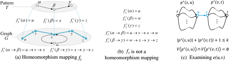
Figure 3. Illustration for fixed subgraph homeomorphism problem and Oberservation 2.1

We also discuss the hardness of generating $SPG_{k}(s,t)$ when $k$ is much smaller than $|V|$.

Theorem 2.6.

For any constant $\epsilon\in(0,1)$, the problem of generating $SPG_{k}(s,t)$ given $k=|V|^{\epsilon}$ on directed graphs is NP-hard.

Proof.

For each graph $G(V,E)$ of the FSH problem, we construct a graph $G^{\prime}(V^{\prime},E^{\prime})$ by adding $(|V|^{\frac{1}{\epsilon}}-|V|)$ isolated vertices to $G$ such that $|V^{\prime}|=|V|^{\frac{1}{\epsilon}}$ and $E^{\prime}=E$. Similar to the proof of Theorem 2.5, we can generate $SPG_{k}(s,t)$ over graph $G^{\prime}$ with $k=|V^{\prime}|^{\epsilon}$ and return $yes$ for the FSH problem iff $r\in V(SPG_{k}(s,t))$. Since adding $(|V|^{\frac{1}{\epsilon}}-|V|)$ isolated vertices costs polynomial time, if we can generate $SPG_{k}(s,t)$ over $G^{\prime}$ given $k=|V^{\prime}|^{\epsilon}$ in polynomial time, the FSH problem will be solved in polynomial time too, which contradicts the NP-completeness of the FSH problem. ∎

Theorem 2.7.

The problem of $k$-hop-constrained $s$-$t$ simple path graph generation is fixed-parameter tractable (FPT).

Proof.

Let us consider the Directed k-(s, t)-Path Problem that decides whether there is an $s$-$t$ simple path of length $k$ in a directed graph $G$ (Fomin et al., 2018). Directed k-(s, t)-Path Problem is fixed-parameter tractable and can be solved in $\mathcal{O}(2^{\mathcal{O}(k)}E)$ (Alon et al., 1995) as a generalization of $k$-path, i.e., it can be solved in polynomial time for $k=\log|V|$.

The solution to Directed k-(s, t)-Path Problem can be also used to build $SPG_{k}(s,t)$. Specifically, $SPG_{k}(s,t)$ can be obtained by checking each edge $e(u,v)$. It holds that $e(u,v)\in SPG_{k}(s,t)\Leftrightarrow\exists$ a simple path $p^{\ast}$ through $e(u,v)$ s.t. $|p^{\ast}|\leq k$. For each edge $e(u,v)$, we construct an auxiliary graph $G^{\prime}(V^{\prime},E^{\prime})$ by inserting a new vertex into every edge in $G$ (i.e., splitting each edge of $G$ into two edges connected by a new vertex) except $e(u,v)$, resulting in $|V^{\prime}|=|V|+|E|-1$ and $|E^{\prime}|=2|E|-1$. Next, we invoke the solver of Directed $k^{\prime}$-(s, t)-Path Problem for $k^{\prime}=1,3,5,\cdots,2k-1$, where $k^{\prime}$ is an odd number. Then we have: $\exists k^{\prime}$ s.t. there exists an $s$-$t$ simple path $q^{\ast}$ of length $k^{\prime}$ in $G^{\prime}$ $\Leftrightarrow\;\exists$ an $s$-$t$ simple path $p^{\ast}$ of length $l=\frac{k^{\prime}+1}{2}\leq k$ passing through $e(u,v)$ in $G$. Proof is trivial by noticing that each of the other edges in $G$ is split into two edges in $G^{\prime}$, and any $s$-$t$ simple path of odd length in $G^{\prime}$ must pass through $e(u,v)$.

The reduction above takes the $\mathcal{O}(k|E|^{2})$ time. Since Directed k-(s, t)-Path Problem is FPT, generating $SPG_{k}(s,t)$ is also FPT. ∎

Notice that though the FPT algorithm mentioned in the proof above is theoretically feasible, it has a significant failure rate as shown in extensive experiments (Yeh et al., 2012).

2.3. Overview of Our Approach

Enumerating all $k$-hop-constrained $s$-$t$ simple paths with naive DFS, leading to the time cost $\mathcal{O}(|V|^{k})$. It is still computationally expensive even equipped with state-of-the-art algorithms for path enumeration. To efficiently generate $SPG_{k}(s,t)$, we focus on the question: Given an edge $e(u,v)$, does it belong to $SPG_{k}(s,t)$?

Observation 2.1.

$e(u,v)\in SPG_{k}(s,t)\Leftrightarrow\exists\;p^{\ast}(s,u),p^{\ast}(v,t)$ s.t. (1) $|p^{\ast}(s,u)|+|p^{\ast}(v,t)|+1\leq k$ and (2) $V(p^{\ast}(s,u))\cap V(p^{\ast}(v,t))=\emptyset$.

As illustrated in Figure 3(c), Observation 2.1 holds since any desired path $p^{\ast}(s,t)$ through $e(u,v)$ can be decomposed into $p^{\ast}(s,u)$, $e(u,v)$, and $p^{\ast}(v,t)$ s.t. conditions (1) and (2) are satisfied. By iterating each edge $e(u,v)$ and each pair $(p^{\ast}(s,u),p^{\ast}(v,t))$ for checking the conditions (1) and (2), we can find out all edges of $SPG_{k}$. However, computing and iterating all pairs of $p^{\ast}(s,u)$ and $p^{\ast}(v,t)$ is still unacceptable in both time and space cost.

Intuitively, by ensuring shortest distances $\Delta(s,u)+\Delta(v,t)+1\leq k$, it is easy to determine whether an edge $e(u,v)$ satisfies condition (1). However, there are still many failing edges $e(u,v)$ caused by some vertices appearing in both $p^{\ast}(s,u)$ and $p^{\ast}(v,t)$ (i.e., do not satisfy condition (2)). Thus, we introduce the concept of Essential Vertices (formally defined in Definition 3.1) for vertices appearing in all $k$-hop-constrained simple paths $p^{\ast}(s,u)$ (or $p^{\ast}(v,t)$), denoted by $EV^{\ast}_{k}(s,u)$ (or $EV^{\ast}_{k}(v,t)$). Take edge $e(u,v)$ in Figure 4(a) as an example, $EV^{\ast}_{k}(s,u)=EV^{\ast}_{k}(v,t)=\{x\}$ when $k=6$ since vertex $x$ lies on all $p^{\ast}(s,u)$ and $p^{\ast}(v,t)$. Thus, $EV^{\ast}_{k}(s,u)\cap EV^{\ast}_{k}(v,t)\neq\emptyset$, concluding that $e(u,v)\not\in SPG_{k}(s,t)$. In this paper, we prove that edge $e(u,v)\not\in SPG_{k}(s,t)$ if $EV_{k_{f}}^{*}(s,u)\cap EV_{k_{b}}^{*}(v,t)\neq\emptyset$ for $\forall k_{f},k_{b}$ s.t. $k_{f}+k_{b}+1\leq k$ (see Theorem 3.4), which helps to effectively identify failing edges in practice. Experiments show that when $k=6$, among edges only satisfying condition (1), there are about $30\%$ redundant edges not in $SPG_{k}$ (averaged on 1000 random queries for all datasets in Table 2). After filtering with essential vertices, there are only about $0.1\%$ redundant edges left.

We summarise our proposed method EVE in three phases which avoids the expensive cost of iterating all pairs of $p^{\ast}(s,u)$ and $p^{\ast}(v,t)$ for examining each edge $e(u,v)$, as shown in Figure 4(b).

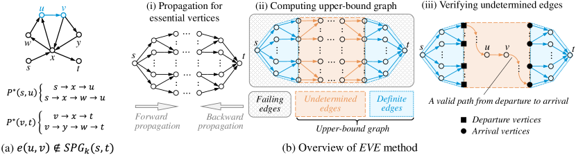
Figure 4. Illustration for general ideas of the EVE method

(1) Propagation for Essential Vertices. To obtain $EV^{\ast}_{k}(s,w)$ and $EV^{\ast}_{k}(w,t)$ for any vertex $w$, we conduct forward propagation from $s$ and backward propagation from $t$, where essential vertices are propagated layer by layer. To further reduce unnecessary propagating cost, we develop forward-looking pruning strategy that takes the shortest distance from $s$ to $u$ (resp. $\Delta(s,u)$) and the shortest distance from $v$ to $t$ (resp. $\Delta(v,t)$) into consideration, ensuring that $EV^{\ast}_{l}(s,w)$ and $EV^{\ast}_{l}(w,t)$ computed in the current propagation step $l$ will be used. Adaptive bi-directional search is exploited to efficiently obtain such shortest distances before propagation.

(2) Computing upper-bound graph. All edges are categorized into three sets including failing edges, undetermined edges, and definite edges. Specifically, failing edges are found and filtered out based on essential vertices by Theorem 3.4, while an upper-bound graph $SPG_{k}^{u}$ can be obtained from the remaining edges (see Section 4.1). Furthermore, each edge in $SPG_{k}^{u}$ will be distinguished as a definite edge or an undetermined edge (see Section 4.2).

(3) Verifying Undetermined Edges. Departures and arrivals (formally defined in Section 5.1) are computed on $SPG_{k}^{u}(s,t)$, which are boundary vertices connecting undetermined and definite edges. For each undetermined edge $e(u,v)$, DFS-oriented search is conducted to find a valid simple path from departure to arrival through $e(u,v)$ by Theorem 5.6. If such valid path exists, $e(u,v)\in SPG_{k}(s,t)$. With carefully designed searching orders, verification process is further accelerated.

When $k\leq 4$, the upper-bound graph $SPG^{u}(s,t)$ computed above always equals $SPG_{k}(s,t)$ (Theorem 4.8), indicating no false-positive edges will be produced. When $k\leq 5$, it only takes $\mathcal{O}(|E|)$ time and space for generating the exact $SPG_{k}(s,t)$ (Theorem 5.9).

3. Essential Vertex Computation

We first present the principle of introducing essential vertices (Section 3.1). To compute essential vertices, a propagation based algorithm is proposed (Section 3.2). To speed up the computation, we propose a forward-looking pruning strategy (Section 3.3).

3.1. Essential Vertices

As discussed in Section 2.3, Observation 2.1 abstracts the existence of a path $p^{\ast}(s,t)$ through $e(u,v)$ by checking the constraints for each edge individually. This insight has the advantage of substantially avoiding edges’ repetitive visits, but validating each edge still demands significant overhead. Thus, greedy or pruning methods should be introduced to minimize edge-wise verification.

Pruning Principle. When $P_{k-1}^{\ast}(s,u)\neq\emptyset$ and $P_{k-1}^{\ast}(v,t)\neq\emptyset$, edge $e(u,v)$ cannot be contained in $SPG_{k}(s,t)$ iff: $\forall p^{\ast}(s,u)\in P_{k-1}^{\ast}(s,u)$, $p^{\ast}(v,t)\in P_{k-1}^{\ast}(v,t)$ s.t. $|p^{\ast}(s,u)|+|p^{\ast}(v,t)|<k$, $V(p^{\ast}(s,u))\cap$ $V(p^{\ast}(v,t))\neq\emptyset$. In other words, though it is possible to form a path of length $|p^{\ast}(s,t)|\leq k$, duplicate vertices are inevitable in each of such paths. Thus, it provides opportunities for identifying the case $e(u,v)\notin SPG_{k}(s,t)$ when $P_{k-1}^{\ast}(s,u)$ and $P_{k-1}^{\ast}(v,t)$ satisfy certain features. We extract the key features associated with the vertices, named as essential vertices.

Definition 3.1.

(Essential Vertices). Given query vertices $s$ and $t$ in $G$, essential vertices for $P_{l}^{\ast}(s,u)$ are denoted as $EV_{l}^{*}(s,u)$, i.e., the set of vertices that are contained in all simple paths not passing through $t$ in $P_{l}^{*}(s,u)$. Formally, we have

(1) $$EV_{l}^{\ast}(s,u)=\bigcap\limits_{p_{i}^{\ast}\in P_{l}^{\ast}(s,u)\;s.t.\;t\not\in V(p_{i}^{\ast})}V(p_{i}^{\ast}).$$

The vertices in $EV_{l}^{*}(s,u)$ are essential, since to form a simple path $p^{\ast}(s,t)$, there will be no $p^{\ast}(s,u)$ with $\lvert p^{\ast}(s,u)\rvert\leq l$ if all vertices in $EV_{l}^{*}(s,u)$ are removed. Similarly, we have

(2) $$EV_{l}^{\ast}(v,t)=\bigcap\limits_{p_{i}^{\ast}\in P_{l}^{\ast}(v,t)\;s.t.\;s\not\in V(p_{i}^{\ast})}V(p_{i}^{\ast}).$$

Example 3.2.

For graph $G$ in Figure 1(a), essential vertices $EV_{l}^{\ast}(s,\cdot)$ and $EV_{l}^{\ast}(\cdot,t)$ for $1\leq l\leq 6$ are shown in Figure 5(a)-(b). Take vertex $b$ as an example, $P_{2}^{\ast}(s,b)=\{\{s,c,b\}\}$, $P_{3}^{\ast}(s,b)=\{\{s,c,b\},\{s,a,h,b\},$ $\{s,a,c,b\}\}$. Thus, $EV_{2}^{\ast}(s,b)=\{s,c,b\}$ and $EV_{3}^{\ast}(s,b)=\{s,b\}$.

Based on $EV_{l}^{*}(s,u)$ and $EV_{l}^{\ast}(v,t)$, we can determine which edges can be definitely excluded from $SPG_{k}(s,t)$ by Theorem 3.4.

Lemma 3.3.

If $e(u,v)\in SPG_{k}(s,t)$, it holds that $\exists\;EV^{\ast}_{k_{f}}(s,u)$ and $\exists\ EV^{\ast}_{k_{b}}(v,t)$ s.t. (1) $k_{f}+1+k_{b}\leq k$, and (2) $EV_{k_{f}}^{*}(s,u)\cap EV_{k_{b}}^{*}(v,t)=\emptyset$; but not necessarily the reverse.

Proof.

Sufficiency. As $e(u,v)\in SPG_{k}(s,t)$, there must exist a simple path $p^{*}(s,u)$ whose length is $k_{f}$ and $p^{*}(v,t)$ whose length is $k_{b}$ subject to the condition that $k_{f}+k_{b}+1\leq k$ and $V(p^{\ast}(s,u))\cap V(p^{\ast}(v,t))=\emptyset$. Meanwhile, $EV^{\ast}_{k_{f}}(s,u)\subseteq V(p^{*}(s,u))$ and $EV^{\ast}_{k_{b}}(v,t)\subseteq V(p^{*}(v,t))$. Therefore, $EV^{\ast}_{k_{f}}(s,u)\cap EV^{\ast}_{k_{b}}(v,t)=\emptyset$.
Necessity. Consider edge $e(b,a)$ as a counterexample in Figure 1(a). If $k=7$, for $k_{f}=3\land k_{b}=2$ satisfying condition (1), $EV_{3}^{\ast}(s,b)=\{s,b\}$ and $EV_{2}^{\ast}(a,t)=\{a,c,t\}$. Thus, $EV_{3}^{\ast}(s,b)\cap EV_{2}^{\ast}(a,t)=\emptyset$ and condition (2) also holds. However, no simple path from $s$ to $t$ passing $e(b,a)$ can be formed. Thus, the necessity is not established. ∎

Theorem 3.4.

If $\forall 0\leq k_{f},k_{b}\leq k-1$ s.t. $k_{f}+1+k_{b}\leq k$, we have (1) $EV_{k_{f}}^{\ast}(s,u)$ or $EV_{k_{b}}^{\ast}(v,t)$ does not exist (i.e., there is no simple path $p^{\ast}(s,u)$ or $p^{\ast}(v,t)$ of length no larger than $k_{f}$ or $k_{b}$, respectively); or (2) $EV_{k_{f}}^{\ast}(s,u)\cap EV_{k_{b}}^{\ast}(v,t)\neq\emptyset$, then $e(u,v)\notin SPG_{k}(s,t)$.

The proof of Theorem 3.4 is omitted since it is the contrapositive statement of Lemma 3.3. Hence, we can prune as many edges as possible to achieve a practically tight upper bound of the desired $k$-hop-constrained $s$-$t$ simple path graph (for more details please refer to Section 4). Thus, overall time cost can be greatly reduced.

3.2. Propagating Computation

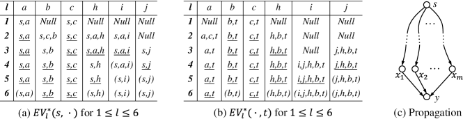
Figure 5. Illustrations for essential vertex computation

Directly computing essential vertices based on the definition is challenging. Specifically, to compute $EV^{\ast}_{l}(s,u)$, all simple paths $p^{\ast}(s,u)$ with $\lvert p^{\ast}(s,u)\rvert\leq l$ have to be enumerated, and their vertices need to be intersected. To address the problem, we propose an efficient propagating computation for essential vertices, which works on the fact that intersecting all simple paths’ vertices is equivalent to intersecting all paths’ vertices (the correctness is guaranteed by Theorem 3.5). Similar to $EV^{*}_{l}(s,u)$, let $EV_{l}(s,u)$ denote the intersection of vertices of all paths not passing through $t$ in $P_{l}(s,u)$. Formally,

(3) $$EV_{l}(s,u)=\bigcap\limits_{p_{j}\in P_{l}(s,u)\;s.t.\;t\not\in V(p_{j})}V(p_{j}).$$

The basic principle is that the essential vertices of $EV_{l}(s,y)$ can be computed based on the essential vertices of $y$’s incoming neighbors. Note that for ensuring $t\not\in V(p_{j})$ in Equation (3), vertex $t$ will never be visited when computing $EV_{l}(s,y)$. Let $In(y)$ denote the incoming neighbors of vertex $y$. Formally, the propagating computation follows the recursive formula below.

(4) $$EV_{l}(s,y)=\bigcap_{x_{i}\in In(y)}\left(EV_{l-1}(s,x_{i})\cup\{y\}\right)$$

Intuitions of Equation (4): Any path $p(s,y)$ with length $|p(s,y)|\leq l$ is composed of two parts, i.e., a path $p(s,x_{i})$ and an edge $e(x_{i},y)$, where $x_{i}\in In(y)$. Taking Figure 5(c) as an example, suppose $x_{1}$, $x_{2}$, $\ldots$, $x_{m}$ are all the in-neighbors of $y$ s.t. $P_{l-1}(s,x_{i})\neq\emptyset$ ($1\leq i\leq m$). A path $p(s,y)$ with $\lvert p(s,y)\rvert\leq l$ must pass through an edge $e(x_{i},y)$. Given essential vertices $EV_{l-1}(s,x_{i})$ for paths $p(s,x_{i})$ with length $|p(s,x_{i})|\leq l-1$, all the essential vertices from $s$ to $y$ through $e(x_{i},y)$ within length $l$ are $EV_{l-1}(s,x_{i})\cup\{y\}$. Thus, intersecting essential vertices through $e(x_{i},y)$ for all $x_{i}\in In(y)$ leads to $EV_{l}(s,y)$.

Propagation is terminated when $l>k-1$, since only $EV^{\ast}_{l}(s,u)$ for $l\leq k-1$ are required in Theorem 3.4. To propagate essential vertices through edges within ($k-1$)-hop edges from $s$, we introduce an algorithm Forward Propagation (see Algorithm 1). It first initializes all essential vertex sets in line 3, then stimulates the process of path generation from $s$ and maintains a queue called $Frontier$. For a certain length $l$, the algorithm visits out-neighbors $y\in Out(x)$ for vertices $x$ in the $Frontier$, and intersects $EV_{l}(s,y)$ with $EV_{l-1}(s,x)\cup\{y\}$ in lines 8-12. From another prospective, for each vertex $y$ explored in layer $l$, the algorithm propagates the set of essential vertices from its in-neighbors by Equation (4). Note that in line 14, if vertex $u$ has not been visited in current layer $l$, $EV_{l}(s,u)$ can inherit vertices from $EV_{l-1}(s,u)$, since paths within $l-1$ hops are not longer than $l$.

Algorithm 1 Forward Propagation

1:Hop constraint $k$, source vertex $s$, and graph $G=(V,E)$.

2:$EV_{l}(s,y)$ for $y\in V$ and $1\leq l<k$.

3:$EV_{l}(s,u)\leftarrow null$ for each $u\in V$ where $l=0$ to $k-1$

4:$Frontier\leftarrow\{s\}$; $EV_{0}(s,s)\leftarrow\{s\}$

5:for $l=1$ to $k-1$ do

6:    $nextFrontier\leftarrow\emptyset$

7:    for $x$ in $Frontier$ do

8:        for $y$ in $Out(x)$ s.t. $y\neq s$ $\land$ $y\neq t$ do

9:           if $EV_{l}(s,y)=null$ then

10:               $EV_{l}(s,y)\leftarrow EV_{l-1}(s,x)\cup\{y\}$

11:           else

12:               $EV_{l}(s,y)\leftarrow EV_{l}(s,y)\cap(EV_{l-1}(s,x)\cup\{y\})$            

13:           Add $y$ to $nextFrontier$             

14:    $EV_{l}(s,u)\leftarrow EV_{l-1}(s,u)$ for each $u\in V$ if $EV_{l}(s,u)=null$

15:    $Frontier\leftarrow nextFrontier$

To compute essential vertices $EV_{l}^{\ast}(v,t)$ of any length $l$ from every vertex $v$ to $t$, we run this algorithm on the reversed graph $G^{r}$, taking $t$ as the source vertex. This process is called Backward Propagation. Next, we show that Algorithm 1 is correct as $EV_{l}(s,u)=EV_{l}^{*}(s,u)$.

Theorem 3.5.

$\forall$ vertex pair $(s,u)$ and $l\geq 1$, $EV_{l}(s,u)=EV_{l}^{\ast}(s,u)$.

Proof.

When $P_{l}^{\ast}(s,u)\subset P_{l}(s,u)$, we have $P_{l}(s,u)\neq\emptyset$ and there exists a path $p(s,u)\in P_{l}(s,u)$ reusing vertices. We can always find a repeatedly used vertex $x$ that taking out the first $x$ in the path (denoted as $x_{1}$) and the last one (denoted as $x_{n}$), such that the path $p(s,u)=\{s,\ldots,$ $x_{1},\ldots,x_{n},\ldots,u\}$ split by $x_{1}$ and $x_{n}$ follows the constraint that no vertex $y$ exists both in $p(s,x_{1})$ and $p(x_{n},u)$. If we combine $p(s,x_{1})$ with $p(x_{n},u)$, the new path is a path $p^{x}(s,u)$ from $s$ to $u$ with no vertex reused, whose length $|p^{x}(s,u)|<|p(s,u)|\leq l$. As $V(p^{x}(s,u))\subseteq V(p(s,u))$, it holds that $\forall p\in P_{l}(s,u)$, there must exist a simple path $p^{\ast}\in P_{l}^{\ast}(s,u)\subset P_{l}(s,u)$ satisfying $V(p^{\ast})\cap V(p)=V(p^{\ast})$. Thus, $EV_{l}(s,u)=\bigcap_{p_{j}\in P_{l}(s,u)\;s.t.\;t\not\in V(p_{j})}V(p_{j})=\bigcap_{p_{i}^{\ast}\in P_{l}^{\ast}(s,u)\;s.t.\;t\not\in V(p_{i}^{\ast})}V(p_{i}^{\ast})=EV_{l}^{\ast}(s,u)$. ∎

3.3. Forward-looking Pruning Strategy

In forward propagation, essential vertices are computed for every vertex $u$ satisfying $\Delta(s,u)<k$. However, not all $EV_{l}^{\ast}(s,u)$ will be useful for filtering unpromising edges. Intuitively, for any vertex $u$ s.t. $\Delta(s,u)+\Delta(u,t)>k$, computing $EV^{\ast}_{l}(s,u)$ is meaningless due to length constraint. Moreover, even for vertex $u$ satisfying $\Delta(s,u)+\Delta(u,t)\leq k$, unnecessary computation can also be avoided.

Theorem 3.6.

If $l+\Delta(u,t)>k$, computing $EV_{l}^{\ast}(s,u)$ contributes nothing to concluding any edge $e(u,v)\not\in SPG_{k}(s,t)$ by Theorem 3.4.

Proof.

For edge $e(u,v)$, if $l+\Delta(u,t)>k$, there does not exist $EV^{\ast}_{k_{b}}(v,t)$ s.t. $l+1+k_{b}\leq k$. Thus, statement (1) in Theorem 3.4 holds when $k_{f}=l$. If such $EV_{l}^{\ast}(s,u)$ are not computed (i.e., not exist), statement (1) still holds when $k_{f}=l$. ∎

Based on Theorem 3.6, we develop a forward-looking pruning strategy which concerns the steps needed for reaching $t$ in future. Specifically, $l+\Delta(y,t)\leq k$ is required when propagating from vertex $x$ to $y$ at $l^{th}$ step. In other words, line 8 of Algorithm 1 is changed to: for $y$ in $Out(x)$ s.t. $y\neq s$ $\land$ $y\neq t$ $\land$ $l+\Delta(y,t)\leq k$. Note that when $l+\Delta(y,t)>k$, $y$ will not be added to $nextFrontier$ in line 13 for exploring its out-neighbors. It is because $y$ has no descendants $y^{\prime}$ at any step $l^{\prime}$ ($l^{\prime}>l$) satisfying $l^{\prime}+\Delta(y^{\prime},t)\leq k$, otherwise $l+\Delta(y,t)\leq l+(l^{\prime}-l+\Delta(y^{\prime},t))\leq k$.

Example 3.7.

Given graph $G$ (Figure 1(a)) and $k=7$, those essential vertices in parenthesis in Figure 5(a) will not be computed. For example, $EV^{\ast}_{l}(s,i)$ for $l>3$ can be omitted since $\Delta(i,t)=4$.

In practice, when $EV^{\ast}_{l}(s,u)$ are the same for different $l$, we only store the first one since the others can refer to it. For instance, those underlined essential vertices in Figure 5(a) can be omitted. Similarly, time and space cost of backward propagation can also be reduced. Note that shortest distances $\Delta(s,y)$ and $\Delta(y,t)$ should be computed before starting propagation. Intuitively, we can conduct forward BFS from $s$ and backward BFS from $t$, but better solutions exist.

We can only compute distances for vertices $y$ satisfying $\Delta(s,y)+\Delta(y,t)\leq k$ and assign $+\infty$ for the other vertices $w$, since $l+\Delta(w,t)\geq\Delta(s,w)+\Delta(w,t)>k$ will stop forward propagation for $w$ at step $l$. As shown in Figure 6(a), bi-directional BFS (Goldberg and Harrelson, 2005; Wang et al., 2021) explores forward from $s$ and backward from $t$ with equal depth, then continues forward (resp. backward) search for the remaining steps over edges explored backward (resp. forward). To improve the performance, we can use Adaptive Bi-directional Search (Holzer et al., 2005; Ahuja et al., 1993), in which forward and backward BFS start simultaneously. It adaptively explores in the direction having a smaller frontier at each step, until the total depth reaches $k$.

Time Complexity of Computing Essential Vertices. To compute essential vertices, adaptive bi-directional search first obtains shortest distances in $\mathcal{O}(\lvert E\rvert)$ time. Then Algorithm 1 initializes $EV_{l}(s,u)$ for all vertices $u$ with $0\leq l<k$. For each $l$, it updates $EV_{l}(s,y)$ for all out-neighbors $y$ of vertices $x$ in the frontier by intersecting $EV_{l-1}(s,x)\cup\{y\}$ with $EV_{l}(s,y)$, which needs at most $\lvert E\rvert$ intersections since there are $\lvert E\rvert$ edges in the graph. In each intersection, each essential vertices set contains at most $l+1$ vertices. Thus, total time complexity is $\mathcal{O}(k^{2}\lvert E\rvert)$.

Space Complexity of Computing Essential Vertices. Adaptive bi-directional search maintains two BFS frontiers requiring $\mathcal{O}(\lvert V\rvert)$ complexity. Essential vertices sets from $s$ and to $t$ are maintained for each vertex of all length $l$ ($0\leq l<k$). For each length, up to $l$ essential vertices exist. Thus, total space complexity is $\mathcal{O}(k^{2}\lvert V\rvert)$.

4. Essential Vertex based Upper Bound

As shown in step (ii) of the overview (Figure 4(b)), we divide all edges in $G$ into three groups: Failing edges, which are definitely not in $SPG_{k}(s,t)$, labeled as “0”; Undetermined edges, which are a promising edge in $SPG_{k}(s,t)$ but not verified, labeled as “1”; Definite edges, which are definitely contained in $SPG_{k}(s,t)$, labeled as “2”. Section 4.1 focuses on ruling out failing edges to form an upper-bound graph, while definite edges are identified in Section 4.2.

4.1. Computing the Upper-Bound Graph

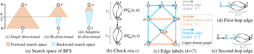
Figure 6. Illustrations for BFS search space and edge labeling

As proved in Theorem 2.5, generating the $k$-hop-constrained $s$-$t$ simple path graph is an NP-hard problem. Therefore, it motivates us to find an upper bound of the target path graph to narrow down the search space for computing $SPG_{k}(s,t)$.

As illustrated in Figure 6(b), according to Theorem 3.4, for each edge $e(u,v)$ we can iterate all pairs of integers ($k_{f}$, $k_{b}$) s.t. $k_{f}+1+k_{b}\leq k$. We can conclude that $e(u,v)\not\in SPG_{k}(s,t)$ if none of the pairs ($k_{f}$, $k_{b}$) satisfies the constraints that (1) $EV_{k_{f}}^{\ast}(s,u)$ and $EV_{k_{b}}^{\ast}(v,t)$ exist; and (2) $EV_{k_{f}}^{\ast}(s,u)\cap EV_{k_{b}}^{\ast}(v,t)=\emptyset$. Otherwise, it contributes to forming an upper-bound graph of $SPG_{k}(s,t)$.

Definition 4.1.

(Upper-bound graph of $SPG_{k}(s,t)$). An upper-bound graph of $SPG_{k}(s,t)$, denoted as $SPG_{k}^{u}(s,t)=(V^{u},E^{u})$, is a subgraph of $G$ such that: $e(u,v)\in E^{u}\Leftrightarrow$ $\exists\;EV^{\ast}_{k_{f}}(s,u)$ and $\exists\ EV^{\ast}_{k_{b}}(v,t)$ s.t. (1) $k_{f}+1+k_{b}\leq k$, and (2) $EV_{k_{f}}^{*}(s,u)\cap EV_{k_{b}}^{*}(v,t)=\emptyset$.

To form $SPG_{k}^{u}(s,t)$, we iterate each edge $e(u,v)$ to check whether it is contained in $SPG_{k}^{u}(s,t)$ based on Definition 4.1. Note that the edges out of adaptive bi-directional search space (Section 3.3) are not considered, since they cannot satisfy distance constraint.

Example 4.2.

Given the graph $G$ in Figure 1(a) and $k=7$, the upper-bound graph $SPG_{k}^{u}(s,t)$ is shown in Figure 6(c). Take edge $e(i,j)$ as an example. Since for $k_{f}=2$ and $k_{b}=3$ we have $EV^{\ast}_{k_{f}}(s,i)=\{s,a,i\}$ and $EV^{\ast}_{k_{b}}(j,t)=\{j,h,b,t\}$ according to Figure 5(a)-(b). $EV^{\ast}_{k_{f}}(s,i)\cap EV^{\ast}_{k_{b}}(j,t)=\emptyset$ leads to $e(i,j)\in SPG^{u}_{k}$. In contrast, edge $e(b,j)$ is a failing edge since $EV^{\ast}_{k_{b}}(j,t)=\{j,h,b,t\}$ for $k_{b}\geq 3$, but $b\in EV^{\ast}_{k_{f}}(s,b)$ for $k_{f}\geq 2$ and $EV^{\ast}_{k_{f}}(s,b)\cap EV^{\ast}_{k_{b}}(j,t)\neq\emptyset$.

When examining each edge $e(u,v)$, it is unnecessary to enumerate all integer pairs ($k_{f}$, $k_{b}$) s.t. $k_{f}+1+k_{b}\leq k$. Actually, we iterate $k_{f}$ from $0$ to $k-1$ and check requirements over $EV^{\ast}_{k_{f}}(s,u)$ and $EV^{\ast}_{k_{b}}(v,t)$ with $k_{b}=k-k_{f}-1$. It is because checking $k_{b}=k-k_{f}-1$ already covers the examination for all $k_{b}<k-k_{f}-1$. The correctness is guaranteed by Theorem 4.3.

Theorem 4.3.

For a certain $k_{f}$ ($0\leq k_{f}\leq k-1$) and $k_{b}=k-k_{f}-1$, if $EV_{k_{b}}^{\ast}(v,t)$ does not exist, $EV_{l}^{\ast}(v,t)$ will not exist for any $l<k_{b}$. And if $EV_{k_{f}}^{\ast}(s,u)\cap EV_{k_{b}}^{\ast}(v,t)\neq\emptyset$, $EV_{k_{f}}^{\ast}(s,u)\cap EV_{l}^{\ast}(v,t)\neq\emptyset$.

Proof.

Since $P_{k}^{\ast}(v,t)$ denotes all $k$-hop-constrained $s$-$t$ simple paths, $\forall l<k_{b}$, $P_{l}^{\ast}(v,t)\subseteq P_{k_{b}}^{\ast}(v,t)$, and $EV_{k_{b}}^{\ast}(v,t)\subseteq EV_{l}^{\ast}(v,t)$. If $EV_{k_{b}}^{\ast}(v,t)$ does not exist, $P_{k_{b}}^{\ast}(v,t)=\emptyset$. Thus, $P_{l}^{\ast}(v,t)=\emptyset$, $EV_{l}^{\ast}(v,t)$ does not exist. When $EV_{k_{b}}^{\ast}(v,t)$ exists and $EV_{k_{f}}^{\ast}(s,u)\cap EV_{k_{b}}^{\ast}(v,t)\neq\emptyset$, as $EV_{k_{b}}^{\ast}(v,t)\subseteq EV_{l}^{\ast}(v,t)$, $EV_{k_{f}}^{\ast}(s,u)\cap EV_{l}^{\ast}(v,t)\neq\emptyset$. ∎

In practice, Algorithm 2 prunes failing edges by labeling them with “0”, and forms the upper-bound graph $SPG_{k}^{u}(s,t)$ consisting of both undetermined edges (label “1”) and definite edges (label “2”). Lines 3-6 work for $k_{f}\in\{0,1,k-2,k-1\}$, labeling “2” for definite edges which will be discussed in Section 4.2. Lines 7-8 work for $2\leq k_{f}\leq k-3$, when conditions in Definition 4.1 are satisfied, it returns label “1” in lines 9-10 (i.e., $e(u,v)$ is an undetermined edge). Otherwise, label “0” is returned and $e(u,v)$ is a failing edge.

4.2. Identifying Definite Edges

After pruning failing edges, edges in $SPG_{k}^{u}(s,t)$ are further divided into definite edges and undetermined edges. Definite edges are definitely contained in the $SPG_{k}(s,t)$ by easy examination, while undetermined edges need further verification. If more definite edges can be identified, the verification cost will be reduced significantly.

As shown in step (ii) of the overview (Figure 4(b)), definite edges are those within two-hops from $s$ or to $t$ in $SPG_{k}^{u}(s,t)$. Lemma 4.4 shows that the first-hop edges from $s$ (e.g., Figure 6(d)) are definitely in $SPG_{k}(s,t)$, followed by Lemma 4.6 for those second-hop edges from $s$ (e.g., Figure 6(e)).

Algorithm 2 Edge Labeling

1:Query variables ($s$, $t$ $k$), essential vertices $EV^{\ast}(s,u)$ and $EV^{\ast}(v,t)$, and edge $e(u,v)$.

2:Label of edge $e(u,v)$.

3:if  ($u=s$ $\land$ ($EV_{k-1}^{\ast}(v,t)$ exists)) $\lor$ ($v=t$ $\land$ ($EV_{k-1}^{\ast}(s,u)$ exists)) then

4:    return 2

5:if ($EV_{1}^{\ast}(s,u)$ and $EV_{k-2}^{\ast}(v,t)$ exist) $\land$ $u\notin EV_{k-2}^{\ast}(v,t)$ then return 2

6:if ($EV_{1}^{\ast}(v,t)$ and $EV_{k-2}^{\ast}(s,u)$ exist) $\land$ $v\notin EV_{k-2}^{\ast}(s,u)$ then return 2

7:for $k_{f}=2$ to $k-3$ do

8:    $k_{b}\leftarrow k-k_{f}-1$

9:    if  ($EV_{k_{f}}^{\ast}(s,u)$ exists) $\land$ ($EV_{k_{b}}^{\ast}(v,t)$ exists) then

10:        if  $EV_{k_{f}}^{\ast}(s,u)\cap EV_{k_{b}}^{\ast}(v,t)=\emptyset$ then return 1             

11:return 0

Lemma 4.4.

$e(s,v)$ and $EV_{k-1}^{\ast}(v,t)$ exist $\Leftrightarrow$ $e(s,v)\in SPG_{k}(s,t)$.

Proof.

If $EV_{k-1}^{\ast}(v,t)$ exists, $\exists\;p^{\ast}(v,t)$ with $s\notin V(p^{\ast}(v,t))$ and $\lvert p^{\ast}(v,t)\rvert\leq k-1$. Combining $p^{\ast}(v,t)$ with edge $e(s,v)$ constitutes a simple path $p^{\ast}(s,t)$ with $\lvert p^{\ast}(s,t)\rvert\leq k$. Thus, $e(s,v)\in SPG_{k}(s,t)$.

If $e(s,v)\in SPG_{k}(s,t)$, there exists a simple path $p^{\ast}(s,t)$ through edge $e(s,v)$ with $\lvert p^{\ast}(s,t)\rvert\leq k$. This also means $\exists$ $p^{\ast}(v,t)$ with $\lvert p^{\ast}(v,t)\rvert$ $\leq k-1$. Thus, $P_{k-1}^{\ast}(v,t)\neq\emptyset$ and $EV_{k-1}^{\ast}(v,t)$ exists. ∎

Example 4.5.

For graph $G$ in Figure 6(c) and $k=7$, edge $e(s,a)\in SPG_{k}$ since $EV_{k-1}^{\ast}(a,t)$ exists according to Figure 5(b).

Lemma 4.6.

When both $EV^{\ast}_{1}(s,u)$ and $EV^{\ast}_{k-2}(v,t)$ exist, it holds that $EV^{\ast}_{1}(s,u)\cap EV^{\ast}_{k-2}(v,t)$ $=\emptyset$ $\Leftrightarrow$ $e(u,v)\in SPG_{k}(s,t)$.

Proof.

When $EV^{\ast}_{1}(s,u)$ exists, $P_{1}^{\ast}(s,u)$ only contains a one-hop path $p^{\ast}=\{s,u\}$. Thus, $EV^{\ast}_{1}(s,u)=\{s,u\}$.

If $EV^{\ast}_{1}(s,u)\cap EV^{\ast}_{k-2}(v,t)=\emptyset$, there must exist a simple path $p^{\ast}(v,t)$ without going through vertex $s$ and $u$, otherwise we have $u\in EV^{\ast}_{k-2}(v,t)$ since $s$ is excluded when computing $EV^{\ast}_{k-2}(v,t)$. Combining $p^{\ast}(v,t)$ with edge $e(u,v)$ and $e(s,u)$ constitutes a simple path $p^{\ast}(s,t)$ with $\lvert p^{\ast}(s,t)\rvert\leq k$. Thus, $e(u,v)\in SPG_{k}(s,t)$.

If $e(u,v)\in SPG_{k}(s,t)$, there must exist a simple path $p^{\ast}(s,t)$ through $e(u,v)$ with $\lvert p^{\ast}(s,t)\rvert\leq k$. Assume that $p^{\ast}(s,t)$ is composed of $p^{\ast}(s,u)$, $e(u,v)$ and $p^{\ast}(v,t)$. Obviously, $u\notin V(p^{\ast}(v,t))$. As $\lvert p^{\ast}(v,t)\rvert\leq k-2$, $u\notin EV^{\ast}_{k-2}(v,t)$. Since $EV^{\ast}_{1}(s,u)=\{s,u\}$ and $s\not\in EV^{\ast}_{k-2}(v,t)$, $EV^{*}_{1}(s,u)\cap EV^{\ast}_{k-2}(v,t)=\emptyset$. ∎

Example 4.7.

For graph $G$ in Figure 6(c) and $k=7$, edge $e(a,i)\in SPG_{k}$ since $EV_{1}^{\ast}(s,a)=\{s,a\}$ and $EV_{k-2}^{\ast}(i,t)=\{i,j,h,b,t\}$ according to Figure 5(a)-(b), indicating that $EV_{1}^{\ast}(s,a)\cap EV_{k-2}^{\ast}(i,t)=\emptyset$.

Based on Lemma 4.4 and Lemma 4.6, it is clear that in upper-bound graph $SPG_{k}^{u}(s,t)$, all edges within two-hops from $s$ are definite edges. Similar conclusion can be reached that all edges within two-hops to $t$ are definite edges. Algorithm 2 therefore first tries to identify these definite edges. It checks whether (1) $u=s$ and $EV_{k-1}^{\ast}(v,t)$ exists, or (2) $v=t$ and $EV_{k-1}^{\ast}(s,u)$ exists. If one of the constraints is satisfied, it sets the indicating label of edge $e(u,v)$ to 2 (line 4). Then, it checks whether $EV_{1}^{\ast}(s,u)$ and $EV_{k-2}^{\ast}(v,t)$ exist. If both of them exist and $u\notin EV_{k-2}^{\ast}(v,t)$ (i.e., $EV^{*}_{1}(s,u)\cap EV^{\ast}_{k-2}(v,t)=\emptyset$), it sets the label of $e(u,v)$ to $2$. Similar examination on $EV_{1}^{\ast}(v,t)$ follows (lines 5-6). If none of them holds, it checks whether $e(u,v)$ is an undetermined edge by Definition 4.1.

4.3. Further Analysis

Based on definite edges, we then present two important properties as revealed in the following theorems.

Theorem 4.8.

For all the queries with $k\leq 4$, the upper-bound graph is exactly the answer, i.e., $SPG^{u}_{k}(s,t)=SPG_{k}(s,t)$.

Proof.

When $k\leq 4$, assume that there exists an edge $e(u,v)$ in $SPG^{u}_{k}(s,t)$ but not in $SPG_{k}(s,t)$. Note that Algorithm 2 cannot assign label $1$ for $e(u,v)$ in line 7-10. If Algorithm 2 is returned in line 4, then $e(u,v)\in SPG_{k}(s,t)$ by Lemma 4.4. Otherwise, Algorithm 2 is returned in lines 5-6, and $e(u,v)\in SPG_{k}(s,t)$ by Lemma 4.6. Since it contradicts the assumption, we have $SPG^{u}_{k}(s,t)=SPG_{k}(s,t)$. ∎

Theorem 4.9.

For any simple path $p^{\ast}(s,t)$ of length $l$, its first two edges and last two edges are definite edges.

Proof.

Suppose edge $e(u,v)$ is the $i^{th}$ one in $p^{\ast}(s,t)$. If $i=1$ or $l$, we have $e(u,v)\in SPG_{k}(s,t)$ based on Lemma 4.4. When $l>2$, if $i=2$ or $l-1$, then $e(u,v)\in SPG_{k}(s,t)$ based on Lemma 4.6. Thus, $e(u,v)$ is a definite edge. ∎

When $k>4$, it is not guaranteed that $SPG^{u}_{k}(s,t)=SPG_{k}(s,t)$, but all edges falling in the first and the last two steps of path $p^{\ast}(s,t)$ have been identified as definite edges by Theorem 4.9. This important property significantly narrows the search space and will benefit the subsequent verification for the undetermined edges.

Time complexity of Edge Labeling. In Algorithm 2, we examine each edge independently. Since the size of each essential vertex set is bounded by $k$, identifying definite edges in lines 3-6 takes $\mathcal{O}(k)$ time. And by iterating $k_{f}$, it takes $\mathcal{O}(k^{2})$ time for set intersection in lines 7-10. Thus, its total time complexity is $\mathcal{O}(k^{2}\lvert E\rvert)$.

Space complexity of Edge Labeling. Only the label of each edge will be maintained. Thus, the space complexity is $\mathcal{O}(\lvert E\rvert)$.

5. Verifying Undetermined Edges

This section aims at the third step (of the overview, Figure 4(c)) that obtains exact $SPG_{k}(s,t)$ from $SPG^{u}_{k}(s,t)$ by verifying undetermined edges. We assume that hop constraint $k\geq 5$ in the following discussion, since $SPG_{k}(s,t)=SPG^{u}_{k}(s,t)$ if $k\leq 4$ (Theorem 4.8).

Actually, finding one $k$-hop-constrained $s$-$t$ simple path through edge $e(u,v)$ is enough for concluding that $e(u,v)\in SPG_{k}(s,t)$. As shown in Figure 7(a), intuitively such a valid path passes through the boundary vertices between definite and undetermined edges. Such boundary vertices are defined as Departure Vertex Set $D$ (departures for short) and Arrival Vertex Set $A$ (arrivals for short). A DFS-oriented algorithm with carefully designed search orders is developed to find valid paths from departure to arrival.

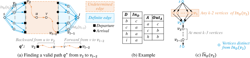
Figure 7. Illustrations for verifying undetermined edges

5.1. Departures and Arrivals

Besides departures $D$ and arrivals $A$, we further introduce the concept of Valid In-neighbors of Departures $In_{D}$ (resp. Valid Out-neighbors of Arrivals $Out_{A}$) that connect $s$ and departure (resp. arrival and $t$). As illustrated in Figure 7(a), $v_{2}$ is a departure vertex and $v_{l-2}$ is an arrival vertex, and $v_{1}\in In_{D}(v_{2})$ ($v_{l-1}\in Out_{A}(v_{l-2})$) since it connects $s$ and $v_{2}$ ($v_{l-2}$ and $t$).

Definition 5.1.

(Departure Vertex Set $D$). Vertex $v\in D$ iff there exists an in-neighbor $x$ of $v$ s.t. (1) $x$, $v$, $s$ and $t$ are distinct; and (2) edges $e(s,x)$ and $e(x,v)$ are contained in $SPG_{k}^{u}(s,t)$.

Definition 5.2.

(Valid In-neighbors of Departures, denoted as $In_{D}(v)$). For each $v\in D$, vertex $x\in In_{D}(v)$ iff it makes the two conditions in Definition 5.1 hold.

Definition 5.3.

(Arrival Vertex Set $A$). Vertex $v\in A$ iff there exists an out-neighbor $y$ of $v$ s.t. (1) $v$, $y$, $s$ and $t$ are distinct; (2) edges $e(v,y)$ and $e(y,t)$ are contained in $SPG_{k}^{u}(s,t)$.

Definition 5.4.

(Valid Out-neighbors of Arrivals $Out_{A}(v)$). For each $v\in A$, vertex $y\in Out_{A}(v)$ iff requirements (1) and (2) are satisfied in Definition 5.3.

By Lemmas 4.4 and 4.6, edges $e(s,x)$, $e(x,v)$ in Definition 5.1 and edges $e(v,y)$, $e(y,t)$ in Definition 5.3 are definite edges.

Example 5.5.

Consider the graph $G$ in Figure 6(c), when $k=7$, its departure vertex set $D$ and arrival vertex set $A$ are shown in Figure 7(b). For departure vertex $c$, its valid in-neighbor $In_{D}(c)=\{a\}$ since edges $e(s,a)$, $e(a,c)\in SPG_{k}^{u}(s,t)$. Meanwhile, $c$ is also an arrival and its valid out-neighbor $Out_{A}(c)=\{b\}$.

Departure vertex set $D$ and their valid in-neighbors $In_{D}$ can be collected with second-hop edges (as illustrated in Figure 6(e)). Notice that in Algorithm 2, when both $EV^{\ast}_{1}(s,u)$ and $EV_{k-1}^{\ast}(v,t)$ exist, and $u\notin EV_{k-2}^{\ast}(v,t)$, it labels edge $e(u,v)$ as a definite edge (line 5). When these constraints are met, $s$, $u$, $v$, and $t$ are distinct and $e(s,u)$ is contained in $SPG_{k}^{u}(s,t)$, which indicates that $v$ is a departure vertex and $u$ is a valid in-neighbor of $v$. Hence, to obtain departures $D$ and $In_{D}$, we only need to add such $v$ into $D$ and $u$ into $In_{D}(v)$ while labeling edges in line 5. Similarly, arrivals $A$ and $Out_{A}$ can also be collected.

Algorithm 3 Undetermined Edge Verification

1:Query variables ($s$, $t$, $k$), upper-bound graph $SPG_{k}^{u}$, departures $D$, arrivals $A$, valid in-neighbors $In_{D}$, and valid out-neighbors $Out_{A}$.

2:All edges in $SPG_{k}$.

3:$E(SPG_{k})\leftarrow$ All definite edges in $SPG_{k}^{u}$

4:if $k\geq 5$ then

5:    for each undetermined edge $e(u,v)\not\in E(SPG_{k})$ do

6:        $stk_{v}\leftarrow\{u,v,s,t\}$, $stk_{e}\leftarrow\{e(u,v)\}$

7:        Forward($v$, $1$, $u$)     

8:return $E(SPG_{k})$

9:function Forward($cur$, $l$, $u$)

10:    if $cur\in A$ $\land$ Backward($u$, $l$, $cur$) then return $True$     

11:    if $l<k-4$ then

12:        for each out-edge $e(cur,nxt)$ in $SPG_{k}^{u}$ s.t. $nxt\not\in stk_{v}$ do

13:           Push $nxt$ into $stk_{v}$, push $e(cur,nxt)$ into $stk_{e}$

14:           if Forward($nxt$, $l+1$, $u$) then return $True$            

15:           Pop $nxt$ from $stk_{v}$, pop $e(cur,nxt)$ from $stk_{e}$             

16:    return $False$

17:function Backward($cur$, $l$, $arrival$)

18:    if $cur\in D$ $\land$ TryAddEdges($cur$, $arrival$) then return $True$     

19:    if $l<k-4$ then

20:        for each in-edge $e(nxt,cur)$ in $SPG_{k}^{u}$ s.t. $nxt\not\in stk_{v}$ do

21:           Push $nxt$ into $stk_{v}$, push $e(nxt,cur)$ into $stk_{e}$

22:           if Backward($nxt$, $l+1$, $arrival$) then return $True$            

23:           Pop $nxt$ from $stk_{v}$, pop $e(nxt,cur)$ from $stk_{e}$             

24:    return $False$

25:function TryAddEdges($departure$, $arrival$)

26:    $In_{D}^{c}\leftarrow\{x\mid x\in In_{D}(departure)\land x\not\in stk_{v}\}$

27:    $Out_{A}^{c}\leftarrow\{y\mid y\in Out_{A}(arrival)\land y\not\in stk_{v}\}$

28:    if $\exists x\in In_{D}^{c},\;\exists y\in Out_{A}^{c}$ s.t. $x\neq y$ then

29:        $E(SPG_{k})\leftarrow E(SPG_{k})\cup stk_{e}$, return $True$     

30:    return $False$

5.2. DFS-oriented Search

As shown in Figure 7(a), for concluding that the undetermined edge $e(u,v)\in SPG_{k}$, intuitively we need to find a simple path $q^{\ast}$ from departure $v_{2}$ to arrival $v_{l-2}$ through edge $e(u,v)$, s.t. joining $s$, $v_{1}$, $q^{\ast}$, $v_{l-1}$, and $t$ produces a desired $s$-$t$ simple path. We then formalize the requirements for $q^{\ast}$ into the following theorem.

Theorem 5.6.

Undetermined edge $e(u,v)\in SPG_{k}(s,t)\Leftrightarrow$ there exists a simple path $q^{\ast}=\{v_{2},v_{3},\ldots,$ $v_{l-2}\}$ through $e(u,v)$ within $k-4$ hops, where (1) $v_{2}\in D$ $\land$ $v_{l-2}\in A$; and (2) $\exists v_{1}\in In_{D}(v_{2})$, $\exists v_{l-1}\in Out_{A}(v_{l-2})$ s.t. vertices $s,v_{1},v_{2},\ldots,$ $v_{l-1},t$ are distinct.

Proof.

Undetermined edge $e(u,v)$ is contained in $SPG_{k}(s,t)$ iff there exists an $s$-$t$ simple path $p^{\ast}=\{s=v_{0},v_{1},\ldots,v_{l-1},v_{l}=t\}$ through $e(u,v)$ s.t. $|p^{\ast}|=l\leq k$. Note that $e(u,v)$ is not in the first or last two steps of $p^{\ast}$, or it will not be an undetermined edge.

Necessity. Joining $e(s,v_{1})$, $e(v_{1},v_{2})$, edges in $q^{\ast}$, $e(v_{l-2},v_{l-1})$ and $e(v_{l-1},t)$ in order forms such a simple path $p^{\ast}$.

Sufficiency. $q^{\ast}$ can be extracted from $p^{\ast}$, which starts from $v_{2}$ and ends at $v_{l-2}$ with length $l-4\leq k-4$. By definitions, $v_{2}\in D$, $v_{l-2}\in A$, $v_{1}\in In_{D}(v_{2})$ and $v_{1-1}\in Out_{A}(v_{l-2})$. And vertices $s,v_{1},v_{2},\ldots,v_{l-1},t$ are distinct since they are in simple path $p^{\ast}$. ∎

Based on Theorem 5.6, we present Algorithm 3 to efficiently conclude whether an undetermined edge $e(u,v)$ is contained in $SPG_{k}(s,t)$. First, $E(SPG_{k})$ is initialized with all definite edges in line 3. In lines 4-7, for each undetermined edge $e(u,v)$, DFS-oriented search is conducted to find a valid path $q^{\ast}$ described in Theorem 5.6. As illustrated in Figure 7(a), it first tries to find a path from $v$ to an arrival $v_{l-2}$ (function Forward) and a path from a departure $v_{2}$ to $u$ (function Backward). The two paths are joined with $e(u,v)$, forming a path $q^{\ast}$ from departure $v_{2}$ to arrival $v_{l-2}$. If $q^{\ast}$ passes verification in function TryAddEdges, edges in $q^{\ast}$ will be added into $E(SPG_{k})$. Let us consider the following example.

Example 5.7.

For graph $G$ in Figure 6(c) with $k=7$, to verify the undetermined edge $e(i,j)$, we search forward from vertex $j$ and visit edge $e(j,h)\in SPG_{k}^{u}$. Since an arrival vertex $h$ (see Figure 7(b)) is reached, we search backward from $i$ and find that $i$ is a departure vertex. DFS-oriented search terminates with a simple path $q^{\ast}=\{i,j,h\}$. According to Figure 7(b), since $In_{D}(i)=\{a\}$ and $Out_{A}(h)=\{b\}$ have distinct vertices from $q^{\ast}$ and $|q^{\ast}|\leq k-4$, all undetermined edges involved ($e(i,j)$ and $e(j,h)$) will be added to result set.

By Theorem 5.8, for any departure vertex $v\in D$ we only need to store at most $k-2$ vertices in $In_{D}(v)$, i.e., replacing $In_{D}(v)$ with $\widehat{In}_{D}(v)$, where $|In_{D}(v)|$ denotes the size of $In_{D}(v)$ and

$$\widehat{In}_{D}(v)=\left\{\begin{array}[]{ll}\text{any $k-2$ vertices in $In_{D}(v)$},&|In_{D}(v)|>k-2;\\ In_{D}(v),&\text{otherwise}.\end{array}\right.$$

Theorem 5.8.

Theorem 5.6 holds if replacing $In_{D}$ with $\widehat{In}_{D}$.

Proof.

We just need to consider the case that $|In_{D}(v_{2})|>k-2$. Recall that $In_{D}(v)$ is involved only in requirement (2) of Theorem 5.6, which is $\exists v_{1}\in In_{D}(v_{2})$, $\exists v_{1-1}\in Out_{A}(v_{l-2})$ s.t. vertices $s,t,v_{1},v_{2},\ldots,v_{l-1}$ are distinct ($l\leq k$). Without loss of generality, assume that vertices $s,t,v_{2},v_{3},\ldots,v_{l-1}$ are fixed and already distinct, as illustrated in Figure 7(c). We need to prove that given $|In_{D}(v_{2})|>k-2$, $\exists v_{1}\in In_{D}(v_{2})$ s.t. $v_{1}$ is distinct from $s,t,v_{2},v_{3},\ldots,v_{l-1}$ iff $\exists v_{1}\in\widehat{In}_{D}(v_{2})$ s.t. $v_{1}$ is distinct from $s,t,v_{2},v_{3},\ldots,v_{l-1}$.

By Definition 5.2, $\forall x\in\widehat{In}_{D}(v_{2})\subseteq In_{D}(v_{2})$, $x$ is distinct from $s$, $t$ and $v_{2}$. To prove sufficiency, notice that number of the other vertices $v_{3},v_{4},\ldots,v_{l-1}$ is $l-3\leq k-3$, and we have $k-2$ vertices in $\widehat{In}_{D}(v_{2})$. Hence, $\exists v_{1}\in\widehat{In}_{D}(v_{2})$ s.t. $v_{1}$ is distinct from $s,t,v_{2},v_{3},\ldots,v_{l-1}$. Necessity is trivial since $\widehat{In}_{D}(v_{2})\subseteq In_{D}(v_{2})$. ∎

Similarly, at most $k-2$ vertices of $Out_{A}(v)$ will be materialized for any arrival vertex $v\in A$.

Time complexity of Verification. Recall that $D$, $A$, $In_{D}$ and $Out_{A}$ can be collected within $\mathcal{O}(|E|)$ time. For each undetermined edge $e(u,v)$, DFS-oriented search tries to find a simple path $q^{\ast}$ through $e(u,v)$ within $k-4$ hops, which takes $\mathcal{O}(d_{max}^{k-5})$ time and $d_{max}$ is the largest in-degree or out-degree of vertices in $SPG_{k}^{u}$. Further verification in function TryAddEdges for each $q^{\ast}$ takes $\mathcal{O}(k)$, since at most $k-2$ vertices are stored in $\widehat{In}_{D}(v_{2})$ ($\widehat{Out}_{A}(v_{l-2})$) after replacing $In_{D}(v_{2})$ ($Out_{A}(v_{l-2})$). Therefore, verifying undetermined edges takes $\mathcal{O}(k|E|d_{max}^{k-5})$ in the worst.

Space complexity of Verification. The number of departures and arrivals are bounded by $\mathcal{O}(|V|)$, and for each departure (arrival) $v$, $|\widehat{In}_{D}(v)|\leq k-2$ ($\widehat{Out}_{A}(v)\leq k-2$). Stacks for vertices and edges have size $\mathcal{O}(k)$. Hence, the total space cost is $\mathcal{O}(k|V|)$.

Theorem 5.9.

For $k\leq 5$, EVE takes $\mathcal{O}(|E|)$ time and space.

Proof.

As discussed in Section 3, computing essential vertices takes $\mathcal{O}(k^{2}|E|)$ time and $\mathcal{O}(k^{2}|V|)$ space. In Section 4, labeling edges and generating upper-bound graph consume $\mathcal{O}(k^{2}|E|)$ time and $\mathcal{O}(|E|)$ space, while edge verification takes $\mathcal{O}(k|E|)$ time and $\mathcal{O}(k|V|)$ space when $k=5$. Therefore, both time and space complexity are $\mathcal{O}(|E|)$ by considering $k$ as a small constant when $k\leq 5$. ∎

5.3. Search Ordering Strategies

As shown in Section 6.6, $SPG^{u}_{k}$ is a tight upper-bound of the desired simple path graph $SPG_{k}$, i.e., for each undetermined edge, a valid simple path $q^{\ast}$ discussed in Theorem 5.6 probably exists. To further speed up DFS-oriented search, it is better to find a valid $q^{\ast}$ earlier, stop the search and return $True$ directly. Note that when $k=5$ such techniques are unnecessary, since the initial length $l=k-4=1$ indicates that neither forward nor backward exploration is needed.

Recall requirements in Theorem 5.6. To verify edge $e(u,v)$, we need vertices $v_{2}\in D$, $v_{l-2}\in A$, $v_{1}\in In_{D}(v_{2})$ and $v_{l-1}\in Out_{A}(v_{l-2})$, while vertex distinctness and length constraint of $q^{\ast}$ are considered too. Intuitively, when starting a forward search from $v$, if vertices closer to any arrival are explored first, the desired path $q^{\ast}$ within length constraint is more likely to be obtained. Moreover, when there are several arrivals in the next step, visiting the one with larger $|Out_{A}(v_{l-2})|$ helps to increase the chance of satisfying vertex distinctness. Such intuitions drive us to sort out-neighbors of each vertex in $SPG_{k}^{u}$ before conducting a DFS-oriented search. We sort them in ascending order of distance to the closest arrival vertex, and those with distance $0$ (i.e., arrivals) are sorted by size of $Out_{A}$ in descending order. Similarly, we can sort in-neighbors of each vertex in $SPG_{k}^{u}$ in ascending order of distance from the closest departure vertex, and those with distance $0$ (i.e., departures) are sorted by size of $In_{D}$ in descending order.

Calculating the distance from departures to vertices $w$ in $SPG_{k}^{u}$ costs $\mathcal{O}(|E|)$ time and space, since we can create a virtual vertex $r$ connecting to all departures, after which BFS is conducted from $r$ for obtaining such distances. Sorting in-neighbors of all vertices takes $\mathcal{O}(\sum_{w\in V(SPG_{k}^{u})}d_{w}\log(d_{w}))=\mathcal{O}(|E|\log(d_{max}))$, where $d_{w}$ denotes the in-degree of vertex $w$ in $SPG_{k}^{u}$. Since the same costs also hold for sorting out-neighbors, pre-computation for adjusting search orders totally takes $\mathcal{O}(|E|\log(d_{max}))$ time and $\mathcal{O}(|E|)$ space.

6. Experiments

6.1. Experimental Setup

Datasets. As summarised in Table 2, we use 15 real networks from a variety of domains, such as social networks, web graphs and biological networks, in the experiments. These graphs are downloaded from NetworkRepository (Rossi and Ahmed, 2015), SNAP (Leskovec and Krevl, 2014) and Konect (Kunegis, 2013). The number of vertices and edges ranges from thousands to billions.

Table 2. Networks for Experiments

Name	Dataset	$\mathbf{|V|}$	$\mathbf{|E|}$	$\mathbf{d_{avg}}$	Type
ps	econ-psmigr3	3.1K	540K	172	Economic
ye	bio-grid-yeast	6K	314K	52	Biological
wn	bio-WormNet-v3	16K	763K	47	Biological
uk	web-uk-2005	130K	12M	91	Web
sf	web-Stanford	282K	13M	46	Web
bk	web-baidu-baike	416K	3.3M	8	Web
tw	twitter-social	465K	835K	2	Miscellaneous
bs	web-BerkStan	685K	7.6M	11	Web
gg	web-Google	876K	5.1M	6	Web
hm	bn-human-Jung2015	976K	146M	150	Biological
wt	wikiTalk	2.4M	5M	2	Miscellaneous
lj	soc-LiveJournal1	4.8M	68M	14	Social
dl	dbpedia-link	18M	137M	7	Miscellaneous
fr	soc-friendster	66M	1.8B	28	Social
hg	web-cc12-hostgraph	89M	2B	23	Web

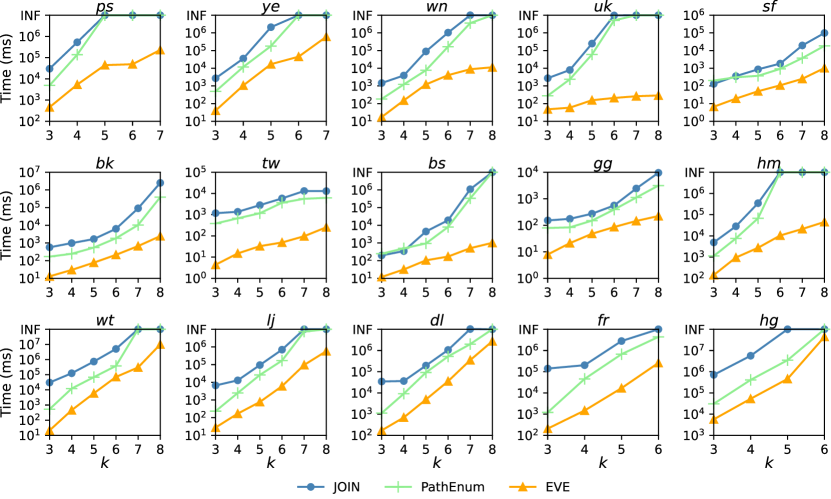
Figure 8. Total time cost of EVE and baselines

Queries. For each hop constraint $k$, we generate $1000$ random query pairs $(s,t)$ on each graph such that source vertex $s$ could reach target vertex $t$ in $k$ hops. Note that we focus on $k$-hop reachable query pairs, since the others can be efficiently filtered out by answering $k$-hop reachability queries (Cheng et al., 2012, 2014; Cai and Zheng, 2021). Similar to previous works of path enumeration (Peng et al., 2019, 2021; Sun et al., 2021), large $k$ is also not considered, since relation strength usually drops dramatically w.r.t $k$ and long paths are not useful to capturing the tie between vertices (Peng et al., 2021).

We conduct experiments on a Linux server with Intel(R) E5-2678v3 CPU @2.5GHz and 220G RAM. Programs are implemented in C++ and compiled with -O3 Optimization.

6.2. Performance Comparison with Baselines

To generate $k$-hop-constrained $s$-$t$ simple path graph $SPG_{k}(s,t)$, enumerating all hop-constrained $s$-$t$ simple paths then put all edges and vertices of these paths together is a straightforward solution. JOIN (Peng et al., 2019, 2021) and PathEnum (Sun et al., 2021) are state-of-the-arts for path enumeration, which significantly outperform other approaches and are thus considered as baseline algorithms for generating $SPG_{k}(s,t)$. Note that given vertices $s$, $t$ and hop constraint $k$, the edges of each path found by JOIN or PathEnum will be inserted into a set $E(SPG_{k}(s,t))$ which will be returned as the answer. Our proposed algorithm is denoted as EVE.

Results on time efficiency. Total time cost of answering $1000$ queries for each graph with different $k$ are shown in Figure 8, where the running time is set to INF if an algorithm does not terminate in $1\times 10^{7}$ ms ($1\times 10^{8}$ ms for graphs wt and hg). EVE is clear the most efficient on all graphs and $k$, and generally at least an order of magnitude faster than baselines. As expected, the time cost increases as $k$ grows for all algorithms. Moreover, the gap between EVE and the baselines gets larger on dense graphs, such as ps, ye, wn, uk and hm. It is because paths’ amount grows exponentially with large base of exponent, but edges’ amount is bounded by $|E|$, as illustrated in Figure 2(b). EVE even outperforms baselines by $4$ orders of magnitude on graph uk when $k\geq 6$. The scalability of EVE is also confirmed on billion-scale graphs fr and hg, while baselines may run out of time when $k=6$. For example, EVE only takes $0.26$s to answer each query on average over graph fr when $k=6$.

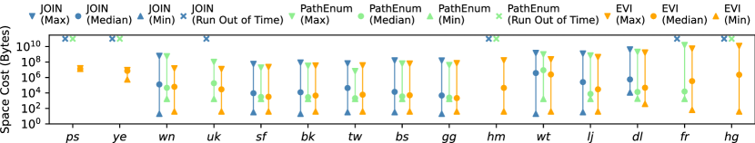
Figure 9. Maximum, median, and minimum space cost among 1000 queries ($k=6$)

Results on space cost. Since space consumption varies for different queries, we report the maximum, median, and minimum space cost among $1000$ queries for each graph when $k=6$ in Figure 9. We then focus on maximum space cost since an algorithm needs large enough memory for certain queries. JOIN demands the largest space cost since partial paths are stored before joining to obtain an $s$-$t$ path. PathEnum takes less space since its pre-built index helps to reduce the number of partial paths when the join-based method is adopted. On graphs sf, bk, tw and gg, EVE requires larger space compared with PathEnum. It is because these graphs have fewer desired paths, indicating that less space is needed to store partial paths for PathEnum, while $\mathcal{O}(k^{2}|V|)$ space is consumed to store essential vertices for EVE. We further investigate how $k$ influences the maximum space cost by taking graphs wn and bs as examples, as shown in Figure 10(a). As $k$ increases, baselines take much larger space, since the number of paths grows exponentially and storing partial paths is space inefficient. For EVE, we notice that space cost grows rapidly from $k=4$ to $k=5$, since undetermined edges, departures, arrivals and their neighbors are maintained for verification when $k\geq 5$.

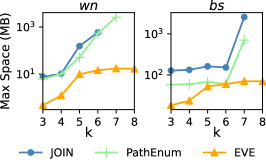
(a) Maximum space cost for graphs wn and bs

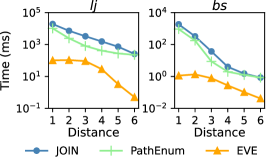
(b) Average query time for varying distances between query vertices $s$ and $t$ on graphs lj and bs ($k=6$)

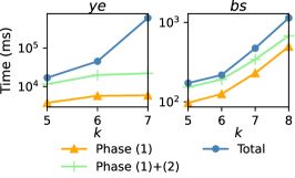
(c) Detailed time cost for graphs ye and bs

Figure 10. Maximum space cost, average query time for varying distances, and detailed time cost

6.3. Effect of Distances Between Query Pairs

For different shortest distances $\Delta(s,t)$ of query pairs ($s,t$), EVE is robust and significantly outperforms baselines. Take graphs $lj$ and $bs$ as examples, when $k=6$ we generate 500 random queries for each distance $1,2,\cdots,6$. As reported in Figure 10(b), when $\Delta(s,t)$ is closer to $k$, the number of paths is likely to decrease, and less time is required for all algorithms. EVE always has much shorter running time, especially for small distances. Intuitively, if $s$ and $t$ are closely connected, they tend to have more paths within $k$ hops.

6.4. Detailed Time Cost of EVE method

We further investigate the detailed time cost of three phases in EVE, i.e., (1) propagation for essential vertices, (2) computing upper-bound graph and (3) verifying undetermined edges. Taking dense graph ye and sparse graph bs as examples, their detailed time cost for $k\geq 5$ is shown in Figure 10(c). As $k$ increases, the time cost for phase (3) grows rapidly in graph ye due to its dense structure. For graph bs, the first two phases dominate the total cost, i.e., the cost of verifying undetermined edges is marginal compared with the cost of generating the upper-bound graph.

Table 3. Average redundant ratio $r_{D}$

$k$	ps	ye	wn	uk	st	bk	tw	bs
$5$	0.000004%	0.02%	$0$	$0$	0.49%	0.01%	$0$	0.31%
$6$	$0$	0.009%	$0$	$0$	0.84%	0.03%	$0$	0.45%
$7$	$0$	0.002%	$0$	$0$	1.4%	0.001%	0.004%	0.74%
$8$	-	-	$0$	$0$	1.6%	0.02%	0.01%	0.95%
$k$	gg	hm	wt	lj	dl	fr	hg
$5$	0.09%	$0$	0.00006%	$0$	$0$	$0$	$0$
$6$	0.12%	$0$	0.001%	0.0002%	0.0003%	$0$	0.002%
$7$	0.19%	$0$	0.002%	0.001%	0.0009%	-	-
$8$	0.13%	$0$	0.002%	0.004%	0.003%	-	-

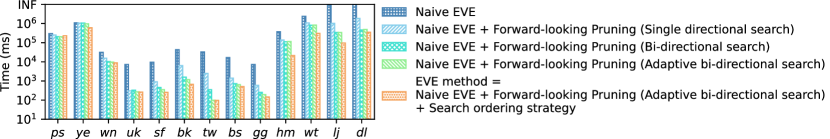
Figure 11. Effectiveness of pruning strategies for EVE ($k=7$)

6.5. Effectiveness of Pruning Strategies

We evaluate the effectiveness of our proposed pruning techniques including forward-looking pruning strategy (Section 3.3) and search ordering strategy (Section 5.3). Figure 11 reports the time cost of different versions that are equipped with distinct pruning techniques, where $k$ is set to $7$ by default and Naive EVE is the one disabling all pruning techniques above. With forward-looking pruning, running time on all graphs can be reduced up to an order of magnitude. The adaptive bi-directional search is faster than both single and bi-directional search. The search ordering strategy works effectively on most graphs except ps, since the re-ordering cost is not paid off. Note that ps has the largest average degree $172$, and finding a valid path is much easier in such a dense graph.

6.6. Coverage Ratio and Redundant Ratio

Evaluating the coverage ratio. Since the number of edges in $SPG_{k}$ (denoted by $|E(SPG_{k})|$) are bounded by $|E|$, we define the coverage ratio as $r_{C}=\frac{|E(SPG_{k})|}{|E|}$ ($r_{C}\leq 1$). Figure 12(a) presents the average coverage ratio with respect to different $k$ among all graphs. To make it clear, we split the results into two subfigures. We can see that graphs with larger average vertex degree tend to have higher coverage ratios, since larger degree indicates denser connection between query vertices $s$ and $t$ intuitively.

Evaluating the redundant ratio. We compare the size of upper-bound graph $SPG_{k}^{u}$ with the answer graph $SPG_{k}$ for $k\geq 5$, since $SPG_{k}^{u}=SPG_{k}$ when $k\leq 4$. To measure the difference between the number of edges in $SPG_{k}^{u}$ and $SPG_{k}$, we define redundant ratio as $r_{D}=\frac{|E(SPG_{k}^{u})|-|E(SPG_{k})|}{|E(SPG_{k})|}$ for each query. Average $r_{D}$ for queries on each graph and $k$ are summarised in Table 3, where $0$ indicates that $SPG_{k}^{u}=SPG_{k}$. For most graphs except graphs st, bs and gg, $SPG_{k}^{u}$ only has less than $0.05\%$ redundant edges. Hence, $SPG_{k}^{u}$ computed in $\mathcal{O}(k^{2}|E|)$ is quite tight, reducing the search space sharply.

Table 4. Speedups for hop-constrained s-t path enumeration

	$k$	ps	sf	bk	tw	bs	wt	lj	dl	fr	hg
KHSQ	3	0.4	0.4	0.2	0.2	0.3	<0.1	<0.1	<0.1	<0.1	¡0.1
	4	0.8	0.2	0.1	0.1	0.2	0.1	<0.1	<0.1	¡0.1	<0.1
	5	0.6	0.3	0.1	0.2	0.2	0.6	<0.1	<0.1	¡0.1	¡0.1
	6	-	0.2	0.1	0.5	0.3	0.5	<0.1	0.1	¡0.1	-
KHSQ+	3	0.7	1.6	1.5	3.7	1.3	0.3	0.2	0.1	0.2	0.2
	4	0.8	0.9	1.1	3.1	1.1	2.2	0.4	0.5	1.0	0.5
	5	0.6	2.1	1.9	11.8	1.2	1.4	2.5	1.6	3.2	1.2
	6	-	1.5	1.9	23	0.7	0.8	3.6	2.3	1.7	-
EVE	3	3.1	1.4	2.6	2.2	2.2	4.3	1.2	2.0	3.1	4.0
	4	1.3	1.9	2.1	3.4	1.8	15.2	4.1	7.4	23.1	6.6
	5	1.0	4.3	4.8	16.1	2.2	9.5	22.4	13.0	36.7	6.1
	6	-	1.9	3.5	38.5	1.1	1.4	20.0	10.7	12	-

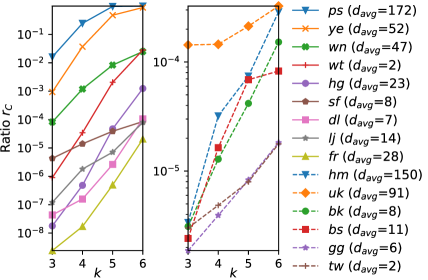
(a) Average coverage ratio $r_{C}$ vs. $k$

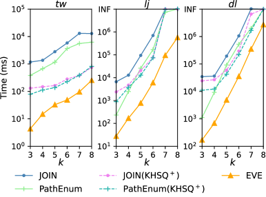
(b) Compare with baselines on graphs tw, lj, and dl

Figure 12. Effect of $k$ on the average coverage ratio and time efficiency.

6.7. Speedups for Simple Path Enumeration

We conduct experiments to illustrate that the simple path graph $SPG_{k}(s,t)$ helps to speed up hop-constrained $s$-$t$ path enumeration. PathEnum (Sun et al., 2021) is the state-of-art algorithm for path enumeration. For each query $\langle s,t,k\rangle$, we can first compute $SPG_{k}(s,t)$ by our proposed method EVE and then use it as search space for PathEnum, i.e., replacing the original graph $G$ with $SPG_{k}(s,t)$.

Speedups ($\frac{\text{time of {PathEnum} on the original graph }G}{\text{time of {PathEnum} on }SPG_{k}(s,t)+\text{time of generating }SPG_{k}(s,t)}$) by varying datasets and $k$ are summarised in Table 4. For graphs tw, wt, lj, dl, and fr, PathEnum can be accelerated by up to an order of magnitude without any modification.

Moreover, the $k$-hop $s$-$t$ subgraph $G_{st}^{k}$ (Liu et al., 2021) can also be used as search space for PathEnum, which contains all $s$-$t$ paths within $k$ hops but those paths are not required to be simple paths. However, generating $G_{st}^{k}$ with the state-of-the-art KHSQ algorithm (Liu et al., 2021) cannot accelerate PathEnum (speedups $<1$), as shown in Table 4. And we further develop its optimized algorithm KHSQ⁺, using adaptive bi-directional search (see Section 3.3) instead of single directional BFS in KHSQ for distance computation. KHSQ⁺ has much better performance than KHSQ, but is still less efficient than $SPG_{k}(s,t)$ that is generated by EVE, since $SPG_{k}(s,t)$ is a subgraph of $G_{st}^{k}$ and some time-consuming cycles contained in $G_{st}^{k}$ are avoided for PathEnum.

6.8. Generating Simple Path Graph based on $\mathbf{G_{st}^{k}}$

For generating $SPG_{k}(s,t)$, we can first compute $G_{st}^{k}$ and then apply JOIN (Peng et al., 2019, 2021) (PathEnum (Sun et al., 2021)) on $G_{st}^{k}$. As discussed in Section 6.7, KHSQ⁺ is used instead of KHSQ (Liu et al., 2021) for efficiently computing $G_{st}^{k}$. In this way, the modified JOIN (PathEnum) for generating $SPG_{k}(s,t)$ is faster than naive baselines. Table 5 reports speedups ($\frac{\text{Time cost of {JOIN} ({PathEnum}) on }G}{\text{Time cost of {JOIN} ({PathEnum}) on }G_{st}^{k}}$) for $k=6$ except those run out of time. However, by varying $k$ they are still not comparable with the proposed EVE method. As shown in Figure 12(b), even for graphs tw, lj, and dl where significant speedups are achieved in Table 5, EVE is still far more efficient than baselines enhanced by KHSQ⁺.

Table 5. Speedups for generating $\mathbf{SPG_{k}(s,t)}$ on $\mathbf{G^{k}_{st}}$ ($\mathbf{k=6}$)

Dataset	wn	uk	sf	bk	tw	bs	gg	wt	lj	dl	fr
JOIN	$1.3$	$2.1$	$1.4$	$1.9$	$20.7$	$0.4$	$0.8$	$3.1$	$9.2$	$3.6$	-
PathEnum	$0.9$	$2.5$	$1.9$	$1.3$	$16.0$	$0.5$	$1.1$	$0.9$	$2.3$	$2.4$	$2.6$

6.9. Case Study

It has been shown that simple path graph works for visualizing connections between vertices $s$ and $t$ in Figure 2. Next, we introduce how EVE helps identify fraudulent activities in a transaction network with millions of vertices and edges from an e-commerce company. For a transaction (edge) $e(t,s)$ at time $T_{0}$, the goal is to find vertices and edges involved in any $(k+1)$-hop constrained cycles through $e(t,s)$, where all transaction time is required to be within $\Delta T$ days (i.e., only consider edges at time $[T_{0}-\Delta T,T_{0}]$ when searching). The generated $SPG_{k}(s,t)$ for $k=5$ and $\Delta T=7$ is shown in Figure 13(a), in which accounts (vertices) and transactions (edges) are suspicious since they form simple cycle(s) in a short time period.

7. Related Work

In this section, we review related $s$-$t$ queries which are widely applied in the real world, as summarized in Figure 13(b).

Reachability and $k$-hop reachability Query. Answering reachability queries is one of the fundamental graph queries and has been extensively studied (Su et al., 2017; Yano et al., 2013; Cheng et al., 2013; Wei et al., 2018; Yildirim et al., 2012; Veloso et al., 2014; Zhou et al., 2018). Since the number of hops indicates the level of influence $s$ has over $t$, many applications can benefit from $k$-hop reachability queries, which asks whether a vertex $s$ can reach $t$ within $k$ hops (Cheng et al., 2012, 2014; Xie et al., 2017; Du et al., 2019; Cai and Zheng, 2021). $k$-hop reachability problem is more general since when $k=\infty$, we can obtain the answer to the reachability problem.

Path Graph Queries. QbS (Wang et al., 2021) defines an $s$-$t$ shortest path graph (Wang et al., 2021) that contains exactly all the shortest paths from $s$ to $t$. It computes a sketch from the labeling scheme and then conducts an online search to return the exact answer. However, the information provided by shortest path graph may be too limited, since paths slightly longer than shortest distance may also be of user interest. It is not trivial to extend QbS to our problem, since it is still inevitable for examining edges out of shortest path graph when $k$ is larger than shortest distance. Liu et al. (Liu et al., 2021) defines the $k$-hop $s$-$t$ subgraph query which returns the subgraph containing all paths from $s$ to $t$ within $k$ hops, but those paths are not required to be simple paths. TransferPattern (Bast et al., 2010) delivers a graph that just contains multi-criteria shortest paths by allowing multiple copies of vertices. It not only increases the size but also is unfriendly to display the underlying connections as it is not a subgraph of the input graph.

(Hop-constrained) Simple Path Enumeration. There have been a bunch of works for simple path enumeration (Grossi, 2016; Yang et al., 2015; Birmelé et al., 2013; Grossi et al., 2018). Hop-constrained $s$-$t$ simple path enumeration aims at finding all simple paths from $s$ to $t$ within $k$ hops, and recent works include TDFS (Rizzi et al., 2014), BC-DFS, JOIN (Peng et al., 2019, 2021) and PathEnum (Sun et al., 2021). TDFS (Rizzi et al., 2014) ensures that each vertex $v$ explored during forward DFS will produce at least an output path, which is achieved by backward BFS from target vertex $t$ at each step. BC-DFS (Peng et al., 2019, 2021) is a barrier-pruning-based DFS algorithm, which prevents falling into the same trap twice by maintaining barriers during exploration. To improve query response time, JOIN (Peng et al., 2019, 2021) first finds some cutting vertices, then concatenates partial paths enumerated by BC-DFS. The time complexity of TDFS, BC-DFS and JOIN are $\mathcal{O}(\delta k|E|)$, where $\delta$ is the number of output paths. PathEnum (Sun et al., 2021) first builds a lightweight online index based on shortest distances, then uses a cost-based query optimizer to select DFS-based or join-based method for answering queries. As discussed before, enumerating all $k$-hop-constrained $s$-$t$ simple paths by above approaches is a straightforward solution for generating simple path graph $SPG_{k}(s,t)$. On the other hand, with the output $SPG_{k}(s,t)$ from our EVE method, these approaches can also be accelerated by taking $SPG_{k}(s,t)$ as their search space.

Pruning Techniques. Forward-looking pruning adopts the general idea of checking distances (Rizzi et al., 2014; Liu et al., 2021). In (Rizzi et al., 2014) distances are computed at each step of DFS, since vertices in DFS stack are removed to avoid vertex reuse for simple path. In contrast, (Liu et al., 2021) pre-computes all distances once but paths are not required to be simple. EVE targets at the simple path graph, but also computes distances only once since essential vertices encode vertex reuse. Moreover, though the idea of vertex reordering has been widely used with various goals (Wang et al., 2021; Yano et al., 2013; Ueno et al., 2017; Ahmadi et al., 2021; Peng et al., 2020), search ordering strategies are developed based on the tight upper-bound graph and use specialized keys (distance, $|In_{D}|$ and $|Out_{A}|$) for sorting neighbors to find valid paths earlier.

To prune spurious candidates when addressing the subgraph isomorphism problem, the algorithm KARPET (Tziavelis et al., 2020; Yang et al., 2018) adopts the idea of two-phase traversal similar to bi-directional propagation, but utilizes the query pattern to remove the vertices against the label constraints from the candidate graph in the first traversal.

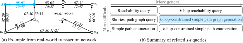
Figure 13. Case study and summary of related work

8. Conclusion

In this paper, we formalize the $k$-hop-constrained $s$-$t$ simple path graph generation problem, which has a wide range of applications. We prove its NP-hardness on directed graphs and propose a method EVE to tackle this challenging problem. It does not need to enumerate all paths powered by the essential vertices. Moreover, a tight upper-bound graph is derived. To verify undetermined edges, a DFS-oriented search based on carefully designed orders is proposed. Extensive experiments show that EVE significantly outperforms all baselines, and it also helps to accelerate other graph queries such as hop-constrained simple path enumeration.

- (1)
- Ahmadi et al. (2021) Saman Ahmadi, Guido Tack, Daniel Damir Harabor, and P. Kilby. 2021. A Fast Exact Algorithm for the Resource Constrained Shortest Path Problem. In AAAI.
- Ahuja et al. (1993) Ravindra K. Ahuja, Thomas L. Magnanti, and James B. Orlin. 1993. Network Flows: Theory, Algorithms, and Applications.
- Alon et al. (1995) Noga Alon, Raphael Yuster, and Uri Zwick. 1995. Color-coding. Journal of the ACM (JACM) 42, 4 (1995), 844–856.
- Baier et al. (2010) Georg Baier, Thomas Erlebach, Alexander Hall, Ekkehard Köhler, Petr Kolman, Ondrej Pangrác, Heiko Schilling, and Martin Skutella. 2010. Length-bounded cuts and flows. ACM Trans. Algorithms 7, 1 (2010), 4:1–4:27.
- Bast et al. (2010) Hannah Bast, Erik Carlsson, Arno Eigenwillig, Robert Geisberger, Chris Harrelson, Veselin Raychev, and Fabien Viger. 2010. Fast Routing in Very Large Public Transportation Networks Using Transfer Patterns. In Algorithms – ESA 2010. 290–301.
- Bäumer et al. (2014) Frederik Simon Bäumer, Jangwon Gim, Do-Heon Jeong, Michaela Geierhos, and Hanmin Jung. 2014. Linked Open Data System for Scientific Data Sets. In IPaMin 2014 (CEUR Workshop Proceedings, Vol. 1292).
- Birmelé et al. (2013) Etienne Birmelé, Rui A. Ferreira, Roberto Grossi, Andrea Marino, Nadia Pisanti, Romeo Rizzi, and Gustavo Sacomoto. 2013. Optimal Listing of Cycles and st-Paths in Undirected Graphs. In SODA 2013. 1884–1896.
- Cabrera et al. (2020) Nicolás Cabrera, Andrés L. Medaglia, Leonardo Lozano, and Daniel Duque. 2020. An exact bidirectional pulse algorithm for the constrained shortest path. Networks 76, 2 (2020), 128–146.
- Cai and Zheng (2021) Yuzheng Cai and Weiguo Zheng. 2021. ESTI: Efficient k-Hop Reachability Querying over Large General Directed Graphs. In DASFAA 2021 International Workshops - BDQM, GDMA, MLDLDSA, MobiSocial, and MUST. Springer, 71–89.
- Cheng et al. (2013) James Cheng, Silu Huang, Huanhuan Wu, and Ada Wai-Chee Fu. 2013. TF-Label: a topological-folding labeling scheme for reachability querying in a large graph. In SIGMOD 2013. 193–204.
- Cheng et al. (2012) James Cheng, Zechao Shang, Hong Cheng, Haixun Wang, and Jeffrey Xu Yu. 2012. K-Reach: Who is in Your Small World. Proc. VLDB Endow. 5, 11 (2012), 1292–1303.
- Cheng et al. (2014) James Cheng, Zechao Shang, Hong Cheng, Haixun Wang, and Jeffrey Xu Yu. 2014. Efficient processing of k-hop reachability queries. VLDB J. 23, 2 (2014), 227–252.
- Du et al. (2019) Ming Du, Anping Yang, Junfeng Zhou, Xian Tang, Ziyang Chen, and Yanfei Zuo. 2019. HT: A Novel Labeling Scheme for k-Hop Reachability Queries on DAGs. IEEE Access 7 (2019), 172110–172122.
- Fomin et al. (2018) Fedor V Fomin, Daniel Lokshtanov, Fahad Panolan, Saket Saurabh, and Meirav Zehavi. 2018. Long directed (s, t)-path: FPT algorithm. Inform. Process. Lett. 140 (2018), 8–12.
- Fortune et al. (1980) Steven Fortune, John E. Hopcroft, and James Wyllie. 1980. The Directed Subgraph Homeomorphism Problem. Theor. Comput. Sci. 10 (1980), 111–121.
- García-Godoy et al. (2011) María Jesús García-Godoy, Ismael Navas Delgado, and José Francisco Aldana Montes. 2011. Bioqueries: a social community sharing experiences while querying biological linked data. In SWAT4LS 2011. 24–31.
- Goldberg and Harrelson (2005) Andrew V. Goldberg and Chris Harrelson. 2005. Computing the shortest path: A search meets graph theory. symposium on discrete algorithms (2005).
- Grossi (2016) Roberto Grossi. 2016. Enumeration of Paths, Cycles, and Spanning Trees. In Encyclopedia of Algorithms. 640–645.
- Grossi et al. (2018) Roberto Grossi, Andrea Marino, and Luca Versari. 2018. Efficient Algorithms for Listing k Disjoint st-Paths in Graphs. In LATIN 2018, Vol. 10807. 544–557.
- Heim et al. (2009) Philipp Heim, Sebastian Hellmann, Jens Lehmann, Steffen Lohmann, and Timo Stegemann. 2009. RelFinder: Revealing Relationships in RDF Knowledge Bases. In SAMT 2009, Vol. 5887. 182–187.
- Holzer et al. (2005) Martin Holzer, Frank Schulz, Dorothea Wagner, and Thomas Willhalm. 2005. Combining speed-up techniques for shortest-path computations. ACM Journal of Experimental Algorithms (2005).
- Kunegis (2013) Jérôme Kunegis. 2013. KONECT: the Koblenz network collection. In WWW ’13. 1343–1350.
- Leskovec et al. (2010) Jure Leskovec, Daniel Huttenlocher, and Jon Kleinberg. 2010. Signed networks in social media. In Proceedings of the SIGCHI conference on human factors in computing systems. 1361–1370.
- Leskovec and Krevl (2014) Jure Leskovec and Andrej Krevl. 2014. SNAP Datasets: Stanford Large Network Dataset Collection.
- Liu et al. (2021) Yu Liu, Qian Ge, Yue Pang, and Lei Zou. 2021. Hop-Constrained Subgraph Query and Summarization on Large Graphs. In DASFAA 2021 International Workshops - BDQM, GDMA, MLDLDSA, MobiSocial, and MUST, Vol. 12680. 123–139.
- Lohmann et al. (2010) Steffen Lohmann, Philipp Heim, Timo Stegemann, and Jürgen Ziegler. 2010. The RelFinder user interface: interactive exploration of relationships between objects of interest. In IUI 2010. 421–422.
- Peng et al. (2021) You Peng, Xuemin Lin, Ying Zhang, Wenjie Zhang, Lu Qin, and Jingren Zhou. 2021. Efficient Hop-constrained s-t Simple Path Enumeration. VLDB J. 30, 5 (2021), 799–823.
- Peng et al. (2020) You Peng, Ying Zhang, Xuemin Lin, Lu Qin, and Wenjie Zhang. 2020. Answering Billion-Scale Label-Constrained Reachability Queries within Microsecond. Proc. VLDB Endow. 13, 6 (2020), 812–825.
- Peng et al. (2019) You Peng, Ying Zhang, Xuemin Lin, Wenjie Zhang, Lu Qin, and Jingren Zhou. 2019. Hop-constrained s-t Simple Path Enumeration: Towards Bridging Theory and Practice. Proc. VLDB Endow. 13, 4 (2019), 463–476.
- Qiu et al. (2018) Xiafei Qiu, Wubin Cen, Zhengping Qian, You Peng, Ying Zhang, Xuemin Lin, and Jingren Zhou. 2018. Real-time Constrained Cycle Detection in Large Dynamic Graphs. Proc. VLDB Endow. 11, 12 (2018), 1876–1888.
- Rizzi et al. (2014) Romeo Rizzi, Gustavo Sacomoto, and Marie-France Sagot. 2014. Efficiently Listing Bounded Length st-Paths. In IWOCA 2014, Vol. 8986. 318–329.
- Rossi and Ahmed (2015) Ryan A. Rossi and Nesreen K. Ahmed. 2015. The Network Data Repository with Interactive Graph Analytics and Visualization. In AAAI 2015. 4292–4293.
- Sobrinho and Ferreira (2020) João Luis Sobrinho and Miguel Alves Ferreira. 2020. Routing on Multiple Optimality Criteria. In SIGCOMM ’20. 211–225.
- Su et al. (2017) Jiao Su, Qing Zhu, Hao Wei, and Jeffrey Xu Yu. 2017. Reachability Querying: Can It Be Even Faster? TKDE 29, 3 (2017), 683–697.
- Sun et al. (2021) Shixuan Sun, Yuhang Chen, Bingsheng He, and Bryan Hooi. 2021. PathEnum: Towards Real-Time Hop-Constrained s-t Path Enumeration. In SIGMOD ’21. 1758–1770.
- Tziavelis et al. (2020) Nikolaos Tziavelis, Deepak Ajwani, Wolfgang Gatterbauer, Mirek Riedewald, and Xiaofeng Yang. 2020. Optimal Algorithms for Ranked Enumeration of Answers to Full Conjunctive Queries. Proc. VLDB Endow. 13, 9 (2020), 1582–1597.
- Ueno et al. (2017) Koji Ueno, Toyotaro Suzumura, Naoya Maruyama, Katsuki Fujisawa, and Satoshi Matsuoka. 2017. Efficient Breadth-First Search on Massively Parallel and Distributed-Memory Machines. Data Science and Engineering (2017).
- Veloso et al. (2014) Renê Rodrigues Veloso, Loïc Cerf, Wagner Meira Jr., and Mohammed J. Zaki. 2014. Reachability Queries in Very Large Graphs: A Fast Refined Online Search Approach. In EDBT 2014. 511–522.
- Wang et al. (2021) Ye Wang, Qing Wang, Henning Koehler, and Yu Lin. 2021. Query-by-Sketch: Scaling Shortest Path Graph Queries on Very Large Networks. In SIGMOD ’21. 1946–1958.
- Wang and Crowcroft (1996) Zheng Wang and Jon Crowcroft. 1996. Quality-of-Service Routing for Supporting Multimedia Applications. IEEE J. Sel. Areas Commun. 14, 7 (1996), 1228–1234.
- Wei et al. (2018) Hao Wei, Jeffrey Xu Yu, Can Lu, and Ruoming Jin. 2018. Reachability querying: an independent permutation labeling approach. VLDB J. 27, 1 (2018), 1–26.
- Xie et al. (2017) Xia Xie, Xiaodong Yang, Xiaokang Wang, Hai Jin, Duoqiang Wang, and Xijiang Ke. 2017. BFSI-B: An improved K-hop graph reachability queries for cyber-physical systems. Inf. Fusion 38 (2017), 35–42.
- Yang et al. (2015) Runtao Yang, Rui Gao, and Chengjin Zhang. 2015. A new algebraic approach to finding all simple paths and cycles in undirected graphs. In ICIA 2015. 1887–1892.
- Yang et al. (2018) Xiaofeng Yang, Deepak Ajwani, Wolfgang Gatterbauer, Patrick K. Nicholson, Mirek Riedewald, and Alessandra Sala. 2018. Any-k: Anytime Top-k Tree Pattern Retrieval in Labeled Graphs (WWW ’18). 489–498.
- Yano et al. (2013) Yosuke Yano, Takuya Akiba, Yoichi Iwata, and Yuichi Yoshida. 2013. Fast and scalable reachability queries on graphs by pruned labeling with landmarks and paths. In CIKM’13. 1601–1606.
- Yeh et al. (2012) Cheng-Yu Yeh, Hsiang-Yuan Yeh, Carlos Roberto Arias, and Von-Wun Soo. 2012. Pathway detection from protein interaction networks and gene expression data using color-coding methods and A* search algorithms. The Scientific World Journal 2012 (2012).
- Yildirim et al. (2012) Hilmi Yildirim, Vineet Chaoji, and Mohammed J. Zaki. 2012. GRAIL: a scalable index for reachability queries in very large graphs. VLDB J. 21, 4 (2012), 509–534.
- Zhou et al. (2018) Junfeng Zhou, Jeffrey Xu Yu, Na Li, Hao Wei, Ziyang Chen, and Xian Tang. 2018. Accelerating reachability query processing based on DAG reduction. VLDB J. 27, 2 (2018), 271–296.