CoDi: Co-evolving Contrastive Diffusion Models
for Mixed-type Tabular Synthesis

Abstract

With growing attention to tabular data these days, the attempt to apply a synthetic table to various tasks has been expanded toward various scenarios. Owing to the recent advances in generative modeling, fake data generated by tabular data synthesis models become sophisticated and realistic. However, there still exists a difficulty in modeling discrete variables (columns) of tabular data. In this work, we propose to process continuous and discrete variables separately (but being conditioned on each other) by two diffusion models. The two diffusion models are co-evolved during training by reading conditions from each other. In order to further bind the diffusion models, moreover, we introduce a contrastive learning method with a negative sampling method. In our experiments with 11 real-world tabular datasets and 8 baseline methods, we prove the efficacy of the proposed method, called CoDi. Our code is available at https://github.com/ChaejeongLee/CoDi.

1 Introduction

Tabular data is one of the most frequently occurring data types in real-world applications. Considering that tabular data attracts much attention these days (Borisov et al., 2021; Shwartz-Ziv & Armon, 2022; Yin et al., 2020; Gorishniy et al., 2021), synthesizing tabular data is a timely research issue. The quality of generated tabular data has significantly improved owing to recent advancements in the generative model paradigm (Park et al., 2018; Xu et al., 2019; Kim et al., 2021; Lee et al., 2021; Kim et al., 2022a).

In spite of the advancement, there still exists a challenging issue in the current state-of-the-art tabular data synthesis methods. To be specific, tabular data usually consists of mixed data types, i.e., continuous and discrete variables. Due to the complicated nature of tabular data, pre/post-processing of the tabular data is inevitable, and the performance of tabular data synthesis methods is highly dependent on the pre/post-processing method. While various processing methods for continuous variables have been proposed, e.g., standardizing continuous values using variational Gaussian mixture models (Xu et al., 2019) and applying the logarithm transformation to treat long-tailed distributions (Zhao et al., 2021), handling discrete variables remains challenging. The most common way to treat discrete variables is to sample in continuous spaces after their one-hot encoding (and sometimes via Gumbel-softmax) (Xu et al., 2019; Kim et al., 2021, 2022b, 2022a), which may lead to sub-optimal results due to sampling mistakes.

Moreover, treating discrete variables in continuous spaces is also problematic in terms of the entire learned data distribution. When continuous and discrete variables are processed in a same manner, it is likely that inter-column correlations — in particular, the correlation between continuous and discrete variables — are compromised in the learned distribution. Therefore, we are interested in processing continuous and discrete variables in more robust ways.

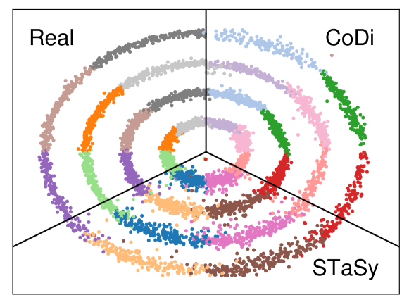
Figure 1: Preliminary experiment on a toy dataset. The dataset contains 4 columns, which are two continuous (the x-axis and y-axis) and two discrete (16 colors and 4 circles) columns. (Left) is a scatter plot of real data, (Bottom) is synthesized data by STaSy (Kim et al., 2022a), and (Right) is synthesized data by our proposed method. Detailed information and visualizations are in Appendix A.

In this paper, we propose a technique for tabular data synthesis that incorporates two diffusion models to handle continuous and discrete variables. To be specific, one diffusion model for continuous variables works in a continuous space, and the other works in a discrete space. For better learning the mixed data distribution, our proposed method contains two design points: i) co-evolving conditional diffusion models, and ii) contrastive training for better connecting them. In our description below, let $\mathbf{x}_{0}=(\mathbf{x}_{0}^{C},\mathbf{x}_{0}^{D})$, which consists of continuous and discrete values, be a sample (or record) of tabular data. $\mathbf{x}_{t}=(\mathbf{x}_{t}^{C},\mathbf{x}_{t}^{D})$ means its diffused sample at time (or step) $t$.

Co-evolving conditional diffusion models To make the two diffusion models able to synthesize one tabular data, we make them read conditions from each other as in Fig. 2. The two models simultaneously perturb continuous and discrete variables at each forward step. In detail, the continuous (resp. discrete) model reads the perturbed discrete (resp. continuous) sample as a condition at the same time step. For the reverse process of the continuous (resp. discrete) diffusion model, the model denoises the sample $\mathbf{x}_{t}^{C}$ (resp. $\mathbf{x}_{t}^{D}$) conditioned both on the continuous sample $\mathbf{x}_{t+1}^{C}$ and discrete sample $\mathbf{x}_{t+1}^{D}$ from its previous step.

Contrastive learning for tabular data To bind the two conditional diffusion models further, we design a contrastive learning method. Our contrastive learning process is applied to the continuous and discrete diffusion models separately. We also design a negative sampling method for tabular data, which focuses on defining a negative condition that permutes the pair of continuous and discrete variable sets. For simplicity but without loss of generality, we describe a process only for the continuous diffusion model (from which the contrastive learning for the discrete diffusion can be easily deduced). Given an anchor sample $\mathbf{x}_{0}^{C}$, we generate a continuous positive sample $\hat{\mathbf{x}}_{0}^{C+}$ from a continuous diffusion model conditioned on $\mathbf{x}_{0}^{D}$. For a negative sample $\hat{\mathbf{x}}_{0}^{C-}$, we randomly permute the condition parts, and therefore, negative condition $\mathbf{x}_{0}^{D-}$ is an inappropriate counterpart for $\mathbf{x}_{0}^{C}$. As a result, we generate $\hat{\mathbf{x}}_{0}^{C-}$ conditioned on $\mathbf{x}_{0}^{D-}$.

The two proposed design points for tabular data synthesis considerably improve the sampling quality over state-of-the-art methods. As shown in Fig. 1, our method demonstrates its overall efficacy, where Fig. 1 visualizes sampling outcomes with synthetic toy tabular data. In Sec. 4, we provide more details with our experiments on 11 datasets and 8 baselines showing that our method effectively models real-world tabular data distribution by processing mixed-type tabular data in the proper spaces.

We summarize the contributions of this paper as follows:

1. We propose to separately train two diffusion models for continuous and discrete variables which consist of tabular data, to better learn their own distributions. To our knowledge, we are the first proposing separately processing them with two physically separated models.

2. To bridge the two diffusion models, however, we propose to design them using co-evolving conditional continuous and discrete diffusion models, which are conditioned on each other. Moreover, we also design a contrastive learning method to reinforce the binding between the models further.

3. Consequently, the generative learning trilemma (Xiao et al., 2022), which is the 3 key requirements for generative models including the sampling quality, diversity, and sampling time, has been improved over state-of-the-art methods, as shown in Sec. 4.

2 Background

2.1 Diffusion Probabilistic Models

Diffusion probabilistic models (Sohl-Dickstein et al., 2015) are deep generative models defined from a forward and reverse Markov process. The forward process is to gradually corrupt a sample $\mathbf{x}_{0}$ into a noisy vector $\mathbf{x}_{T}$, as follows:

$$q(\mathbf{x}_{1:T}|\mathbf{x}_{0})\coloneqq\prod_{t=1}^{T}{q(\mathbf{x}_{t}|\mathbf{x}_{t-1})}.$$ (1)

The reverse process is to remove noises and generate a fake sample $\hat{\mathbf{x}}_{0}$ from $\mathbf{x}_{T}$, as follows:

$$p_{\theta}(\mathbf{x}_{0:T})\coloneqq p(\mathbf{x}_{T})\prod_{t=1}^{T}{p_{\theta}(\mathbf{x}_{t-1}|\mathbf{x}_{t})},$$ (2)

where $p_{\theta}(\mathbf{x}_{t-1}|\mathbf{x}_{t})$ represents the reverse of the forward transition probability, approximated by a neural network. The parameter $\theta$ optimizes a variational upper bound on the negative log-likelihood:

$$L_{\mathrm{vb}} =\mathbb{E}_{q}\bigg{[}\underbrace{D_{\mathrm{KL}}[q(\mathbf{x}_{T}|\mathbf{x}_{0})||p(\mathbf{x}_{T})]}_{L_{T}}\underbrace{-\log{p_{\theta}(\mathbf{x}_{0}|\mathbf{x}_{1})}}_{L_{0}}$$ (3)

$$+\sum_{t=2}^{T}\underbrace{{D_{\mathrm{KL}}(q(\mathbf{x}_{t-1}|\mathbf{x}_{t},\mathbf{x}_{0})||p_{\theta}(\mathbf{x}_{t-1}|\mathbf{x}_{t}))}}_{L_{t-1}}\bigg{]}.$$

2.1.1 Continuous Spaces

The diffusion process in continuous spaces (Ho et al., 2020) defines the forward and reverse transition probabilities with a prior distribution $p(\mathbf{x}_{T})=\mathcal{N}(\mathbf{x}_{T};\mathbf{0},\mathbf{I})$, as follows:

$$q(\mathbf{x}_{t}|\mathbf{x}_{t-1})=\mathcal{N}(\mathbf{x}_{t};\sqrt{1-\beta_{t}}\mathbf{x}_{t-1},\beta_{t}\mathbf{I}),$$ (4)

$$p_{\theta}(\mathbf{x}_{t-1}|\mathbf{x}_{t})=\mathcal{N}(\mathbf{x}_{t-1};\boldsymbol{\mu}_{\theta}(\mathbf{x}_{t},t),\boldsymbol{\Sigma}_{\theta}(\mathbf{x}_{t},t)),$$ (5)

respectively, where gaussian noise is added to the sample according to a variance schedule $\beta_{t}\in(0,1)$.

The simplified objective function for approximating $p_{\theta}(\mathbf{x}_{t-1}|\mathbf{x}_{t})$ is defined as:

$$L_{\mathrm{simple}}(\theta)\coloneqq\mathbb{E}_{t,\mathbf{x}_{0},\boldsymbol{\epsilon}}\Big{[}\big{\|}\boldsymbol{\epsilon}-\boldsymbol{\epsilon}_{\theta}(\mathbf{x}_{t},t)\big{\|}^{2}\Big{]},$$ (6)

where $\boldsymbol{\epsilon}_{\theta}$ is a neural network, which predicts noise $\boldsymbol{\epsilon}\sim\mathcal{N}(\mathbf{0},\mathbf{I})$. Using the predicted noise, one can generate a fake sample $\hat{\mathbf{x}}_{0}$.

2.1.2 Discrete Spaces

To handle discrete data, e.g., text and images (Hoogeboom et al., 2021; Austin et al., 2021), the diffusion process can be defined in discrete spaces using categorical distributions.

The forward and reverse transition probabilities in discrete spaces are as follows:

$$q(\mathbf{x}_{t}|\mathbf{x}_{t-1})=\mathcal{C}(\mathbf{x}_{t};(1-\beta_{t})\mathbf{x}_{t-1}+\beta_{t}/K),$$ (7)

$$p_{\theta}(\mathbf{x}_{t-1}|\mathbf{x}_{t})=\sum_{\hat{\mathbf{x}}_{0}=1}^{K}q(\mathbf{x}_{t-1}|\mathbf{x}_{t},\hat{\mathbf{x}}_{0})p_{\theta}(\hat{\mathbf{x}}_{0}|\mathbf{x}_{t}),$$ (8)

where $\mathcal{C}$ indicates a categorical distribution, $K$ is the number of categories, and uniform noise is added to the sample according to $\beta_{t}$. The forward process posterior $q(\mathbf{x}_{t-1}|\mathbf{x}_{t},\mathbf{x}_{0})$ can be expressed as follows:

$$q(\mathbf{x}_{t-1}|\mathbf{x}_{t},\mathbf{x}_{0})=\frac{q(\mathbf{x}_{t}|\mathbf{x}_{t-1},\mathbf{x}_{0})q(\mathbf{x}_{t-1}|\mathbf{x}_{0})}{q(\mathbf{x}_{t}|\mathbf{x}_{0})},$$ (9)

which allows the closed-form computation of the KL divergence in $L_{t-1}$ of Eq. (3).

2.2 Tabular Data Synthesis

There are many tabular data synthesis methods to create realistic fake tables for various purposes. For instance, Patki et al. (2016) utilizes a recursive table modeling with a Gaussian copula for synthesizing continuous variables. On the other hand, Bayesian networks (Zhang et al., 2017; Aviñó et al., 2018) and decision trees (Reiter, 2005) can be used for discrete variables. With great advancement in generative modeling, there exists an attempt to synthesize tabular data using GANs. TableGAN (Park et al., 2018) utilizes convolutional neural networks to improve the quality of synthesized tabular data and prediction on label column accuracy. CTGAN and TVAE (Xu et al., 2019) propose a column-type-specific pre-processing method to deal with the challenges in tabular data, for which tabular data usually consists of mixed-type variables and the variables follow multi-modal distributions. In specific, they approximate the discrete variables to the continuous spaces by using Gumbel-Softmax. OCT-GAN (Kim et al., 2021) is a generative model based on neural ODEs. SOS (Kim et al., 2022b) and STaSy (Kim et al., 2022a) are state-of-the-art tabular data synthesis methods, which are based on the score-based generative regime. The former focuses on synthesizing minority class(es) in classification data, while the latter generates the entire data.

3 Proposed Method

In Sec. 3.1, we introduce two diffusion models, one for continuous, and the other for discrete variables, and combine them to design co-evolving conditional diffusion models. Then, we present a contrastive learning method to improve the connection between the models for the two types of variables as in Sec. 3.2. Our network architecture modified from U-Net (Ronneberger et al., 2015) is in Appendix B.

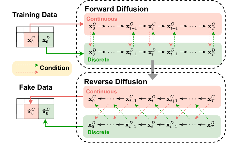
Figure 2: The overall workflow of co-evolving conditional diffusion models. Two diffusion models are connected by reading conditions from each other.

3.1 Co-evolving Conditional Diffusion Models

Fig. 2 shows an overall workflow of the co-evolving conditional diffusion models. Given a sample $\mathbf{x}_{0}$ which consists of mixed types of variables, we assume without loss of generality that $\mathbf{x}_{0}$ contains $N_{C}$ continuous columns $C=\{C_{1},C_{2},\dots,C_{N_{C}}\}$ and $N_{D}$ discrete columns $D=\{D_{1},D_{2},\dots,D_{N_{D}}\}$, where $\mathbf{x}_{0}=(\mathbf{x}_{0}^{C},\mathbf{x}_{0}^{D})$.

To synthesize samples from the space to which each type belongs, we train two diffusion models for the two variable types separately — however, the two diffusion models read conditions from each other since their diffusion/denoising processes are intercorrelated. We call them as continuous and discrete diffusion models, respectively. When training for continuous variables $\mathbf{x}_{0}^{C}$, we use the method described in Sec. 2.1.1. For discrete variables $\mathbf{x}_{0}^{D}$, the method in Sec. 2.1.2 is used.

To generate one related data pair with two models, we input each other’s output as a condition. The pair $(\mathbf{x}_{0}^{C},\mathbf{x}_{0}^{D})$ are then simultaneously perturbed at each forward time step $t$ in each space. To be specific, $\mathbf{x}_{t}^{C}$, which is the perturbed data in the continuous diffusion model, will be the condition of $\mathbf{x}_{t}^{D}$ in the discrete diffusion model, and vice versa. The model parameter $\theta_{C}$ (resp. $\theta_{D}$) is updated based on the following equations:

$$L_{\mathrm{Diff_{C}}}(\theta_{C})\coloneqq\mathbb{E}_{t,\mathbf{x}_{0}^{C},\boldsymbol{\epsilon}}\Big{[}\big{\|}\boldsymbol{\epsilon}-\boldsymbol{\epsilon}_{\theta_{C}}(\mathbf{x}_{t}^{C},t\mid\mathbf{x}_{t}^{D})\big{\|}^{2}\Big{]},$$ (10)

where $L_{\mathrm{Diff_{C}}}(\theta_{C})$ and $L_{\mathrm{Diff_{D}}}(\theta_{D})$ are the loss functions for the continuous and discrete diffusion models, respectively.

For the reverse process, generated samples, $\hat{\mathbf{x}}_{0}^{C}$ and $\hat{\mathbf{x}}_{0}^{D}$, are progressively synthesized from each noise space. The prior distributions of the two models are $p(\mathbf{x}_{T}^{C})=\mathcal{N}(\mathbf{x}_{T}^{C};\mathbf{0},\mathbf{I})$ and $p(\mathbf{x}_{T}^{D_{i}})=\mathcal{C}(\mathbf{x}_{T}^{D_{i}};{1/{K_{i}}})$, where $\{K_{i}\}_{i=1}^{N_{D}}$ is the number of categories of the discrete column $\{D_{i}\}_{i=1}^{N_{D}}$. After sampling noisy vectors, the two diffusion models convert the noises into fake samples while being conditioned on the denoised samples at the previous time step. In detail, to denoise one step from $\mathbf{x}_{t+1}^{C}$ (resp. $\mathbf{x}_{t+1}^{D}$) to $\mathbf{x}_{t}^{C}$ (resp. $\mathbf{x}_{t}^{D}$), the continuous diffusion model (resp. the discrete diffusion model) is conditioned both on the continuous sample $\mathbf{x}_{t+1}^{C}$ and discrete sample $\mathbf{x}_{t+1}^{D}$, which allows the collaboration of the two models to generate a related data record $\hat{\mathbf{x}}_{0}=(\hat{\mathbf{x}}_{0}^{C},\hat{\mathbf{x}}_{0}^{D}$).

Proposition 3.1.

The two forward processes of the continuous and discrete diffusion models are defined as follows:

$$q(\mathbf{x}_{t}^{C}|\mathbf{x}_{0}^{C})=\mathcal{N}(\mathbf{x}_{t}^{C};\sqrt{\bar{\alpha}_{t}}\mathbf{x}_{0}^{C},(1-\bar{\alpha}_{t})\mathbf{I}),$$ (12)

$$q(\mathbf{x}_{t}^{D_{i}}|\mathbf{x}_{0}^{D_{i}})=\mathcal{C}(\mathbf{x}_{t}^{D_{i}};\bar{\alpha}_{t}\mathbf{x}_{0}^{D_{i}}+(1-\bar{\alpha}_{t})/K_{i}),$$ (13)

where $1\leq i\leq N_{D}$, $\alpha_{t}\coloneqq 1-\beta_{t}$ and $\bar{\alpha}_{t}\coloneqq\prod_{i=1}^{t}{\alpha_{i}}$.

In addition, the reverse processes of the co-evolving conditional diffusion models are defined as follows:

$$p_{\theta_{C}}(\mathbf{x}_{0:T}^{C})\coloneqq p(\mathbf{x}_{T}^{C})\prod_{t=1}^{T}{p_{\theta_{C}}(\mathbf{x}_{t-1}^{C}|\mathbf{x}_{t}^{C},\mathbf{x}_{t}^{D})},$$ (14)

$$p_{\theta_{D}}(\mathbf{x}_{0:T}^{D_{i}})\coloneqq p(\mathbf{x}_{T}^{D_{i}})\prod_{t=1}^{T}{p_{\theta_{D}}(\mathbf{x}_{t-1}^{D_{i}}|\mathbf{x}_{t}^{D_{i}},\mathbf{x}_{t}^{C})},$$ (15)

where $1\leq i\leq N_{D}$ and the reverse transition probabilities are defined in Appendix C.

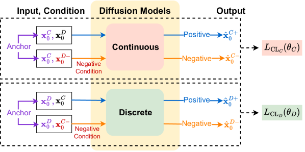
Figure 3: The proposed contrastive learning for tabular data. With a negative sampling method, we encourage the two diffusion models to generate samples that are closer to the positive samples and distinct from the negative samples.

3.2 Contrastive Learning

To connect the two diffusion models further, we adopt a contrastive learning method for tabular data by utilizing the following triplet loss (Schroff et al., 2015), which prefers positive samples to be close to the anchor. The objective function is as follows:

where $A$ is an anchor, $P$ is a positive sample, $N$ is a negative sample, $d$ is a distance metric, $m$ is a margin between the positive and negative samples, and $S$ is the number of samples.

Fig. 3 shows an overall process of the contrastive learning with the anchor, positive, and negative samples. Our contrastive learning process is applied to the continuous and discrete diffusion models separately. For simplicity but without loss of generality, we describe a process mainly for the continuous diffusion model, and the constrastive learning for the discrete diffusion model follows a similar process. In our method, we set a real sample $\mathbf{x}_{0}^{C}$ as the anchor, and a generated sample $\hat{\mathbf{x}}_{0}^{C+}$ conditioned on $\mathbf{x}_{0}^{D}$ as the positive sample. For the negative sample, we generate $\hat{\mathbf{x}}_{0}^{C-}$ with negative condition $\mathbf{x}_{0}^{D-}$, which is an inappropriate counterpart for $\mathbf{x}_{0}^{C}$.

Due to the computationally expensive nature of the diffusion models, generating a sample requires a long time, and for every training iteration, generating positive and negative samples for contrastive learning via $T$ steps may significantly delay training time. For this reason, we estimate the positive and negative samples using the model’s output. To be specific, we can predict $\hat{\mathbf{x}}_{0}^{C+}$ and $\hat{\mathbf{x}}_{0}^{C-}$ using the continuous diffusion model with the following equations:

$$\hat{\mathbf{x}}_{0}^{C+}=(\mathbf{x}_{t}^{C}-\sqrt{1-\bar{\alpha}_{t}}\boldsymbol{\epsilon}_{\theta_{C}}(\mathbf{x}_{t}^{C},t\mid\mathbf{x}_{t}^{D}))/\sqrt{\bar{\alpha}_{t}},$$ (17)

$$\hat{\mathbf{x}}_{0}^{C-}=(\mathbf{x}_{t}^{C}-\sqrt{1-\bar{\alpha}_{t}}\boldsymbol{\epsilon}_{\theta_{C}}(\mathbf{x}_{t}^{C},t\mid\mathbf{x}_{t}^{D-}))/\sqrt{\bar{\alpha}_{t}}.$$ (18)

Likewise, for the discrete diffusion model, we can directly estimate $\hat{\mathbf{x}}_{0}^{D+}$ and $\hat{\mathbf{x}}_{0}^{D-}$, using $p_{\theta_{D}}(\hat{\mathbf{x}}_{0}^{D+}|\mathbf{x}_{t}^{D},\mathbf{x}_{t}^{C})$ and $p_{\theta_{D}}(\hat{\mathbf{x}}_{0}^{D-}|\mathbf{x}_{t}^{D},\mathbf{x}_{t}^{C-})$, respectively.

After generating positive and negative samples, we calculate the contrastive learning losses with Eq. (16). For continuous variables $\mathbf{x}_{0}^{C}$ ($A$), $\hat{\mathbf{x}}_{0}^{C+}$ ($P$), and $\hat{\mathbf{x}}_{0}^{C-}$ ($N$), we use Euclidean distance as a metric $d$; for discrete variables $\mathbf{x}_{0}^{D}$ ($A$), $\hat{\mathbf{x}}_{0}^{D+}$ ($P$), and $\hat{\mathbf{x}}_{0}^{D-}$ ($N$), we use cross-entropy. Then, we combine the diffusion model losses and the contrastive learning losses as follows:

$$L_{\mathrm{C}}(\theta_{C})=L_{\mathrm{Diff_{C}}}(\theta_{C})+\lambda_{C}L_{\mathrm{CL_{C}}}(\theta_{C}),$$ (19)

$$L_{\mathrm{D}}(\theta_{D})=L_{\mathrm{Diff_{D}}}(\theta_{D})+\lambda_{D}L_{\mathrm{CL_{D}}}(\theta_{D}),$$ (20)

where $L_{\mathrm{CL}_{C}}(\theta_{C})$ and $L_{\mathrm{CL}_{D}}(\theta_{D})$ are the contrastive learning losses, and $L_{\mathrm{C}}(\theta_{C})$ and $L_{\mathrm{D}}(\theta_{D})$ are final losses for the continuous and discrete diffusion models, respectively, $0<\lambda_{C}<1$, and $0<\lambda_{D}<1$.

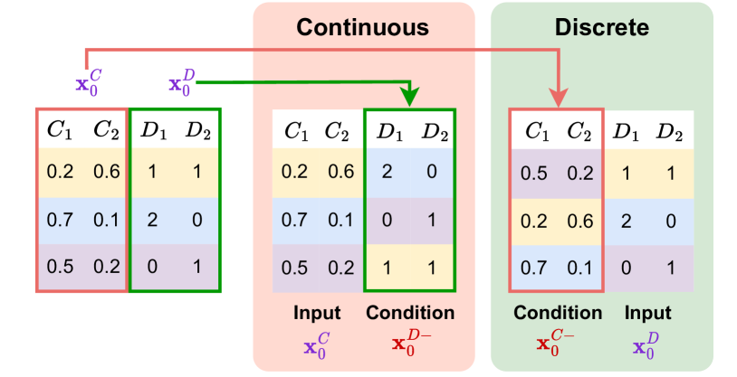
Figure 4: How to define the negative conditions. We randomly permute the continuous and discrete variable sets while maintaining their internal pairs and therefore, the inter-variable correlation does not make sense, i.e., they are not appropriate counterparts to each other.

Negative Condition We note that the negative conditions, $\mathbf{x}_{0}^{D-}$ and $\mathbf{x}_{0}^{C-}$, are the keys to generate the negative samples. To generate the negative samples, we focus on defining the negative conditions first. As shown in Fig. 4, we make the negative conditions by randomly shuffling the continuous and discrete variable sets so that they do not match. For example, given $\mathbf{x}_{0}^{C}$ of the continuous diffusion model, its negative condition $\mathbf{x}_{0}^{D-}$ is from other random record’s discrete part. The negative condition $\mathbf{x}_{0}^{C-}$ of $\mathbf{x}_{0}^{D}$ for the discrete diffusion model also follows the same method. In other words, the negative samples are generated by corrupting the inter-correlation between the continuous and discrete variable sets.

Algorithm 1 Training

  Initialize $\theta_{C}$ and $\theta_{D}$

  repeat

     $\mathbf{x}_{0}^{C}\sim q(\mathbf{x}_{0}^{C})$, $\mathbf{x}_{0}^{D}\sim q(\mathbf{x}_{0}^{D})$, $t\sim\mathcal{U}(\{1,\dots,T\})$

     Compute $L_{\mathrm{Diff_{C}}}(\theta_{C})$ and $L_{\mathrm{Diff_{D}}}(\theta_{D})$

     Make negative conditions $\mathbf{x}_{0}^{C-}$ and $\mathbf{x}_{0}^{D-}$

     Generate positive samples $\hat{\mathbf{x}}_{0}^{C+}$ and $\hat{\mathbf{x}}_{0}^{D+}$

     Generate negative samples $\hat{\mathbf{x}}_{0}^{C-}$ and $\hat{\mathbf{x}}_{0}^{D-}$

     Compute $L_{\mathrm{CL}_{C}}(\theta_{C})$ and $L_{\mathrm{CL}_{D}}(\theta_{D})$

     $L_{\mathrm{C}}(\theta_{C})\leftarrow L_{\mathrm{Diff_{C}}}(\theta_{C})+\lambda_{C}L_{\mathrm{CL_{C}}}(\theta_{C})$

     $L_{\mathrm{D}}(\theta_{D})\leftarrow L_{\mathrm{Diff_{D}}}(\theta_{D})+\lambda_{D}L_{\mathrm{CL_{D}}}(\theta_{D})$

     Update $\theta_{C}$ and $\theta_{D}$

  until converged

Algorithm 2 Sampling

  $\hat{\mathbf{x}}_{T}^{C}\sim p(\mathbf{x}_{T}^{C}),\hat{\mathbf{x}}_{T}^{D}\sim p(\mathbf{x}_{T}^{D})$

  for $i=T,\dots,1$ do

     $\hat{\mathbf{x}}_{i-1}^{C}\sim p_{\theta_{C}}(\hat{\mathbf{x}}_{i-1}^{C}|\hat{\mathbf{x}}_{i}^{C},\hat{\mathbf{x}}_{i}^{D})$

     $\hat{\mathbf{x}}_{i-1}^{D}\sim p_{\theta_{D}}(\hat{\mathbf{x}}_{i-1}^{D}|\hat{\mathbf{x}}_{i}^{D},\hat{\mathbf{x}}_{i}^{C})$

  end for

  return $\hat{\mathbf{x}}_{0}^{C},\hat{\mathbf{x}}_{0}^{D}$

3.3 Training & Sampling Algorithms

Algorithm 1 shows the overall training process of CoDi. We pre-process continuous variables to be $[-1,1]$ using the min-max scaler, and use one-hot encoding for discrete variables. Then, we initialize two diffusion model parameters $\boldsymbol{\theta}_{C}$ and $\boldsymbol{\theta}_{D}$. We sample $t$ from Uniform distribution, and train the two conditional diffusion models with Eqs. (10) and (11), respectively. After that, we make negative conditions for contrastive learning with the method described in Section 3.2. We generate positive and negative samples, and compute contrastive learning losses with Eq. (16). Finally, we integrate the contrastive learning losses with the diffusion model losses, and update model parameters $\boldsymbol{\theta}_{C}$ and $\boldsymbol{\theta}_{D}$, respectively.

The detailed sampling process of our method is in Algorithm 2. Firstly, we sample each noisy vector from the corresponding prior distribution, and convert the noises into fake samples through $T$ steps. At this point, $\mathbf{x}_{i-1}^{C}$ and $\mathbf{x}_{i-1}^{D}$ are conditioned on both denoised samples in continuous and discrete models at the previous time step $i$. After sampling, we post-process the continuous and discrete outputs, using the reverse scaler and Argmax function, respectively.

Table 1: Summarized experimental results in terms of sampling quality. We report averaged scores across the datasets. Full results are in Appendix E.1. We highlight the best results in light blue, and the second best with underline.

Methods	Binary				Multi-class				Regression
	Binary F1		AUROC		Macro F1		AUROC		$R^{2}$		RMSE
Identity	0.4154		0.8119		0.6514		0.8230		0.6673		0.3593
MedGAN	0.1523		0.5464		0.1537		0.5015		-inf		inf
VEEGAN	0.2591		0.5520		0.1206		0.5082		-inf		inf
CTGAN	0.3432		0.6745		0.2355		0.5546		-inf		inf
TVAE	0.3188		0.6867		0.2361		0.5974		-inf		inf
TableGAN	0.4078		0.7480		0.2715		0.6072		-0.0704		1.0015
OCT-GAN	0.3814		0.7350		0.3314		0.6434		-0.0868		1.0210
RNODE	0.3208		0.6651		0.3692		0.7037		-0.3037		1.1270
STaSy	0.4559		0.7961		0.6078		0.7997		-1.3200		1.2227
CoDi	0.4726		0.8106		0.6221		0.8026		0.4794		0.6477

4 Experiments

In this section, we introduce our experimental environments and results. We demonstrate the performance of our proposed method in terms of the generative learning trilemma. Detailed settings and hyperparameters are in Appendix D.

4.1 Experimental Setup

4.1.1 Datasets & Baselines

In our experiments, we select 11 datasets considering the number of continuous and discrete variables, and utilize 8 generative models from GANs to score-based generative models. Detailed information on datasets and baselines is in Appendix D.3 and D.4.

4.1.2 Evaluation Methods

We strictly follow evaluation methods described in Kim et al. (2022a). To evaluate the sampling quality, we train various classification/regression models with fake data, validate with real training data, and test them with real test data, called “TSTR” (Esteban et al., 2017; Jordon et al., 2019). We use F1 and AUROC as evaluation metrics for classification, and $R^{2}$ and RMSE for regression. We evaluate the model using 5 different fake samples by finding the best hyperparameter sets for classification/regression models. We test the best models with 5 fake samples and report the average score and standard deviation. To measure the sampling diversity, we utilize coverage (Naeem et al., 2020). For the sampling time, we measure wall-clock time taken to generate 10K fake samples. We measure the diversity and sampling time 5 times with different fake samples, and report their mean and standard deviation.

4.2 Experimental Results

4.2.1 Sampling Quality

In Table 1, we summarize experimental results on the sampling quality of each tabular data synthesis method. The results are averaged scores across the datasets. As shown, in classification tasks, MedGAN and VEEGAN show quite inferior performance to the others. More advanced GAN-based methods, i.e., TableGAN and OCT-GAN, and flow-based method, i.e., RNODE, perform to some degree. On the other hand, STaSy and CoDi show beyond-comparison results, especially, CoDi outperforms STaSy in all cases.

In the regression task, half of the baseline methods perform poorly, showing impractical results. Among the 9 methods, only CoDi shows positive $R^{2}$, which means CoDi is not only able to improve modeling in discrete variables but also generate high-quality continuous variables.

As shown in Fig. 5, the fake data by STaSy hardly follows the real data distribution. Especially in Fig. 5 (Right), STaSy generates an abnormal number of samples that belongs to a specific category, i.e., the second category from the left, while the fake data by CoDi has a similar histogram to the real data.

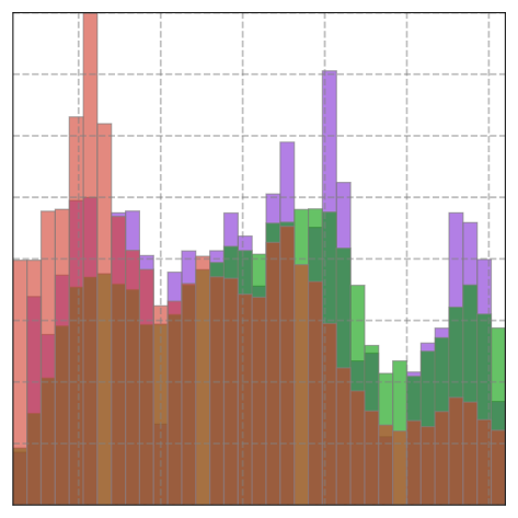
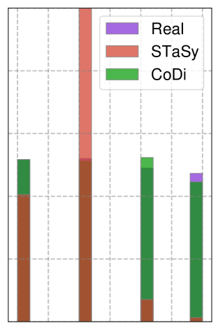
Figure 5: Comparison of column-wise distribution on real data, fake data by STaSy and CoDi. (Left) is for Days (continuous) of Bank and (Right) is for Seasons (discrete) of Absent.

4.2.2 Sampling Diversity

To evaluate the diversity of the fake data, we use coverage, which is the ratio of fake samples that have at least one real sample within their $5^{th}$ nearest neighborhoods. Table 3 shows the averaged coverage scores across the datasets. Among the baselines, MedGAN and VEEGAN show poor performance, whereas TableGAN and STaSy show reliable diversity to some extent. However, CoDi exceeds other methods and particularly performs well in multi-class classification and regression datasets, as shown in Tables 13 and 14 of Appendix E.2. In Stroke, TableGAN and CTGAN show good performance in terms of the sampling quality, however, CoDi outperforms by large margins in terms of the diversity.

Table 2: Summarized sampling diversity results. Full results are in Appendix E.2.

Methods	Coverage
MedGAN	0.0155
VEEGAN	0.0019
CTGAN	0.3834
TVAE	0.3903
TableGAN	0.5759
OCT-GAN	0.2547
RNODE	0.3841
STaSy	0.5771
CoDi	0.6931

Table 3: Summarized sampling time results. Full results are in Appendix E.3.

Methods	Runtime
MedGAN	0.0200
VEEGAN	0.0169
CTGAN	0.1260
TVAE	0.0140
TableGAN	0.0224
OCT-GAN	0.6008
RNODE	103.1449
STaSy	4.6417
CoDi	0.5187

Table 4: Experimental results on discrete data trained in continuous and discrete spaces. We report the F1 and coverage, and highlight the best results in bold.

Datasets	Continuous space			Discrete space
	F1 score	Coverage		F1 score	Coverage
Car	0.891±0.021	0.639±0.013		0.949±0.021	0.684±0.004
Clave	0.591±0.066	0.695±0.007		0.624±0.073	0.764±0.006
Nursery	0.780±0.016	0.553±0.002		0.823±0.036	0.568±0.003
Phishing	0.915±0.008	0.127±0.003		0.931±0.012	0.644±0.008

4.2.3 Sampling Time

In Table 3, we summarize sampling time. MedGAN and VEEGAN take short runtime, but show poor performance in terms of the sampling quality and diversity. Both TVAE and TableGAN also show fast speed, but the former generates less diverse samples, and the fake data by the latter shows low quality, which indicates they are not well-balanced in terms of the generative learning trilemma. However, STaSy and CoDi can sample in reliable runtime with high quality and diversity. Especially, CoDi shows about 9 times faster speed than that of STaSy, and is comparable to other GAN-based methods in terms of the sampling time.

In CoDi, the input dimensions of the models are decreased by using two diffusion models for the two variable types. Moreover, our network design for each diffusion model allows for reducing the learnable parameters by adapting the U-Net-based skip connection instead of residual blocks. As a result, the model’s complexity and training difficulty can be reduced considerably, and CoDi is able to balance the generative learning trilemma more.

4.3 Continuous vs. Discrete Spaces for Discrete Data

We claim that discrete variables should be treated in discrete spaces, unlike the existing methods that process them in continuous spaces along with continuous variables. To verify the claim, we examine which is the appropriate space for discrete variables by training them in continuous and discrete spaces. We introduce the following 4 datasets for experiments: Car, Clave, Nursery, and Phishing, which only contain discrete variables. More information is in Appendix D.3. The diffusion models for this experiment are the continuous and discrete diffusion models of CoDi, where the conditioning and contrastive learning are omitted.

As shown in Table 4, in all cases, the F1 and coverage scores of the fake data by the discrete diffision model are better than those of the continuous diffusion model. In Fig. 6, we compare the number of samples for each category of discrete columns between real data and fake data generated by the continuous and discrete diffusion models. As shown in Fig. 6 (Left), the continuous diffusion model fails to retain the real number of each category. Especially in Category 1 of Fig. 6 (Right), fake data by the continuous diffusion model generates more samples than the real data. The results show that the space where mixed-type variables are handled significantly affects the generation performance.

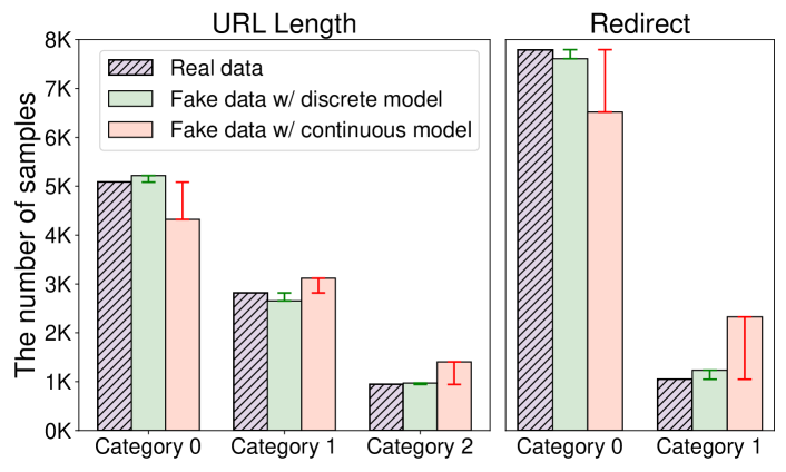
Figure 6: The number of samples for each category in discrete columns of Phishing. We selectively compare 2 columns (Left) URL Length, which has 3 categories, and (Right) Redirect, which is a binary class column. Green and red lines represent the gap between the real number of samples in each category and that of fake data.

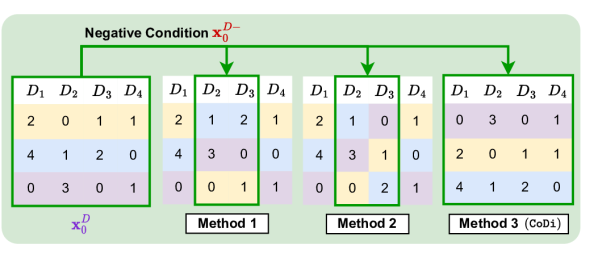
Figure 7: How to define negative conditions. Method 1 and Method 2 corrupt the inter-correlations between discrete variables, whereas Method 3 maintains them.

Table 5: Experimental results on 3 negative sampling methods. We report F1 for classification data, $R^{2}$ for regression data, and coverage. The best results are highlighted in bold.

Methods	Metrics	Heart	Faults	Insurance
Method 1	F1 ($R^{2}$)	0.857±0.048	0.699±0.041	(0.567±0.343)
	Coverage	0.847±0.028	0.191±0.012	0.128±0.020
Method 2	F1 ($R^{2}$)	0.850±0.039	0.709±0.042	(0.554±0.402)
	Coverage	0.820±0.022	0.247±0.005	0.189±0.024
Method 3	F1 ($R^{2}$)	0.872±0.039	0.715±0.046	(0.575±0.398)
(CoDi)	Coverage	0.949±0.012	0.270±0.017	0.262±0.020

4.4 Negative Sampling Methods

Since the contrastive learning for tabular data has rarely been studied, in this section, we provide a comparison of possible negative sampling methods in terms of the sampling quality and diversity. We define 3 methods for the negative condition, as shown in Fig. 7. Let us define the discrete condition for the continuous diffusion model first for convenience. Firstly, for Method 1 and Method 2, we randomly select two columns from discrete variables for the negative condition. Then, we shuffle the rows of the two columns, for Method 1, retaining the pair of the two columns, and for Method 2, without maintaining the pair of columns. For Method 3, which is our proposed method, we shuffle the rows of discrete variables altogether, maintaining the pair. The continuous condition can be defined by following the same process.

In Table 5, we compare the negative sampling methods. Although all negative sampling methods show reasonable performance in our experiment with 3 datasets, Method 3 shows the best performance in terms of the sampling quality and diversity. The first two methods disrupt not only the relationship between continuous and discrete variables but also the inter-correlations between each variable type, increasing the training difficulty of the model. On the other hand, Method 3 retains the latter, which can result in the outcome.

Fig. 8 presents the training loss curves of the contrastive learning. As shown, the loss curves of the first two methods fluctuate drastically, while the loss curves of Method 3 converges stably, which represents the easiness of training.

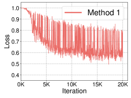
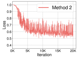
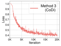
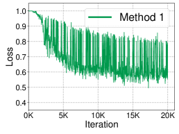
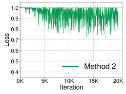
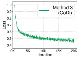
Figure 8: The training loss curves of triplet loss with respect to the negative sampling method in Faults. Red and green lines mean $L_{\mathrm{CL_{C}}}(\theta_{C})$ and $L_{\mathrm{CL_{D}}}(\theta_{D})$, respectively. (Left) are for Method 1, (Middle) are for Method 2, and (Right) are for Method 3.

Table 6: Ablation study on the efficacy of the contrastive learning. We report F1 for classification data, $R^{2}$ for regression data, and coverage.

Datasets	CoDi w/o CL			CoDi
	F1 ($R^{2}$)	Coverage		F1 ($R^{2}$)	Coverage
Bank	0.527±0.032	0.699±0.003		0.566±0.014	0.687±0.002
Heart	0.886±0.043	0.879±0.017		0.872±0.039	0.949±0.012
Seismic	0.210±0.064	0.380±0.016		0.305±0.040	0.359±0.005
Stroke	0.129±0.036	0.651±0.020		0.147±0.016	0.919±0.008
CMC	0.484±0.024	0.932±0.011		0.503±0.008	0.934±0.015
Customer	0.350±0.008	0.789±0.019		0.352±0.015	0.833±0.021
Faults	0.705±0.047	0.272±0.016		0.715±0.046	0.270±0.017
Obesity	0.912±0.038	0.777±0.018		0.919±0.034	0.742±0.015
Absent	(-0.026±0.036)	0.801±0.009		(0.095±0.022)	0.843±0.023
Drug	(0.748±0.074)	0.813±0.013		(0.768±0.049)	0.827±0.046
Insurance	(0.531±0.308)	0.218±0.028		(0.575±0.398)	0.262±0.020

4.5 Ablation Study on Contrastive Learning

As shown in Table 6, we conduct ablation experiments to show the efficacy of the contrastive learning on CoDi. ‘CoDi w/o CL’ means the model trained without contrastive learning. In Bank, Seismic, Faults, and Obesity, the contrastive learning improves F1 scores, and in Heart, it significantly enhances the sampling diversity. In other datasets, it enhances not only the sampling quality but also diversity. The results demonstrate that the design choice of the anchor, positive, and negative samples is reasonable and the contrastive learning is properly performed to synthesize a better sample.

5 Conclusions

Synthesizing realistic tabular data is one of the utmost tasks as tabular data is a frequently used data format. However, modeling tabular data is of non-trivial due to the nature of tabular data, which consists of mixed data types. To this end, we introduce the set of diffusion models for continuous and discrete variables. By conditioning the diffusion models at every training iteration using each other’s outputs, the models are able to co-evolve maintaining the correlation of continuous and discrete variables. Moreover, the binding between two models is further reinforced by bringing the contrastive learning to our training.

In our experiments with 11 real-world benchmark datasets and 8 baselines, CoDi outperforms others in terms of sampling quality and diversity. Compared to STaSy, the recent state-of-the-art tabular data synthesis method, our method improves the sampling time by about 90%, owing to the reduced training difficulty. Consequently, CoDi achieves well-balanced generative learning trilemma, representing remarkable advancements in tabular data synthesis.

Limitations CoDi is designed for better learning of continuous and discrete variables simultaneously, which means that our method may not be applicable when there are only continuous or discrete variables. However, real-world tabular data typically has mixed types.

Societal impacts As the generated fake data become realistic, there is a risk of being abused by people trying to achieve their immoral purposes. This leads to the research topic of protecting privacy in generative models being actively studied (Lee et al., 2021; Hyeong et al., 2022).

Appendix A Preliminary Experiment

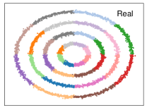
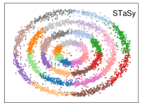
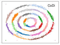
Figure 9: Preliminary experiment on a toy dataset

In Fig. 9, we provide detailed visualizations for the preliminary experiment on the toy dataset. The dataset contains 4 columns. The x-axis and y-axis are continuous variables, while the 16 colors and which circle the sample belongs to are discrete variables. As shown, fake data by CoDi is more similar to real data than fake data by STaSy. Specifically, fake data by STaSy fails to generate continuous and discrete variables precisely, resulting in noisy samples at the class boundaries.

Appendix B Network Architecture

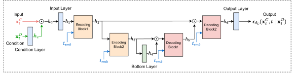
Figure 10: The continuous diffusion model network architecture diagram. The proposed continuous diffusion model network architecture is a modification of U-Net. We use the fully connected layers, and adopt the skip connection to pass the features from encoder to decoder. The continuous diffusion model is conditioned on discrete variables $\mathbf{x}_{t}^{D}$ and time $t$.

Our proposed two diffusion model’s network is U-Net-based architecture. We introduce an architecture only for the continuous diffusion model, but the same architecture is used for the discrete diffusion model. In Fig. 10, $\mathbf{x}_{t}^{C}$ is an input, $\mathbf{x}_{t}^{D}$ is a condition, $\odot$ is a concatenation operator, and $\boldsymbol{\epsilon}_{\theta_{C}}$ is an output of the continuous diffusion model. We use 4 layers; input, condition, bottom, and output layers, and 4 blocks; 2 encoding blocks and 2 decoding blocks linked together via a skip connection. The time $t$ is conditioned on the encoding and decoding blocks, and $t_{emb}$ is defined as follows:

$$t_{emb}=\mathtt{FC}_{emb}^{2}(\mathtt{ReLU}(\mathtt{FC}_{emb}^{1}(\mathtt{Emb}(t)))),$$ (21)

where $\mathtt{Emb}$ is a sinusoidal positional embedding (Vaswani et al., 2017), and $\mathtt{FC}$ is a fully connected layer. The condition layer inputs the condition $\mathbf{x}_{t}^{D}$ and outputs a hidden vector $h_{c}$, which has the dimension of half of the $\mathbf{x}_{t}^{C}$. Given the input $\mathbf{x}_{t}^{C}$ and the hidden vector $h_{c}$, we design the following continuous diffusion model $\boldsymbol{\epsilon}_{\theta_{C}}(\mathbf{x}_{t}^{C},t\mid\mathbf{x}_{t}^{D})$:

$$h_{c} =\mathtt{FC}_{c}(\mathbf{x}_{t}^{D}),$$ (22)

$$h_{0} =\mathbf{x}_{t}^{C}\odot h_{c},$$

$$h_{1} =\mathtt{FC}_{1}(h_{0}),$$

$$h_{i} =\mathtt{ReLU}(\mathtt{FC}_{i}^{2}(\mathtt{ReLU}(\mathtt{FC}_{i}^{1}(h_{i-1}))\oplus\mathtt{ReLU}(\mathtt{FC}_{i}^{t}(t_{emb})))), i=2,3,$$ if

$$h_{4} =\mathtt{ReLU}(\mathtt{FC}_{4}(h_{3})),$$

$$h_{i} =\mathtt{ReLU}(\mathtt{FC}_{i}^{2}(\mathtt{ReLU}(\mathtt{FC}_{i}^{1}(h_{i-1}\odot h_{8-i}))\oplus\mathtt{ReLU}(\mathtt{FC}_{i}^{t}(t_{emb})))), i=5,6,$$ if

$$\boldsymbol{\epsilon}_{\theta_{C}}(\mathbf{x}_{t}^{C},t\mid\mathbf{x}_{t}^{D}) =\mathtt{FC}_{7}(h_{6}),$$

where $\odot$ means the concatenation operator, $h_{i}$ is the $i^{th}$ hidden vector, and $\oplus$ means the element-wise addition.

Appendix C The Reverse Transition Probabilities for the Co-evolving Conditional Diffusion models

In Proposition 3.1, we define the forward and reverse processes of the co-evolving conditional diffusion models.

The reverse transition probabilities of each reverse process are defined as follows:

$$p_{\theta_{C}}(\mathbf{x}_{t-1}^{C}|\mathbf{x}_{t}^{C},\mathbf{x}_{t}^{D})=\mathcal{N}(\mathbf{x}_{t-1}^{C};\boldsymbol{\mu}_{\theta_{C}}(\mathbf{x}_{t}^{C},t\mid\mathbf{x}_{t}^{D}),\sigma_{t}^{2}\mathbf{I}),$$ (23)

$$p_{\theta_{D}}(\mathbf{x}_{t-1}^{D_{i}}|\mathbf{x}_{t}^{D_{i}},\mathbf{x}_{t}^{C})=\mathcal{C}(\mathbf{x}_{t-1}^{D_{i}};\mathbf{p}^{i}_{\theta_{D}}),$$ (24)

where $1\leq i\leq N_{D}$, and $\boldsymbol{\mu}_{\theta_{C}}(\mathbf{x}_{t}^{C},t\mid\mathbf{x}_{t}^{D})$, $\sigma_{t}^{2}$, and $\mathbf{p}^{i}_{\theta_{D}}$ are defined as follows:

$$\boldsymbol{\mu}_{\theta_{C}}(\mathbf{x}_{t}^{C},t\mid\mathbf{x}_{t}^{D})=\frac{1}{\sqrt{\alpha_{t}}}(\mathbf{x}_{t}^{C}-\frac{\beta_{t}}{\sqrt{1-\bar{\alpha}_{t}}}\boldsymbol{\epsilon}_{\theta_{C}}(\mathbf{x}_{t}^{C},t\mid\mathbf{x}_{t}^{D})),$$ (25)

$$\sigma_{t}^{2}=\frac{1-\bar{\alpha}_{t-1}}{1-\bar{\alpha}_{t}}\beta_{t}\mathbf{I},$$ (26)

$$\mathbf{p}^{i}_{\theta_{D}}=\sum_{\hat{\mathbf{x}}_{0}^{D_{i}}=1}^{K_{i}}q(\mathbf{x}_{t-1}^{D_{i}}|\mathbf{x}_{t}^{D_{i}},\hat{\mathbf{x}}_{0}^{D_{i}})p_{\theta_{D}}(\hat{\mathbf{x}}_{0}^{D_{i}}|\mathbf{x}_{t}^{D_{i}},\mathbf{x}_{t}^{C}).$$ (27)

Appendix D Detailed Experimental Settings for Reproducibility

D.1 Experimental Environments

Our software and hardware environments are as follows: Ubuntu 18.04.6 LTS, Python 3.10.8, Pytorch 1.11.0, CUDA 11.7, and NVIDIA Driver 470.161.03, i9, CPU, and NVIDIA RTX 3090.

D.2 Hyperparameter Settings for CoDi

Hyperparameter settings for the best models are summarized in Tables 7 and 8. We use a learning rate in {2e-03, 2e-05}. We search for $\dim(\mathtt{Emb}(t))$, which is a time embedding dimension for every block consisting of network, in {16, 32, 64, 128} for each diffusion model. $\dim(h_{1}),\dim(h_{2}),$ and $\dim(h_{3})$ decide the number of learnable parameters for networks, where $\dim(h_{1})=\dim(h_{6})$, $\dim(h_{2})=\dim(h_{5})$, and $\dim(h_{3})=\dim(h_{4})$, allowing the encoder and decoder part to be symmetry. We search for {$\dim(h_{1}),\dim(h_{2}),\dim(h_{3})$} in {{16, 32, 64}, {32, 64, 128}, {64, 128, 256}, {128, 256, 512}}, considering the dataset size. The constrastive learning loss coefficient $\lambda_{C}$ and $\lambda_{D}$ are {0.2, 0.3, …, 0.7, 0.8}. We use a linear noise schedule for $\beta_{t}$, which is linearly increased from 1e-05 to 2e-02, and use the total diffusion timesteps as $T=50$.

Table 7: The best hyperparameters used in Tables 1, 3, and 3 for the continuous diffusion model

Datasets	Continuous diffusion model
	Learning rate	$\dim(\mathtt{Emb}(t))$	$\dim(h_{1}),\dim(h_{2}),\dim(h_{3})$	$\lambda_{C}$
Bank	2e-03	32	64,128,256	0.2
Heart	2e-03	16	64,128,256	0.2
Seismic	2e-03	64	64,128,256	0.4
Stroke	2e-05	16	64,128,256	0.2
CMC	2e-03	32	16,32,64	0.6
Customer	2e-03	16	32,64,128	0.2
Faults	2e-03	32	64,128,256	0.2
Obesity	2e-03	64	64,128,256	0.5
Absent	2e-03	32	64,128,256	0.3
Drug	2e-03	32	64,128,256	0.2
Insurance	2e-03	32	64,128,256	0.2

Table 8: The best hyperparameters used in Tables 1, 3, and 3 for the discrete diffusion model

Datasets	Discrete diffusion model
	Learning rate	$\dim(\mathtt{Emb}(t))$	$\dim(h_{1}),\dim(h_{2}),\dim(h_{3})$	$\lambda_{D}$
Bank	2e-03	64	64,128,256	0.3
Heart	2e-03	64	64,128,256	0.2
Seismic	2e-03	64	64,128,256	0.6
Stroke	2e-03	128	128,256,512	0.3
CMC	2e-03	32	32,64,128	0.8
Customer	2e-03	64	32,64,128	0.5
Faults	2e-03	64	64,128,256	0.2
Obesity	2e-03	64	64,128,256	0.3
Absent	2e-05	32	64,128,256	0.2
Drug	2e-03	32	64,128,256	0.2
Insurance	2e-03	32	128,256,512	0.2

D.3 Datasets

In this section, we provide the real-world datasets used for our experiments. The datasets are selected considering the number of continuous and discrete variables consisting of the tabular data. Table 9 summarizes the statistical information of the datasets.

Table 9: Dataset information used in our experiments. #Train and #Test are the numbers of training data and test data, respectively, and $N_{C}$ and $N_{D}$ are the numbers of continuous and discrete columns, respectively.

Task	Datasets	#Train	#Test	$N_{C}$	$N_{D}$
Binary	Bank	36169	9042	7	10
	Heart	815	203	4	10
	Seismic	2068	516	11	5
	Stroke	2740	685	2	8
	Phishing	8844	2211	0	31
Multi-class	CMC	1179	294	2	8
	Customer	800	200	5	7
	Faults	1553	388	24	4
	Obesity	1689	422	8	9
	Car	1383	345	0	7
	Clave	8639	2159	0	17
	Nursery	10368	2592	0	9
Regression	Absent	592	148	12	9
	Drug	829	207	5	1
	Insurance	789	197	3	8

• Bank (Moro et al., 2014) is to predict whether a client subscribed a term deposit or not. The dataset contains personal financial situations, e.g., whether the person has housing loan or not. (https://archive.ics.uci.edu/ml/datasets/bank+marketing) (CC BY 4.0)

• Heart is to predict the presence of heart disease in a patient, which consists of personal health condition. (https://www.kaggle.com/datasets/johnsmith88/heart-disease-dataset) (CC BY 4.0)

• Seismic (Sikora et al., 2010) predicts the impact of an earthquake. The dataset contains seismic information such as the number of seismic bumps. (https://archive.ics.uci.edu/ml/datasets/seismic-bumps) (CC BY 4.0)

• Stroke (Liu et al., 2019) is used to predict whether a patient is likely to get stroke based on the patient information. (CC0 1.0) (https://www.kaggle.com/datasets/fedesoriano/stroke-prediction-dataset)

• Phishing (Mohammad et al., 2012) is to predict if a webpage is a phishing site. The dataset consists of important features for predicting the phishing sites, including information about webpage transactions. (https://archive.ics.uci.edu/ml/datasets/phishing+websites) (CC BY 4.0)

• CMC (Lim et al., 2000) is to predict the current contraceptive method chioce of a woman based on her demographic and socio-economic characteristics. (https://archive.ics.uci.edu/ml/datasets/Contraceptive+Method+Choice) (CC BY 4.0)

• Customer consists of information about the telecommunication company’s customers and their groups. (https://www.kaggle.com/prathamtripathi/customersegmentation) (CC0 1.0)

• Faults (provided by Semeion, 2019) is for fault detection in steel manufacturing process. (https://archive.ics.uci.edu/ml/datasets/steel+plates+faults) (CC BY 4.0)

• Obesity (Palechor & de la Hoz Manotas, 2019) is to estimate the obesity level based on eating habits and physical condition of individuals from Mexico, Peru, and Columbia. (https://archive.ics.uci.edu/ml/datasets/Estimation+of+obesity+levels+based+on+eating+habits+and+physical+condition+) (CC BY 4.0)

• Car (Bohanec & Rajkovic, 1988) is to categorize a car condition, which contains car characteristics, such as the number of doors. (https://archive.ics.uci.edu/ml/datasets/Car+Evaluation) (CC BY 4.0)

• Clave (Vurkaç, 2012) is to predict the class to which input music belongs. The class is one of the Neutral, Reverse Clave, Forward Clave, and Incoherent. (https://archive.ics.uci.edu/ml/datasets/Firm-Teacher_Clave-Direction_Classification) (CC BY 4.0)

• Nursery (Olave et al., 1989) is to rank applications for nursery schools. The dataset contains the family structures, parents’ occupation, children’s health condition, and so on. (https://archive.ics.uci.edu/ml/datasets/nursery) (CC BY 4.0)

• Absent (Martiniano et al., 2012) predicts the absenteeism time in hours. The dataset consists demographic information. (https://archive.ics.uci.edu/ml/datasets/Absenteeism+at+work) (CC BY 4.0)

• Drug (OECD, 2021) covers expenditure on prescription medicines and self-medication. (https://data.oecd.org/healthres/pharmaceutical-spending.htm) (CC BY-NC-SA 3.0 IGO)

• Insurance is for prediction on the yearly medical cover cost. The dataset contains a person’s medical information. (https://www.kaggle.com/datasets/tejashvi14/medical-insurance-premium-prediction) (CC0 1.0)

D.4 Baselines

We describe the baseline methods used in our experiment. The baseline methods are as follows, which consist of various types of generative models, from the GAN-based methods to the score-based generative model.

• MedGAN (Choi et al., 2017) includes non-adversarial losses for discrete medical records.

• VEEGAN (Srivastava et al., 2017) is a GAN equipped with a reconstructor network, which aims for diverse sampling.

• CTGAN and TVAE (Xu et al., 2019) handle challenges from the mixed type of variables.

• TableGAN (Park et al., 2018) is a GAN for tabular data using convolutional neural networks.

• OCT-GAN (Kim et al., 2021) contains neural networks based on neural ordinary differential equations.

• RNODE (Finlay et al., 2020) is an advanced flow-based model for image data, and we customize the network to synthesize tabular data.

• STaSy (Kim et al., 2022a) is a currently proposed score-based generative model for tabular data synthesis.

Appendix E Additional Experimental Results

E.1 Sampling Quality

We consider F1 and AUROC (resp. $R^{2}$ and RMSE) for the classification (resp. regression) tasks to evaluate the sampling quality. Full results for all datasets and baselines are in Tables 10 and 11 for classification, and in Table 12 for regression. For reliability, we report their mean and standard deviation of 5 evaluations on TSTR evaluation. Identity is a case of “TRTR”, where we train classification/regression models with real training data and test them on real test data. As shown, CoDi outperforms the others in almost all cases. Especially in the regression task, CoDi is the only method that shows the positive $R^{2}$ in all datasets.

Table 10: Binary classification results with real data. We report binary F1 and AUROC for binary classification.

Methods	Bank			Heart			Seismic			Stroke
	Binary F1	AUROC		Binary F1	AUROC		Binary F1	AUROC		Binary F1	AUROC
Identity	0.520±0.038	0.895±0.080		0.972±0.057	0.990±0.025		0.102±0.109	0.697±0.055		0.068±0.042	0.666±0.085
MedGAN	0.000±0.000	0.500±0.000		0.594±0.067	0.659±0.061		0.000±0.000	0.500±0.000		0.015±0.027	0.527±0.022
VEEGAN	0.206±0.015	0.521±0.061		0.525±0.126	0.453±0.114		0.161±0.020	0.590±0.050		0.144±0.052	0.644±0.026
CTGAN	0.515±0.029	0.883±0.022		0.611±0.015	0.543±0.040		0.088±0.054	0.655±0.061		0.159±0.022	0.617±0.028
TVAE	0.524±0.019	0.870±0.025		0.745±0.056	0.843±0.069		0.000±0.000	0.500±0.000		0.006±0.015	0.534±0.021
TableGAN	0.444±0.060	0.812±0.074		0.767±0.023	0.868±0.039		0.219±0.056	0.679±0.043		0.201±0.015	0.634±0.019
OCT-GAN	0.539±0.019	0.887±0.020		0.649±0.033	0.733±0.056		0.209±0.025	0.686±0.077		0.128±0.020	0.634±0.041
RNODE	0.263±0.043	0.739±0.083		0.811±0.037	0.895±0.041		0.141±0.044	0.515±0.081		0.068±0.011	0.511±0.019
STaSy	0.562±0.022	0.905±0.017		0.835±0.031	0.918±0.025		0.295±0.019	0.721±0.032		0.132±0.018	0.641±0.049
CoDi	0.566±0.014	0.894±0.023		0.872±0.039	0.934±0.038		0.305±0.040	0.731±0.036		0.147±0.016	0.684±0.015

Table 11: Multi-class classification results with real data. We report macro F1 and AUROC for multi-class classification.

Methods	CMC			Customer			Faults			Obesity
	Macro F1	AUROC		Macro F1	AUROC		Macro F1	AUROC		Macro F1	AUROC
Identity	0.493±0.009	0.709±0.011		0.370±0.022	0.669±0.021		0.777±0.052	0.923±0.048		0.965±0.014	0.992±0.015
MedGAN	0.296±0.015	0.513±0.008		0.210±0.043	0.493±0.030		0.068±0.000	0.500±0.000		0.040±0.000	0.500±0.000
VEEGAN	0.287±0.036	0.533±0.009		0.105±0.000	0.500±0.000		0.050±0.000	0.500±0.000		0.040±0.000	0.500±0.000
CTGAN	0.335±0.012	0.514±0.017		0.247±0.013	0.521±0.011		0.221±0.025	0.661±0.073		0.139±0.014	0.522±0.024
TVAE	0.297±0.004	0.537±0.026		0.140±0.006	0.518±0.005		0.068±0.000	0.500±0.000		0.439±0.024	0.835±0.016
TableGAN	0.366±0.016	0.582±0.024		0.241±0.007	0.512±0.005		0.187±0.017	0.593±0.047		0.292±0.008	0.741±0.041
OCT-GAN	0.345±0.019	0.541±0.034		0.227±0.015	0.493±0.003		0.357±0.004	0.796±0.049		0.396±0.061	0.744±0.085
RNODE	0.394±0.026	0.610±0.038		0.315±0.027	0.600±0.036		0.298±0.056	0.778±0.085		0.469±0.062	0.826±0.068
STaSy	0.492±0.010	0.686±0.027		0.337±0.002	0.635±0.044		0.668±0.022	0.894±0.039		0.900±0.034	0.984±0.019
CoDi	0.503±0.008	0.694±0.013		0.352±0.015	0.619±0.036		0.715±0.046	0.908±0.040		0.919±0.034	0.989±0.012

Table 12: Regression results with real data. We report $R^{2}$ and RMSE for regression.

Methods	Absent			Drug			Insurance
	$R^{2}$	RMSE		$R^{2}$	RMSE		$R^{2}$	RMSE
Identity	0.352±0.072	0.795±0.044		0.992±0.009	0.128±0.095		0.658±0.317	0.155±0.068
MedGAN	-inf	inf		-4.877±1.800	4.170±0.708		-inf	inf
VEEGAN	-8.802±5.721	2.912±1.209		-5.354±3.583	4.195±1.452		-inf	inf
CTGAN	-inf	inf		0.034±0.080	1.705±0.072		-0.196±0.308	0.307±0.038
TVAE	-inf	inf		-inf	inf		-inf	inf
TableGAN	-0.363±0.116	1.152±0.049		0.183±0.141	1.567±0.132		-0.031±0.290	0.285±0.038
OCT-GAN	-0.123±0.064	1.046±0.030		0.019±0.129	1.713±0.115		-0.156±0.220	0.303±0.027
RNODE	-0.604±0.285	1.246±0.108		-0.174±0.712	1.838±0.127		-0.133±0.160	0.297±0.084
STaSy	-4.833±2.768	2.303±0.629		0.568±0.134	1.131±0.181		0.306±0.129	0.235±0.022
CoDi	0.095±0.022	0.940±0.012		0.768±0.049	0.832±0.088		0.575±0.398	0.171±0.074

E.2 Sampling Diversity

To evaluate the sampling diversity of fake data, we consider coverage (Naeem et al., 2020). Full results are in Tables 13, 14 and 15. We measure the coverage 5 times with different fake data by each method and report their mean and standard deviation. CoDi shows comparable performance in terms of the sampling diversity to the original data in many cases.

Table 13: Sampling diversity in terms of coverage on binary classification datasets

Methods	Bank	Heart	Seismic	Stroke
MedGAN	0.000±0.000	0.090±0.011	0.000±0.000	0.010±0.001
VEEGAN	0.001±0.000	0.004±0.000	0.000±0.000	0.000±0.000
CTGAN	0.774±0.001	0.098±0.010	0.341±0.013	0.664±0.015
TVAE	0.783±0.003	0.287±0.010	0.401±0.009	0.610±0.016
TableGAN	0.623±0.004	0.816±0.031	0.553±0.011	0.896±0.008
OCT-GAN	0.623±0.004	0.004±0.000	0.326±0.015	0.594±0.014
RNODE	0.403±0.003	0.679±0.034	0.198±0.010	0.251±0.010
STaSy	0.854±0.012	0.839±0.009	0.505±0.017	0.789±0.021
CoDi	0.687±0.002	0.949±0.012	0.359±0.005	0.919±0.008

Table 14: Sampling diversity in terms of coverage on multi-class classification datasets

Methods	CMC	Customer	Faults	Obesity
MedGAN	0.012±0.004	0.015±0.001	0.002±0.000	0.000±0.000
VEEGAN	0.000±0.000	0.003±0.000	0.002±0.000	0.000±0.000
CTGAN	0.715±0.008	0.428±0.013	0.031±0.005	0.275±0.008
TVAE	0.603±0.014	0.398±0.010	0.149±0.007	0.359±0.010
TableGAN	0.766±0.018	0.896±0.013	0.205±0.020	0.348±0.011
OCT-GAN	0.303±0.011	0.073±0.009	0.054±0.007	0.299±0.006
RNODE	0.869±0.015	0.723±0.024	0.138±0.007	0.313±0.008
STaSy	0.943±0.007	0.713±0.025	0.202±0.014	0.633±0.007
CoDi	0.934±0.015	0.833±0.021	0.270±0.017	0.742±0.015

Table 15: Sampling diversity in terms of coverage on regression datasets

Methods	Absent	Drug	Insurance
MedGAN	0.015±0.001	0.009±0.002	0.018±0.005
VEEGAN	0.002±0.000	0.002±0.000	0.008±0.000
CTGAN	0.287±0.012	0.557±0.018	0.048±0.005
TVAE	0.082±0.009	0.588±0.018	0.034±0.011
TableGAN	0.294±0.017	0.880±0.019	0.059±0.018
OCT-GAN	0.044±0.007	0.460±0.021	0.023±0.004
RNODE	0.085±0.007	0.395±0.018	0.172±0.014
STaSy	0.004±0.003	0.662±0.016	0.206±0.016
CoDi	0.843±0.023	0.827±0.046	0.262±0.020

E.3 Sampling Time

Tables 16, 17 and 18 summarize the sampling time evaluation results. We measure the wall-clock time taken to sample 10K fake records 5 times and report their mean and standard deviation. TableGAN and TVAE show fast sampling time in almost all cases, while RNODE takes the longest time. CoDi shows much faster sampling time compared to STaSy, which is state-of-the-art score-based generative model.

Table 16: We summarize the sampling time for each binary classification dataset and tabular data synthesis method.

Methods	Bank	Heart	Seismic	Stroke
MedGAN	0.019±0.000	0.019±0.000	0.019±0.000	0.019±0.000
VEEGAN	0.016±0.000	0.018±0.001	0.017±0.001	0.017±0.002
CTGAN	0.138±0.000	0.110±0.001	0.138±0.000	0.101±0.001
TVAE	0.014±0.001	0.012±0.000	0.011±0.000	0.012±0.000
TableGAN	0.058±0.002	0.005±0.000	0.005±0.000	0.007±0.000
OCT-GAN	0.477±0.001	0.467±0.001	0.576±0.000	0.829±0.000
RNODE	229.254±3.280	95.677±1.838	35.550±0.839	230.209±0.771
STaSy	2.069±0.004	7.501±1.457	3.230±0.150	3.357±0.108
CoDi	1.321±0.022	0.600±0.240	0.259±0.014	0.793±0.417

Table 17: We summarize the sampling time for each multi-class classification dataset and tabular data synthesis method.

Methods	CMC	Customer	Faults	Obesity
MedGAN	0.019±0.000	0.030±0.000	0.019±0.000	0.019±0.001
VEEGAN	0.016±0.001	0.015±0.000	0.022±0.001	0.018±0.001
CTGAN	0.125±0.000	0.134±0.000	0.158±0.000	0.126±0.006
TVAE	0.011±0.000	0.011±0.000	0.013±0.000	0.014±0.001
TableGAN	0.007±0.000	0.006±0.000	0.029±0.000	0.059±0.002
OCT-GAN	0.744±0.329	0.606±0.070	0.462±0.008	0.457±0.002
RNODE	32.930±0.279	36.931±0.394	52.887±1.810	85.399±0.542
STaSy	1.952±0.007	5.111±0.224	2.063±0.024	2.051±0.027
CoDi	0.306±0.019	0.290±0.019	0.241±0.012	0.403±0.044

Table 18: We summarize the sampling time for each regression dataset and tabular data synthesis method.

Methods	Absent	Drug	Insurance
MedGAN	0.020±0.001	0.019±0.000	0.019±0.000
VEEGAN	0.021±0.001	0.013±0.001	0.014±0.000
CTGAN	0.149±0.001	0.103±0.000	0.104±0.000
TVAE	0.023±0.000	0.012±0.000	0.021±0.000
TableGAN	0.061±0.001	0.005±0.000	0.005±0.000
OCT-GAN	0.583±0.005	0.703±0.000	0.704±0.000
RNODE	220.460±1.814	43.188±0.480	72.110±0.331
STaSy	16.908±0.062	2.965±0.225	3.849±3.015
CoDi	0.764±0.383	0.269±0.016	0.460±0.001

References

- Austin et al. (2021) Austin, J., Johnson, D. D., Ho, J., Tarlow, D., and van den Berg, R. Structured denoising diffusion models in discrete state-spaces. Advances in Neural Information Processing Systems, 34:17981–17993, 2021.
- Aviñó et al. (2018) Aviñó, L., Ruffini, M., and Gavaldà, R. Generating synthetic but plausible healthcare record datasets, 2018.
- Bohanec & Rajkovic (1988) Bohanec, M. and Rajkovic, V. Knowledge acquisition and explanation for multi-attribute decision making. In 8th intl workshop on expert systems and their applications, pp. 59–78. Avignon France, 1988.
- Borisov et al. (2021) Borisov, V., Leemann, T., Seßler, K., Haug, J., Pawelczyk, M., and Kasneci, G. Deep neural networks and tabular data: A survey. arXiv preprint arXiv:2110.01889, 2021.
- Choi et al. (2017) Choi, E., Biswal, S., Maline, A. B., Duke, J., Stewart, F. W., and Sun, J. Generating multi-label discrete electronic health records using generative adversarial networks. 2017.
- Esteban et al. (2017) Esteban, C., Hyland, L. S., and Rätsch, G. Real-valued (medical) time series generation with recurrent conditional gans, 2017.
- Finlay et al. (2020) Finlay, C., Jacobsen, J.-H., Nurbekyan, L., and Oberman, A. M. How to train your neural ode: the world of jacobian and kinetic regularization. In ICML, 2020.
- Gorishniy et al. (2021) Gorishniy, Y., Rubachev, I., Khrulkov, V., and Babenko, A. Revisiting deep learning models for tabular data. Advances in Neural Information Processing Systems, 34:18932–18943, 2021.
- Ho et al. (2020) Ho, J., Jain, A., and Abbeel, P. Denoising diffusion probabilistic models. Advances in Neural Information Processing Systems, 33:6840–6851, 2020.
- Hoogeboom et al. (2021) Hoogeboom, E., Nielsen, D., Jaini, P., Forré, P., and Welling, M. Argmax flows and multinomial diffusion: Learning categorical distributions. Advances in Neural Information Processing Systems, 34:12454–12465, 2021.
- Hyeong et al. (2022) Hyeong, J., Kim, J., Park, N., and Jajodia, S. An empirical study on the membership inference attack against tabular data synthesis models. In Proceedings of the 31st ACM International Conference on Information & Knowledge Management, pp. 4064–4068, 2022.
- Jordon et al. (2019) Jordon, J., Yoon, J., and Schaar, V. D. M. Pate-gan: Generating synthetic data with differential privacy guarantees. In International Conference on Learning Representations, 2019.
- Kim et al. (2021) Kim, J., Jeon, J., Lee, J., Hyeong, J., and Park, N. Oct-gan: Neural ode-based conditional tabular gans. In TheWebConf, 2021.
- Kim et al. (2022a) Kim, J., Lee, C., and Park, N. Stasy: Score-based tabular data synthesis. arXiv preprint arXiv:2210.04018, 2022a.
- Kim et al. (2022b) Kim, J., Lee, C., Shin, Y., Park, S., Kim, M., Park, N., and Cho, J. Sos: Score-based oversampling for tabular data. In Proceedings of the 28th ACM SIGKDD Conference on Knowledge Discovery and Data Mining, pp. 762–772, 2022b.
- Lee et al. (2021) Lee, J., Hyeong, J., Jeon, J., Park, N., and Cho, J. Invertible tabular GANs: Killing two birds with one stone for tabular data synthesis. In NeurIPS, 2021.
- Lim et al. (2000) Lim, T.-S., Loh, W.-Y., and Shih, Y.-S. A comparison of prediction accuracy, complexity, and training time of thirty-three old and new classification algorithms. Machine learning, 40(3):203–228, 2000.
- Liu et al. (2019) Liu, T., Fan, W., and Wu, C. A hybrid machine learning approach to cerebral stroke prediction based on imbalanced medical dataset. Artificial intelligence in medicine, 101:101723, 2019.
- Martiniano et al. (2012) Martiniano, A., Ferreira, R., Sassi, R., and Affonso, C. Application of a neuro fuzzy network in prediction of absenteeism at work. In 7th Iberian Conference on Information Systems and Technologies (CISTI 2012), pp. 1–4. IEEE, 2012.
- Mohammad et al. (2012) Mohammad, R. M., Thabtah, F., and McCluskey, L. An assessment of features related to phishing websites using an automated technique. In 2012 international conference for internet technology and secured transactions, pp. 492–497. IEEE, 2012.
- Moro et al. (2014) Moro, S., Cortez, P., and Rita, P. A data-driven approach to predict the success of bank telemarketing. Decision Support Systems, 62:22–31, 2014.
- Naeem et al. (2020) Naeem, M. F., Oh, S. J., Uh, Y., Choi, Y., and Yoo, J. Reliable fidelity and diversity metrics for generative models. In International Conference on Machine Learning, pp. 7176–7185. PMLR, 2020.
- OECD (2021) OECD. Health at a Glance 2021. 2021. doi: https://doi.org/https://doi.org/10.1787/ae3016b9-en. URL https://www.oecd-ilibrary.org/content/publication/ae3016b9-en.
- Olave et al. (1989) Olave, M., Rajkovic, V., and Bohanec, M. An application for admission in public school systems. Expert Systems in Public Administration, 1:145–160, 1989.
- Palechor & de la Hoz Manotas (2019) Palechor, F. M. and de la Hoz Manotas, A. Dataset for estimation of obesity levels based on eating habits and physical condition in individuals from colombia, peru and mexico. Data in brief, 25:104344, 2019.
- Park et al. (2018) Park, N., Mohammadi, M., Gorde, K., Jajodia, S., Park, H., and Kim, Y. Data synthesis based on generative adversarial networks. arXiv preprint arXiv:1806.03384, 2018.
- Patki et al. (2016) Patki, N., Wedge, R., and Veeramachaneni, K. The synthetic data vault. In DSAA, 2016.
- provided by Semeion (2019) provided by Semeion, D. Research center of sciences of communication, via sersale 117, 00128, rome, italy, 2019.
- Reiter (2005) Reiter, P. J. Using cart to generate partially synthetic, public use microdata. Journal of Official Statistics, 21:441, 01 2005.
- Ronneberger et al. (2015) Ronneberger, O., Fischer, P., and Brox, T. U-net: Convolutional networks for biomedical image segmentation. In International Conference on Medical image computing and computer-assisted intervention, pp. 234–241. Springer, 2015.
- Schroff et al. (2015) Schroff, F., Kalenichenko, D., and Philbin, J. Facenet: A unified embedding for face recognition and clustering. In Proceedings of the IEEE conference on computer vision and pattern recognition, pp. 815–823, 2015.
- Shwartz-Ziv & Armon (2022) Shwartz-Ziv, R. and Armon, A. Tabular data: Deep learning is not all you need. Information Fusion, 81:84–90, 2022.
- Sikora et al. (2010) Sikora, M. et al. Application of rule induction algorithms for analysis of data collected by seismic hazard monitoring systems in coal mines. Archives of Mining Sciences, 55(1):91–114, 2010.
- Sohl-Dickstein et al. (2015) Sohl-Dickstein, J., Weiss, E., Maheswaranathan, N., and Ganguli, S. Deep unsupervised learning using nonequilibrium thermodynamics. In International Conference on Machine Learning, pp. 2256–2265. PMLR, 2015.
- Srivastava et al. (2017) Srivastava, A., Valkov, L., Russell, C., Gutmann, M. U., and Sutton, C. Veegan: Reducing mode collapse in gans using implicit variational learning. Advances in neural information processing systems, 30, 2017.
- Vaswani et al. (2017) Vaswani, A., Shazeer, N., Parmar, N., Uszkoreit, J., Jones, L., Gomez, A. N., Kaiser, Ł., and Polosukhin, I. Attention is all you need. Advances in neural information processing systems, 30, 2017.
- Vurkaç (2012) Vurkaç, M. A cross–cultural grammar for temporal harmony in afro–latin musics: Clave, partido–alto and other timelines. 2012.
- Xiao et al. (2022) Xiao, Z., Kreis, K., and Vahdat, A. Tackling the generative learning trilemma with denoising diffusion GANs. In ICLR, 2022.
- Xu et al. (2019) Xu, L., Skoularidou, M., Cuesta-Infante, A., and Veeramachaneni, K. Modeling tabular data using conditional gan. In NeurIPS. 2019.
- Yin et al. (2020) Yin, P., Neubig, G., Yih, W.-t., and Riedel, S. Tabert: Pretraining for joint understanding of textual and tabular data. arXiv preprint arXiv:2005.08314, 2020.
- Zhang et al. (2017) Zhang, J., Cormode, G., Procopiuc, C. M., Srivastava, D., and Xiao, X. Privbayes: Private data release via bayesian networks. ACM Transactions on Database Systems, 2017.
- Zhao et al. (2021) Zhao, Z., Kunar, A., Birke, R., and Chen, L. Y. Ctab-gan: Effective table data synthesizing. In Asian Conference on Machine Learning, pp. 97–112. PMLR, 2021.