Hybrid Neural Rendering for Large-Scale Scenes with Motion Blur

Abstract

Rendering novel view images is highly desirable for many applications. Despite recent progress, it remains challenging to render high-fidelity and view-consistent novel views of large-scale scenes from in-the-wild images with inevitable artifacts (e.g., motion blur). To this end, we develop a hybrid neural rendering model that makes image-based representation and neural 3D representation join forces to render high-quality, view-consistent images. Moreover, images captured in the wild inevitably contain artifacts, such as motion blur, which deteriorates the quality of rendered images. Accordingly, we propose strategies to simulate blur effects on the rendered images to mitigate the negative influence of blurriness images and reduce their importance during training based on precomputed quality-aware weights. Extensive experiments on real and synthetic data demonstrate our model surpasses state-of-the-art point-based methods for novel view synthesis. The code is available at https://daipengwa.github.io/Hybrid-Rendering-ProjectPage/.

1 Introduction

Novel-view synthesis of a scene is one critical feature required by various applications, e.g., AR/VR, robotics, and video games, to name a few. Neural radiance field (NeRF)  [25] and its follow-up works [3, 41, 26, 21, 49, 45] enable high-quality view synthesis on objects or synthetic data. However, synthesizing high-fidelity and view-consistent novel view images of real-world large-scale scenes remains challenging, especially in the presence of inevitable artifacts from the data-capturing process, such as motion blur (see Figure 1 & supplementary material).

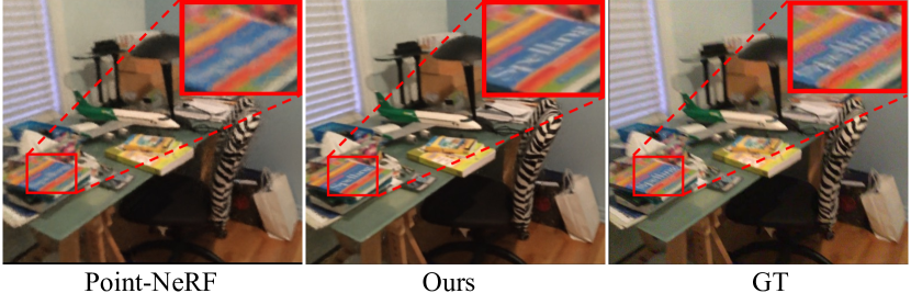
Figure 1: Our hybrid neural rendering model generates high-fidelity novel view images. Please note characters in the book where the result of Point-Nerf is blurry and the GT is contaminated by blur artifacts.

To improve novel view synthesis, mainstream research can be mainly categorized into two lines. One line of methods directly resorts to features from training data to synthesize novel view images  [31, 42, 5, 12], namely image-based rendering. By directly leveraging rich high-quality features from neighboring high-resolution images, these methods have a better chance of generating high-fidelity images with distinctive details. Nevertheless, the generated images often lack consistency due to the absence of global structural regularization, and boundary image pixels often contain serious artifacts. Another line of work attempts to equip NeRF with explicit 3D representations in the form of point cloud [45, 30], surface mesh [46, 32] or voxel grid features [21, 10, 48], namely neural 3D representation. Thanks to the global geometric regularization from explicit 3D representations, they can efficiently synthesize consistent novel view images but yet struggle with producing high-fidelity images in large-scale scenes (see the blurry images from Point-NeRF [45] in Fig. 1). This may be caused by low-resolution 3D representations [21], noisy geometries [1, 8], imperfect camera calibrations [2], or inaccurate rendering formulas [3], which make encoding a large-scale scene into a global neural 3D representation non-trivial and inevitably loses high-frequency information.

Albeit advancing the field, the above work all suffer immediately from low-quality training data, e.g., blurry images. Recently, Deblur-NeRF [23] aims to address the problem of blurry training data and proposed a pipeline to simulate blurs by querying multiple auxiliary rays, which, however, is computation and memory inefficient, hindering their applicability in large-scale scenes.

In this paper, we aim at synthesizing high-fidelity and view-consistent novel view images in large-scale scenes using in-the-wild unsatisfactory data, e.g., blurry data. First, to simultaneously address high fidelity and view consistency, we put forward a hybrid neural rendering approach that enjoys the merits of both image-based representation and neural 3D representation. Our fundamental design centers around a 3D-guided neural feature fusion module, which employs view-consistent neural 3D features to integrate high-fidelity 2D image features, resulting in a hybrid feature representation that preserves view consistency whilst simultaneously upholding quality. Besides, to avoid the optimization of the hybrid representation being biased toward one modality, we develop a random feature drop strategy to ensure that features from different modalities can all be well optimized.

Second, to effectively train the hybrid model with unsatisfactory in-the-wild data, we design a blur simulation and detection approach to alleviate the negative impact of low-quality data on model training. Specifically, the blur simulation module injects blur into the rendered image to mimic the real-world blurry effects. In this way, the blurred image can be directly compared with the blurry reference image while providing blur-free supervisory signals to train the hybrid model. Besides, to further alleviate the influence of blurry images, we design a content-aware blur detection approach to robustly assess the blurriness scores of images. The calculated scores are further used to adjust the importance of samples during training. In our study, we primarily focus on the blur artifact due to its prevalence in real-world data (e.g., ScanNet); however, our “simulate-and-detect” approach can also be applied to address other artifacts.

While our model is built upon the state-of-the-art 3D- and image-based neural rendering models, our contribution falls mainly on studying their combinatorial benefits and bridging the gap between NeRF and unsatisfactory data captured in the wild. Our major contributions can be summarized as follows.

• We study a hybrid neural rendering model for synthesizing high-fidelity and consistent novel view images.

• We design efficient blur simulation and detection strategies that facilitate offering blur-free training signals for optimizing the hybrid rendering model.

• Extensive experiments on real (i.e., ScanNet [6]) and synthetic data (i.e., Habitat-sim [24, 37]) showcase that our method outperforms state-of-the-art point-based methods designed for novel view synthesis.

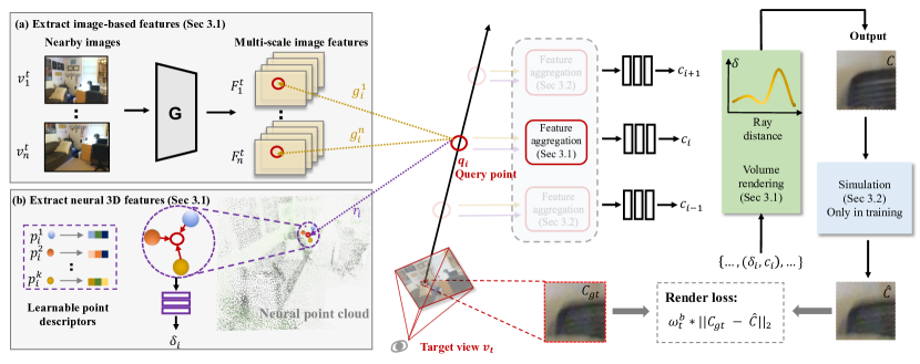
Figure 2: An overview of our hybrid neural rendering model $\mathcal{H}$. For each query point $q_{i}$ on a ray cast from the target view $v_{t}$, it has two modalities of features, i.e., (a) the image-based features $\{g_{i}^{1},...,g_{i}^{n}\}$ extracted from the $n$ nearby images $\{v_{1}^{t},...,v_{n}^{t}\}$ and (b) the neural 3D feature $r_{i}$ interpolated from $k$ neighboring point descriptors $\{p_{i}^{1},...,p_{i}^{k}\}$. To generate high-quality and consistent novel view images, our hybrid neural rendering aggregates and benefits from both features from two modalities. To handle blur artifacts in the reference images, we simulate blur effects on the rendered image patch $C$ to obtain $\hat{C}$, and then calculate the rendering loss with the ground-truth image patch $C_{gt}$. During training, we also down-weight the importance of images contaminated by artifacts according to the pre-computed quality-aware weights $\omega_{t}^{b}$ (see Sec. 3.2).

2 Related Works

Neural Radiance Field NeRF [25] encodes the object or scene into an MLP and synthesizes novel view images through volume rendering [16]. Later works extend NeRF for object manipulation [46, 47, 52, 15] and dynamic scene modeling [27, 28, 20], etc. Recent work [53, 45, 21] has started incorporating explicit 3D representations into NeRF training to support large-scale scenes and improve rendering details and speed. For example, Liu et al. [21] enhance NeRF’s capabilities by storing neural features in a voxel-based representation, which generates images with rich details. Similarly, Xu et al. [45] utilize a point-based neural radiance field in cooperation with point growing and pruning, which substantially speeds up training and improves the quality of the rendered image. Unlike the methods described above, we deliver a hybrid framework leveraging the advantages of neural 3D representation and image-based representation to yield high-quality images.

Image-Based Rendering Image-based rendering is a well-known and long-standing technique [19, 9] for generating novel view images. A typical pipeline is to identify a few nearby images, warp them to the target viewpoint, and then blend them to create the output [31, 12, 13]. Recently, image-based rendering methods collaborating with volume rendering have been developed for generalization across scenes [5, 42, 49]. For instance, IBRNet [42] employs extracted image features from neighboring images to directly predict target views without requiring per-scene optimization [25]. Since image-based rendering can directly use the rich textures from images, it typically converges faster. However, it generally suffers from temporal inconsistencies. Instead, we apply the globally consistent neural 3D feature to drive the blending process in this work, improving the consistency of rendered image sequences.

Rendering with Artifacts For the in-the-wild environments, it is almost impossible to capture artifact-free training data due to motion blurs, noise, and environmental factors, which can adversely affect rendering quality. One solution is to restore contaminated images first [40, 44, 35, 36, 7, 50, 43], and then use restored images for training. However, it is a challenging problem to maintain the view consistency of restored images [14] as a pre-trained network is used to process each frame independently. Recently, some works [11, 33, 23] have attempted to simulate the image degradation process for image restoration during training. For example, to remove reflections, Guo et al. [11] propose incorporating an auxiliary MLP to model the reflection effects, which is removed during inference. Rückert et al. [33] propose to learn exposure-related parameters and response functions for synthesizing HDR images from training images with various exposures. The work most related to us is Deblur-NeRF [23], which uses auxiliary rays to simulate blurs for each training image which, however, sacrifices computation efficiency. Instead of sampling extra rays, we propose to down-weight the importance of blurry images and design a simple and efficient blur simulation method, resulting in faster training and better results.

3 Method

Given RGB-D image sequences with inevitable in-the-wild artifacts, our approach aims to render high-quality and consistent novel view images. In our study, we consider motion blur as the major artifact due to its ubiquity in data captured with hand-held devices. An overview of our model is shown in Fig. 2. First, we put forward a hybrid neural rendering model $\mathcal{H}$ that incorporates neural features extracted from images and a geometry-aware neural radiance field (e.g., Point-NeRF) for producing high-quality and view-consistent synthesis results (see Sec. 3.1). Then, to produce blur-free supervisory signals for training the hybrid model, we develop a blur simulation module and a content-aware blur detection strategy to alleviate the negative impacts of blurry ground-truth reference images (see Sec. 3.2). At last, we introduce the loss functions and optimization strategies for training our models (see Sec. 3.3).

3.1 Hybrid Neural Rendering Model

Our hybrid neural rendering model is designed to combine image-based representation and the geometry-based neural radiance field for faithful and view-consistent synthesis. It consists of a neural feature extraction module to harvest information from two kinds of representations, and a neural feature fusion module to aggregate extracted neural features in a data-driven manner. Given the aggregated features, our approach renders output images based on volume rendering. During training, we design a random drop strategy to avoid the optimization being dominated by one of the two representations.

Neural Feature Extraction As shown in Fig. 2, for each query point $q_{i}$ on a ray cast from a target view $v_{t}$, we extract two modalities of features – image-based features and neural 3D features, described as follows.

Image-based features (Fig. 2 (a)): First, we use a lightweight CNN with down-sampling layers to extract multiscale image features $\{F_{1}^{t},F_{2}^{t},...,F_{n}^{t}\}$ from $n$ nearby views $\{v_{1}^{t},v_{2}^{t},....,v_{n}^{t}\}$. Then, the query point $q_{i}$ is projected to these nearby views, and features $\{F_{1}^{t}(q_{i}),F_{2}^{t}(q_{i}),...,F_{n}^{t}(q_{i})\}$ at the projected point location will be used to construct the image-based features for rendering. Following IBRNet [42], we additionally add image color $v_{j}^{t}(q_{i})$ and deviations of view directions $\Delta d_{j}^{t}(q_{i})$ to image-based features. As a result, for each query point $q_{i}$, its image-based feature representation is $g_{i}=\{g_{i}^{1},g_{i}^{2},...,g_{i}^{n}\}$ where $g_{i}^{j}$ is the combination of $F_{j}^{t}(q_{i})$, $v_{j}^{t}(q_{i})$, and $\Delta d_{j}^{t}(q_{i})$.

Neural 3D features (Fig. 2 (b)): We adopt a point-based neural 3D representation [45, 8, 1] due to the wide application and high availability of point clouds. Following Point-NeRF [45], we aggregate features from multi-view depth maps to obtain point-based 3D representations, i.e. each point is described by a learnable descriptor. Then the neural 3D feature $r_{i}$ is obtained by interpolating descriptors from its $k$-nearest neighborhoods $\{p_{i}^{1},p_{i}^{2},...,p_{i}^{k}\}$. Note that the point-based representation can be replaced with other geometry-based representations, such as voxel-based or mesh-based representations [21, 46].

Neural Feature Aggregation

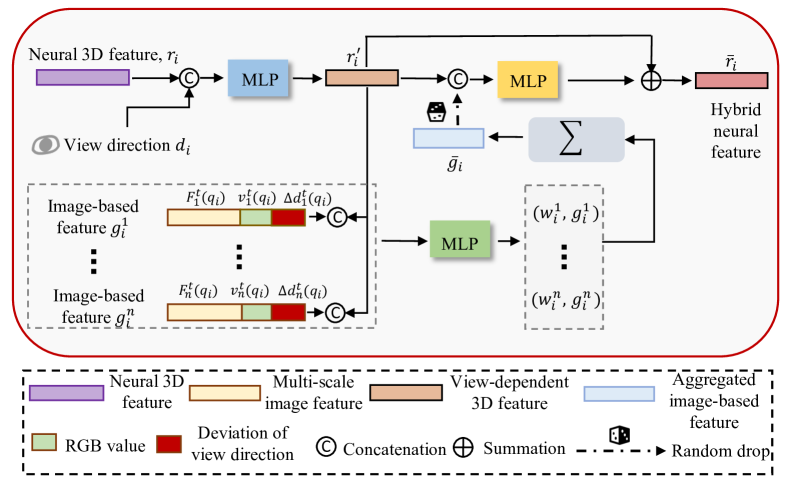
Figure 3: An overview of our feature aggregation module. The neural 3D feature $r_{i}$ and multiple image-based features $g_{i}^{n}$ are aggregated to generate a hybrid neural feature $\hat{r}_{i}$.

As shown in Fig. 3, given image-based features $g_{i}$ from $n$ nearby views and neural 3D features $r_{i}$, we design a learnable method to aggregate them to form a hybrid feature $\overline{r}_{i}$ for each query point $q_{i}$,

First, the neural 3D feature $r_{i}$ combined with the view direction $d_{i}$ is fed into an MLP to produce a view-dependent neural 3D feature $r^{\prime}_{i}=\text{MLP}(r_{i},d_{i})$. Then, as the neural 3D feature consistently maintains global information and is free from view occlusions, we use it together with the image-based features to generate aggregation weights $\{\omega_{i}^{1},\omega_{i}^{2},...\omega_{i}^{n}\}$ via an MLP layer (i.e., $\omega_{i}^{j}=\text{MLP}(r^{\prime}_{i},g_{i}^{j})$). Further, the aggregation weights are used to combine $\{g_{i}^{1},g_{i}^{2},...,g_{i}^{n}\}$ to form an aggregated image feature $\overline{g}_{i}$ following Eq. (1):

$$\overline{g}_{i}=\sum_{j=1}^{n}(\frac{\omega_{i}^{j}}{\gamma_{i}}\times g_{i}^{j}),~{}\text{where}~{}\gamma_{i}=\sum_{j=1}^{n}\omega_{i}^{j}.$$ (1)

Finally, we learn a residual term for $r^{\prime}_{i}$ to get the final hybrid neural feature $\overline{r}_{i}$. This is achieved by enhancing the neural 3D feature $r^{\prime}_{i}$ using the aggregated image features $\overline{g}_{i}$, which can be described as:

$$\overline{r}_{i}=r^{\prime}_{i}+\text{MLP}(r^{\prime}_{i},\overline{g}_{i}).$$ (2)

Volume Rendering As illustrated in Fig. 2, we use $k$ nearby geometric-consistent point descriptors $\{p_{i}^{1},p_{i}^{2},...,p_{i}^{k}\}$ to predict volume density $\delta_{i}$ considering the view-independent nature of 3D geometry. The radiance values $c_{i}$ are estimated through our hybrid neural features $\overline{r}_{i}$, which contain rich details. Then, we apply the volume rendering [25] to get the output color $c$ of each ray following Eq. 3:

$$c= \sum_{i=1}^{M}\tau_{i}(1-\text{exp}(-\delta_{i}\Delta_{i}))c_{i},$$ (3)

$$\tau_{i}=\text{exp}(-\sum_{t=1}^{i-1}\delta_{t}\Delta_{t}).$$

Here, M indicates the number of query points on a ray; $\Delta_{i}$ represents the distance between two adjacent query points along the ray, and the $\tau_{i}$ means volume transmittance.

Random Drop We develop two random drop strategies that randomly drop image features during optimization to ensure both modalities of features can be well-optimized: 1) the ray-based random drop will drop all image features on randomly selected rays; 2) the query-point-based random drop will randomly select query points on all rays and then remove all image features on them. The motivation behind the random drop is that we find the optimization of the hybrid representation can be easily dominated by image features, leaving neural 3D features poorly trained. This is because the image features are very similar to the reference images and are thus more easily optimized. Unless otherwise specified, we adopt the ray-based random drop during training. In the experiment part (see Fig. 10), we show the effects of the two strategies.

3.2 Blur Simulation and Detection

We propose two complementary strategies to address the negative influence of blurry reference images on optimizing the hybrid neural rendering model. First, we design a simulation method that simulates blur effects on the rendered image patch $C$ to imitate the blur effects of the reference image patch $C_{\text{gt}}$. By comparing the blurred image patch $\hat{C}$ with the reference image patch during training, the sharpness of the rendered images can be preserved. Second, we develop a content-aware detection method to pre-compute the blurriness scores of reference images and down-weight the importance of blurry images based on the calculated scores. The two strategies work collectively to address the data quality challenge.

Blur Simulation

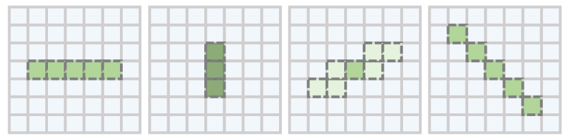
Figure 4: Examples of blur kernels. The pre-defined blur kernels have different moving directions and distances.

To simulate motion blur, we assume that the camera moves in one direction through a certain distance while capturing high frame rate videos. Specifically, we take into account $N_{v}$ directions and $N_{d}$ distances for creating blur kernels ($B_{i}|i=0,1,...,N_{v}\times N_{d}$) that are used to simulate blurs, and some examples of blur kernels are shown in Fig. 4. When $i=0$, it means no blur simulation. To determine which blur kernel approximates the blur effects best, we first apply all blur kernels to the rendered results to obtain the blurred image patches $\hat{C}_{i}=\text{Conv}(C,B_{i})$, and then choose the blur kernel $i$ that yields an output patch $\hat{C}_{i}$ with the minimum photo-metric loss w.r.t the reference image patch $C_{\text{gt}}$. This process is described as:

$$L_{i}=||\hat{C}_{i}-C_{\text{gt}}||_{2},$$ (4)

$$\mathcal{L}_{\text{color}}= \min\{L_{i}|i=0,1,...,N_{v}\times N_{d}\}.$$

Because our blur simulation does not need to render extra rays nor exhaustively optimize per-view embeddings as in Deblur-NeRF [23], it runs faster and is more memory efficient, making it suitable for large-scale scenes with dense views. This blur simulation process is removed during inference to produce sharp images $C$. (In appendix 6, we further propose a novel learnable scheme to efficiently predict degradation kernels by exploring differences between rendered and reference patches.)

Content-Aware Blur Detection In addition, we also down-weight the contribution of blurry images based on the blurriness score (a smaller value indicates more severe blur artifacts). However, we find that the “variation of the Laplacian” [29] method used to compute blurriness scores is prone to be influenced by image contents, thus unsuitable for scoring the reference images directly. As shown in the left of Fig. 5, the upper image is sharper than the bottom one but has a lower blurriness score. This is because the upper image contains more textureless contents (i.e., the floor).

To exclude the influence of image contents, we develop a content-aware blur detection approach, which outputs accurate blurriness scores by scoring the overlapping regions. As shown in Fig. 5 right, our method first takes two neighboring images $\{I_{t},I_{t+1}\}$ as inputs and estimates their overlapping regions (blue areas in Fig. 5) using optical flow [39]. Then, it returns two images’ blurriness scores $\{S_{t}^{1},S_{t+1}^{1}\}$ calculated from the overlapping regions. Next, to compute the blurriness score of image $I_{t+2}$, we use another image pair $\{I_{t+1},I_{t+2}\}$ and repeat the process above to obtain two new blurriness scores $\{S_{t+1}^{2},S_{t+2}^{1}\}$. Considering different overlapping regions in an image (e.g., blue and red regions of $I_{t+1}$ in Fig. 5) will lead to different blurriness scores $S_{t+1}^{1}$ and $S_{t+1}^{2}$, we align them by scaling $S_{t+1}^{2}$ to $S_{t+1}^{1}$. Correspondingly, the blurriness score of $I_{t+2}$ is scaled following $S_{t+2}^{1}=S_{t+1}^{1}/S_{t+1}^{2}\times S_{t+2}^{1}$. Similarly, the blurriness scores of other images can be computed. Please refer to the supplementary file for details. Finally, we convert blurriness scores into quality-aware weights $\omega_{t}^{b}$ following:

$$\omega_{t}^{b}=(\frac{N\times S_{t}^{1}}{\sum_{t=0}^{N}S_{t}^{1}})^{\alpha},$$ (5)

where $N$ represents the number of images, and $\alpha\geq 0$ is a hyper-parameter used to adjust the distribution of quality-aware image weights. These weights are further applied to the training objective in Sec. 3.3 to down-weight the importance of blurry images. Alternatively, you can use $\omega_{t}^{b}$ as sampling probabilities to sample training images.

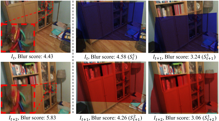
Figure 5: Content-aware blur detection. Left: the blurriness score [29] (large is sharper) is highly affected by image contents, and is usually low when the image contains textureless contents (e.g., floor). Right: the content-aware blur detection computes blurriness scores on overlapping regions of two images, thus obtaining more accurate scores.

3.3 Optimization

Our training objective consists of a photometric loss $\mathcal{L}_{\text{color}}$ in Eq. (4) that requires the rendered image patch $C$ after blur simulation $\hat{C}$ to have the same appearance as the reference image patch $C_{\text{gt}}$; and a sparsity loss $\mathcal{L}_{\text{sparse}}$ [22, 45] that encourages each point to have a confidence of 0 or 1 for the follow-up point pruning and growing operations. Following Point-NeRF [45], the point growing and pruning operations are applied every 10k iterations. After incorporating the quality-aware design ($\omega_{t}^{b}$ in Sec. 3.2), the final training objective is defined as:

$$\mathcal{L}_{t}=\omega_{t}^{b}(\mathcal{L}_{\text{color}}+\beta\mathcal{L}_{\text{sparse}}),$$ (6)

where $\beta=0.002$ is used to balance different loss terms and $\omega_{t}^{b}$ is the estimated blurriness score to down weight blurry images (see Section 3.2).

4 Experiments

4.1 Implementation Details

Network and Training The 2D CNN ($G$) used to extract image features has three down-sampling layers, and the point-based neural 3D representation is constructed following Point-NeRF [6]. We select four neighboring frames ($n=4$) and eight nearest point descriptors ($k=8$) to extract neural features. We train our models using the Adam [17] optimizer with an initial learning rate of $0.0005$. A total of 200k iterations are used for training.

Blur Simulation We build our blur kernels considering $N_{v}=4+8$ directions (i.e., ‘left-right’, ‘up-down’, ‘top left-bottom down’, and ‘bottom left-top right’; both symmetrical and asymmetrical) and three moving distances $N_{d}=3$ (i.e., 1, 2, 4). To apply blur simulation, we sample $8\times 8$ patches with dilations [34] during the training, and the $\alpha$ in Eq. (5) is set as 1.

Dataset We conduct our experiments on ScanNet [6] and synthetic data generated from Habitat-sim [24]. 1) ScanNet [6] contains RGB-D image sequences captured in large-scale indoor scenes with handheld sensors. Following Point-NeRF, we conduct experiments on “Scene0101_04” and “Scene0241_01” and select every fifth image for training and the remaining images for testing. Note that images in the ScanNet are blurry, which is not suitable for quantitatively evaluating the sharpness of rendered images. Thus, we additionally evaluate our method using synthetic data. 2) Habitat-sim is a simulator [24, 38] that synthesizes blur-free RGB-D sequences of large-scale scenes (i.e., ’VangoRoom’ and ’LivingRoom’ [37]). We then add motion blurs to the synthesized training sets. Please see the supplementary file for details.

Baselines We compare our method with other representative image-based and neural-radiance-based novel view synthesis approaches, including: 1) NeRF [25]; 2) IBRNet [42] which combines image-based rendering with volume rendering and generates high-quality novel view images without using depth; 3) NPBG [1] which renders images using a U-Net-like design by rasterizing point descriptors onto the image plane 4) Point-NeRF [45], which is the state-of-the-art point-based method for novel view synthesis combining point-based neural representation and neural radiance field with volume rendering; and 5) Deblur-NeRF [23] which improves the sharpness of rendered images by simulating the blurring process with a deformable sparse kernel module.

4.2 Results on ScanNet

Quantitative comparisons with other baselines in terms of PSNR, SSIM, and LPIPS [51] are reported in Table 1. Our hybrid neural rendering design “Ours (H)” outperforms previous methods by enhancing the quality of neural 3D representations. However, the PSNR and SSIM drop in the full version of our method “Ours”. This is because our blur-handling modules mimic blurriness effects and down weight blur images, enabling the model to learn from clean supervision. However, since this differs from the original training data distribution, the model may not fit the evaluation metric well. Moreover, Deblur-NeRF delivers a low PSNR because it tends to introduce misalignment between rendered and reference images.

We show qualitative comparisons in Fig. 6. Our method can render high-quality novel view images while other baselines suffer severely from blurriness and distortions. For example, the clock on the wall is distorted with IBRNet, and the book generated by Point-NeRF is blurry. In contrast, our model produces results with clear characters in the book (Fig. 6 “Ours (H)”), validating the efficacy of our hybrid representation. Further, the rendered images become sharper when using our design to handle blur artifacts; please notice the human face on the poster (Fig. 6 “Ours”). To better demonstrate the efficacy of our approach in rendering consistent results, we provide videos in the supplementary file: our results are more temporally consistent than the image-based rendering (i.e., IBRNet), thanks to the globally consistent neural 3D features.

	Scene101_04			Scene241_01
	PSNR$\uparrow$	SSIM$\uparrow$	LPIPS$\downarrow$	PSNR$\uparrow$	SSIM$\uparrow$	LPIPS$\downarrow$
Point-NeRF [45]	29.88	0.913	0.203	30.54	0.910	0.236
IBRNet [42]	29.55	0.811	0.307	21.49	0.755	0.368
NPBG [1]	26.33	0.871	0.187	27.34	0.841	0.188
Deblur-NeRF [23]	24.55	0.693	0.308	20.66	0.652	0.401
NeRF [25]	27.16	0.730	0.350	21.69	0.610	0.494
Ours (H)	30.33	0.919	0.186	31.25	0.918	0.218
Ours	29.33	0.909	0.181	30.78	0.914	0.206

Table 1: Quantitative comparisons on ScanNet. “Ours (H)”: use hybrid neural rendering without handling blur artifacts. We use PSNR, SSIM, and LPIPS to evaluate the rendering quality ($\downarrow$: small is better; $\uparrow$: large is better). Our method outperforms all other baselines by a large margin, especially on PSNR. Note that the full version of our method (“Ours”) is worse on the PSNR and SSIM, this is because the reference images in ScanNet are blurry.

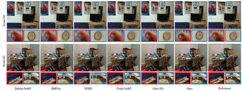
Figure 6: Qualitative comparisons on ScanNet. The highlighted regions are zoomed-in and placed at the bottom for better comparisons. From the results, our method can synthesize sharper images than other approaches that are suffering from blurriness, distortions, and jagged edges. Moreover, the sharpness is further improved after applying our design to handle blur artifacts (i.e., Ours vs. Ours (H)).

4.3 Results on Synthetic Data

We conduct experiments on the synthetic data to validate our designs to handle blurriness. In particular, we incorporate our designs into two different frameworks (i.e., NeRF and Point-NeRF) to show its generalization ability. Here, we remove the image-based rendering branch on the NeRF-based framework for fair comparisons. Fig. 7 shows that our method significantly enhances the sharpness of rendered images compared to NeRF and Point-NeRF, which are also confirmed in Table 2. Notably, images from Deblur-NeRF contain more details than NeRF but suffer from distorted image structures, such as the blinds and the table leg. This is possible because the learning of ray deformation is under-constrained with too many degrees of freedom and thus prone to corrupting original structures, or the view embeddings are not well-optimized due to the increased number of training views. Our easy-to-plug-in method outperforms Deblur-NeRF on PSNR and SSIM and delivers competitive performance on LPIPS. It is worth noting that to achieve the above results, NeRF takes 4.5 hours, while our method takes 4.6 hours. Thus, the increase in training time brought by blur simulation is negligible. However, Deblur-NeRF needs 8.5 hours which incurs much more overheads. The time is reported with training the model on a single NVIDIA 3090 GPU.

	VangoRoom			LivingRoom
	PSNR$\uparrow$	SSIM$\uparrow$	LPIPS$\downarrow$	PSNR$\uparrow$	SSIM$\uparrow$	LPIPS$\downarrow$
NeRF	28.83	0.769	0.339	29.73	0.848	0.215
Deblur-NeRF [23]	29.30	0.793	0.247	31.82	0.895	0.132
Ours+NeRF	30.26	0.805	0.259	32.70	0.912	0.124
Point-NeRF	31.24	0.950	0.152	32.20	0.959	0.109
Ours+Point-NeRF	33.27	0.966	0.097	35.30	0.980	0.051

Table 2: Quantitative comparisons on the synthetic data. We apply our design used to handle blur artifacts to two different frameworks, i.e., NeRF and Point-NeRF. With our design, the values of all three metrics receive significant improvements.

Figure 7: Qualitative comparisons on the synthetic data. We validate our designs to deal with blur artifacts on two different frameworks, i.e., NeRF and Point-NeRF. By applying our design, the details of rendered images become sharper. Besides, the Deblur-NeRF can also improve the sharpness, but the structure (e.g., blinds) is distorted.

4.4 Ablation Studies

In this section, we conduct comprehensive ablations of the proposed designs in our method.

Advantages of Image Features We first assess the contribution of image features in our system by comparing “Ours (H)” and Point-NeRF (i.e., without using image features). As shown in Fig. 6 and Table 1, our method benefits from image features and outperforms Point-NeRF. Moreover, our hybrid model converges faster. For example, we achieve PSNR 31.0 after 20k iterations (80 minutes) on “Scene241$\_$01”, whereas Point-NeRF delivers 29.3 PSNR after 40k iterations (84 minutes). (Please refer to supplementary material for more results.) This is because compressing all information into a neural 3D representation is difficult since it requires accurate camera poses, high-resolution 3D representations, etc. On the contrary, high-fidelity image features can directly compensate for defective neural 3D features and enable synthesizing high-quality results with fewer training iterations.

Advantages of Neural 3D Features We then show the value of the neural 3D feature by comparing it with IBRNet, which uses only image features. From the results in Fig. 6 and the video in the supplementary material, the rendered images from IBRNet are often distorted and inconsistent due to the lack of global 3D constraints. To further investigate the efficacy of learned neural 3D representations, we replace the neural 3D features with the mean and variance of image features extracted from nearby frames in the feature aggregation module (see Fig. 3). The corresponding results are displayed in Fig. 8, our approach preserves the shape consistency of the chair leg.

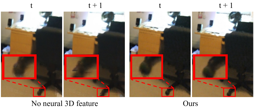
Figure 8: Advantages of neural 3D features. Without using the neural 3D feature, the rendered images will be inconsistent at different times. This can be observed in the example of the chair leg.

Blur Simulation and Quality-aware Design We further show the effect of blur simulation and detection by removing each of them at a time, and the results on “LivingRoom” are shown in Table 3. According to Table 3, both components contribute to the final performance, and the performance is improved when they are combined.

	NeRF-Based			Point-NeRF-Based
	PSNR$\uparrow$	SSIM$\uparrow$	LPIPS$\downarrow$	PSNR$\uparrow$	SSIM$\uparrow$	LPIPS$\downarrow$
Baseline	29.73	0.848	0.215	32.20	0.959	0.109
+ Blur simulation	32.24	0.905	0.133	34.32	0.974	0.065
+ Quality-aware weight	31.81	0.900	0.148	34.48	0.977	0.065
Full	32.70	0.912	0.124	35.30	0.980	0.051

Table 3: We validate our designs to handle blur artifacts on the ’LivingRoom’. Each component improves the performance and works better when combined.

Random Drop Methods The random drop strategy is to avoid the optimization being dominated by image features. As shown in Fig. 9, without using random drop in the training process, the results are poor in areas not covered by image features (the right side of the sofa). This region can only rely on neural 3D representation for rendering; thus, the poor results imply that the neural 3D representations are not well optimized. In contrast, our method with the random drop strategy produces high-quality images. Moreover, we observe that the results are slightly different when using different variants of the random drop strategy. For example, the rendered image is automatically enhanced using query-point-based random drop, as displayed in Fig. 10. One possible explanation is that, during training, the use of volume rendering for aggregation automatically enhances query points with image features to compensate for query points with low-quality neural 3D features on the same ray. However, this enhancement tends to change the color tone, as demonstrated in the bicycle example in Fig. 10. Thus, we currently adopt the ray-based random drop to render images having a closer appearance to the reference images.

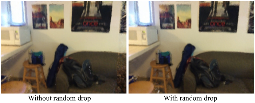
Figure 9: Efficacy of random drop. Without random drop, areas around image boundary (e.g., the sofa in the left image) not covered by image features are bad.

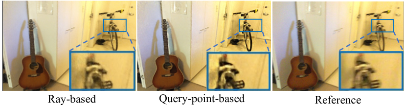
Figure 10: Different random drop methods. Query-point-based random drop automatically enhances the rendered images, but it tends to change the color tone. Please note the bicycle.

5 Conclusion

In this paper, we present an approach to render high-fidelity and view-consistent images in large-scale scenes from sources contaminated by motion blurs. We develop a hybrid neural rendering model that makes use advantages of both image-based representation and neural 3D representation to render high-quality and view-consistent results. We also propose to efficiently simulate blur effects on the rendered image and design a quality-aware training strategy to down-weight blurry images, which helps the hybrid neural rendering model learn from blur-free supervisions and generate high-fidelity images. We conduct experiments on both real and synthetic data and obtain superior performance over previous methods.

Limitations Our method focuses on dealing with simple motion blurs in the training data, and defocus blur is not considered. Moreover, there are many other in-the-wild challenges, such as images captured under different exposure times and light conditions that require further research.

Acknowledgement This work has been supported by Hong Kong Research Grant Council - Early Career Scheme (Grant No. 27209621), General Research Fund Scheme (Grant no. 17202422), and RGC matching fund scheme.

Appendix

Overview This document begins by introducing an extendable scheme for predicting the degradation kernel in Section 6. We then present additional implementation details on network structures, the generation process of synthetic data, and content-aware blur detection in Section 7. At last, we investigate model capacity in Section 8 before conducting additional experiments and presenting more results on challenging scenarios and diverse datasets in Section 9.

6 Learnable Degradation Kernel

Method By comparing the appearance of rendered and reference patches, it is possible to predict the potential degradation kernel $B_{\text{final}}$ that makes up for their difference. To comprehensively explore the patches and efficiently predict the degradation kernel, we adopt a shallow MLP here. More specifically, the rendered and reference patches are first grayscaled and flattened, and then they are concatenated and fed into an MLP to predict a kernel $B_{p}$ and a blending weight $\omega_{p}$. At last, the degradation kernel $B_{\text{final}}$ is obtained by blending the predicted kernel $B_{p}$ and the identity kernel $B_{I}$ consisting of zeros except for the center point, which is set as one:

$${B}_{final}=\omega_{p}*B_{p}+(1-\omega_{p})*B_{I}.$$ (7)

After this, we can directly apply the final degradation kernel to the rendered patch to avoid the negative influence of defective training data (see Fig. 11).

More discussions 1) To handle view-dependent inconsistencies, previous methods need to optimize a latent code for each training view, and the training time is proportional to the number of training views since each view must be exhaustively sampled to well optimize the corresponding latent code. In contrast, our method directly studies generalizable cues in image patches or uses predefined kernels, and thus is less limited by the number of training views, especially in large-scale scenes covered by dense views. In the future, how to integrate image cues and the per-view latent code optimization is worth exploring. 2) Even though our method focuses on per-scene optimization, the patch/image-based design would enjoy the benefits of pre-training [42, 49]. 3) The learnable degradation kernel is very flexible and thus may not be limited to blur artifacts. For example, we can try to use the rendered and reference patches to predict the alignment kernel, where each position represents a motion vector to account for misalignments caused by rough geometries, incorrect camera calibrations, and image distortions.

Results We validate the effectiveness of learned degradation kernels by conducting experiments on the “LivingRoom” dataset using the point-based framework. When compared to the results of pre-defined degradation kernels, the learned degradation kernel achieves 0.5 improvements on PSNR, as shown in Table 4. As for efficiency, it takes about 10 hours to train (200K iterations) when using only hybrid neural rendering, and an additional 0.5 hours to learn the degradation kernels.

LivingRoom	PSNR$\uparrow$	SSIM$\uparrow$	LPIPS$\downarrow$
Pre-defined kernels	35.30	0.980	0.051
Learned kernels	35.81	0.981	0.050

Table 4: Results of using different degradation kernels.

In Fig. 11 (a), we visualize the learned degradation kernel. When this kernel is applied to the rendered sharp image patch (Fig. 11 (b)), the resulting degraded image patch (Fig. 11 (c)) more closely resembles the blurry reference image patch (Fig. 11 (d)), allowing for the preservation of high-frequency information.

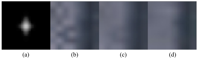
Figure 11: Visualization of learnable degradation kernel. (a) The predicted degradation kernel. (b) The rendered image patch. (c) Apply the degradation kernel to the rendered image patch. (d) The blurry reference image patch.

7 More Implementation Details

Network Architectures Our network consists of three major components. 1) The image feature extractor ($G$). It extracts multi-scale image features using $3\times 3$ kernels. We double the intermediate channels when down-sampling with a stride of 2. Totally, it has six layers with intermediate channels of {6, 6, 12, 12, 24, 24}. 2) MLPs in the feature aggregation. In Figure 3 of the main paper, the blue MLP consist of three layers with intermediate channels of {128, 128, 128}, and the green MLP has four layers with intermediate channels of {64, 64, 64, 1}, and the yellow MLP has three layers with intermediate channels of {45, 45, 45}. 3) MLPs for color and volume density prediction. In Figure 2 of the main paper, the purple MLP used to predict volume density has five layers with intermediate channels of {256, 256, 256, 256, 1}. Additionally, the black MLP that generates color from the hybrid feature has one layer with three output channels.

Synthetic Data The $480\times 640$ RGB-D image sequences synthesized from Habitat-sim [24, 38, 37] are sharp. Following the train and test split on ScanNet, we divide the entire dataset into training sets (every 5th image) and testing sets. We then simulate motion blurs [18] on the training sets (RGB images) to obtain blurry training images. Specifically, each image has a probability of 0.75 of being blurred using a motion blur simulator [18]. The simulator has two hyperparameters: size and intensity, which control the properties of the motion blur. The size parameter $k$ controls the moving distance, and is uniformly sampled from the range $k\in(3,16)$. The intensity parameter $\phi$ determines the level of shake in the moving direction. As we assume that the camera moves in one direction at a given moment while capturing high frame rate videos, we randomly choose a small intensity value of $\phi\in(0,0.1)$. Note that our model is trained using randomly sampled small patches; therefore, this blur simulation process operates appropriately on small patches.

Content-Aware Blur Detection To calculate the blurriness score, we use a method called “variation of the Laplacian” [29]. First, we apply a blur kernel (i.e., mean filter in our paper) to the original RGB image $I$ to reduce the influence of noise. Then, we use the Laplacian operator to extract the high-frequency components $\hat{H}$ from the denoised image $\hat{I}$. Finally, we obtain the blurriness score by computing the variation of all high-frequency components $S=var(\hat{H})$.

To prevent the inaccurate blurriness score of one frame from affecting the subsequent frames, we implement our content-aware detection (Sec. 3.2 in the main paper) using a sliding window scheme in practice. Specifically, the sliding window incorporates 10 frames (i.e., $N=10$) to calculate quality-aware weights $\omega_{i}^{b}$, and moves in steps of 5 on the time axis. If a frame is covered multiple times by the sliding window, the final quality-aware weight is the average of all weights belonging to that frame. In this paper, we use consecutive frames since videos are provided. Similarly, neighboring frames can also be used to compute overlapping regions in place of consecutive frames.

8 Model Capacity

To further confirm that the improvements of our method, which builds upon Point-NeRF, are not dependent on larger model capacities, we conducted two experiments on Point-NeRF: 1) Gradually increasing the number of points from 4.2 million to 7.4 million, and 2) Increasing the channels of each point descriptor from 32 to 63. Results in Table 5 indicate that naively increasing the capacity of Point-Nerf does not improve performance. Moreover, the total number of parameters optimized in Point-NeRF with 7.4 million points (model size: 1.2 GB) already exceeds that of our hybrid model with 4.2 million points (model size: 682 MB, PSNR: 31.25).

Number of points	4.2M	5.3M	6.3M	7.4M	4.2M
Number of channels	32	32	32	32	63
Point-NeRF (PSNR)	30.54	30.56	30.55	30.50	30.58

Table 5: Results on “Scene241_01” while increasing the number of point descriptors and channels of each descriptor. Naively increasing the capacity of Point-NeRF cannot boost performance.

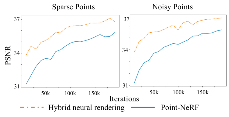
Figure 12: The trend of PSNR across different training iterations is shown for the case of sparse points and noisy points. When using image features (i.e., hybrid neural rendering), the performance is better than the neural-3D-feature-only design (i.e., Point-NeRF).

9 More Experiments

Sparse and Noisy Points We conduct experiments on challenging situations using sparse (0.6M points) and noisy (add gaussian noise $\mathcal{N}(0,0.05)$) points on ’VangoRoom’ (to validate the effectiveness of image features, all blur-related designs are disabled, and images used for training and testing are blur-free). As shown in Fig. 12, using image features converges faster and achieves better performance than Point-NeRF, which only utilizes neural 3D features.

ARKITScenes Dataset We present results on the ARKITScenes dataset (“Scene_40776204”) [4]. Fig. 13 demonstrates the effectiveness of our hybrid rendering and blur-handling designs, where all components contributing to the sharpness of rendered images (note the bird). Quantitative results in Table 6 indicate that our method outperforms Point-NeRF on all three metrics.

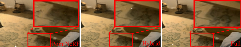
Figure 13: Qualitative results on the ARKITScenes dataset. Each component of our proposed method contributes to the sharpness of rendered images.

“Scene_40776204”	PSNR$\uparrow$	SSIM$\uparrow$	LPIPS$\downarrow$
Point-NeRF	31.02	0.947	0.212
Ours(H)	32.55	0.961	0.127
Ours(Full)	31.97	0.957	0.135

Table 6: Quantitative results on the ARKITScenes dataset.

NeRF Synthetic Dataset We provide results on the NeRF synthetic dataset (“Chair”) [25], which only provides posed RGB images without depth information. When trained for 66 minutes, our method leveraging image-based features produces results with more high-frequency details, as displayed in Fig. 14. This observation is also corroborated by quantitative results presented in Table 7.

ScanNet Dataset In Fig. 15, we show more qualitative results and compare them with Point-NeRF to demonstrate the superiority of our approach. We observed that the outputs of Point-NeRF suffer from blurry outputs and noisy edges, while “Ours (H)” contains more details and smoother appearance, evident in the toy plane in the third row and characters on the posters in the last two rows. Moreover, the image sharpness is further improved while applying our designs to handle blur artifacts.

Video Results In the video results, we compare our approach with other baselines, including NeRF [25], IBRNet [42], NPBG [1], Point-NeRF [45] and Deblur-NeRF [23], to demonstrate the superiority of our approach in terms of quality and consistency. Moreover, we also validate the effectiveness of our designs, including hybrid rendering, handling blurriness, random drop, and neural 3D features.

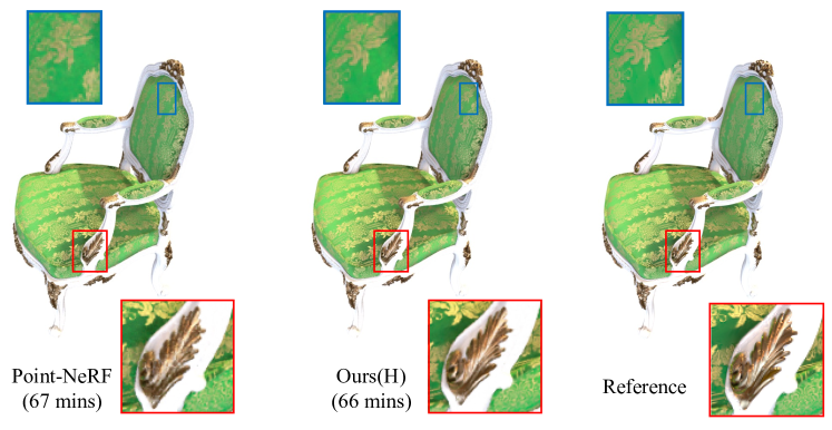
Figure 14: Qualitative results on the NeRF synthetic data. Leveraging image features assists in high-frequency details generation.

“Chair”	PSNR$\uparrow$	SSIM$\uparrow$	LPIPS$\downarrow$
$\text{Point-NeRF}_{40k}$ (67 mins)	33.80	0.986	0.017
$\text{Ours (H)}_{20k}$ (66 mins)	34.40	0.988	0.016
$\text{Point-NeRF}_{200k}$	35.70	0.992	0.010
$\text{Ours (H)}_{200k}$	36.23	0.993	0.009

Table 7: Quantitative results on the NeRF synthetic dataset. Our method outperforms Point-NeRF in both scenarios where training is performed for the same amount of time and the same number of iterations.

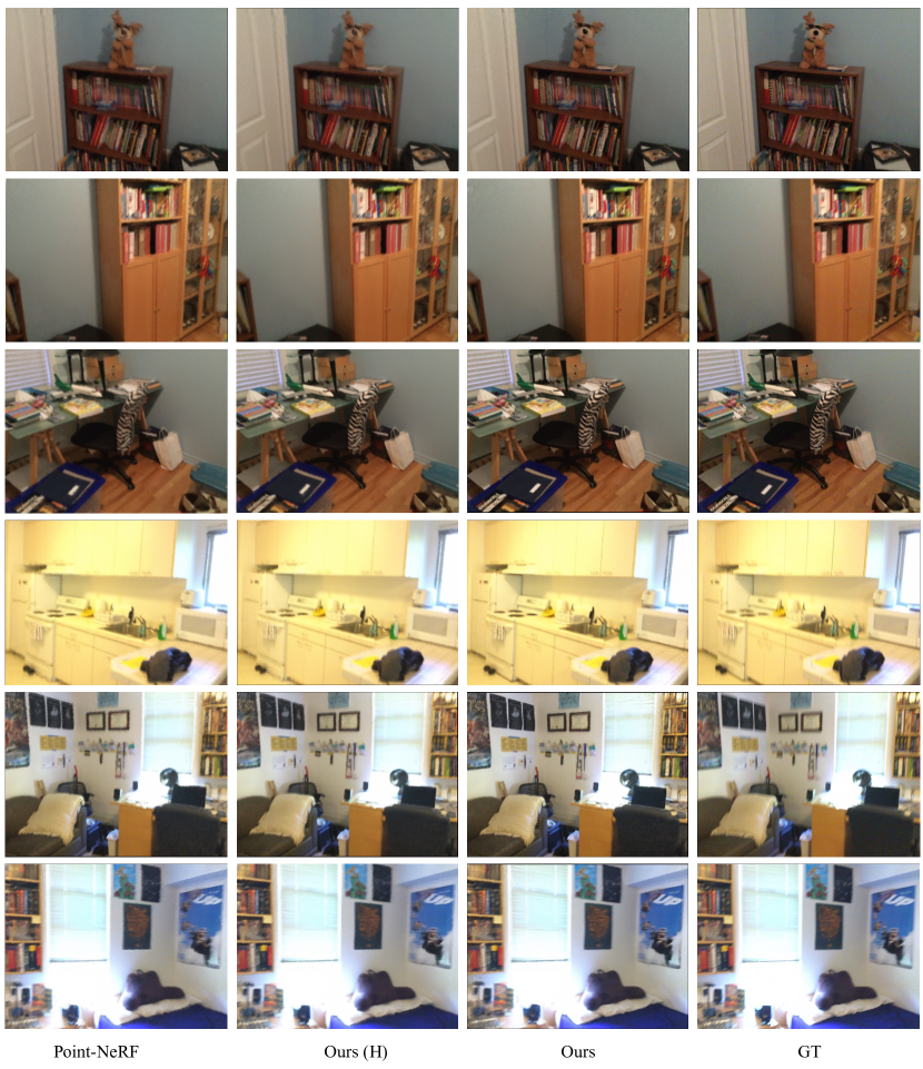
Figure 15: More results compared to Point-NeRF.

References

- [1] Kara-Ali Aliev, Artem Sevastopolsky, Maria Kolos, Dmitry Ulyanov, and Victor Lempitsky. Neural point-based graphics. In European Conference on Computer Vision, pages 696–712. Springer, 2020.
- [2] Dejan Azinović, Ricardo Martin-Brualla, Dan B Goldman, Matthias Nießner, and Justus Thies. Neural rgb-d surface reconstruction. In Proceedings of the IEEE/CVF Conference on Computer Vision and Pattern Recognition, pages 6290–6301, 2022.
- [3] Jonathan T Barron, Ben Mildenhall, Matthew Tancik, Peter Hedman, Ricardo Martin-Brualla, and Pratul P Srinivasan. Mip-nerf: A multiscale representation for anti-aliasing neural radiance fields. In Proceedings of the IEEE/CVF International Conference on Computer Vision, pages 5855–5864, 2021.
- [4] Gilad Baruch, Zhuoyuan Chen, Afshin Dehghan, Tal Dimry, Yuri Feigin, Peter Fu, Thomas Gebauer, Brandon Joffe, Daniel Kurz, Arik Schwartz, and Elad Shulman. ARKitscenes - a diverse real-world dataset for 3d indoor scene understanding using mobile RGB-d data. In Thirty-fifth Conference on Neural Information Processing Systems Datasets and Benchmarks Track (Round 1), 2021.
- [5] Anpei Chen, Zexiang Xu, Fuqiang Zhao, Xiaoshuai Zhang, Fanbo Xiang, Jingyi Yu, and Hao Su. Mvsnerf: Fast generalizable radiance field reconstruction from multi-view stereo. In Proceedings of the IEEE/CVF International Conference on Computer Vision, pages 14124–14133, 2021.
- [6] Angela Dai, Angel X Chang, Manolis Savva, Maciej Halber, Thomas Funkhouser, and Matthias Nießner. Scannet: Richly-annotated 3d reconstructions of indoor scenes. In Proceedings of the IEEE conference on computer vision and pattern recognition, pages 5828–5839, 2017.
- [7] Peng Dai, Xin Yu, Lan Ma, Baoheng Zhang, Jia Li, Wenbo Li, Jiajun Shen, and Xiaojuan Qi. Video demoireing with relation-based temporal consistency. In Proceedings of the IEEE/CVF Conference on Computer Vision and Pattern Recognition, pages 17622–17631, 2022.
- [8] Peng Dai, Yinda Zhang, Zhuwen Li, Shuaicheng Liu, and Bing Zeng. Neural point cloud rendering via multi-plane projection. In Proceedings of the IEEE/CVF Conference on Computer Vision and Pattern Recognition, pages 7830–7839, 2020.
- [9] Paul E Debevec, Camillo J Taylor, and Jitendra Malik. Modeling and rendering architecture from photographs: A hybrid geometry-and image-based approach. In Proceedings of the 23rd annual conference on Computer graphics and interactive techniques, pages 11–20, 1996.
- [10] Sara Fridovich-Keil, Alex Yu, Matthew Tancik, Qinhong Chen, Benjamin Recht, and Angjoo Kanazawa. Plenoxels: Radiance fields without neural networks. In Proceedings of the IEEE/CVF Conference on Computer Vision and Pattern Recognition, pages 5501–5510, 2022.
- [11] Yuan-Chen Guo, Di Kang, Linchao Bao, Yu He, and Song-Hai Zhang. Nerfren: Neural radiance fields with reflections. In Proceedings of the IEEE/CVF Conference on Computer Vision and Pattern Recognition, pages 18409–18418, 2022.
- [12] Peter Hedman, Julien Philip, True Price, Jan-Michael Frahm, George Drettakis, and Gabriel Brostow. Deep blending for free-viewpoint image-based rendering. ACM Transactions on Graphics (TOG), 37(6):1–15, 2018.
- [13] Peter Hedman, Tobias Ritschel, George Drettakis, and Gabriel Brostow. Scalable inside-out image-based rendering. ACM Transactions on Graphics (TOG), 35(6):1–11, 2016.
- [14] Yi-Hua Huang, Yue He, Yu-Jie Yuan, Yu-Kun Lai, and Lin Gao. Stylizednerf: consistent 3d scene stylization as stylized nerf via 2d-3d mutual learning. In Proceedings of the IEEE/CVF Conference on Computer Vision and Pattern Recognition, pages 18342–18352, 2022.
- [15] Wei Jiang, Kwang Moo Yi, Golnoosh Samei, Oncel Tuzel, and Anurag Ranjan. Neuman: Neural human radiance field from a single video. arXiv preprint arXiv:2203.12575, 2022.
- [16] James T Kajiya and Brian P Von Herzen. Ray tracing volume densities. ACM SIGGRAPH computer graphics, 18(3):165–174, 1984.
- [17] Diederik P Kingma and Jimmy Ba. Adam: A method for stochastic optimization. arXiv preprint arXiv:1412.6980, 2014.
- [18] LeviBorodenko. Motionblur, 2020. https://github.com/LeviBorodenko/motionblur.
- [19] Marc Levoy and Pat Hanrahan. Light field rendering. In Proceedings of the 23rd annual conference on Computer graphics and interactive techniques, pages 31–42, 1996.
- [20] Tianye Li, Mira Slavcheva, Michael Zollhoefer, Simon Green, Christoph Lassner, Changil Kim, Tanner Schmidt, Steven Lovegrove, Michael Goesele, Richard Newcombe, et al. Neural 3d video synthesis from multi-view video. In Proceedings of the IEEE/CVF Conference on Computer Vision and Pattern Recognition, pages 5521–5531, 2022.
- [21] Lingjie Liu, Jiatao Gu, Kyaw Zaw Lin, Tat-Seng Chua, and Christian Theobalt. Neural sparse voxel fields. Advances in Neural Information Processing Systems, 33:15651–15663, 2020.
- [22] Stephen Lombardi, Tomas Simon, Jason Saragih, Gabriel Schwartz, Andreas Lehrmann, and Yaser Sheikh. Neural volumes: Learning dynamic renderable volumes from images. arXiv preprint arXiv:1906.07751, 2019.
- [23] Li Ma, Xiaoyu Li, Jing Liao, Qi Zhang, Xuan Wang, Jue Wang, and Pedro V Sander. Deblur-nerf: Neural radiance fields from blurry images. In Proceedings of the IEEE/CVF Conference on Computer Vision and Pattern Recognition, pages 12861–12870, 2022.
- [24] Manolis Savva*, Abhishek Kadian*, Oleksandr Maksymets*, Yili Zhao, Erik Wijmans, Bhavana Jain, Julian Straub, Jia Liu, Vladlen Koltun, Jitendra Malik, Devi Parikh, and Dhruv Batra. Habitat: A Platform for Embodied AI Research. In Proceedings of the IEEE/CVF International Conference on Computer Vision (ICCV), 2019.
- [25] Ben Mildenhall, Pratul P Srinivasan, Matthew Tancik, Jonathan T Barron, Ravi Ramamoorthi, and Ren Ng. Nerf: Representing scenes as neural radiance fields for view synthesis. Communications of the ACM, 65(1):99–106, 2021.
- [26] Michael Niemeyer, Jonathan T Barron, Ben Mildenhall, Mehdi SM Sajjadi, Andreas Geiger, and Noha Radwan. Regnerf: Regularizing neural radiance fields for view synthesis from sparse inputs. In Proceedings of the IEEE/CVF Conference on Computer Vision and Pattern Recognition, pages 5480–5490, 2022.
- [27] Keunhong Park, Utkarsh Sinha, Jonathan T Barron, Sofien Bouaziz, Dan B Goldman, Steven M Seitz, and Ricardo Martin-Brualla. Nerfies: Deformable neural radiance fields. In Proceedings of the IEEE/CVF International Conference on Computer Vision, pages 5865–5874, 2021.
- [28] Keunhong Park, Utkarsh Sinha, Peter Hedman, Jonathan T Barron, Sofien Bouaziz, Dan B Goldman, Ricardo Martin-Brualla, and Steven M Seitz. Hypernerf: A higher-dimensional representation for topologically varying neural radiance fields. arXiv preprint arXiv:2106.13228, 2021.
- [29] José Luis Pech-Pacheco, Gabriel Cristóbal, Jesús Chamorro-Martinez, and Joaquín Fernández-Valdivia. Diatom autofocusing in brightfield microscopy: a comparative study. In Proceedings 15th International Conference on Pattern Recognition. ICPR-2000, volume 3, pages 314–317. IEEE, 2000.
- [30] Konstantinos Rematas, Andrew Liu, Pratul P Srinivasan, Jonathan T Barron, Andrea Tagliasacchi, Thomas Funkhouser, and Vittorio Ferrari. Urban radiance fields. In Proceedings of the IEEE/CVF Conference on Computer Vision and Pattern Recognition, pages 12932–12942, 2022.
- [31] Gernot Riegler and Vladlen Koltun. Free view synthesis. In European Conference on Computer Vision, pages 623–640. Springer, 2020.
- [32] Gernot Riegler and Vladlen Koltun. Stable view synthesis. In Proceedings of the IEEE/CVF Conference on Computer Vision and Pattern Recognition, pages 12216–12225, 2021.
- [33] Darius Rückert, Linus Franke, and Marc Stamminger. Adop: Approximate differentiable one-pixel point rendering. ACM Transactions on Graphics (TOG), 41(4):1–14, 2022.
- [34] Katja Schwarz, Yiyi Liao, Michael Niemeyer, and Andreas Geiger. Graf: Generative radiance fields for 3d-aware image synthesis. Advances in Neural Information Processing Systems, 33:20154–20166, 2020.
- [35] Hyeongseok Son, Junyong Lee, Sunghyun Cho, and Seungyong Lee. Single image defocus deblurring using kernel-sharing parallel atrous convolutions. In Proceedings of the IEEE/CVF International Conference on Computer Vision, pages 2642–2650, 2021.
- [36] Hyeongseok Son, Junyong Lee, Jonghyeop Lee, Sunghyun Cho, and Seungyong Lee. Recurrent video deblurring with blur-invariant motion estimation and pixel volumes. ACM Transactions on Graphics (TOG), 40(5):1–18, 2021.
- [37] Julian Straub, Thomas Whelan, Lingni Ma, Yufan Chen, Erik Wijmans, Simon Green, Jakob J Engel, Raul Mur-Artal, Carl Ren, Shobhit Verma, et al. The replica dataset: A digital replica of indoor spaces. arXiv preprint arXiv:1906.05797, 2019.
- [38] Andrew Szot, Alex Clegg, Eric Undersander, Erik Wijmans, Yili Zhao, John Turner, Noah Maestre, Mustafa Mukadam, Devendra Chaplot, Oleksandr Maksymets, Aaron Gokaslan, Vladimir Vondrus, Sameer Dharur, Franziska Meier, Wojciech Galuba, Angel Chang, Zsolt Kira, Vladlen Koltun, Jitendra Malik, Manolis Savva, and Dhruv Batra. Habitat 2.0: Training home assistants to rearrange their habitat. In Advances in Neural Information Processing Systems (NeurIPS), 2021.
- [39] Zachary Teed and Jia Deng. Raft: Recurrent all-pairs field transforms for optical flow. In European conference on computer vision, pages 402–419. Springer, 2020.
- [40] Phong Tran, Anh Tuan Tran, Quynh Phung, and Minh Hoai. Explore image deblurring via encoded blur kernel space. In Proceedings of the IEEE/CVF Conference on Computer Vision and Pattern Recognition, pages 11956–11965, 2021.
- [41] Dor Verbin, Peter Hedman, Ben Mildenhall, Todd Zickler, Jonathan T Barron, and Pratul P Srinivasan. Ref-nerf: Structured view-dependent appearance for neural radiance fields. In 2022 IEEE/CVF Conference on Computer Vision and Pattern Recognition (CVPR), pages 5481–5490. IEEE, 2022.
- [42] Qianqian Wang, Zhicheng Wang, Kyle Genova, Pratul P Srinivasan, Howard Zhou, Jonathan T Barron, Ricardo Martin-Brualla, Noah Snavely, and Thomas Funkhouser. Ibrnet: Learning multi-view image-based rendering. In Proceedings of the IEEE/CVF Conference on Computer Vision and Pattern Recognition, pages 4690–4699, 2021.
- [43] Xintao Wang, Kelvin CK Chan, Ke Yu, Chao Dong, and Chen Change Loy. Edvr: Video restoration with enhanced deformable convolutional networks. In Proceedings of the IEEE/CVF Conference on Computer Vision and Pattern Recognition Workshops, pages 0–0, 2019.
- [44] Li Xu and Jiaya Jia. Two-phase kernel estimation for robust motion deblurring. In Computer Vision–ECCV 2010: 11th European Conference on Computer Vision, Heraklion, Crete, Greece, September 5-11, 2010, Proceedings, Part I 11, pages 157–170. Springer, 2010.
- [45] Qiangeng Xu, Zexiang Xu, Julien Philip, Sai Bi, Zhixin Shu, Kalyan Sunkavalli, and Ulrich Neumann. Point-nerf: Point-based neural radiance fields. In Proceedings of the IEEE/CVF Conference on Computer Vision and Pattern Recognition, pages 5438–5448, 2022.
- [46] Bangbang Yang, Chong Bao, Junyi Zeng, Hujun Bao, Yinda Zhang, Zhaopeng Cui, and Guofeng Zhang. Neumesh: Learning disentangled neural mesh-based implicit field for geometry and texture editing. In European Conference on Computer Vision, pages 597–614. Springer, 2022.
- [47] Bangbang Yang, Yinda Zhang, Yinghao Xu, Yijin Li, Han Zhou, Hujun Bao, Guofeng Zhang, and Zhaopeng Cui. Learning object-compositional neural radiance field for editable scene rendering. In Proceedings of the IEEE/CVF International Conference on Computer Vision, pages 13779–13788, 2021.
- [48] Alex Yu, Ruilong Li, Matthew Tancik, Hao Li, Ren Ng, and Angjoo Kanazawa. Plenoctrees for real-time rendering of neural radiance fields. In Proceedings of the IEEE/CVF International Conference on Computer Vision, pages 5752–5761, 2021.
- [49] Alex Yu, Vickie Ye, Matthew Tancik, and Angjoo Kanazawa. pixelnerf: Neural radiance fields from one or few images. In Proceedings of the IEEE/CVF Conference on Computer Vision and Pattern Recognition, pages 4578–4587, 2021.
- [50] Xin Yu, Peng Dai, Wenbo Li, Lan Ma, Jiajun Shen, Jia Li, and Xiaojuan Qi. Towards efficient and scale-robust ultra-high-definition image demoiréing. In Computer Vision–ECCV 2022: 17th European Conference, Tel Aviv, Israel, October 23–27, 2022, Proceedings, Part XVIII, pages 646–662. Springer, 2022.
- [51] Richard Zhang, Phillip Isola, Alexei A Efros, Eli Shechtman, and Oliver Wang. The unreasonable effectiveness of deep features as a perceptual metric. In Proceedings of the IEEE conference on computer vision and pattern recognition, pages 586–595, 2018.
- [52] Xiuming Zhang, Pratul P Srinivasan, Boyang Deng, Paul Debevec, William T Freeman, and Jonathan T Barron. Nerfactor: Neural factorization of shape and reflectance under an unknown illumination. ACM Transactions on Graphics (TOG), 40(6):1–18, 2021.
- [53] Zihan Zhu, Songyou Peng, Viktor Larsson, Weiwei Xu, Hujun Bao, Zhaopeng Cui, Martin R Oswald, and Marc Pollefeys. Nice-slam: Neural implicit scalable encoding for slam. In Proceedings of the IEEE/CVF Conference on Computer Vision and Pattern Recognition, pages 12786–12796, 2022.