Equilibrium molecular dynamics evaluation of the solid-liquid friction coefficient: role of timescales

Abstract

Solid-liquid friction plays a key role in nanofluidic systems. Yet, despite decades of method development to quantify solid-liquid friction using molecular dynamics (MD) simulations, an accurate and widely applicable method is still missing. Here, we propose a method to quantify the solid-liquid friction coefficient (FC) from equilibrium MD simulations of a liquid confined between parallel solid walls. In this method, the FC is evaluated by fitting the Green-Kubo (GK) integral of the S-L shear force autocorrelation for the range of time scales where the GK integral slowly decays with time. The fitting function was derived based on the analytical solution considering the hydrodynamic equations in our previous work [H. Oga et al., Phys. Rev. Research 3, L032019 (2021)], assuming that the timescales related to the friction kernel and to the bulk viscous dissipation can be separated. By comparing the results with those of other equilibrium MD-based methods and those of non-equilibrium MD for a Lennard-Jones liquid between flat crystalline walls with different wettability, we show that the FC is extracted with excellent accuracy by the present method, even in wettability regimes where other methods become innacurate. We then show that the method is also applicable to grooved solid walls, for which the GK integral displays a complex behavior at short times. Overall, the present method extracts efficiently the FC for various systems, with easy implementation and low computational cost.

I Introduction

Nanofluidics describes the motion of fluids confined at the nanoscale, and plays an important role in various fields such as nanotechnology, biology, and energy conversion.[1, 2, 3, 4, 5, 6] Solid-liquid (S-L) slip particularly affects the fluid transport, and Navier proposed the following boundary condition (BC) as the slip model:[7]

$$\tau_{\text{w}}=\lambda_{0}u_{\text{slip}},$$ (1)

where $\tau_{\text{w}}$ is the S-L friction force per area, $\lambda_{0}$ is the S-L friction coefficient (FC) and $u_{\text{slip}}$ is the slip velocity. Equation (1) is called the Navier BC. If Newton’s law of viscosity is applied at the S-L interface, the shear force per area, i.e., shear stress, is given by

$$\tau_{\mathrm{w}}=\eta\left.\frac{\partial u}{\partial z}\right|_{\text{interface}},$$ (2)

where $\eta$ and $u$ are the liquid viscosity and the velocity parallel to the S-L interface as a function of the normal position $z$. Hence, the Navier BC in Eq. (1) can be written in another form as

$$\frac{u_{\text{slip}}}{b}=\left.\frac{\partial u}{\partial z}\right|_{\text{interface}},$$ (3)

where $b$ is called the slip length and is defined by

$$b=\frac{\eta}{\lambda_{0}}.$$ (4)

The slip length depends on the S-L combination; e.g., for water on a graphene or carbon nanotube surface, $b$ was theoretically and experimentally estimated to be about several tens of nanometers.[8, 9, 10]

Molecular dynamics (MD) is a powerful tool to evaluate the FC or the slip length, and to explore the mechanisms underlying S-L friction.[11, 12, 13, 14, 15, 16, 8, 17, 18, 19, 20, 21, 22] The FC can be directly calculated by using non-equilibrium MD (NEMD) simulations of Poiseuille or Couette flows; however, this requires a high shear rate, typically above $10^{9}$ s^-1, to reduce the statistical error due to thermal fluctuation. In such range, the FC $\lambda_{0}$ can depend on the shear rate, i.e., the shear force $\tau_{\mathrm{w}}$ is not proportional to the slip velocity $u_{\mathrm{slip}}$ as in Eq. (1).[14, 23, 24] In addition, the S-L interface position must be defined to strictly determine the slip velocity $u_{\mathrm{slip}}$ or the slip length $b$, which is not trivial.[25]

On the other hand, several methods for calculating the FC from equilibrium MD (EMD) with a zero shear rate have been proposed.[26, 27, 28, 24, 29, 30, 31, 32, 33, 34, 35, 36] In their pioneering work, Bocquet and Barrat (BB) [26, 29] introduced a Green-Kubo (GK) integral defined by

$$\Lambda(t)\equiv\frac{1}{Sk_{\text{B}}T}\int_{0}^{t}\langle F_{\mathrm{w}}(t)F_{\mathrm{w}}(0)\rangle\mathrm{d}t,$$ (5)

where $S$, $k_{\mathrm{B}}$, $T$ and $\left<F_{\mathrm{w}}(t)F_{\mathrm{w}}(0)\right>$ denote the surface area, Boltzmann constant, absolute temperature and equilibrium autocorrelation function of the instantaneous shear force $F_{\mathrm{w}}$ on the solid as a function of time $t$, respectively, for the calculation of the FC. In bulk systems, GK integrals are a standard tool to calculate transport properties, e.g., the viscosity of a fluid can be obtained from the convergence value autocorrelation of the off-diagonal stress component.[37] However, in contrast to bulk GK integrals, which show a simple behavior of monotonically increasing with time $t$ and converging to a certain value for $t\rightarrow\infty$, $\Lambda(t)$ typically increases for a short time, and decreases after taking a maximum, which we will call the intermediate plateau value, and usually converges to a non-zero final plateau value for $t\rightarrow\infty$. This behavior is often referred to as the plateau problem.[32, 38, 39] When the friction coefficient is small, i.e., the slip length is large, the intermediate plateau region of the GK integral $\Lambda(t)$ is clearly observed, and in such cases, it indeed gives a good estimate of the corresponding NEMD result.[32] However, for larger FC, $\Lambda(t)$ decays faster with time after taking a maximum, thus, the intermediate plateau region is not apparent, and the corresponding value of $\Lambda(t)$ is not well-defined.[32, 38, 39] Even in such case, the FC is often estimated from the maximum value of the GK integral as [40, 32, 34]

$$\lambda_{0}\approx\max\left[\Lambda(t)\right],$$ (6)

although it does not necessarily give a proper estimate.[32]

Recently, the authors derived an analytical expression of the GK integral $\Lambda(t)$ by explicitly modelling the liquid motion described by the Stokes equation. The expression $\Lambda(t)$ includes a non-Markovian effect quantified by the friction kernel $\lambda(t)$, [41, 42] with which the friction force per area $\tau_{\mathrm{w}}(t)$ at time $t$ is expressed by

$$\tau_{\mathrm{w}}(t)=\int_{-\infty}^{t}\lambda(t-s)u_{\text{slip}}(s)\mathrm{d}s,$$ (7)

including the hysteresis dependence of the slip velocity. For a steady flow with a constant slip velocity $u_{\mathrm{slip}}$, the friction coefficient $\lambda_{0}$ in the Navier BC is related to this friction kernel $\lambda(t)$ by

$$\lambda_{0}=\int_{0}^{\infty}\lambda(t)\mathrm{d}t.$$ (8)

For simple liquids at room temperature, the friction kernel $\lambda(t)$ typically decays within a short timescale, which we denote by $t_{\mathrm{fk}}$, around several picoseconds. Considering this feature, the friction kernel is often modeled by the following Maxwell-type expression:[42, 43, 33]

$$\lambda(t)=\frac{\lambda_{0}}{t_{\mathrm{fk}}}e^{-\frac{t}{t_{\mathrm{fk}}}}.$$ (9)

Note that taking the limit $t_{\mathrm{fk}}\rightarrow 0$ corresponds to a Markovian FC without hysteresis effect. It has been shown that the Maxwell model in Eq. (9) approximates well the friction for various kinds of liquids, e.g., Lennard-Jones (LJ) liquids or water, on various solid surfaces,[42, 43, 33] and that $\Lambda(t)$ typically increases from zero and takes the maximum around $t_{\mathrm{fk}}$, whilst for specific cases such as supercooled water, the simple Maxwell-type kernel is not sufficient to express $\lambda(t)$.[43] Related to this point, Hansen et al. [28, 33] proposed that the friction kernel $\lambda(t)$ is calculated from Eq. (7) by measuring the fluctuations of the S-L friction force and the slip velocity, assuming a Maxwell-type friction kernel $\lambda(t)$. In addition, Nakano and Sasa [34] derived an analytical expression of the GK integral $\Lambda(t)$ based on linearized fluctuating hydrodynamics (LFH) by assuming timescale separation, and they proposed a measurement method of $\lambda_{0}$ by fitting the GK integral.

Overall, the understanding of the solid-liquid FC and of the related GK integral has progressed significantly during the last years; however, a practical method to extract the FC based on EMD simulations with sufficient accuracy as well as with a wide applicability is still missing. In this study, we propose a new measurement method of the FC based on time separation in the GK integral $\Lambda(t)$, and we show the advantages of this method by comparing its results with NEMD results as well as existing EMD-based results.

II Theory

Let us consider a system where a liquid is confined between two fixed planar solid walls. The authors derived a theoretical expression of the equilibrium autocorrelation function of the S-L friction force $C_{F_{\mathrm{w}}}(t)\equiv\left<F_{\mathrm{w}}(t)F_{\mathrm{w}}(0)\right>$ for that system – which is the differential of the GK integral $\Lambda(t)$ as shown in Eq. (5) – by coupling the Stokes equation for the liquid motion and a Langevin equation for the motion of one of the walls in the direction parallel to the interface, using the Fourier-Laplace (FL) transform as [43]

$$\frac{\tilde{C}_{F_{\mathrm{w}}}(\omega)}{Sk_{\mathrm{B}}T}=\frac{\tilde{\lambda}\eta\zeta\left[\eta\zeta\sinh(\zeta h)+\tilde{\lambda}\cosh(\zeta h)\right]}{(\tilde{\lambda}^{2}+\eta^{2}\zeta^{2})\sinh(\zeta h)+2\tilde{\lambda}\eta\zeta\cosh(\zeta h)},$$ (10)

where the FL transform denoted by tilde is defined by

$$\tilde{f}(\omega)\equiv\int_{0}^{\infty}f(t)e^{-i\omega t}\text{d}t,$$ (11)

and $\zeta$ is given by

$$\zeta=\sqrt{\frac{i\rho\omega}{\eta}},$$ (12)

with $\rho$, $h$ and $\lambda$ being the fluid density, the distance between the top and bottom S-L interfaces, and the friction kernel, respectively (see Appendix A.1).

However, Eq. (10) in the FL form is rather complex and the solution does not give clear outlook of the physical aspects of S-L friction. More practically, calculating the FC $\lambda_{0}$ directly from Eq. (10) is not trivial. Regarding this point, in our previous study,[43] we proposed to use the convergence value $\Lambda(\infty)$ as one possible method to obtain $\lambda_{0}$ (see Appendix A.2), where $\Lambda(\infty)$ was related to $\lambda_{0}$ as:

$$\Lambda(\infty)\equiv\lim_{t\rightarrow\infty}\Lambda(t)=\frac{\lambda_{0}}{\frac{h}{\eta}\lambda_{0}+2}=\frac{\lambda_{0}}{\frac{h}{b}+2}.$$ (13)

Thus, $\lambda_{0}$ can be evaluated by

$$\lambda_{0}=\frac{2\Lambda(\infty)}{1-\frac{h}{\eta}\Lambda(\infty)}.$$ (14)

Equation (14) indicates that the convergence value of the GK integral $\Lambda(t)$ depends on the liquid height $h$, and this partly has given an answer to the long-standing issue of the plateau problem of the GK integral.[43] From Eq. (13), it is also clear that a semi-infinite system with $h\rightarrow\infty$ results in $\Lambda(\infty)\rightarrow 0$, and that the final plateau value $\Lambda(\infty)$ and $\lambda_{0}$ are obviously different. In particular, from Eq. (13) one can see that when $b/h\rightarrow\infty$, $\Lambda(\infty)\rightarrow\lambda_{0}/2$, so that even in that limit the final plateau does not identify with the friction coefficient. In practice however, for very large slip lengths the final plateau appears after a very long time, and only the intermediate plateau can be observed in the simulations, whose value is indeed $\lambda_{0}$.[32]

Although Eq. (14) is simple and insightful, using the convergence value $\Lambda(\infty)$ of the long-range time integration of the correlation function in EMD systems is difficult in practice: for small friction coefficients, the time needed to reach the final plateau becomes very large, and so does the statistical error on $\Lambda(\infty)$; for large friction coefficients, the denominator in Eq. (14) becomes close to zero, leading also to large uncertainties on $\lambda_{0}$. In addition, the viscosity $\eta$ must be additionally provided, typically calculated using another system, and the liquid hydrodynamic height $h$ must also be determined. Regarding the latter point, it was indicated that the hydrodynamic position of the S-L interface (where the Navier BC applies) was approximately one liquid particle diameter outward the wall surface for the case of a Lennard-Jones liquid on a flat surface,[25, 42, 43] whilst determining the interface position for complex surfaces is not trivial.

In this study, we propose a new method to measure the FC by simplifying Eq. (10) through considering the timescales of the friction kernel. At first, we consider the limit $t_{\mathrm{fk}}\rightarrow+0$, i.e., a Markovian Navier BC. Then, the FL transform $\tilde{\lambda}$ of Eq. (9) writes

$$\lim_{t_{\mathrm{fk}}\rightarrow+0}\tilde{\lambda}(\omega)=\lambda_{0}.$$ (15)

In addition, we consider the limit $h\rightarrow\infty$ in Eq. (10). Then, under these two limits, it follows from Eq. (10) that

$$\lim_{t_{\mathrm{fk}}\rightarrow+0}\lim_{h\rightarrow\infty}\frac{\tilde{C}_{F_{\mathrm{w}}}(\omega)}{Sk_{\mathrm{B}}T}=\frac{\lambda_{0}\eta\zeta}{\eta\zeta+\lambda_{0}}.$$ (16)

The inverse FL transform of the RHS in Eq. (16) is analytically obtained as

$$\lim_{t_{\mathrm{fk}}\rightarrow+0}\lim_{h\rightarrow\infty}\frac{C_{F_{\mathrm{w}}}(\omega)}{Sk_{\mathrm{B}}T}=\frac{\lambda_{0}}{t_{\mathrm{slip}}}\exp{\left(\frac{t}{t_{\mathrm{slip}}}\right)}\text{erfc}\left(\sqrt{\frac{t}{t_{\mathrm{slip}}}}\right)-\frac{\lambda_{0}}{\sqrt{\pi t_{\mathrm{slip}}t}},$$ (17)

introducing a second timescale $t_{\mathrm{slip}}$, given by

$$t_{\mathrm{slip}}=\frac{\rho b^{2}}{\eta}=\frac{\rho\eta}{\lambda_{0}^{2}},$$ (18)

which can be interpreted as the time of diffusion of the momentum in the liquid over the slip length.

Then, the limit of GK integral $\Lambda_{\mathrm{mid}}(t)$ results in

$$\Lambda_{\text{mid}}(t)\equiv\lim_{t_{\mathrm{fk}}\rightarrow+0}\lim_{h\rightarrow\infty}\int_{0}^{t}\frac{C_{F_{\mathrm{w}}}(t)}{Sk_{\mathrm{B}}T}dt=\lambda_{0}\exp\left(\frac{t}{t_{\mathrm{slip}}}\right)\text{erfc}\left(\sqrt{\frac{t}{t_{\mathrm{slip}}}}\right).$$ (19)

Equation (19) is the key to obtain the FC from the GK integral $\Lambda(t)$ in this study. Note that Bocquet and Barrat [29] showed an expression similar to Eq. (19) for a semi-infinite system, i.e., $h\rightarrow\infty$.

We see the meaning of the solution including a timescale $t_{\mathrm{slip}}$ with respect to the limits related to the other two timescales: the Markovian limit with $t_{\mathrm{fk}}\rightarrow+0$ and infinite height $h\rightarrow\infty$. The first is supposed to be applicable if the timescale of interest is sufficiently longer than the decay timescale of $t_{\mathrm{fk}}$. For the second limit $h\rightarrow\infty$, we consider the diffusion timescale of the velocity information generated on one wall to the opposite wall, given by

$$t_{\mathrm{sys}}\equiv\frac{\rho h^{2}}{\eta}.$$ (20)

This has the same form as $t_{\mathrm{slip}}$ in Eq. (18), with substituting the slip length $b$ by $h$, corresponding to a system timescale defined by the finite liquid height $h$. Note that the solution Eq. (19) indeed reproduces the plateau feature if the slip length $b$ and the system height $h$ are large enough. Taking into account that Eq. (19) should hold under the condition of

$$t_{\mathrm{fk}}\ll t\ll t_{\mathrm{sys}},$$ (21)

we propose a calculation method of $\lambda_{0}$ as the FC in Eq. (1) by fitting the GK integral with Eq. (19) in the time range $t$ around $t_{\mathrm{slip}}$ timescale satisfying Inequality (21). Indeed, this time separation is supposed to be the key of the understanding of the S-L friction.[44, 45] Compared to the method by Hansen et al.,[28, 33] in which the friction kernel $\lambda(t)$ was assumed to be a Maxwell-type one, the present method does not limit the function form of $\lambda(t)$. In addition, Nakano and Sasa [34] proposed a similar expression based on the time separation as in the present study; however, we used a different framework starting from the Stokes equation for the fluid and the Langevin equation for a wall as shown in Appendix A.1,[43] and the resulting expression for the GK integral is different.

III Simulation

All the simulations were performed using LAMMPS.[46] We considered a general Lennard-Jones (LJ) liquid confined between parallel walls, see Fig. 1(a), where we used fcc crystal walls composed of 8 atomic layers exposing a (001) face to the liquid; the first neighbors in the solid particles denoted by s were bound by a harmonic potential:

$$\Phi_{\text{h}}^{\mathrm{ss}}(r_{ij})=\frac{k^{\mathrm{ss}}}{2}(r^{\mathrm{ss}}_{ij}-r^{\mathrm{ss}}_{\text{eq}})^{2},$$ (22)

with $r^{\mathrm{ss}}_{ij}$ the interparticle distance between neighboring solid particles $i$ and $j$, $r^{\mathrm{ss}}_{\text{eq}}=0.277$ nm, and $k^{\mathrm{ss}}=46.8$ N/m. Interactions between fluid particles (ff) and between fluid and solid particles (fs) were modeled by a 12-6 LJ pair potential:

$$\Phi_{\text{LJ}}^{\alpha\beta}(r^{\alpha\beta}_{ij})=4\varepsilon^{\alpha\beta}\left[\left(\frac{\sigma^{\alpha\beta}}{r_{ij}^{\alpha\beta}}\right)^{12}-\left(\frac{\sigma^{\alpha\beta}}{r_{ij}^{\alpha\beta}}\right)^{6}+c_{2}^{\alpha\beta}\left(\frac{r_{ij}^{\alpha\beta}}{r_{\mathrm{c}}^{\alpha\beta}}\right)^{2}+c_{0}^{\alpha\beta}\right],$$ (23)

where $r^{\alpha\beta}_{ij}$ is the distance between particle $i$ and $j$, with $\alpha\beta$ being ff or fs. This LJ interaction was truncated at a cutoff distance of $r_{\mathrm{c}}^{\mathrm{\alpha\beta}}=3.5\sigma^{\mathrm{ff}}$, where the potential $\Phi_{\text{LJ}}^{\alpha\beta}(r^{\alpha\beta}_{ij})$ and the interaction force $-\frac{\mathrm{d}\Phi_{\text{LJ}}^{\alpha\beta}(r^{\alpha\beta}_{ij})}{\mathrm{d}r^{\alpha\beta}_{ij}}$ smoothly vanished at $r_{\mathrm{c}}^{\alpha\beta}$ by adding a quadratic function described by constants coefficients $c_{2}^{\alpha\beta}$ and $c_{0}^{\alpha\beta}$.[47] We used $\sigma^{\mathrm{ff}}=0.34$ nm, $\varepsilon^{\mathrm{ff}}=121$ K$\cdot k_{\mathrm{B}}$, $\sigma^{\mathrm{fs}}=0.345$ nm, and $\varepsilon^{\mathrm{fs}}$ was varied between $0.155\varepsilon^{\mathrm{ff}}$ and $0.464\varepsilon^{\mathrm{ff}}$ to change the wettability. The contact angle is $136^{\circ}$ for $\varepsilon^{\mathrm{fs}}=0.155\varepsilon^{\mathrm{ff}}$, $79^{\circ}$ for $\varepsilon^{\mathrm{fs}}=0.310\varepsilon^{\mathrm{ff}}$, and complete wetting for $\varepsilon^{\mathrm{fs}}=0.464\varepsilon^{\mathrm{ff}}$.[32, 12] The atomic masses of fluid and wall particles were $m_{\mathrm{f}}=39.95$ u and $m_{\mathrm{s}}=195.1$ u. We used periodic boundary conditions along the surface lateral $x$ and $y$ directions with a box size $L_{x}=L_{y}=6.27$ nm. Numbers of fluid and wall particles were 6400 and 8192 respectively, and the total system height including walls along the surface normal $z$ direction was about 12 nm. The distance between the walls was determined by a pressure controlled pre-calculation of 20 ns in which an external force equivalent to target pressure 4 MPa was applied to the outermost layer of the top wall.

We compared the GK measurements by EMD and a reference NEMD (Couette) measurement of the friction coefficient. For the NEMD system, the outermost layer of the top and bottom walls have constant velocities $u_{\mathrm{w}}^{\mathrm{top}}=u_{\mathrm{w}}$ and $u_{\mathrm{w}}^{\mathrm{bot}}=-u_{\mathrm{w}}$ with $u_{\mathrm{w}}=10$ m/s. Note that the present shear rate with this setting is in the linear response regime.[23, 42] The temperature of the system was set to 100 K by applying a Langevin thermostat to the 2nd outermost layer of walls in the $xyz$-direction for the EMD and in the $yz$-direction excluding the shear direction for the NEMD system. We integrated the equation of motion using the velocity-Verlet algorithm, with a time step of 5 fs. The simulation time was 200 ns.

IV Results and discussion

Table 1: Methods to evaluate the friction coefficient $\lambda_{0}$ in Eq. (1) tested in this study.

symbol	expression for $\lambda_{0}$ or for $\Lambda(t)$, fitting func.	timescale	fit. parameters	system
$\lambda_{\text{mid}}$ (present)	$\begin{matrix}\text{fit. func.: }\Lambda_{\text{mid}}(t)= \\ \lambda_{0}\exp\left(\frac{t}{t_{\mathrm{slip}}}\right)\text{erfc}\left(\sqrt{\frac{t}{t_{\mathrm{slip}}}}\right)\end{matrix}$	$t$ $\sim$ $t_{\mathrm{slip}}$	$\lambda_{0}$ and $t_{\mathrm{slip}}$	EMD
$\lambda_{\mathrm{short}}$	$\begin{matrix}\text{fit. func.: }\Lambda_{\mathrm{short}}(t)= \\ \lambda_{0}(e^{-t/t_{1}}-e^{-t/t_{2}})\end{matrix}$	$t$ $\sim$ $t_{\mathrm{fk}}$	$\lambda_{0}$, $t_{1}$ and $t_{2}$	EMD
$\lambda_{\mathrm{max}}$	$\lambda_{0}\approx\max\left[\Lambda(t)\right]$	$t$ $\sim$ $t_{\mathrm{fk}}$	-	EMD
$\lambda_{\infty}$	$\displaystyle\lambda_{0}\approx\frac{2\Lambda(\infty)}{1-\frac{h}{\eta}\Lambda(\infty)}$	$t>t_{\mathrm{sys}}$	-	EMD
$\lambda_{\mathrm{NEMD}}$	-	-	-	NEMD

To test the present method, we compared five methods to evaluate $\lambda_{0}$, listed in Table 1: $\lambda_{\mathrm{mid}}$ as the present one, and four other methods $\lambda_{\mathrm{max}}$, $\lambda_{\mathrm{short}}$, $\lambda_{\infty}$, and $\lambda_{\mathrm{NEMD}}$. The former four are obtained from the GK integral $\Lambda(t)$ in EMD, where $\lambda_{\mathrm{mid}}$ and $\lambda_{\mathrm{short}}$ are calculated through the fitting of functions to $\Lambda(t)$ for the corresponding timescale ranges, whilst $\lambda_{\mathrm{NEMD}}$ is evaluated from NEMD simulation of steady-state Couette-type flows through the direct measurement of $\tau_{\mathrm{w}}$ and $u_{\mathrm{slip}}$ in Eq. (1).[48, 21, 40, 32, 12]

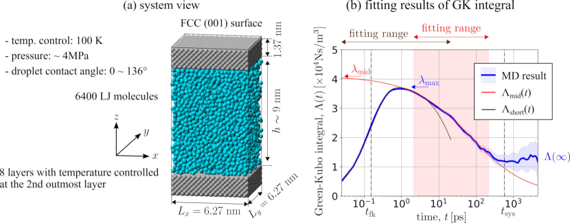
Figure 1: (a) MD simulation system of LJ liquid between flat fcc walls. (b) (Blue) GK integral $\Lambda(t)$ for $\varepsilon^{\mathrm{fs}}=0.310\varepsilon^{\mathrm{ff}}$, and fitting curves for (red) $\Lambda_{\mathrm{mid}}(t)$ with Eq. (19), and (brown) $\Lambda_{\mathrm{short}}(t)$ with Eq. (24). The maximum value $\lambda_{\mathrm{max}}$ as well as $\Lambda(\infty)$ used to compute $\lambda_{\infty}$ are also indicated. Finally, the timescales $t_{\mathrm{fk}}$ and $t_{\mathrm{sys}}$ are represented on the time axis.

Figure 1 (b) illustrates the four EMD calculation methods of the FC from the GK integrals $\Lambda(t)$ listed in Table 1 for a system with $\varepsilon^{\mathrm{fs}}=0.310\varepsilon^{\mathrm{ff}}$. For $\lambda_{\text{mid}}$, we fitted the GK integral with Eq. (19) as the red curved-line in Fig. 1 (b). The set of fitting parameters is $(\lambda_{0},\,t_{\mathrm{slip}})$, and the fitting range is $(t^{\text{fit}}_{\text{mid}},\,10t^{\text{fit}}_{\text{mid}})$, where 10 values for $t^{\text{fit}}_{\text{mid}}$ were tested in the range of 2.14 ps and 21.4 ps at equal log-scale intervals. For $\lambda_{\mathrm{short}}$, we fitted the GK integral $\Lambda(t)$ by

$$\Lambda_{\mathrm{short}}(t)=\lambda_{0}\left(e^{-\frac{t}{t_{1}}}-e^{-\frac{t}{t_{2}}}\right)$$ (24)

as proposed in our previous study [32] as the brown line in Fig. 1 (b), where the set of fitting parameters is $(\lambda_{0},\,t_{1},\,t_{2})$ and the fitting range is $(0,\,t^{\text{fit}}_{\text{short}})$ with 10 different values of $t^{\text{fit}}_{\text{short}}$ tested in the range of 2.14 ps and 21.4 ps at equal log-scale intervals. As observed in Fig. 1 (b), the red and brown fitting lines corresponding to $\Lambda_{\mathrm{mid}}(t)$ in Eq. (19) and $\Lambda_{\mathrm{short}}(t)$ in Eq. (24) reproduce $\Lambda(t)$ well for their fitting ranges, and from these fitting curves, we extract $\lambda_{\mathrm{mid}}$ (displayed with the red arrow) and $\lambda_{\mathrm{short}}$. In addition, we calculated the other two FC approximations $\lambda_{\mathrm{max}}$ and $\lambda_{\infty}$ from the maximum of $\Lambda(t)$ in Eq. (6) and the convergence value $\Lambda(\infty)$ in Eq. (14). For simple cases including this example with $\Lambda(t)$ showing a simple behavior of increasing within a short time and decaying after taking the maximum, the former three give similar results, with slight difference with $\lambda_{\mathrm{mid}},\lambda_{\mathrm{short}}>\lambda_{\mathrm{max}}$; however, we will see later that it is not the case with structured walls. On the other hand, as mentioned in Sec. I, the final plateau value of $\Lambda(t)$ showed large fluctuation as seen in the right-end of the blue curved line Fig. (1), from which $\lambda_{\infty}$ is evaluated including additional calculation of $\eta$ and $h$ obtained in different systems.

To determine the liquid height $h$ used to compute $\lambda_{\infty}$ and $\lambda_{\mathrm{NEMD}}$, we considered that the S-L interface position $z_{\mathrm{SL}}$ was approximately $\sigma^{\mathrm{fs}}$ outward the wall surface for the present case,[25, 42] and we defined $h$ as:

$$h=z_{\mathrm{SL}}^{\mathrm{top}}-z_{\mathrm{SL}}^{\mathrm{bot}}.$$ (25)

The slip velocity $u_{\mathrm{slip}}$ used to evaluate $\lambda_{\mathrm{NEMD}}$ was then given by:

$$u_{\mathrm{slip}}\equiv\frac{1}{2}\left[(u_{\mathrm{w}}^{\mathrm{top}}-u_{\mathrm{w}}^{\mathrm{bot}})-h\left(\frac{\partial u}{\partial z}\right)_{\mathrm{bulk}}\right]=u_{\mathrm{w}}-\frac{h}{2}\left(\frac{\partial u}{\partial z}\right)_{\mathrm{bulk}}$$ (26)

where $\left(\frac{\partial u}{\partial z}\right)_{\mathrm{bulk}}$ was obtained by fitting the average velocity distribution of the liquid bulk with a linear function of $z$.

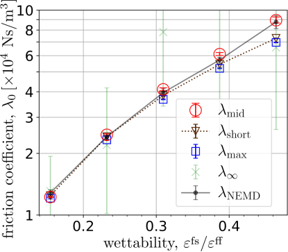
Figure 2: FC for various wettability $\varepsilon^{\mathrm{fs}}$. The calculation methods for each of the 5 estimates of the FC are shown in Table. 1.

Figure 2 shows the FCs obtained for various wettabilities –controlled through $\varepsilon^{\mathrm{fs}}$, where we calculated $\lambda_{\mathrm{mid}}$ and $\lambda_{\mathrm{short}}$ as the average for various fitting ranges. The error bars show the uncertainties due to the fitting range and due to the fluctuation of the GK integral $\Lambda(t)$, which gives larger uncertainty as $t$ increases (the former was much smaller than the latter). Regarding the comparison with the reference NEMD value $\lambda_{\mathrm{NEMD}}$, $\lambda_{\mathrm{mid}}$ –proposed in this study– reproduced $\lambda_{\mathrm{NEMD}}$ the best in comparison with $\lambda_{\mathrm{max}}$ and $\lambda_{\mathrm{short}}$, which overall underestimated $\lambda_{0}$, especially for larger FC on more wetting surfaces. One can also note that the error bars for $\lambda_{\infty}$ were too large to precisely evaluate $\lambda_{0}$, at least with the present calculation cost.

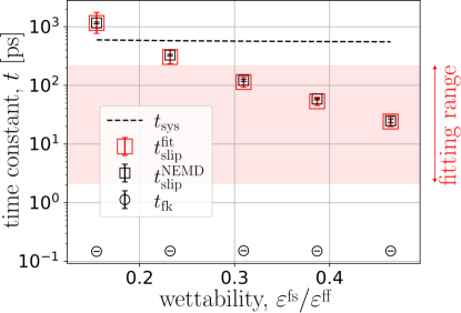
Figure 3: Time scales as a function of wettability; $t_{\mathrm{sys}}=\rho h^{2}/\eta$, $t_{\mathrm{slip}}^{\text{fit}}$ obtained as a fitting parameter of Eq. (19), $t_{\mathrm{slip}}^{\text{NEMD}}=\rho\eta/\lambda_{\mathrm{NEMD}}^{2}$, and $t_{\lambda}$ obtained by fitting $\langle F_{\text{w}}(t)F_{\text{w}}(0)\rangle/Sk_{\mathrm{B}}T$ with the Maxwell-type friction in Eq. (9).

As mentioned in Sec. II, there are three key timescales $t_{\mathrm{fk}}$, $t_{\mathrm{sys}}$, and $t_{\mathrm{slip}}$ for the GK integral $\Lambda(t)$, and for the present fitting by Eq. (19), the timescale $t_{\mathrm{slip}}$ must be basically separated from $t_{\mathrm{fk}}$ and $t_{\mathrm{sys}}$. To check this separation, we estimated the three timescales in the present systems. For $t_{\mathrm{fk}}$, considering that the friction kernel $\lambda(t)$ can be well approximated by the correlation function in the RHS of Eq. (27) on a short timescale as [43]

$$\lambda(t)\approx\frac{1}{Sk_{\mathrm{B}}T}\langle F_{\mathrm{w}}(t)F_{\mathrm{w}}(0)\rangle,$$ (27)

we fitted the RHS of Eq. (27) by the Maxwell-type friction kernel in Eq. (9). We estimated $t_{\mathrm{slip}}$ following two approaches, which we denote by $t_{\mathrm{slip}}^{\mathrm{mid}}$ and $t_{\mathrm{slip}}^{\mathrm{NEMD}}$, respectively: 1) evaluating it as a fitting parameter for $\lambda_{\mathrm{mid}}$ with Eq. (19); and 2) calculating $t_{\mathrm{slip}}$ from the FC $\lambda_{\mathrm{NEMD}}$ obtained by NEMD as

$$t_{\mathrm{slip}}^{\mathrm{NEMD}}\equiv\frac{\rho\eta}{\lambda_{\mathrm{NEMD}}^{2}}.$$ (28)

The density and viscosity values $\rho$ and $\eta$ in Eq. (28) were obtained in the NEMD systems, where $\eta$ was evaluated by

$$\eta\equiv\frac{\tau_{\mathrm{w}}^{\mathrm{NEMD}}}{\left(\frac{\partial u}{\partial z}\right)_{\mathrm{bulk}}},$$ (29)

using the average solid-liquid shear force per area $\tau_{\mathrm{w}}^{\mathrm{NEMD}}$ measured on the solid surface. These values were also used for the evaluation of $t_{\mathrm{sys}}$ given by Eq. (20). Since the present systems were under pressure and temperature control, the resulting $\rho$ and $\eta$ were constant. On the other hand, $h$ slightly depended on the wettability $\varepsilon^{\mathrm{fs}}$ under this condition with a constant number of fluid particles, hence, $t_{\mathrm{sys}}$ slightly depended on the wettability, too.

Figure 3 shows the comparison among the three timescales. For the present system, $t_{\mathrm{slip}}$ depended largely on the wettability $\varepsilon^{\mathrm{fs}}$ as easily imagined from Eq. (18) with the results of $\lambda_{\mathrm{mid}}$ in Fig. 2. This was in contrast to $t_{\mathrm{fk}}$, which was overall below one picosecond and was almost independent of the wettability. In addition, the system timescale $t_{\mathrm{sys}}$ was about several hundreds of picoseconds. Hence, the timescale separation in Ineq. (21) was well satisfied for $\varepsilon^{\mathrm{fs}}\geq 0.3\varepsilon^{\mathrm{ff}}$; however, even for the case of $\varepsilon^{\mathrm{fs}}=0.1\varepsilon^{\mathrm{ff}}$ where $t_{\mathrm{slip}}$ was larger than $t_{\mathrm{sys}}$, the present result $\lambda_{\mathrm{mid}}$ still gave a good estimate of $\lambda_{\mathrm{NEMD}}$. This is probably because of the features of the hyperbolic functions $\sinh$ and $\cosh$ in Eq. (10), which quickly approach to the limit for $h\rightarrow\infty$ in Eq. (16).

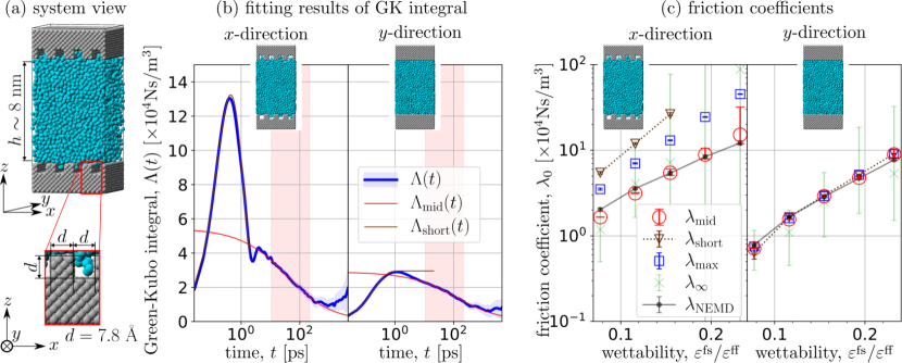
Figure 4: (a) System view with grooved walls for $\varepsilon^{\mathrm{fs}}=0.155\varepsilon^{\mathrm{ff}}$. (b) GK integrals $\Lambda(t)$ in the (left) $x$- and (right) $y$-directions and their fitting curves; Blue: GK integral, red: fitting curve for $\lambda_{\mathrm{mid}}$, and brown: fitting curve for $\lambda_{\mathrm{short}}$. (c) Obtained FCs for various wettability $\varepsilon^{\mathrm{fs}}$ in the (left) $x$- and (right) $y$-directions; the calculation methods are summarized in Table 1.

In addition to the analysis on flat surfaces shown above, we applied the FC measurement methods to the S-L friction on grooved surfaces as exemplified in Fig. 4(a). For each $\varepsilon^{\mathrm{fs}}$, two NEMD simulations with shearing in the $x$- and $y$-directions were carried out to obtain $\lambda_{\mathrm{NEMD}}$ considering the heterogeneous structure of the surface. In the following, we will denote $u$ and $v$ the velocity along the $x$- and $y$-directions, respectively. Since the density and momentum are inhomogeneous in the $xy$-plane near the wall surface, there is no clear definition of the slip velocity or the interface position. Here we defined the slip velocity $u_{\mathrm{slip}}$ or $v_{\mathrm{slip}}$ for the NEMD based on Eqs. (25) and (26) as follows. First, the distributions of mass and momentum density in the $x$- or $y$-direction were calculated as the average over the $xy$-plane. Second, the velocity distribution obtained as momentum density per mass density was fitted only in the bulk part with a linear function to obtain $\left(\frac{\partial u}{\partial z}\right)_{\mathrm{bulk}}$ in Eq. (26) or $\left(\frac{\partial v}{\partial z}\right)_{\mathrm{bulk}}$ as in the flat wall systems, and finally the slip velocity was obtained by extrapolating the fitted velocity distribution to the positions $z_{\mathrm{SL}}^{\mathrm{top}}$ and $z_{\mathrm{SL}}^{\mathrm{bot}}$ in Eq. (25) at $\sigma_{\text{fs}}$ from the top of the grooved wall surface toward the liquid bulk. An EMD simulation was also run for each $\varepsilon^{\mathrm{fs}}$ to obtain $\Lambda^{x}(t)$ and $\Lambda^{y}(t)$ in the two directions using $F_{\mathrm{w}}^{x}$ and $F_{\mathrm{w}}^{y}$ as the S-L friction force $F_{\mathrm{w}}$ in Eq. (5).

Figure 4(b) shows an example of the GK integrals $\Lambda^{x}(t)$ and $\Lambda^{y}(t)$ for the grooved surface system, with $\varepsilon^{\mathrm{fs}}=0.155\varepsilon^{\mathrm{ff}}$. The GK integrals $\Lambda^{x}(t)$ in the left panel have a complex shape, with a sharp peak in the short timescale below a few picoseconds, and a slow decay afterwards, which was not observed for $\Lambda^{y}(t)$ in the right panel nor $\Lambda(t)$ for the flat wall system in Fig. 1(b). This short-time behavior is due to the local vibration of the fluid particles confined in the grooves, and not related to the hydrodynamic motion. We fitted $\Lambda_{\mathrm{short}}(t)$ and $\Lambda_{\mathrm{mid}}(t)$ to $\Lambda^{x}(t)$ and $\Lambda^{y}(t)$ shown with brown and red lines to obtain $\lambda_{\mathrm{short}}$ and $\lambda_{\mathrm{mid}}$ in both directions as well as $\lambda_{\mathrm{max}}$ summarized in Table 1. Figure 4(c) shows the comparison between the estimated $\lambda_{0}$ in the $x$- and $y$-directions. As imagined from the complex GK-integral $\Lambda^{x}(t)$, $\lambda_{\mathrm{short}}$ and $\lambda_{\mathrm{max}}$ in the $x$-direction (left panel) using the short timescale resulted in much larger estimate than $\lambda_{\mathrm{mid}}$, while the latter corresponded well with the NEMD estimate $\lambda_{\mathrm{NEMD}}$. On the other hand, for the FC in the $y$-direction (left panel), all EMD estimates except $\lambda_{\infty}$ reproduced $\lambda_{\mathrm{NEMD}}$ well. This also indicates that the present NEMD estimate using the above-mentioned definition of the slip velocity was reasonable. Considering the two results, the present FC measurement method $\lambda_{\mathrm{mid}}$ properly evaluates the FC even in this heterogeneous-wall system.

V CONCLUDING REMARKS

In this study, we proposed a method to calculate the solid-liquid FC from EMD simulations of a liquid confined between parallel solid walls, by fitting the GK integral for the timescale range where the GK integral slowly decays with time. The fitting function was derived from the analytical solution considering that the timescales of the friction kernel and bulk viscous dissipation can be separated. We compared the resulting FCs with those obtained with other EMD-based methods and with NEMD simulations, for a Lennard-Jones liquid confined between flat crystalline walls as well as between grooved walls with different wettability, and showed that the present method extracts the FC with excellent accuracy for various systems, with easy implementation and low calculation cost.

DATA AVAILABILITY

The data that support the findings of this study are available from the corresponding author upon reasonable request.

AUTHOR DECLARATIONS
Conflict of Interest

The authors have no conflicts to disclose.

Appendix A Derivation of a theoretical solution of the GK integral

A.1 Derivation through the combination of Langevin equation and Stokes equation

We consider a system where a liquid is confined between two solid walls under no external field, where the top wall is fixed. Let the bottom wall move freely in a wall-tangential direction $x$; its motion can be described by a generalized Langevin equation:[29]

$$M\frac{\mathrm{d}\,U}{\mathrm{d}\,t}=-S\int_{0}^{t}\xi(t-t^{\prime})U(t^{\prime})\,\mathrm{d}t^{\prime}+F_{\mathrm{w}}(t),$$ (30)

where $M$, $S$ and $U$ are the mass, the surface area and the $x$-direction velocity of the bottom wall respectively; $\xi$ is the friction kernel and $F_{\mathrm{w}}$ is the random force that originates from the direct interaction between the solid and liquid particles. Assuming energy equipartition, Eq. (30) leads to the fluctuation-dissipation theorem:

$$C_{F_{\mathrm{w}}}(t)\equiv\left<F_{\mathrm{w}}(t)\,F_{\mathrm{w}}(0)\right>=Sk_{\mathrm{B}}T\xi(t).$$ (31)

The motion of the liquid in response to the bottom wall motion can be described by the Stokes equation:

$$\frac{\partial u(z,t)}{\partial t}=\frac{\eta}{\rho}\frac{\partial^{2}u(z,t)}{\partial{z}^{2}}$$ (32)

with the Navier boundary condition defined on the top and bottom hydrodynamic boundaries at $z=0$ and $h$ respectively given by

$$\begin{cases}\eta\left.\frac{\partial u(z,t)}{\partial z}\right|_{z=h}=\int_{0}^{t}\lambda(t-t^{\prime})\left[-u(h,t^{\prime})\right]\,\mathrm{d}t^{\prime},\\[5.69054pt] \eta\left.\frac{\partial u(z,t)}{\partial z}\right|_{z=0}=\int_{0}^{t}\lambda(t-t^{\prime})\left[u(0,t^{\prime})-U(t^{\prime})\right]\,\mathrm{d}t^{\prime},\end{cases}$$ (33)

where $u$, $t$, $\rho$, $\eta$ and $\lambda$ denote the liquid velocity in the $x$-direction, the time, the bulk liquid density, the bulk liquid viscosity, and the Navier friction coefficient (FC), respectively. Note that the non-Markovian nature is included in $\lambda$.[42] Denoting the Fourier-Laplace transformed variables with tilde as

$$\tilde{f}(\omega)\equiv\int_{0}^{\infty}f(t)e^{-i\omega t}\text{d}t,$$

the solution of Eqs. (32) and (33) is written in a compact form as $\tilde{u}=\tilde{\gamma}\tilde{U}$ for the liquid velocity on the bottom wall with

$$\tilde{\gamma}=\frac{\tilde{\lambda}\left[\tilde{\lambda}\sinh(\zeta h)+\eta\zeta\cosh(\zeta h)\right]}{(\tilde{\lambda}^{2}+\eta^{2}\zeta^{2})\sinh(\zeta h)+2\tilde{\lambda}\eta\zeta\cosh(\zeta h)}.$$ (34)

Because the first term on the right hand side of Eq. (30) can also be rewritten as

$$-S\int_{0}^{t}\xi(t-t^{\prime})U(t^{\prime})\,\mathrm{d}t^{\prime}=-S\int_{0}^{t}\lambda(t-t^{\prime})[U(t^{\prime})-u(0,t^{\prime})]\,\mathrm{d}t^{\prime}$$ (35)

in terms of the slip velocity on the wall, the friction kernel $\xi$ can be written as

$$\tilde{\xi}=\tilde{\lambda}(1-\tilde{\gamma}).$$ (36)

Combined with Eq. (31), the expression for the force autocorrelation function writes

$$\frac{\tilde{C}_{F_{\mathrm{w}}}}{Sk_{B}T}=\frac{\tilde{\lambda}\eta\zeta\left[\eta\zeta\sinh(\zeta h)+\tilde{\lambda}\cosh(\zeta h)\right]}{(\tilde{\lambda}^{2}+\eta^{2}\zeta^{2})\sinh(\zeta h)+2\tilde{\lambda}\eta\zeta\cosh(\zeta h)},$$

where $\zeta$ is given by

$$\zeta=\sqrt{\frac{i\rho\omega}{\eta}}$$

as a function of the angular frequency $\omega$.

A.2 Asymptotic behavior

As one of possible methods to obtain $\lambda_{0}$, we proposed to use the convergence value $\Lambda(\infty)$ in our previous study,[43] in which we used the following relations:

$$\lim_{\omega\rightarrow 0}\frac{\tilde{C}_{F_{\mathrm{w}}}(\omega)}{Sk_{\mathrm{B}}T}=\lim_{\omega\rightarrow 0}\int_{0}^{\infty}\frac{C_{F_{\mathrm{w}}}(t)}{Sk_{\mathrm{B}}T}e^{-i\omega t}dt=\lim_{t\rightarrow\infty}\Lambda(t),$$ (37)

and

$$\lim_{\omega\rightarrow 0}\tilde{\lambda}(\omega)=\lim_{\omega\rightarrow 0}\int_{0}^{\infty}\lambda(t)e^{-i\omega t}dt=\lambda_{0}.$$ (38)

By inserting Eqs. (A.1) and (A.1) into Eq. (37), it follows for the convergence value of the GK integral that

$$\lim_{t\rightarrow\infty}\Lambda(t) =\lim_{\omega\rightarrow 0}\frac{\tilde{\lambda}\eta\zeta\left[\eta\zeta\sinh(\zeta h)+\tilde{\lambda}\cosh(\zeta h)\right]}{(\tilde{\lambda}^{2}+\eta^{2}\zeta^{2})\sinh(\zeta h)+2\tilde{\lambda}\eta\zeta\cosh(\zeta h)}$$

$$=\lim_{\omega\rightarrow 0}\frac{\eta\zeta\tanh(\zeta h)+\tilde{\lambda}}{\left(\frac{\tilde{\lambda}}{\eta\zeta}+\frac{\eta\zeta}{\tilde{\lambda}}\right)\tanh(\zeta h)+2}.$$ (39)

By considering Eq. (12) and

$$\lim_{\zeta h\rightarrow 0}\frac{\tanh(\zeta h)}{\zeta h}=1,$$ (40)

Eq. (A.2) results in

$$\lim_{t\rightarrow\infty}\Lambda(t) =\lim_{\omega\rightarrow 0}\frac{\eta\zeta\cdot\zeta h\frac{\tanh(\zeta h)}{\zeta h}+\tilde{\lambda}}{\left(\frac{\tilde{\lambda}}{\eta\zeta}+\frac{\eta\zeta}{\tilde{\lambda}}\right)\zeta h\frac{\tanh(\zeta h)}{\zeta h}+2}$$

$$=\frac{\lambda_{0}}{\frac{h}{\eta}\lambda_{0}+2}=\frac{\lambda_{0}}{\frac{h}{b}+2},$$ (13)

where Eq. (4) is used for the final equality. Hence, from Eqs. (4) and (A.2) $\lambda_{0}$ can be evaluated by

$$\lambda_{0}=\frac{2\Lambda(\infty)}{1-\frac{h}{\eta}\Lambda(\infty)}.$$ (41)

Appendix B velocity distribution of Couette flow system

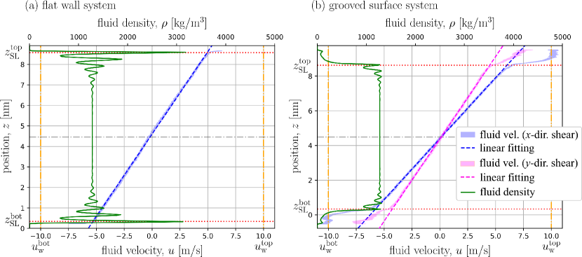
Figure 5: Distributions of the fluid velocity and density for (a) flat wall system with $\varepsilon^{\mathrm{fs}}=0.310\varepsilon^{\mathrm{ff}}$, and (b) grooved surface system with $\varepsilon^{\mathrm{fs}}=0.155\varepsilon^{\mathrm{ff}}$. Blue: (solid) fluid velocity distribution for $x$-direction shear and (dashed) linear fitting. Magenta: (solid) fluid velocity distribution for $y$-direction shear and (dashed) linear fitting. Green: fluid density. Red dotted lines: positions of the top and bottom solid-liquid interfaces $z^{\mathrm{top}}_{\mathrm{SL}}$ and $z^{\mathrm{bot}}_{\mathrm{SL}}$. Orange dashed lines: wall velocities $u_{\mathrm{w}}^{\mathrm{bot}}$ and $u_{\mathrm{w}}^{\mathrm{top}}$.

Non-equilibrium MD (NEMD) simulations of Couette-type flow were performed to compute the friction coefficient (FC) $\lambda_{\mathrm{NEMD}}$. Figure  5 shows examples of the distributions of the fluid velocity and density, where two Couette-type MD simulations with shear in the $x$- and $y$-directions were carried out for each wettability parameter $\varepsilon^{\mathrm{fs}}$ by moving the top and bottom walls in opposite directions ($\pm x$- or $\pm y$-directions), whilst single simulation ($x$-shear) was run for a flat wall system considering the symmetry of the system. The velocity distributions with shear in the $x$- and $y$-directions for the grooved surface systems are shown in blue and pink, respectively in Fig. 5(b). Indeed, the velocity and density distributions were not completely quasi-one-dimensional, and the streamline was not parallel to the shear direction for the grooved surface system especially around the wall, e.g., the velocities at two points above the concave and convex regions with the same $z$-coordinate were different, but the velocity inhomogeniety in the $xy$-plane quickly vanished and the time-averaged velocity distribution away from the wall was considered to be quasi-one-dimensional. Considering that the present framework is based on the one-dimension Stokes equation as described in Appendix A, we averaged the physical quantities in the $xy$-plane to extract $\lambda_{\mathrm{NEMD}}$ in this study. The positions of the top and bottom solid-liquid interfaces $z^{\mathrm{top}}_{\mathrm{SL}}$ and $z^{\mathrm{bot}}_{\mathrm{SL}}$ are indicated by the red lines in the Fig. 5 (see the definition in the main text). In the case of Fig. 5(b), the slip velocity for the shear in the $x$-direction is smaller than that for the shear in the $y$-direction.

Appendix C friction kernel

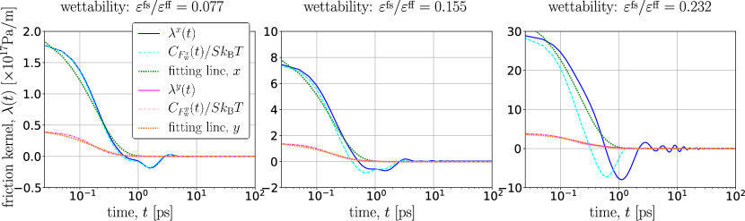
Figure 6: Friction kernel $\lambda(t)$ for grooved surface systems with wettability parameter $\varepsilon^{\mathrm{fs}}$ of (left) $0.077\varepsilon^{\mathrm{ff}}$, (center) $0.155\varepsilon^{\mathrm{ff}}$, and (right) $0.232\varepsilon^{\mathrm{ff}}$. Blue: (solid) friction kernel $\lambda(t)$ and (dashed) $C_{F_{\mathrm{w}}}(t)/Sk_{\mathrm{B}}T$ for the $x$-direction. Magenta (solid) friction kernel $\lambda(t)$ and (dashed) $C_{F_{\mathrm{w}}}(t)/Sk_{\mathrm{B}}T$ for the $y$-direction. Fitting lines with the Maxwell-type kernel in Eq. (9) are shown in green and orange as well.

To investigate the complex shape of GK integral $\Lambda^{x}(t)$ in Fig. 4, we numerically solved Eq. (10) with respect to $\lambda(t)$ for the grooved surface system using the method proposed in our previous study;[43] at first, we calculated $\tilde{\lambda}(\omega)$ by numerically solving Eq. (10) by using the FL-transform $\tilde{C}_{F_{\mathrm{w}}}(\omega)$ of the autocorrelation function ${C}_{F_{\mathrm{w}}}(t)$, and then, we obtained $\lambda(t)$ by performing the inverse-FL transform of $\tilde{\lambda}(\omega)$. Figure 6 shows the results of $\lambda(t)$ obtained for (blue) $x$- and (magenta) $y$-directions. The friction kernel $\lambda(t)$ corresponded well with $\frac{C_{F_{\mathrm{w}}}(t)}{Sk_{\mathrm{B}}T}$ shown in cyan and pink in the $x$- and $y$-directions, respectively for small friction coefficients, i.e., for low wettability. This is consistent with the fact that Eq. (27) holds when

$$\sqrt{\frac{\eta t}{\rho}}\ll\min\left(\left|\frac{\eta}{\tilde{\lambda}}\right|,h\right)$$ (42)

is satisfied.[43] We also attempted to fit the kernel by the Maxwell type kernel in Eq. (9) as shown with green and orange lines. The kernel $\lambda(t)$ can be well approximated by the Maxwell type kernel for the $y$-direction, whilst the complex kernel shape cannot be properly expressed by the Maxwell type kernel for the $x$-direction. The oscillating behavior of the friction kernel $\lambda(t)$ observed for $\varepsilon^{\mathrm{fs}}=0.232\varepsilon^{\mathrm{ff}}$ in the $x$-direction within a short timescale $<10$ ps is supposed to be due to the vibration of the fluid particles confined in the groove. Indeed, this complex kernel shape $\lambda^{x}(t)$ is reflected in the complex GK integral $\Lambda^{x}(t)$ in Fig. 4.

References

- Eijkel and van den Berg [2005] J. C. Eijkel and A. van den Berg, Microfluid. Nanofluidics 1, 249 (2005).
- Sparreboom et al. [2009] W. Sparreboom, A. van den Berg, and J. C. Eijkel, Nat. Nanotechnol. 4, 713 (2009).
- Bocquet and Charlaix [2010] L. Bocquet and E. Charlaix, Chem. Soc. Rev. 39, 1073 (2010).
- Schoch et al. [2008] R. B. Schoch, J. Han, and P. Renaud, Rev. Mod. Phys. 80, 839 (2008).
- Sparreboom et al. [2010] W. Sparreboom, A. van den Berg, and J. C. Eijkel, New J. Phys. 12, 015004 (2010).
- Striolo et al. [2016] A. Striolo, A. Michaelides, and L. Joly, Annu. Rev. Chem. Biomol. Eng. 7, 533 (2016).
- Navier [1823] C. Navier, Mémoires de l’Académie Royale des Sciences de l’Institut de France 6, 389 (1823).
- Falk et al. [2010] K. Falk, F. Sedlmeier, L. Joly, R. R. Netz, and L. Bocquet, Nano Lett. 10, 4067 (2010).
- Keerthi et al. [2021] A. Keerthi, S. Goutham, Y. You, P. Iamprasertkun, R. A. Dryfe, A. K. Geim, and B. Radha, Nat. Commun. 12, 3092 (2021).
- Chen et al. [2021] K.-T. Chen, Q.-Y. Li, T. Omori, Y. Yamaguchi, T. Ikuta, and K. Takahashi, Carbon 189, 162 (2021).
- Huang et al. [2008] D. M. Huang, C. Cottin-Bizonne, C. Ybert, and L. Bocquet, Langmuir 24, 1442 (2008).
- Ogawa et al. [2019] K. Ogawa, H. Oga, H. Kusudo, Y. Yamaguchi, T. Omori, S. Merabia, and L. Joly, Phys. Rev. E 100, 023101 (2019).
- Thompson and Robbins [1990] P. A. Thompson and M. O. Robbins, Phys. Rev. A 41, 6830 (1990).
- Thompson and Troian [1997] P. A. Thompson and S. M. Troian, Nature 389, 360 (1997).
- Barrat and Bocquet [1999] J. L. Barrat and L. Bocquet, Faraday Discuss. 112, 119 (1999).
- Cieplak et al. [2001] M. Cieplak, J. Koplik, and J. R. Banavar, Phys. Rev. Lett. 86, 803 (2001).
- Kannam et al. [2013] S. K. Kannam, B. D. Todd, J. S. Hansen, and P. J. Daivis, J. Chem. Phys. 138, 094701 (2013).
- Bhatia and Nicholson [2013] S. K. Bhatia and D. Nicholson, Langmuir 29, 14519 (2013).
- Tocci et al. [2014] G. Tocci, L. Joly, and A. Michaelides, Nano Lett. 14, 6872 (2014).
- Guo et al. [2016] L. Guo, S. Chen, and M. O. Robbins, Eur. Phys. J. Spec. Top. 225, 1551 (2016).
- Nakaoka et al. [2017a] S. Nakaoka, Y. Yamaguchi, T. Omori, and L. Joly, J. Chem. Phys. 146, 174702 (2017a).
- Ewen et al. [2019] J. P. Ewen, H. Gao, M. H. Müser, and D. Dini, Phys. Chem. Chem. Phys. 21, 5813 (2019).
- Kannam et al. [2011] S. K. Kannam, B. D. Todd, J. S. Hansen, and P. J. Daivis, J. Chem. Phys. 135, 144701 (2011).
- Kumar Kannam et al. [2012] S. Kumar Kannam, B. D. Todd, J. S. Hansen, and P. J. Daivis, J. Chem. Phys. 136, 024705 (2012).
- Herrero et al. [2019] C. Herrero, T. Omori, Y. Yamaguchi, and L. Joly, J. Chem. Phys. 151, 041103 (2019).
- Bocquet and Barrat [1994] L. Bocquet and J. L. Barrat, Phys. Rev. E 49, 3079 (1994).
- Petravic and Harrowell [2007] J. Petravic and P. Harrowell, J. Chem. Phys. 127, 174706 (2007).
- Hansen et al. [2011] J. S. Hansen, B. D. Todd, and P. J. Daivis, Phys. Rev. E 84, 016313 (2011).
- Bocquet and Barrat [2013] L. Bocquet and J. L. Barrat, J. Chem. Phys. 139, 044704 (2013).
- Huang and Szlufarska [2014] K. Huang and I. Szlufarska, Phys. Rev. E 89, 032119 (2014).
- Sam et al. [2018] A. Sam, R. Hartkamp, S. K. Kannam, and S. P. Sathian, Nanotechnology 29, 485404 (2018).
- Oga et al. [2019] H. Oga, Y. Yamaguchi, T. Omori, S. Merabia, and L. Joly, J. Chem. Phys. 151, 054502 (2019).
- Varghese et al. [2021] S. Varghese, J. S. Hansen, and B. D. Todd, J. Chem. Phys. 154, 184707 (2021).
- Nakano and Sasa [2020] H. Nakano and S. Sasa, Phys. Rev. E 101, 033109 (2020).
- Sokhan and Quirke [2008] V. P. Sokhan and N. Quirke, Phys. Rev. E 78, 015301(R) (2008).
- Hadjiconstantinou and Swisher [2022] N. G. Hadjiconstantinou and M. M. Swisher, Phys. Rev. Fluids 7, 114203 (2022).
- Evans and Morriss [2008] D. Evans and G. Morriss, Statistical Mechanics of Nonequilibrium Liquids, 2nd ed. (Cambridge University Press, 2008) pp. 71–72.
- Español et al. [2019] P. Español, J. A. De La Torre, and D. Duque-Zumajo, Phys. Rev. E 99, 022126 (2019).
- Merabia and Termentzidis [2012] S. Merabia and K. Termentzidis, Phys. Rev. B 86, 094303 (2012).
- Nakaoka et al. [2017b] S. Nakaoka, Y. Yamaguchi, T. Omori, and L. Joly, Mech. Eng. Lett. 3, 17 (2017b).
- Schulz et al. [2020] J. C. F. Schulz, A. Schlaich, M. Heyden, R. R. Netz, and J. Kappler, Phys. Rev. Fluids 5, 103301 (2020).
- Omori et al. [2019] T. Omori, N. Inoue, L. Joly, S. Merabia, and Y. Yamaguchi, Phys. Rev. Fluids 4, 114201 (2019).
- Oga et al. [2021] H. Oga, T. Omori, C. Herrero, S. Merabia, L. Joly, and Y. Yamaguchi, Phys. Rev. Res. 3, L032019 (2021).
- Nakano and Sasa [2019a] H. Nakano and S. Sasa, J. Stat. Phys. 176, 312 (2019a).
- Nakano and Sasa [2019b] H. Nakano and S. Sasa, Phys. Rev. E 99, 013106 (2019b).
- Thompson et al. [2022] A. P. Thompson, H. M. Aktulga, R. Berger, D. S. Bolintineanu, W. M. Brown, P. S. Crozier, P. J. in’t Veld, A. Kohlmeyer, S. G. Moore, T. D. Nguyen, R. Shan, M. J. Stevens, J. Tranchida, C. Trott, and S. J. Plimpton, Comput. Phys. Commun. 271, 108171 (2022).
- Nishida et al. [2014] S. Nishida, D. Surblys, Y. Yamaguchi, K. Kuroda, M. Kagawa, T. Nakajima, and H. Fujimura, J. Chem. Phys. 140, 074707 (2014).
- Nakaoka et al. [2015] S. Nakaoka, Y. Yamaguchi, T. Omori, M. Kagawa, T. Nakajima, and H. Fujimura, Phys. Rev. E 92, 022402 (2015).